Hexagonalization of Correlation Functions II :
Two-Particle Contributions

Thiago Fleury, Shota Komatsu

Instituto de Física Teórica, UNESP - Univ. Estadual Paulista, ICTP South American Institute for Fundamental Research, Rua Dr. Bento Teobaldo Ferraz 271, 01140-070, São Paulo, SP, Brasil
Laboratoire de Physique Théorique de l’Ecole Normale Supérieure et l’Université Paris-VI, 24 rue Lhomond, Paris CEDEX 75231, France
International Institute of Physics, Federal University of Rio Grande do Norte,
Campus Universitário, Lagoa Nova, Natal, RN 59078-970, Brazil
School of Natural Sciences, Institute for Advanced Study, Princeton, NJ 08540, USA

Abstract

In this work, we compute one-loop planar five-point functions in 𝒩𝒩\mathcal{N}=4 super-Yang-Mills using integrability. As in the previous work, we decompose the correlation functions into hexagon form factors and glue them using the weight factors which depend on the cross-ratios. The main new ingredient in the computation, as compared to the four-point functions studied in the previous paper, is the two-particle mirror contribution. We develop techniques to evaluate it and find agreement with the perturbative results in all the cases we analyzed. In addition, we consider next-to-extremal four-point functions, which are known to be protected, and show that the sum of one-particle and two-particle contributions at one loop adds up to zero as expected. The tools developed in this work would be useful for computing higher-particle contributions which would be relevant for more complicated quantities such as higher-loop corrections and non-planar correlators.

1 Introduction

The planar 𝒩𝒩\mathcal{N}=4 super-Yang-Mills is believed to be an integrable theory [1] to all orders in perturbation theory111For more recent progress, in particular about the quantum spectral curve method, see the original article [2] and also the lecture notes [3].. Recently, an integrability-based method for computing the four- [4, 5] and higher-point [5] correlation functions, named hexagonalization, was proposed. The method consists in cutting the correlation functions into smaller building blocks called the hexagon form factors which were first introduced in [6] in the context of the three-point functions. To be more concrete, take for example a planar n𝑛n-point function. Pictorially, it can be represented as a sphere with n𝑛n holes and one cuts this surface into 2(n2)2𝑛22(n-2) hexagonal patches. The contribution from each patch is given by the hexagon form factor, and by gluing these hexagons with appropriate weight factor, one can compute the original correlation function222Alternatively, one could perform the OPE and then compute the structure constants using the integrability [7]. However this OPE method involves the mixing with multi-trace operators and it is not clear how to study this mixing systematically. An advantage of using the hexagonalization is that it avoids the mixing problem. It would be very interesting to understand the relation between the two approaches. .

In [5], we applied this method to compute four-point functions at one loop. In this work, we generalize this analysis to some of the one-loop five-point functions. For the sake of simplicity, we consider a restricted kinematics in which all five operators live on a two-dimensional plane333We also impose analogous constraints on the R𝑅R-charge polarizations.. From the computational point of view, the main difference from the previous work is that we now need the two-particle mirror contributions while, in all the calculations done in [5], only the one-particle contribution was needed. We compare our results with the perturbative data [8] and show that they agree. We also show that the integrability result is independent of the way of cutting the worldsheet into hexagons. This property was named the flip invariance in [5]. The way the flip invariance is realized in the five-point functions is much more nontrivial as compared to that for the four-point functions, and it serves as a stringent consistency check of our computation.

The tools developed in this paper should also be useful for computing higher-particles contributions, which would be relevant for higher-point functions and nonplanar correction [9, 10]444It is also interesting to study the non-planar correction to the non-BPS two-point functions. The initial attempt in this direction was made in [11]. The computation is however generally more involved and our tools do not immediately apply to such cases since one also needs to include physical magnons.. As another application of our result, we provide supporting evidence for the prescription conjectured in [5], which states that one only needs to consider the mirror corrections coming from 1-edge irreducible (1EI) graphs, i.e. graphs that are still connected when any bridge with non-zero length is cut. Specifically, we consider one-loop next-to-extremal four-point functions, which consist only of non-1EI graphs, and show that the mirror particle corrections for such correlators cancel among themselves. This is in accordance with the non-renormalization property of the next-to-extremal correlators discussed in [12, 14, 13].

The paper is organized as follows. In section 2, we present the prediction from integrability and compare it with the one-loop perturbative data for five-point functions. In all the examples that we studied, we find a perfect match. We then sketch the strategy of the computation of two-particle contributions in section 3 relegating more technical details to the appendices. The flip invariance is also discussed in great detail in section 3. Using the two-particle contribution, we furthermore show the cancellation of the mirror-particle corrections coming from non-1EI graphs for a near extremal four-point function in section 4. Section 5 has our conclusions. Appendices are basically for explaining the technical details of the computation: Appendix A has the Z𝑍Z-marker prescription which we used to dress the mirror bound state basis. The mirror bound state S𝑆S-matrix is computed in appendix B. The necessary weak coupling expansions are shown in appendix C. The complete two-particle integrand is given in appendix D. There, we also comment on how to evaluate the integral and the prescription to avoid singularities.

2 Five-Point Functions: Perturbation and Integrability

In this section, we compare the integrability result and the perturbative data for five-point functions at one loop. Unlike the four-point functions where a simple closed-form expression is known for BPS operators of any length, such an expression is not known for the five-point functions555In principle, one can use the method of [8] to compute any desired five-point functions. However, a closed-form expression similar to the ones given in [15] is not known.. We are thus going to focus on two examples, the case of five length-two operators and the case of three length-two and two length-three operators, which were computed and written down explicitly in [8]. Another reason why we focus on these two examples is because they receive corrections only from the one- and the two-particle contributions. On the other hand, many other examples such as the correlator of four length-two and one length-four operators needs higher-particle contributions. Although we do not perform the computation of such contributions in this paper, in principle they can be calculated using the tools developed in this paper.

2.1 Set-up

We consider BPS operators and we denote them as

𝒪Li(xi,Yi)=Tr((YiΦ)Li(xi)),subscript𝒪subscript𝐿𝑖subscript𝑥𝑖subscript𝑌𝑖Trsuperscriptsubscript𝑌𝑖Φsubscript𝐿𝑖subscript𝑥𝑖\mathcal{O}_{L_{i}}(x_{i},Y_{i})={\rm{Tr}}\,((Y_{i}\cdot\Phi)^{L_{i}}(x_{i}))\,, (1)

where YiΦ=I=16YiIΦIsubscript𝑌𝑖Φsuperscriptsubscript𝐼16superscriptsubscript𝑌𝑖𝐼superscriptΦ𝐼Y_{i}\cdot\Phi=\sum_{I=1}^{6}Y_{i}^{I}\Phi^{I}. Yisubscript𝑌𝑖Y_{i}’s are null polarization vectors YiYi=0subscript𝑌𝑖subscript𝑌𝑖0Y_{i}\cdot Y_{i}=0, ΦIsuperscriptΦ𝐼\Phi^{I}’s are the six scalars and Lisubscript𝐿𝑖L_{i} is the length of the operator. We normalize the two-point functions of these operators as

𝒪L(x1,Y1)𝒪L(x2,Y2)=(d12)L,delimited-⟨⟩subscript𝒪𝐿subscript𝑥1subscript𝑌1subscript𝒪𝐿subscript𝑥2subscript𝑌2superscriptsubscript𝑑12𝐿\langle\mathcal{O}_{L}(x_{1},Y_{1})\mathcal{O}_{L}(x_{2},Y_{2})\rangle=(d_{12})^{L}\,, (2)

with

dij=yij2xij2,andyij2=YiYj.formulae-sequencesubscript𝑑𝑖𝑗subscriptsuperscript𝑦2𝑖𝑗superscriptsubscript𝑥𝑖𝑗2andsuperscriptsubscript𝑦𝑖𝑗2subscript𝑌𝑖subscript𝑌𝑗d_{ij}=\frac{y^{2}_{ij}}{x_{ij}^{2}}\,,\quad{\rm{and}}\quad y_{ij}^{2}=Y_{i}\cdot Y_{j}\,. (3)

In our normalization, the planar five-point functions of such BPS operators are of the form,

𝒪L1(x1,Y1)𝒪L2(x2,Y2)𝒪L3(x3,Y3)𝒪L4(x4,Y4)𝒪L5(x5,Y5)=delimited-⟨⟩subscript𝒪subscript𝐿1subscript𝑥1subscript𝑌1subscript𝒪subscript𝐿2subscript𝑥2subscript𝑌2subscript𝒪subscript𝐿3subscript𝑥3subscript𝑌3subscript𝒪subscript𝐿4subscript𝑥4subscript𝑌4subscript𝒪subscript𝐿5subscript𝑥5subscript𝑌5absent\displaystyle\langle\mathcal{O}_{L_{1}}(x_{1},Y_{1})\mathcal{O}_{L_{2}}(x_{2},Y_{2})\mathcal{O}_{L_{3}}(x_{3},Y_{3})\mathcal{O}_{L_{4}}(x_{4},Y_{4})\mathcal{O}_{L_{5}}(x_{5},Y_{5})\rangle=
(disconnected)+i=15LiN3G{Li},disconnectedsuperscriptsubscriptproduct𝑖15subscript𝐿𝑖superscript𝑁3subscript𝐺subscript𝐿𝑖\displaystyle\;({\rm{disconnected}})+\frac{\prod_{i=1}^{5}\sqrt{L_{i}}}{N^{3}}\,G_{\{L_{i}\}}\,,

where the first term on the right hand side denotes the disconnected part of the correlator which is given by a product of lower-point functions. In this work, we are only interested in the connected correlator G{Li}subscript𝐺subscript𝐿𝑖G_{\{L_{i}\}} up to one-loop order.

For the sake of simplicity, we are going to work with a restricted kinematics, i.e. we consider the configurations in which the five operators live in a plane both in spacetime and in R𝑅R-charge. This reduces the number of cross ratios from ten (five for spacetime and five for R𝑅R-charge) to eight (four for spacetime and four for R𝑅R-charge). They are defined as

zz¯=x122x342x132x242,(1z)(1z¯)=x142x232x132x242,αα¯=y122y342y132y242,(1α)(1α¯)=y142y232y132y242,formulae-sequence𝑧¯𝑧superscriptsubscript𝑥122superscriptsubscript𝑥342superscriptsubscript𝑥132superscriptsubscript𝑥242formulae-sequence1𝑧1¯𝑧superscriptsubscript𝑥142superscriptsubscript𝑥232superscriptsubscript𝑥132superscriptsubscript𝑥242formulae-sequence𝛼¯𝛼superscriptsubscript𝑦122superscriptsubscript𝑦342superscriptsubscript𝑦132superscriptsubscript𝑦2421𝛼1¯𝛼superscriptsubscript𝑦142superscriptsubscript𝑦232superscriptsubscript𝑦132superscriptsubscript𝑦242\displaystyle z\bar{z}=\frac{x_{12}^{2}x_{34}^{2}}{x_{13}^{2}x_{24}^{2}}\,,\quad(1-z)(1-\bar{z})=\frac{x_{14}^{2}x_{23}^{2}}{x_{13}^{2}x_{24}^{2}}\,,\quad\alpha\bar{\alpha}=\frac{y_{12}^{2}y_{34}^{2}}{y_{13}^{2}y_{24}^{2}}\,,\quad(1-\alpha)(1-\bar{\alpha})=\frac{y_{14}^{2}y_{23}^{2}}{y_{13}^{2}y_{24}^{2}}\,, (4)
ww¯=x152x342x132x542,(1w)(1w¯)=x142x352x132x452,ββ¯=y152y342y132y542,(1β)(1β¯)=y142y352y132y452.formulae-sequence𝑤¯𝑤superscriptsubscript𝑥152superscriptsubscript𝑥342superscriptsubscript𝑥132superscriptsubscript𝑥542formulae-sequence1𝑤1¯𝑤superscriptsubscript𝑥142superscriptsubscript𝑥352superscriptsubscript𝑥132superscriptsubscript𝑥452formulae-sequence𝛽¯𝛽superscriptsubscript𝑦152superscriptsubscript𝑦342superscriptsubscript𝑦132superscriptsubscript𝑦5421𝛽1¯𝛽superscriptsubscript𝑦142superscriptsubscript𝑦352superscriptsubscript𝑦132superscriptsubscript𝑦452\displaystyle w\bar{w}=\frac{x_{15}^{2}x_{34}^{2}}{x_{13}^{2}x_{54}^{2}}\,,\quad(1-w)(1-\bar{w})=\frac{x_{14}^{2}x_{35}^{2}}{x_{13}^{2}x_{45}^{2}}\,,\quad\beta\bar{\beta}=\frac{y_{15}^{2}y_{34}^{2}}{y_{13}^{2}y_{54}^{2}}\,,\quad(1-\beta)(1-\bar{\beta})=\frac{y_{14}^{2}y_{35}^{2}}{y_{13}^{2}y_{45}^{2}}\,.

Because of the restricted kinematics, other cross ratios can be written in terms of the aforementioned ones as

x132x522x152x322=(zw)(z¯w¯)ww¯(z1)(z¯1),andy132y522y152y322=(αβ)(α¯β¯)ββ¯(α1)(α¯1).formulae-sequencesuperscriptsubscript𝑥132superscriptsubscript𝑥522superscriptsubscript𝑥152superscriptsubscript𝑥322𝑧𝑤¯𝑧¯𝑤𝑤¯𝑤𝑧1¯𝑧1andsuperscriptsubscript𝑦132superscriptsubscript𝑦522superscriptsubscript𝑦152superscriptsubscript𝑦322𝛼𝛽¯𝛼¯𝛽𝛽¯𝛽𝛼1¯𝛼1\frac{x_{13}^{2}x_{52}^{2}}{x_{15}^{2}x_{32}^{2}}=\frac{(z-w)(\bar{z}-\bar{w})}{w\bar{w}\,(z-1)(\bar{z}-1)}\,,\quad{\rm{and}}\quad\frac{y_{13}^{2}y_{52}^{2}}{y_{15}^{2}y_{32}^{2}}=\frac{(\alpha-\beta)(\bar{\alpha}-\bar{\beta})}{\beta\bar{\beta}\,(\alpha-1)(\bar{\alpha}-1)}\,. (5)

As will be explained more in detail in section 3, this restriction simplifies the computation of the two-particle contribution since we only need diagonal components of the matrix part of the hexagon form factor. On the other hand, general kinematics necessitates non-diagonal components since the generators that take the operators away from the plane have to be included in the weight factor. We wish to emphasize, however, that this is just a technical problem rather than a conceptual problem, and could be overcome by generalizing the analysis in this paper. We leave it for future investigations.

2.2 Results from Integrability

We now summarize the basic building blocks for the integrability results. The details of the computation will be explained in section 3.

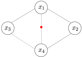
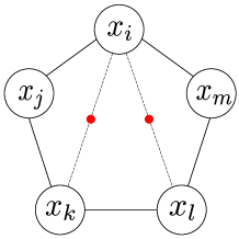
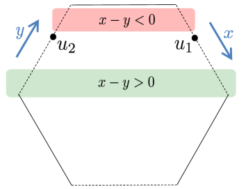
The integrability computation for the five-point functions considered in this work involves the one-particle and the two-particle mirror contributions. More precisely, what we need are the contributions from an one-particle state living on a length-zero bridge and the contributions from two one-particle states living on neighbouring length-zero bridges. See figure 2-(a)𝑎(a) for a pictorial explanation.

The one-particle contribution was computed in [5]. For the configuration depicted in figure 1, the result can be written as666This expression makes manifest the invariance under the flip transformation, zz1𝑧superscript𝑧1z\to z^{-1} and αα1𝛼superscript𝛼1\alpha\to\alpha^{-1}.

(1)(z,α)=m(z)+m(z1),superscript1𝑧𝛼𝑚𝑧𝑚superscript𝑧1\mathcal{M}^{(1)}(z,\alpha)=m(z)+m(z^{-1})\,, (6)

where m(z)𝑚𝑧m(z) is given by

m(z)g2(z+z¯)(α+α¯)2F(1)(z,z¯),𝑚𝑧superscript𝑔2𝑧¯𝑧𝛼¯𝛼2superscript𝐹1𝑧¯𝑧m(z)\equiv g^{2}\frac{(z+\bar{z})-(\alpha+\bar{\alpha})}{2}F^{(1)}(z,\bar{z})\,, (7)

and the cross ratios are defined in (LABEL:eq:TheCrossRatios). As is clear from the definition above, m(z)𝑚𝑧m(z) is actually a function of four cross ratios z𝑧z, z¯¯𝑧\bar{z}, α𝛼\alpha and α¯¯𝛼\bar{\alpha}. We however only write the dependence on the first argument z𝑧z since it is easy to figure out the dependence on the other arguments. F(1)superscript𝐹1F^{(1)} and g𝑔g are defined by

F(1)(z,z¯)Φ(z,z¯)zz¯(=x132x242π2d4x5x152x252x352x452)andg2=λ16π2,formulae-sequencesuperscript𝐹1𝑧¯𝑧annotatedΦ𝑧¯𝑧𝑧¯𝑧absentsuperscriptsubscript𝑥132superscriptsubscript𝑥242superscript𝜋2superscript𝑑4subscript𝑥5superscriptsubscript𝑥152subscriptsuperscript𝑥225subscriptsuperscript𝑥235subscriptsuperscript𝑥245andsuperscript𝑔2𝜆16superscript𝜋2F^{(1)}(z,\bar{z})\equiv\frac{\Phi(z,\bar{z})}{z-\bar{z}}\quad\left(=\frac{x_{13}^{2}x_{24}^{2}}{\pi^{2}}\int\frac{d^{4}x_{5}}{x_{15}^{2}x^{2}_{25}x^{2}_{35}x^{2}_{45}}\right)\,\quad{\rm{and}}\quad g^{2}=\frac{\lambda}{16\pi^{2}}\,, (8)

with λ𝜆\lambda being the ‘t Hooft coupling. The function Φ(z,z¯)Φ𝑧¯𝑧\Phi(z,\bar{z}) is given by

Φ(z,z¯)=2Li2(z)2Li2(z¯)+log(zz¯)log(1z1z¯).Φ𝑧¯𝑧2Lsubscripti2𝑧2Lsubscripti2¯𝑧𝑧¯𝑧1𝑧1¯𝑧\Phi(z,\bar{z})=2{\rm Li}_{2}(z)-2{\rm Li}_{2}(\bar{z})+\log(z\bar{z})\log\left(\frac{1-z}{1-\bar{z}}\right)\,. (9)

The function m(z)𝑚𝑧m(z) has several important properties,

m(0)=m(1)=m()=0,𝑚0𝑚1𝑚0\displaystyle m(0)=m(1)=m(\infty)=0\,, (10)
m(z)+m(1z)=0,𝑚𝑧𝑚1𝑧0\displaystyle m(z)+m(1-z)=0\,,

which we use often in this paper.

Refer to caption
Figure 1: The configuration for the one-particle mirror correction. The dashed line denotes the length-zero bridge while the red dot denotes the mirror particle. The result is given in (6).

The computation of the two-particle contribution is the main outcome of this work and will be explained in section 3. The result turns out to be given by a linear combination of one-loop conformal integrals. For the configuration depicted in figure 2-(a)𝑎(a), the result reads

(2)(z1,z2,α1,α2)=superscript2subscript𝑧1subscript𝑧2subscript𝛼1subscript𝛼2absent\displaystyle\mathcal{M}^{(2)}(z_{1},z_{2},\alpha_{1},\alpha_{2})= m(z1)m(z21)𝑚subscript𝑧1𝑚superscriptsubscript𝑧21\displaystyle-m(z_{1})-m(z_{2}^{-1}) (11)
+m(z11z1z2)+m(1z1+z1z2z2)+m(z1(1z2)),𝑚subscript𝑧11subscript𝑧1subscript𝑧2𝑚1subscript𝑧1subscript𝑧1subscript𝑧2subscript𝑧2𝑚subscript𝑧11subscript𝑧2\displaystyle+m\left(\frac{z_{1}-1}{z_{1}z_{2}}\right)+m\left(\frac{1-z_{1}+z_{1}z_{2}}{z_{2}}\right)+m\left(z_{1}(1-z_{2})\right)\,,

where the cross ratios in the formula are given by

z1z¯1=xim2xkl2xik2xml2,(1z1)(1z¯1)=xil2xkm2xik2xlm2,z2z¯2=xil2xjk2xij2xlk2,(1z2)(1z¯2)=xik2xjl2xij2xkl2,formulae-sequencesubscript𝑧1subscript¯𝑧1superscriptsubscript𝑥𝑖𝑚2superscriptsubscript𝑥𝑘𝑙2superscriptsubscript𝑥𝑖𝑘2superscriptsubscript𝑥𝑚𝑙2formulae-sequence1subscript𝑧11subscript¯𝑧1superscriptsubscript𝑥𝑖𝑙2superscriptsubscript𝑥𝑘𝑚2superscriptsubscript𝑥𝑖𝑘2superscriptsubscript𝑥𝑙𝑚2formulae-sequencesubscript𝑧2subscript¯𝑧2subscriptsuperscript𝑥2𝑖𝑙subscriptsuperscript𝑥2𝑗𝑘subscriptsuperscript𝑥2𝑖𝑗subscriptsuperscript𝑥2𝑙𝑘1subscript𝑧21subscript¯𝑧2superscriptsubscript𝑥𝑖𝑘2superscriptsubscript𝑥𝑗𝑙2subscriptsuperscript𝑥2𝑖𝑗subscriptsuperscript𝑥2𝑘𝑙z_{1}\bar{z}_{1}=\frac{x_{im}^{2}x_{kl}^{2}}{x_{ik}^{2}x_{ml}^{2}}\,,\,\,(1-z_{1})(1-\bar{z}_{1})=\frac{x_{il}^{2}x_{km}^{2}}{x_{ik}^{2}x_{lm}^{2}}\,,\,\,z_{2}\bar{z}_{2}=\frac{x^{2}_{il}x^{2}_{jk}}{x^{2}_{ij}x^{2}_{lk}}\,,\,\,(1-z_{2})(1-\bar{z}_{2})=\frac{x_{ik}^{2}x_{jl}^{2}}{x^{2}_{ij}x^{2}_{kl}}\,, (12)

and similarly for the R𝑅R-charge cross-ratios α1subscript𝛼1\alpha_{1} and α2subscript𝛼2\alpha_{2}.

Refer to caption
Refer to caption
Refer to caption

(a)𝑎(a)

(b)𝑏(b)

(c)𝑐(c)

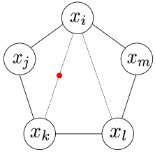
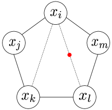
Figure 2: The two-particle mirror correction, (a)𝑎(a), and the related one-particle corrections, (b)𝑏(b) and (c)𝑐(c). The red dots are the mirror particles and the dashed lines are zero length bridges. The sum of three contributions gives a one-loop correction to the decagon and is given by a simple combination of the one-loop conformal integrals as shown in (13).

One can then compute the sum of the one-particle and the two-particle corrections that contribute to the decagon depicted in figure 2 as follows:

(1)(z1,α1)+(1)(z2,α2)+(2)(z1,z2,α1,α2)=superscript1subscript𝑧1subscript𝛼1superscript1subscript𝑧2subscript𝛼2superscript2subscript𝑧1subscript𝑧2subscript𝛼1subscript𝛼2absent\displaystyle\mathcal{M}^{(1)}(z_{1},\alpha_{1})+\mathcal{M}^{(1)}(z_{2},\alpha_{2})+\mathcal{M}^{(2)}(z_{1},z_{2},\alpha_{1},\alpha_{2})= (13)
m(z11)+m(z2)+m(z11z1z2)+m(1z1+z1z2z2)+m(z1(1z2)).𝑚superscriptsubscript𝑧11𝑚subscript𝑧2𝑚subscript𝑧11subscript𝑧1subscript𝑧2𝑚1subscript𝑧1subscript𝑧1subscript𝑧2subscript𝑧2𝑚subscript𝑧11subscript𝑧2\displaystyle m(z_{1}^{-1})+m(z_{2})+m\left(\frac{z_{1}-1}{z_{1}z_{2}}\right)+m\left(\frac{1-z_{1}+z_{1}z_{2}}{z_{2}}\right)+m\left(z_{1}(1-z_{2})\right)\,.

An important property of this expression is that the five terms in the formula correspond to all possible cross ratios that can be formed inside the five-point graph depicted in figure 2. This makes it clear that the result is independent of the way we cut the graph into hexagons. This property, called the flip invariance, will be discussed more in detail in section 3.2.

In the following two subsections, we show that one can reproduce the perturbative data for five-point functions from these expressions.

2.3 Comparison I: Five 20

Let us first study the simplest five-point functions, which is the correlator of five length-two operators (also known as 20superscript2020^{\prime} operators).

To express the perturbative result, we introduce the definitions

sijkl=xij2xkl2xik2xjl2zijklz¯ijkl,tijkl=xil2xjk2xik2xjl2(1zijkl)(1z¯ijkl).formulae-sequencesubscript𝑠𝑖𝑗𝑘𝑙subscriptsuperscript𝑥2𝑖𝑗subscriptsuperscript𝑥2𝑘𝑙subscriptsuperscript𝑥2𝑖𝑘subscriptsuperscript𝑥2𝑗𝑙subscript𝑧𝑖𝑗𝑘𝑙subscript¯𝑧𝑖𝑗𝑘𝑙subscript𝑡𝑖𝑗𝑘𝑙subscriptsuperscript𝑥2𝑖𝑙subscriptsuperscript𝑥2𝑗𝑘subscriptsuperscript𝑥2𝑖𝑘subscriptsuperscript𝑥2𝑗𝑙1subscript𝑧𝑖𝑗𝑘𝑙1subscript¯𝑧𝑖𝑗𝑘𝑙s_{ijkl}=\frac{x^{2}_{ij}x^{2}_{kl}}{x^{2}_{ik}x^{2}_{jl}}\equiv z_{ijkl}\,\bar{z}_{ijkl}\,,\quad\quad t_{ijkl}=\frac{x^{2}_{il}x^{2}_{jk}}{x^{2}_{ik}x^{2}_{jl}}\equiv(1-z_{ijkl})(1-\bar{z}_{ijkl})\,. (14)

and

Dijkl=g2F(1)(zijkl,z¯ijkl)(2dikdjl+(sijkl1tijkl)dildjk+(tijkl1sijkl)dijdkl),subscript𝐷𝑖𝑗𝑘𝑙superscript𝑔2superscript𝐹1subscript𝑧𝑖𝑗𝑘𝑙subscript¯𝑧𝑖𝑗𝑘𝑙2subscript𝑑𝑖𝑘subscript𝑑𝑗𝑙subscript𝑠𝑖𝑗𝑘𝑙1subscript𝑡𝑖𝑗𝑘𝑙subscript𝑑𝑖𝑙subscript𝑑𝑗𝑘subscript𝑡𝑖𝑗𝑘𝑙1subscript𝑠𝑖𝑗𝑘𝑙subscript𝑑𝑖𝑗subscript𝑑𝑘𝑙D_{ijkl}=g^{2}F^{(1)}(z_{ijkl},\bar{z}_{ijkl})(2d_{ik}d_{jl}+(s_{ijkl}-1-t_{ijkl})d_{il}d_{jk}+(t_{ijkl}-1-s_{ijkl})d_{ij}d_{kl})\,, (15)

which can also be written in terms of m(z)𝑚𝑧m(z) as

Dijkl=2m(zijlk)dildjk+2m(ziljk)dijdlk.subscript𝐷𝑖𝑗𝑘𝑙2𝑚subscript𝑧𝑖𝑗𝑙𝑘subscript𝑑𝑖𝑙subscript𝑑𝑗𝑘2𝑚subscript𝑧𝑖𝑙𝑗𝑘subscript𝑑𝑖𝑗subscript𝑑𝑙𝑘D_{ijkl}=2m(z_{ijlk})d_{il}d_{jk}+2m(z_{iljk})d_{ij}d_{lk}\,. (16)

Then the one-loop result in [8] can be expressed as

G{2,2,2,2,2}1|perturbation=evaluated-atsubscriptsuperscript𝐺122222perturbation\displaystyle\left.G^{1}_{\{2,2,2,2,2\}}\right|_{\rm perturbation}=- (D1234[1 3,2 4|5]+D1324[1 2,3 4|5]+D1243[1 4,2 3|5]\displaystyle\left(D_{1234}[1\,3,2\,4|5]+D_{1324}[1\,2,3\,4|5]+D_{1243}[1\,4,2\,3|5]\right. (17)
+D1235[1 3,2 5|4]+D1325[1 2,5 3|4]+D1253[1 5,2 3|4]subscript𝐷123513conditional254subscript𝐷132512conditional534subscript𝐷125315conditional234\displaystyle+D_{1235}[1\,3,2\,5|4]+D_{1325}[1\,2,5\,3|4]+D_{1253}[1\,5,2\,3|4]
+D1254[1 5,2 4|3]+D1524[1 2,4 5|3]+D1245[1 4,2 5|3]subscript𝐷125415conditional243subscript𝐷152412conditional453subscript𝐷124514conditional253\displaystyle+D_{1254}[1\,5,2\,4|3]+D_{1524}[1\,2,4\,5|3]+D_{1245}[1\,4,2\,5|3]
+D1534[1 3,5 4|2]+D1354[1 5,3 4|2]+D1543[1 4,5 3|2]subscript𝐷153413conditional542subscript𝐷135415conditional342subscript𝐷154314conditional532\displaystyle+D_{1534}[1\,3,5\,4|2]+D_{1354}[1\,5,3\,4|2]+D_{1543}[1\,4,5\,3|2]
+D5234[5 3,2 4|1]+D5324[5 2,3 4|1]+D5243[5 4,2 3|1]).\displaystyle\left.+D_{5234}[5\,3,2\,4|1]+D_{5324}[5\,2,3\,4|1]+D_{5243}[5\,4,2\,3|1]\right)\;.

Here G{Li}1subscriptsuperscript𝐺1subscript𝐿𝑖G^{1}_{\{L_{i}\}} is the one-loop correction to the connected correlator defined in (2.1) and [ij,kl|m]𝑖𝑗conditional𝑘𝑙𝑚[ij,kl|m] is given by

[ij,kl|m]=dimdjmdkl+dijdkmdlm.𝑖𝑗conditional𝑘𝑙𝑚subscript𝑑𝑖𝑚subscript𝑑𝑗𝑚subscript𝑑𝑘𝑙subscript𝑑𝑖𝑗subscript𝑑𝑘𝑚subscript𝑑𝑙𝑚[i\,j,k\,l|m]=d_{im}\,d_{jm}\,d_{kl}+d_{ij}\,d_{km}\,d_{lm}\,. (18)

We now explain how to reproduce the result above from the hexagonalization procedure. The general rule of the hexagonalization is that for a n𝑛n-point correlation function, one needs 2(n2)2𝑛22(n-2) hexagons. Thus for n𝑛n=5 one needs to decompose the surface into six hexagonal patches. The first step in the calculation is to enumerate the Wick contractions at tree level. At tree level, one has the following twelve graphs:

G{2,2,2,2,2}0=d12d24d43d35d51+d12d23d34d45d51+d12d25d53d34d41subscriptsuperscript𝐺022222subscript𝑑12subscript𝑑24subscript𝑑43subscript𝑑35subscript𝑑51subscript𝑑12subscript𝑑23subscript𝑑34subscript𝑑45subscript𝑑51subscript𝑑12subscript𝑑25subscript𝑑53subscript𝑑34subscript𝑑41\displaystyle G^{0}_{\{2,2,2,2,2\}}=d_{12}d_{24}d_{43}d_{35}d_{51}+d_{12}d_{23}d_{34}d_{45}d_{51}+d_{12}d_{25}d_{53}d_{34}d_{41} (19)
+d12d23d35d54d41+d12d25d54d43d31+d12d24d45d53d31subscript𝑑12subscript𝑑23subscript𝑑35subscript𝑑54subscript𝑑41subscript𝑑12subscript𝑑25subscript𝑑54subscript𝑑43subscript𝑑31subscript𝑑12subscript𝑑24subscript𝑑45subscript𝑑53subscript𝑑31\displaystyle+\,d_{12}d_{23}d_{35}d_{54}d_{41}+d_{12}d_{25}d_{54}d_{43}d_{31}+d_{12}d_{24}d_{45}d_{53}d_{31}
+d13d34d42d25d51+d13d32d24d45d51+d13d35d52d24d41subscript𝑑13subscript𝑑34subscript𝑑42subscript𝑑25subscript𝑑51subscript𝑑13subscript𝑑32subscript𝑑24subscript𝑑45subscript𝑑51subscript𝑑13subscript𝑑35subscript𝑑52subscript𝑑24subscript𝑑41\displaystyle+\,d_{13}d_{34}d_{42}d_{25}d_{51}+d_{13}d_{32}d_{24}d_{45}d_{51}+d_{13}d_{35}d_{52}d_{24}d_{41}
+d13d32d25d54d41+d14d43d32d25d51+d14d42d23d35d51.subscript𝑑13subscript𝑑32subscript𝑑25subscript𝑑54subscript𝑑41subscript𝑑14subscript𝑑43subscript𝑑32subscript𝑑25subscript𝑑51subscript𝑑14subscript𝑑42subscript𝑑23subscript𝑑35subscript𝑑51\displaystyle+\,d_{13}d_{32}d_{25}d_{54}d_{41}+d_{14}d_{43}d_{32}d_{25}d_{51}+d_{14}d_{42}d_{23}d_{35}d_{51}\,.
Refer to caption
Figure 3: All the mirror particles contributions for the graph corresponding to the first term in (19).

The second step is to decompose each tree-level graph into six hexagons and dress it with mirror particles. Important simplifications at one loop are:

  1. 1.

    Only single-particle states on zero-length bridges can contribute.

  2. 2.

    Whenever one introduces more than one particle, they must always be neighbors; namely each of them must share at least one hexagon with some other magnons.

These rules follow simply from the following weak-coupling behavior of the one-particle measure, the mirror energy and the hexagon form factor:

μO(g2),eE~O(g2),𝔥(uγ,vγ)O(1/g2).formulae-sequencesimilar-to𝜇𝑂superscript𝑔2formulae-sequencesimilar-tosuperscript𝑒~𝐸𝑂superscript𝑔2similar-to𝔥superscript𝑢𝛾superscript𝑣𝛾𝑂1superscript𝑔2\displaystyle\mu\sim O(g^{2})\,,\quad\quad e^{-\tilde{E}}\sim O(g^{2})\,,\quad\quad\mathfrak{h}(u^{\gamma},v^{-\gamma})\sim O(1/g^{2})\,. (20)

The first two equalities show that we can only have single-particle states on zero-length bridges. The last equality explains why we can have multi-particle contributions: If we just take into account the measure factor μ𝜇\mu, the n(>1)annotated𝑛absent1n(>1) particle contributions seem to appear at O(g2n)𝑂superscript𝑔2𝑛O(g^{2n}). However they get enhanced because of the interaction, 𝔥(uγ,vγ)𝔥superscript𝑢𝛾superscript𝑣𝛾\mathfrak{h}(u^{\gamma},v^{-\gamma}).

Now, for definiteness, let us consider the graph corresponding to the first term in (19). All the one-loop mirror-particle contributions for this case are depicted in figure 3. Summing them up, one gets the result777The way to find the arguments of the functions (1)superscript1\mathcal{M}^{(1)} and (2)superscript2\mathcal{M}^{(2)} follows from (12). Here we give further details in how to find them. Consider the second diagram of figure 3. The spacetime argument of (1)superscript1\mathcal{M}^{(1)} for this contribution is found by replacing x1=0,x3=1,x4=formulae-sequencesubscript𝑥10formulae-sequencesubscript𝑥31subscript𝑥4x_{1}=0,x_{3}=1,x_{4}=\infty in the formulas for the cross ratios (LABEL:eq:TheCrossRatios) and solving for the holomorphic part of x2subscript𝑥2x_{2}. Similarly, to read the argument for the first diagram of the figure, one sets x1=0,x5=1,x3=formulae-sequencesubscript𝑥10formulae-sequencesubscript𝑥51subscript𝑥3x_{1}=0,x_{5}=1,x_{3}=\infty and solves for the holomorphic part of x4subscript𝑥4x_{4}. Finally, the arguments of the function (2)superscript2\mathcal{M}^{(2)} are the same for the one particle and they are read counterclockwise. ,

H12435=subscript𝐻12435absent\displaystyle H_{12435}=  2d12d24d43d35d51[(1)(z,α)+(1)(1w1,1β1)\displaystyle\,2d_{12}d_{24}d_{43}d_{35}d_{51}\Big{[}\mathcal{M}^{(1)}(z,\alpha)+\mathcal{M}^{(1)}(1-w^{-1},1-\beta^{-1}) (21)
+(2)(z,1w1,α,1β1)].\displaystyle\quad\,+\mathcal{M}^{(2)}(z,1-w^{-1},\alpha,1-\beta^{-1})\Big{]}\,.

Using (13), one can express it in terms of m(z)𝑚𝑧m(z) as follows888To compare with the perturbative result, it is also useful to express (23) in terms of the cross ratios zijklsubscript𝑧𝑖𝑗𝑘𝑙z_{ijkl} as follows: H12435=2d12d24d43d35d51[m(z1324)+m(z2543)+m(z4135)+m(z3251)+m(z5412)].subscript𝐻124352subscript𝑑12subscript𝑑24subscript𝑑43subscript𝑑35subscript𝑑51delimited-[]𝑚subscript𝑧1324𝑚subscript𝑧2543𝑚subscript𝑧4135𝑚subscript𝑧3251𝑚subscript𝑧5412H_{12435}=2d_{12}d_{24}d_{43}d_{35}d_{51}\left[m(z_{1324})+m(z_{2543})+m(z_{4135})+m(z_{3251})+m(z_{5412})\right]\,. (22) :

H12435=subscript𝐻12435absent\displaystyle H_{12435}= 2d12d24d43d35d51×\displaystyle 2d_{12}d_{24}d_{43}d_{35}d_{51}\times (23)
[m(z1)+m(1w1)+m(1z11w1)+m(zw1w)+m(zw)].delimited-[]𝑚superscript𝑧1𝑚1superscript𝑤1𝑚1superscript𝑧11superscript𝑤1𝑚𝑧𝑤1𝑤𝑚𝑧𝑤\displaystyle\left[m(z^{-1})+m(1-w^{-1})+m\left(\frac{1-z^{-1}}{1-w^{-1}}\right)+m\left(\frac{z-w}{1-w}\right)+m\left(\frac{z}{w}\right)\right]\,.

The full integrability result is obtained by adding the contributions for all twelve tree-level graphs:

G{2,2,2,2,2}1|integrabilityevaluated-atsubscriptsuperscript𝐺122222integrability\displaystyle\left.G^{1}_{\{2,2,2,2,2\}}\right|_{\rm integrability} =H12435+H12345+H12534+H12354+H12543+H12453absentsubscript𝐻12435subscript𝐻12345subscript𝐻12534subscript𝐻12354subscript𝐻12543subscript𝐻12453\displaystyle=H_{12435}+H_{12345}+H_{12534}+H_{12354}+H_{12543}+H_{12453} (24)
+H13425+H13245+H13524+H13254+H14325+H14235.subscript𝐻13425subscript𝐻13245subscript𝐻13524subscript𝐻13254subscript𝐻14325subscript𝐻14235\displaystyle+H_{13425}+H_{13245}+H_{13524}+H_{13254}+H_{14325}+H_{14235}\,.

Adding all the terms and using the properties of m(z)𝑚𝑧m(z) (10), we find that the answer perfectly matches the perturbative result (17).

Note that, although here we chose one particular way of decomposing the five-point function into hexagons, the final result is independent of the way we decompose it. This “flip invariance” is an important consistency check of our results and it will be discussed in section 3.

2.4 Comparison II: Three L=2𝐿2L=2 and two L=3𝐿3L=3 BPS operators

In this section, we compute the correlation function of three length-two and two length-three BPS operators using integrability. For definiteness, we choose the fourth and the fifth operators to be the length-three operators.
Refer to caption
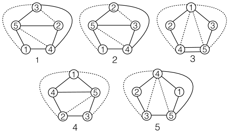
Figure 4: Graphs that contribute to the correlation function of three L=2𝐿2L=2 and two L=3𝐿3L=3 BPS operators. The full set of graphs is obtained by permuting the operators 1,2121,2 and 333 in the diagrams 3,4343,4 and 555 above. The one-loop result is obtained by adding both the one- and two-particle contributions associated with the zero-length bridges (dashed lines).

For this correlator, the one-loop perturbative result in [8] reads (in our conventions)

G{2,2,2,3,3}1(x1,x2,x3,x4,x5)|perturbation=evaluated-atsubscriptsuperscript𝐺122233subscript𝑥1subscript𝑥2subscript𝑥3subscript𝑥4subscript𝑥5perturbationabsent\displaystyle\left.G^{1}_{\{2,2,2,3,3\}}(x_{1},x_{2},x_{3},x_{4},x_{5})\right|_{\rm perturbation}= (25)
d45G{2,2,2,2,2}1(x1,x2,x3,x4,x5)+d14d15G{2,2,2,2}1(x2,x3,x4,x5)subscript𝑑45subscriptsuperscript𝐺122222subscript𝑥1subscript𝑥2subscript𝑥3subscript𝑥4subscript𝑥5subscript𝑑14subscript𝑑15subscriptsuperscript𝐺12222subscript𝑥2subscript𝑥3subscript𝑥4subscript𝑥5\displaystyle\qquad d_{45}G^{1}_{\{2,2,2,2,2\}}(x_{1},x_{2},x_{3},x_{4},x_{5})+d_{14}d_{15}G^{1}_{\{2,2,2,2\}}(x_{2},x_{3},x_{4},x_{5})
+d24d25G{2,2,2,2}1(x1,x3,x4,x5)+d34d35G{2,2,2,2}1(x1,x2,x4,x5),subscript𝑑24subscript𝑑25subscriptsuperscript𝐺12222subscript𝑥1subscript𝑥3subscript𝑥4subscript𝑥5subscript𝑑34subscript𝑑35subscriptsuperscript𝐺12222subscript𝑥1subscript𝑥2subscript𝑥4subscript𝑥5\displaystyle\qquad+d_{24}d_{25}G^{1}_{\{2,2,2,2\}}(x_{1},x_{3},x_{4},x_{5})+d_{34}d_{35}G^{1}_{\{2,2,2,2\}}(x_{1},x_{2},x_{4},x_{5})\,,

where G{2,2,2,2}1subscriptsuperscript𝐺12222G^{1}_{\{2,2,2,2\}} is given by

G{2,2,2,2}1(xi,xj,xk,xl)=DijkldikdjlDijlkdildjkDikjldijdkl.subscriptsuperscript𝐺12222subscript𝑥𝑖subscript𝑥𝑗subscript𝑥𝑘subscript𝑥𝑙subscript𝐷𝑖𝑗𝑘𝑙subscript𝑑𝑖𝑘subscript𝑑𝑗𝑙subscript𝐷𝑖𝑗𝑙𝑘subscript𝑑𝑖𝑙subscript𝑑𝑗𝑘subscript𝐷𝑖𝑘𝑗𝑙subscript𝑑𝑖𝑗subscript𝑑𝑘𝑙G^{1}_{\{2,2,2,2\}}(x_{i},x_{j},x_{k},x_{l})=-D_{ijkl}d_{ik}d_{jl}-D_{ijlk}d_{il}d_{jk}-D_{ikjl}d_{ij}d_{kl}\,. (26)

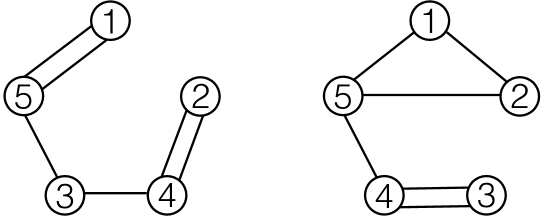
To reproduce this result from integrability, one first list up the connected tree-level diagrams and then decompose them into hexagons. The connected tree-level diagrams are divided into two sets, 1-edge irreducible (1EI) graphs and non-1EI graphs [5]. The 1EI graphs are graphs that are still connected when any one of its non-zero length bridges are cut. For the specific correlation function that we are considering, examples of 1EI graphs and of non-1EI are given in the figures 4 and 5 respectively. In [5], we proposed that one only needs to consider the corrections coming from 1EI graphs in order to compute the correlation functions of the BPS operators. In other words, we expect that the mirror-particle corrections coming from non-1EI graphs add up to zero. We have not been able to show this cancellation explicitly for the graphs in figure 5 since, for that purpose, one needs more than two-particle contributions. However, we show in section 4 that such cancellation indeed takes place for next-to-extremal four-point functions. In what follows, we compute the one-loop five-point function assuming that the non-1EI graphs do not contribute.
Refer to caption
Figure 5: Two examples of non-1EI graphs. The contributions coming from these types of graphs are expected to be zero.

The 1EI graphs relevant for the correlation function of three length-two and two length-three BPS operators are shown in figure 4. The complete set of graphs is composed of the diagrams 1 and 2 and of all the permutations of the operators 1, 2 and 3 of the diagrams 3, 4 and 5. At one loop, one has to compute the one-particle and two-particles contributions associated with the zero-length bridges. From the diagrams 111 and 222, we get

Diagram 1+Diagram 2=d41d15d53d34d42d25×\displaystyle{\rm Diagram}\,1+{\rm Diagram}\,2\,=\,d_{41}d_{15}d_{53}d_{34}d_{42}d_{25}\,\times (27)
[2(1)(1zw,1αβ)+2(1)(wzw1,βαβ1)+2(1)(1w1,1β1)].delimited-[]2superscript11𝑧𝑤1𝛼𝛽2superscript1𝑤𝑧𝑤1𝛽𝛼𝛽12superscript11superscript𝑤11superscript𝛽1\displaystyle\left[2\mathcal{M}^{(1)}\left(1-\frac{z}{w},1-\frac{\alpha}{\beta}\right)+2\mathcal{M}^{(1)}\left(\frac{w-z}{w-1},\frac{\beta-\alpha}{\beta-1}\right)+2\,\mathcal{M}^{(1)}\left(1-w^{-1},1-\beta^{-1}\right)\,\right]\,.

The diagram 3 is similar to the diagrams that appeared in the previous subsection, see figure 3; the only difference is that it has one more propagator:

Diagram 3=d45H13542.Diagram3subscript𝑑45subscript𝐻13542\displaystyle{\rm Diagram}\,3=\,d_{45}H_{13542}\,. (28)

Lastly, the diagrams 444 and 555 give

Diagrams 4+Diagrams 5=d14d45d51d42d23d35×\displaystyle{\rm{Diagrams}}\,4+{\rm{Diagrams}}\,5\,=\,d_{14}d_{45}d_{51}d_{42}d_{23}d_{35}\,\times (29)
[ 3(1)(w1z1,β1α1)+(1)(1z,1α)+(1)(1w1,1β1)\displaystyle\left[\,3\,\mathcal{M}^{(1)}\left(\frac{w-1}{z-1},\frac{\beta-1}{\alpha-1}\right)+\,\mathcal{M}^{(1)}\left(1-z,1-\alpha\right)+\,\mathcal{M}^{(1)}\left(1-w^{-1},1-\beta^{-1}\right)\right.
+(1)(z(w1)w(z1),α(β1)β(α1))+(2)(1z,z(w1)w(z1))+(2)(1w1,z1w1)].\displaystyle\left.+\,\mathcal{M}^{(1)}\left(\frac{z(w-1)}{w(z-1)},\frac{\alpha(\beta-1)}{\beta(\alpha-1)}\right)+\mathcal{M}^{(2)}\left(1-z,\frac{z(w-1)}{w(z-1)}\right)+\mathcal{M}^{(2)}\left(1-w^{-1},\frac{z-1}{w-1}\right)\right]\,.

Adding all the diagrams (including the permutations), one can reproduce the perturbative result given in (LABEL:eq:TheFive22233). This supports our original assumption that the sum of the mirror-particle corrections for non-1EI graphs vanishes.

3 Two-Particle Contributions and Flip Invariance

We now outline how to compute the two-particle contribution shown in figure 2 to get (11). More technical details are explained in Appendices B and D. In addition, we discuss the flip invariance of the two-particle result.

3.1 The Two-Particle Computation

To compute the two-particle contribution given in figure 2, one has to evaluate the contribution from each hexagon and sum over all the mirror particle bound states which we insert on the dashed edges.

Let us begin by recalling what the mirror-particle states are. A complete basis of states on the mirror edge is given by multi-particle states made up of various bound states. Each bound state is labelled by the integer a𝑎a, and the a𝑎a-th mirror bound state 𝒳𝒳\mathcal{X} is made up of a pair of “quarks” χ𝜒\chi and χ˙˙𝜒\dot{\chi}, each of which belongs to the a𝑎a-th anti-symmetric representation of 𝔰𝔲(2|2)𝔰𝔲conditional22\mathfrak{su}(2|2):

χ,χ˙=𝜒˙𝜒absent\displaystyle\chi\,,\,\,\dot{\chi}= |ψα1ψαa+,ketsubscript𝜓subscript𝛼1subscript𝜓subscript𝛼𝑎\displaystyle|\psi_{\alpha_{1}}\cdots\psi_{\alpha_{a}}\rangle+\cdots\,,\quad |ϕ1ψa1ψαa1+,ketsubscriptitalic-ϕ1subscript𝜓subscript𝑎1subscript𝜓subscript𝛼𝑎1\displaystyle|\phi_{1}\psi_{a_{1}}\cdots\psi_{\alpha_{a-1}}\rangle+\cdots\,, (30)
|ϕ2ψα1ψαa1+.ketsubscriptitalic-ϕ2subscript𝜓subscript𝛼1subscript𝜓subscript𝛼𝑎1\displaystyle|\phi_{2}\psi_{\alpha_{1}}\cdots\psi_{\alpha_{a-1}}\rangle+\cdots.\quad |ϕ1ϕ2ψα1ψαa2+.ketsubscriptitalic-ϕ1subscriptitalic-ϕ2subscript𝜓subscript𝛼1subscript𝜓subscript𝛼𝑎2\displaystyle|\phi_{1}\phi_{2}\psi_{\alpha_{1}}\cdots\psi_{\alpha_{a-2}}\rangle+\cdots.

A small complication which arises for the multi-point functions is that the naive basis given above does not reproduce the correct perturbative result. To obtain a match, one needs to dress the basis elements with the so-called Z𝑍Z-markers as follows [5]:

|ψα1ψαa+,ketsubscript𝜓subscript𝛼1subscript𝜓subscript𝛼𝑎\displaystyle|\psi_{\alpha_{1}}\cdots\psi_{\alpha_{a}}\rangle+\cdots\,,\quad |Z±12ϕ1ψa1ψαa1+,ketsuperscript𝑍plus-or-minus12subscriptitalic-ϕ1subscript𝜓subscript𝑎1subscript𝜓subscript𝛼𝑎1\displaystyle|Z^{\pm\frac{1}{2}}\phi_{1}\psi_{a_{1}}\cdots\psi_{\alpha_{a-1}}\rangle+\cdots\,, (31)
|Z12ϕ2ψα1ψαa1+.ketsuperscript𝑍minus-or-plus12subscriptitalic-ϕ2subscript𝜓subscript𝛼1subscript𝜓subscript𝛼𝑎1\displaystyle|Z^{\mp\frac{1}{2}}\phi_{2}\psi_{\alpha_{1}}\cdots\psi_{\alpha_{a-1}}\rangle+\cdots.\quad |ϕ1ϕ2ψα1ψαa2+,ketsubscriptitalic-ϕ1subscriptitalic-ϕ2subscript𝜓subscript𝛼1subscript𝜓subscript𝛼𝑎2\displaystyle|\phi_{1}\phi_{2}\psi_{\alpha_{1}}\cdots\psi_{\alpha_{a-2}}\rangle+\cdots,

The correct result is reproduced after one averages over the two signs. This was shown explicitly for the one-particle contribution in [5]. Also for the two-particle contribition, we found that essentially the same prescription (with a little bit of refinement) gives the correct answer. For details of the prescription, see Appendix A.
Refer to caption
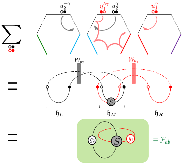
Figure 6: The matrix part for the two-particle contribution. The top line explains how we compute it using the hexagon formalism: We rewrite the middle hexagon by performing the 5γ5𝛾5\gamma-mirror transformation to the first particle. The second line shows the pictorial representation of the matrix part: The summation over the flavor indices corresponds to adding dashed curves in the figure, and 𝒲uisubscript𝒲subscript𝑢𝑖\mathcal{W}_{u_{i}}’s are the weight factors. The last line gives the final result for the matrix part and the definition of absubscript𝑎𝑏\mathcal{F}_{ab}: It is essentially given by two intersecting loops. At the intersection point we insert the 𝔰𝔲(2|2)𝔰𝔲conditional22\mathfrak{su}(2|2) S-matrix (denoted by a gray dot in the figure) and, on each loop, we insert a twist gisubscript𝑔𝑖g_{i}. The twist comes from the insertion of the weight factor 𝒲uisubscript𝒲subscript𝑢𝑖\mathcal{W}_{u_{i}} and it produces different phases depending on the flavors. (See also [5]).

Having determined the correct basis elements, one can write down999One also needs to average over the choices of the signs in (31), although we did not write it explicitly here. the two-particle contribution following the general prescription given in [5]:

(2)(z1,z2,α1,α2)=du12πdu22πa=1b=1μa(u1γ)μb(u2γ)IJsuperscript2subscript𝑧1subscript𝑧2subscript𝛼1subscript𝛼2𝑑subscript𝑢12𝜋𝑑subscript𝑢22𝜋superscriptsubscript𝑎1superscriptsubscript𝑏1subscript𝜇𝑎superscriptsubscript𝑢1𝛾subscript𝜇𝑏superscriptsubscript𝑢2𝛾subscript𝐼subscript𝐽\displaystyle\mathcal{M}^{(2)}(z_{1},z_{2},\alpha_{1},\alpha_{2})=\int\frac{du_{1}}{2\pi}\frac{du_{2}}{2\pi}\,\sum_{a=1}^{\infty}\sum_{b=1}^{\infty}\mu_{a}(u_{1}^{\gamma})\mu_{b}(u_{2}^{\gamma})\sum_{I}\sum_{J} (32)
𝔥L[𝒳¯b(u2γ)J]𝒲[𝒳b(u2γ)J]𝔥M[𝒳b(u2γ)J𝒳¯a(u1γ)I]𝒲[𝒳a(u1γ)I]𝔥R[𝒳a(u1γ)I],subscript𝔥𝐿delimited-[]subscript¯𝒳𝑏subscriptsuperscriptsubscript𝑢2𝛾𝐽𝒲delimited-[]subscript𝒳𝑏subscriptsuperscriptsubscript𝑢2𝛾𝐽subscript𝔥𝑀delimited-[]subscript𝒳𝑏subscriptsuperscriptsubscript𝑢2𝛾𝐽subscript¯𝒳𝑎subscriptsuperscriptsubscript𝑢1𝛾𝐼𝒲delimited-[]subscript𝒳𝑎subscriptsuperscriptsubscript𝑢1𝛾𝐼subscript𝔥𝑅delimited-[]subscript𝒳𝑎subscriptsuperscriptsubscript𝑢1𝛾𝐼\displaystyle\mathfrak{h}_{L}\left[\bar{\mathcal{X}}_{b}(u_{2}^{-\gamma})_{J}\right]\,\mathcal{W}\left[\mathcal{X}_{b}(u_{2}^{\gamma})_{J}\right]\,\mathfrak{h}_{M}\left[\mathcal{X}_{b}(u_{2}^{\gamma})_{J}\,\bar{\mathcal{X}}_{a}(u_{1}^{-\gamma})_{I}\right]\,\mathcal{W}\left[\mathcal{X}_{a}(u_{1}^{\gamma})_{I}\right]\,\mathfrak{h}_{R}\left[\mathcal{X}_{a}(u_{1}^{\gamma})_{I}\right]\,,

Here 𝔥𝔥\mathfrak{h} denote the hexagon form factors and the subscripts L,M𝐿𝑀L,M and R𝑅R mean the left hexagon, the middle hexagon and the right hexagon respectively, see figure 2. 𝒲𝒲\mathcal{W}’s are the weight factors which incorporate the cross-ratio dependence and μ𝜇\mu’s are the measures. There are two bound state indices a𝑎a and b𝑏b corresponding to the mirror particles 111 and 222. The indices I𝐼I and J𝐽J label the states inside the bound-state module a𝑎a and b𝑏b respectively.

The expression (32) by itself is not very useful for the actual computation. In what follows, we explain the individual factors and derive a more compact form of the two-particle integrand. Let us first discuss the weight factors 𝒲𝒲\mathcal{W}. As discussed in [5], they are determined by the symmetry arguments and consist of the a flavor-independent and a flavor-dependent part. The flavor-independent part is given by

𝖫𝖫{\sf L} 𝖱𝖱{\sf R}
ψ1superscript𝜓1\psi^{1} +1212+\frac{1}{2} 00
ψ2superscript𝜓2\psi^{2} 1212-\frac{1}{2} 00
ϕ1superscriptitalic-ϕ1\phi^{1} 00 +1212+\frac{1}{2}
ϕ2superscriptitalic-ϕ2\phi^{2} 00 1212-\frac{1}{2}
𝖫𝖫{\sf L} 𝖱𝖱{\sf R}
ψ1˙superscript𝜓˙1\psi^{\dot{1}} 1212-\frac{1}{2} 00
ψ2˙superscript𝜓˙2\psi^{\dot{2}} +1212+\frac{1}{2} 00
ϕ1˙superscriptitalic-ϕ˙1\phi^{\dot{1}} 00 1212-\frac{1}{2}
ϕ2˙superscriptitalic-ϕ˙2\phi^{\dot{2}} 00 +1212+\frac{1}{2}
Table 1: The charges of a fundamental magnon under the spacetime and the R-symmetry rotations 𝖫𝖫{\sf L} and 𝖱𝖱{\sf R}.
𝒲nonflavor[𝒳(uiγ)]=e2ip~uilog|zi|,subscript𝒲nonflavordelimited-[]𝒳superscriptsubscript𝑢𝑖𝛾superscript𝑒2𝑖subscript~𝑝subscript𝑢𝑖logsubscript𝑧𝑖\mathcal{W}_{{\rm{non-flavor}}}\left[\mathcal{X}(u_{i}^{\gamma})\right]=e^{-2i\tilde{p}_{u_{i}}{\rm{log}}\,|z_{i}|}\,, (33)

where p~uisubscript~𝑝subscript𝑢𝑖\tilde{p}_{u_{i}} is the mirror momentum, while the flavor-dependent part is given by

𝒲flavor[𝒳]=eiJ𝒳φieiL𝒳ϕieiR𝒳θi,subscript𝒲flavordelimited-[]𝒳superscript𝑒𝑖subscript𝐽𝒳subscript𝜑𝑖superscript𝑒𝑖subscript𝐿𝒳subscriptitalic-ϕ𝑖superscript𝑒𝑖subscript𝑅𝒳subscript𝜃𝑖\mathcal{W}_{{\rm{flavor}}}\left[\mathcal{X}\right]=e^{iJ_{\mathcal{X}}\varphi_{i}}\,e^{iL_{\mathcal{X}}\phi_{i}}\,e^{iR_{\mathcal{X}}\theta_{i}}\,, (34)

where J𝒳subscript𝐽𝒳J_{\mathcal{X}}, L𝒳subscript𝐿𝒳L_{\mathcal{X}} and R𝒳subscript𝑅𝒳R_{\mathcal{X}} are the eigenvalues of the state 𝒳𝒳\mathcal{X} for the generators J𝐽J, L𝐿L, and R𝑅R defined below101010The fact that only the generators L𝐿L, R𝑅R and J𝐽J enter in the weight factor is a consequence of our special kinematics: If the operators are not contained in a single two-dimensional plane, one would need other generators which move the operators away from that two-dimensional plane. :

J:eiJφZ=eiφZ,eiJφZ¯=eiφZ¯,L=12(L 11L 22L1˙1˙+L2˙2˙),R=12(R 11R 22R1˙1˙+R2˙2˙),\displaystyle\begin{aligned} &J:\quad e^{iJ\varphi}Z=e^{i\varphi}Z\,,\qquad e^{iJ\varphi}\bar{Z}=e^{-i\varphi}\bar{Z}\,,\\ &L=\frac{1}{2}(L^{1}_{\;1}-L^{2}_{\;2}-L^{\dot{1}}_{\;\dot{1}}+L^{\dot{2}}_{\;\dot{2}})\,,\quad\quad R=\frac{1}{2}(R^{1}_{\;1}-R^{2}_{\;2}-R^{\dot{1}}_{\;\dot{1}}+R^{\dot{2}}_{\;\dot{2}})\,,\end{aligned} (35)

with the angles

eiϕi=ziz¯i,eiθi=αiα¯i,eiφi=αiα¯iziz¯i.formulae-sequencesuperscript𝑒𝑖subscriptitalic-ϕ𝑖subscript𝑧𝑖subscript¯𝑧𝑖formulae-sequencesuperscript𝑒𝑖subscript𝜃𝑖subscript𝛼𝑖subscript¯𝛼𝑖superscript𝑒𝑖subscript𝜑𝑖subscript𝛼𝑖subscript¯𝛼𝑖subscript𝑧𝑖subscript¯𝑧𝑖e^{i\phi_{i}}=\sqrt{\frac{z_{i}}{\bar{z}_{i}}}\,,\quad e^{i\theta_{i}}=\sqrt{\frac{\alpha_{i}}{\bar{\alpha}_{i}}}\,,\qquad e^{i\varphi_{i}}=\sqrt{\frac{\alpha_{i}\bar{\alpha}_{i}}{z_{i}\bar{z}_{i}}}\,. (36)

The eigenvalues L𝒳subscript𝐿𝒳L_{\mathcal{X}} and R𝒳subscript𝑅𝒳R_{\mathcal{X}} can be read off from the charges of the fundamental magnons listed in table 1.

It then remains to evaluate the hexagon form factors 𝔥𝔥\mathfrak{h}’s. The hexagon form factors consist of the dynamical part, which is an overall scalar factor, and the matrix part, which depends on the flavor. To evaluate each factor, it is convenient to perform the mirror transformations to the middle hexagon and rewrite it as

𝔥M[𝒳b(u2γ)J𝒳¯a(u1γ)I]=(1)a𝔥M[𝒳a(u15γ)I𝒳b(u2γ)J].subscript𝔥𝑀delimited-[]subscript𝒳𝑏subscriptsuperscriptsubscript𝑢2𝛾𝐽subscript¯𝒳𝑎subscriptsuperscriptsubscript𝑢1𝛾𝐼superscript1𝑎subscript𝔥𝑀delimited-[]subscript𝒳𝑎subscriptsuperscriptsubscript𝑢15𝛾𝐼subscript𝒳𝑏subscriptsuperscriptsubscript𝑢2𝛾𝐽\mathfrak{h}_{M}\left[\mathcal{X}_{b}(u_{2}^{\gamma})_{J}\,\bar{\mathcal{X}}_{a}(u_{1}^{-\gamma})_{I}\right]=(-1)^{a}\,\mathfrak{h}_{M}\left[\mathcal{X}_{a}(u_{1}^{5\gamma})_{I}\,\mathcal{X}_{b}(u_{2}^{\gamma})_{J}\right]\,. (37)

The sign (1)asuperscript1𝑎(-1)^{a} and the replacement 𝒳¯¯𝒳\bar{\mathcal{X}} to 𝒳𝒳\mathcal{X} for the entry with u1subscript𝑢1u_{1} are the consequences of the crossing rules given in [6]. One can then split 𝔥M[𝒳a(u15γ)I𝒳b(u2γ)J]subscript𝔥𝑀delimited-[]subscript𝒳𝑎subscriptsuperscriptsubscript𝑢15𝛾𝐼subscript𝒳𝑏subscriptsuperscriptsubscript𝑢2𝛾𝐽\mathfrak{h}_{M}[\,\mathcal{X}_{a}(u_{1}^{5\gamma})_{I}\,\mathcal{X}_{b}(u_{2}^{\gamma})_{J}] into the dynamical part hh and the matrix part MPMP{\rm MP} as follows:

𝔥M[𝒳a(u15γ)I𝒳b(u2γ)J]=(1)F1F2hab(u15γ,u2γ)MPab,IJ(u1γ,u2γ).subscript𝔥𝑀delimited-[]subscript𝒳𝑎subscriptsuperscriptsubscript𝑢15𝛾𝐼subscript𝒳𝑏subscriptsuperscriptsubscript𝑢2𝛾𝐽superscript1subscript𝐹1subscript𝐹2subscript𝑎𝑏superscriptsubscript𝑢15𝛾superscriptsubscript𝑢2𝛾subscriptMP𝑎𝑏𝐼𝐽superscriptsubscript𝑢1𝛾superscriptsubscript𝑢2𝛾\mathfrak{h}_{M}\left[\mathcal{X}_{a}(u_{1}^{5\gamma})_{I}\mathcal{X}_{b}(u_{2}^{\gamma})_{J}\right]=(-1)^{F_{1}F_{2}}\,h_{ab}(u_{1}^{5\gamma},u_{2}^{\gamma})\,{\rm MP}_{ab,IJ}(u_{1}^{\gamma},u_{2}^{\gamma})\,\,. (38)

Here we used the invariance of the matrix part under the 4γ4𝛾4\gamma tranformation. The dynamical part can be evaluated by using the property

hab(u15γ,u2γ)=1hba(u2γ,u1γ),subscript𝑎𝑏superscriptsubscript𝑢15𝛾superscriptsubscript𝑢2𝛾1subscript𝑏𝑎superscriptsubscript𝑢2𝛾superscriptsubscript𝑢1𝛾h_{ab}(u_{1}^{5\gamma},u_{2}^{\gamma})=\frac{1}{h_{ba}(u_{2}^{\gamma},u_{1}^{\gamma})}\,, (39)

and the explicit weak-coupling expansions given in Appendix C. On the other hand, the matrix part MPMP{\rm MP} is given essentially by the matrix elements of the 𝔰𝔲(2|2)𝔰𝔲conditional22\mathfrak{su}(2|2) S-matrix. For a pictorial explanation, see figure 6.

The hexagon form factors for the left and the right hexagons can also be represented pictorially111111For these hexagon form factors, the dynamical factors are just unity. as shown in figure 6. Using such pictorial representations, it is easy to see that the flavor-dependent part

abI,J𝔥L[𝒳¯b,J]𝒲flavor[𝒳b,J]MPab,IJ(u1γ,u2γ)𝒲[𝒳a,I]𝔥R[𝒳a,I]subscript𝑎𝑏subscript𝐼𝐽subscript𝔥𝐿delimited-[]subscript¯𝒳𝑏𝐽subscript𝒲flavordelimited-[]subscript𝒳𝑏𝐽subscriptMP𝑎𝑏𝐼𝐽superscriptsubscript𝑢1𝛾superscriptsubscript𝑢2𝛾𝒲delimited-[]subscript𝒳𝑎𝐼subscript𝔥𝑅delimited-[]subscript𝒳𝑎𝐼\mathcal{F}_{ab}\equiv\sum_{I,J}\mathfrak{h}_{L}\left[\bar{\mathcal{X}}_{b,J}\right]\,\mathcal{W}_{\rm flavor}\left[\mathcal{X}_{b,J}\right]\,{\rm MP}_{ab,IJ}(u_{1}^{\gamma},u_{2}^{\gamma})\,\mathcal{W}\left[\mathcal{X}_{a,I}\right]\,\mathfrak{h}_{R}\left[\mathcal{X}_{a,I}\right]\, (40)

becomes the quantity depicted in the last line of figure 6. As shown there, it is essentially given by the matrix elements of the 𝔰𝔲(2|2)𝔰𝔲conditional22\mathfrak{su}(2|2) S𝑆S-matrix dressed by the weight factors.

The computation of absubscript𝑎𝑏\mathcal{F}_{ab} is the most complicated task needed for this work. One first needs to construct the bound-state S𝑆S-matrices, then multiply them with the weight factors and compute traces. The computation simplifies slightly owing to the restricted kinematics we chose: All the generators L𝐿L, R𝑅R and J𝐽J which appear in the weight factor act diagonally on the bound-state basis. Therefore, when we perform the computation, one only needs the diagonal components of the S-matrix,

S|u1γ,aI|u2γ,bJ(Sab)IJJI|u2γ,bJ|u1γ,aI.tensor-product𝑆subscriptketsuperscriptsubscript𝑢1𝛾𝑎𝐼subscriptketsuperscriptsubscript𝑢2𝛾𝑏𝐽tensor-productsuperscriptsubscriptsubscript𝑆𝑎𝑏𝐼𝐽𝐽𝐼subscriptketsuperscriptsubscript𝑢2𝛾𝑏𝐽subscriptketsuperscriptsubscript𝑢1𝛾𝑎𝐼S\,\cdot\,|u_{1}^{\gamma},a\rangle_{I}\otimes|u_{2}^{\gamma},b\rangle_{J}\,\rightarrow\,(S_{ab})_{I\,J}^{J\,I}\;|u_{2}^{\gamma},b\rangle_{J}\otimes|u_{1}^{\gamma},a\rangle_{I}\,. (41)

This feature makes the computation slightly easier although it is still a tedious task. See Appendix B for the detail of the computation. Using the result there, one can then express the two-particle integrand as follows:

(2)(z1,z2,α1,α2)=du12πdu22πa=1b=1μa(u1γ)μb(u2γ)hba(u2γ,u1γ)eip~a(u1)log|z1|eip~b(u2)log|z2|ab.superscript2subscript𝑧1subscript𝑧2subscript𝛼1subscript𝛼2𝑑subscript𝑢12𝜋𝑑subscript𝑢22𝜋superscriptsubscript𝑎1superscriptsubscript𝑏1subscript𝜇𝑎superscriptsubscript𝑢1𝛾subscript𝜇𝑏superscriptsubscript𝑢2𝛾subscript𝑏𝑎superscriptsubscript𝑢2𝛾superscriptsubscript𝑢1𝛾superscript𝑒𝑖subscript~𝑝𝑎subscript𝑢1subscript𝑧1superscript𝑒𝑖subscript~𝑝𝑏subscript𝑢2subscript𝑧2subscript𝑎𝑏\displaystyle\mathcal{M}^{(2)}(z_{1},z_{2},\alpha_{1},\alpha_{2})=\int\frac{du_{1}}{2\pi}\frac{du_{2}}{2\pi}\,\sum_{a=1}^{\infty}\sum_{b=1}^{\infty}\frac{\mu_{a}(u_{1}^{\gamma})\mu_{b}(u_{2}^{\gamma})}{h_{ba}(u_{2}^{\gamma},u_{1}^{\gamma})}e^{-i\tilde{p}_{a}(u_{1})\log|z_{1}|}e^{-i\tilde{p}_{b}(u_{2})\log|z_{2}|}\mathcal{F}_{ab}\,. (42)

A more explicit form of the integrand is given in Appendix D while the weak-coupling expansions of various quantities are listed in Appendix C. By performing the integration in (42), one arrives at the expression (11).

3.2 Flip invariance

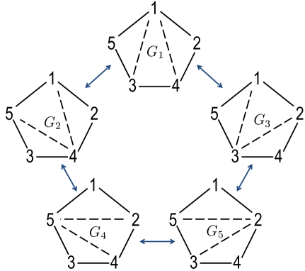
In this subsection, we will discuss the flip invariance of the decagon, i.e. we are going to show that the contribution of the mirror particles is independent of the way one decomposes the decagon into hexagons. The decagon which is a polygon with both five physical and five mirror edges appears for example in the computation of the five-point function of length two BPS operators. As discussed before, we are considering a restricted kinematics where all five operators are in a plane (we also impose an analogous constraint on the R-charge polarizations). The configuration is characterized by the set of cross ratios given in (LABEL:eq:TheCrossRatios).
Refer to caption
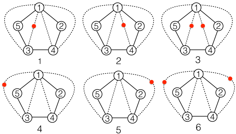
Figure 7: The flip invariance of the decagon. Each diagram in the figure corresponds to a different way of cutting the decagon into hexagons. They all give the same answer.

At one loop level, we have two one-particle contributions coming from each zero-length bridge and a two-particle contribution, which represents the interaction between two one-particle states (see figure 2). Depending on how we cut the decagon into three hexagons, we obtain the following expressions121212Here, for simplicity, we did not write the R𝑅R-charge cross-ratio argument of (1)superscript1\mathcal{M}^{(1)} and (2)superscript2\mathcal{M}^{(2)}. :

G1subscript𝐺1\displaystyle G_{1} =(1)(z)+(1)(1w1)+(2)(z,1w1),absentsuperscript1𝑧superscript11superscript𝑤1superscript2𝑧1superscript𝑤1\displaystyle=\mathcal{M}^{(1)}\left(z\right)+\mathcal{M}^{(1)}\left(1-w^{-1}\right)+\mathcal{M}^{(2)}\left(z,1-w^{-1}\right)\,, (43)
G2subscript𝐺2\displaystyle G_{2} =(1)(11w1)+(1)(zw)+(2)(11w1,zw),absentsuperscript111superscript𝑤1superscript1𝑧𝑤superscript211superscript𝑤1𝑧𝑤\displaystyle=\mathcal{M}^{(1)}\left(\frac{1}{1-w^{-1}}\right)+\mathcal{M}^{(1)}\left(\frac{z}{w}\right)+\mathcal{M}^{(2)}\left(\frac{1}{1-w^{-1}},\frac{z}{w}\right)\,,
G3subscript𝐺3\displaystyle G_{3} =(1)(1w11z1)+(1)(1z)+(2)(1w11z1,1z),absentsuperscript11superscript𝑤11superscript𝑧1superscript11𝑧superscript21superscript𝑤11superscript𝑧11𝑧\displaystyle=\mathcal{M}^{(1)}\left(\frac{1-w^{-1}}{1-z^{-1}}\right)+\mathcal{M}^{(1)}\left(\frac{1}{z}\right)+\mathcal{M}^{(2)}\left(\frac{1-w^{-1}}{1-z^{-1}},\frac{1}{z}\right)\,,
G4subscript𝐺4\displaystyle G_{4} =(1)(wz)+(1)(wzw1)+(2)(wz,wzw1),absentsuperscript1𝑤𝑧superscript1𝑤𝑧𝑤1superscript2𝑤𝑧𝑤𝑧𝑤1\displaystyle=\mathcal{M}^{(1)}\left(\frac{w}{z}\right)+\mathcal{M}^{(1)}\left(\frac{w-z}{w-1}\right)+\mathcal{M}^{(2)}\left(\frac{w}{z},\frac{w-z}{w-1}\right)\,,
G5subscript𝐺5\displaystyle G_{5} =(1)(w1wz)+(1)(1z11w1)+(2)(w1wz,1z11w1).absentsuperscript1𝑤1𝑤𝑧superscript11superscript𝑧11superscript𝑤1superscript2𝑤1𝑤𝑧1superscript𝑧11superscript𝑤1\displaystyle=\mathcal{M}^{(1)}\left(\frac{w-1}{w-z}\right)+\mathcal{M}^{(1)}\left(\frac{1-z^{-1}}{1-w^{-1}}\right)+\mathcal{M}^{(2)}\left(\frac{w-1}{w-z},\frac{1-z^{-1}}{1-w^{-1}}\right)\,.

Here Gisubscript𝐺𝑖G_{i} denotes the expression coming from each configuration in figure 7. Using the expressions for (1)superscript1\mathcal{M}^{(1)} and (2)superscript2\mathcal{M}^{(2)} given in (6) and (11), one can show that all the Gisubscript𝐺𝑖G_{i} above are equal. This establishes the flip invariance of the decagon.

4 Next-to-Extremal Four-Point Functions

In [5], it was conjectured that one only needs to compute the mirror-particle corrections associated with 1-edge irreducible (1EI) graphs in order to reproduce the correlation functions of BPS operators. This is equivalent to saying that the mirror-particle corrections associated with a non-1EI graph cancel among themselves131313 Recently in [11], an interesting proposal was made regarding the non-1EI graphs. They proposed that one should multiply the color factors to each hexagons and attributed the cancellation of the non-1EI graphs to such color factors. Nicely as we show here, the color factors do not seem necessary to observe the cancellation. This and related issues will be discussed more in detail in [9, 10]. . Due to the fact that non-1EI graphs have multiple length-zero bridges, showing the cancellation requires the knowledge of the multi-particle contribution. In this section, using the two-particle contribution computed in the previous section, we show this cancellation explicitly for the so-called next-to-extremal four-point functions at one loop. To show it for more general one-loop four-point functions, one needs three-particle contributions and we will leave it for future investigations.

Let us consider the four-point function of three length-two BPS operators and one length-four BPS operator which we choose to be the operator four. This is an example of a next-to-extremal correlator because the lengths satisfy the defining condition L4=L1+L2+L32subscript𝐿4subscript𝐿1subscript𝐿2subscript𝐿32L_{4}=L_{1}+L_{2}+L_{3}-2. This kind of correlators is known to be protected [13, 12, 14]. Namely the quantum corrections to this correlator must vanish.

Refer to caption
Figure 8: An example of the tree-level Wick contraction for G{2,2,2,4}subscript𝐺2224G_{\{2,2,2,4\}} and its mirror-particle corrections. Other diagrams, which are also non-1EI, can be obtained by permuting the indices of the length-222 operators. The sum of the contributions depicted above vanishes in agreement with the non-renormalization property of the next-to-extremal correlator.

From the hexagonalization point of view, the computation of this correlator only involves non-1EI graphs. An example of non-1EI graphs and its mirror-particle corrections at one loop are given in figure 8. The remaining ones can be obtained by permuting the indices of the external operators. Using the result in the previous section, one can compute it explicitly as

Figure8=d142d23d24d34[(1)(1z1,1α1)+(1)(11z,11α)\displaystyle{\rm{Figure}}\,\,\ref{fig:The2224}\;=\;d_{14}^{2}d_{23}d_{24}d_{34}\,\left[\,\mathcal{M}^{(1)}(1-z^{-1},1-\alpha^{-1})+\mathcal{M}^{(1)}\left(\frac{1}{1-z},\frac{1}{1-\alpha}\right)\right. (44)
+(2)(1z1,11z,1α1,11α)].\displaystyle\left.+\,\mathcal{M}^{(2)}\left(1-z^{-1},\frac{1}{1-z},1-\alpha^{-1},\frac{1}{1-\alpha}\right)\right]\,.

Using (13) and the properties of m(z)𝑚𝑧m(z) given in (10), one obtains

Figure8=d142d23d24d34[m(zz1)+m(11z)+2m(1)+m(0)]=0.Figure8superscriptsubscript𝑑142subscript𝑑23subscript𝑑24subscript𝑑34delimited-[]𝑚𝑧𝑧1𝑚11𝑧2𝑚1𝑚00{\rm{Figure}}\,\,\ref{fig:The2224}\;=d_{14}^{2}d_{23}d_{24}d_{34}\left[m\left(\frac{z}{z-1}\right)+m\left(\frac{1}{1-z}\right)+2m(1)+m(0)\right]=0\,. (45)

This proves the absence of one-loop corrections to this four-point function.
Refer to caption
Refer to caption
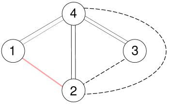
Figure 9: Examples of graphs for the extremal four-point functions. The solid black lines are the propagators while the red thick lines are the additional propagator one adds to make them into graphs for the next-to-extremal four-point functions. In the left figure, the resulting next-to-extremal graph contains two length-zero bridges (denoted by the dashed lines), while in the right figure, it only has one length-zero bridge whose cross ratio is unity.

Although we have focused on one particular example so far, the argument presented here can be readily applied to general next-to-extremal four-point functions. To see this, one just needs to use the fact that the graphs for the next-to-extremal four-point functions (satisfying L4=L1+L2+L32subscript𝐿4subscript𝐿1subscript𝐿2subscript𝐿32L_{4}=L_{1}+L_{2}+L_{3}-2) can be obtained by

  1. 1.

    First drawing the graphs for the extremal correlator GL11,L21,L3,L4subscript𝐺subscript𝐿11subscript𝐿21subscript𝐿3subscript𝐿4G_{L_{1}-1,L_{2}-1,L_{3},L_{4}}.

  2. 2.

    Then adding one propagator between 𝒪1subscript𝒪1\mathcal{O}_{1} and 𝒪2subscript𝒪2\mathcal{O}_{2}.

It is straightforward to see that the graphs for the extremal correlator contain three or two length-zero bridges. Thus, if we add one propagator as in step 2 above, we are left with graphs with two zero-length bridges or graphs with a single zero-length bridge (see figure 9). The graphs with two zero-length bridges have the same topology as the one in figure 8, and therefore the contributions from such a graph add up to zero. On the other hand, for the graphs with a single zero-length bridge, the cross ratios associated with the zero-length bridge are 111. By taking the limit z,z¯1𝑧¯𝑧1z,\bar{z}\to 1 and α,α¯1𝛼¯𝛼1\alpha,\bar{\alpha}\to 1 in the one-particle mirror contribution (6), one can show that the mirror-particle corrections to these graphs also vanish. Thus, in summary, the one-loop correction to the next-to-extremal four-point functions always vanishes, in agreement with the non-renormalization theorem shown in [14].

Note also that the cancellation proven in this section holds at the level of individual graphs. Therefore, one can use the result here to show that many of the non-1EI graphs (that appear in more general four-point functions) do not contribute at one loop. The only graphs that are not covered by the discussion here are the graphs which contain three length-zero bridges, such as the ones that appear in the extremal four-point functions. It would be an interesting future problem to compute the three-particle contributions and show the cancellation in full generality.

5 Summary and Possible Applications

In this paper, we have computed the two-particle mirror contribution at one loop. Using its result, we computed two five-point correlators using integrability and have found agreement with the perturbative data. In addition, we proved that the contributions from non-1EI graphs that appear in the next-to-extremal four-point functions add up to zero, thereby giving supports to the prescription in the previous paper [5] which states that one only needs to consider corrections from 1EI graphs.

In this paper, we only considered the five-point functions in a restricted kinematics where all the operators lie in a two-dimensional plane. It would be an interesting future direction to generalize the computation performed here to the five-point function in general kinematics. As already mentioned, to study the general kinematics, one needs to include in the weight factors the generators that take the operators away from the plane. As a consequence, the non-diagonal elements of the mirror S𝑆S-matrix (computed in Appendix B) will also show up in the computation. Although this makes the computation slightly more involved, there is no additional conceptual difficulty in doing this.

The techniques developed in this paper, in particular the Z𝑍Z-marker dressing and the calculation of the mirror bound state S𝑆S-matrix can be used to evaluate the higher-particle contributions which are necessary for computing the higher-loop corrections and the non-planar correlators. In particular, it is interesting to compute the two-(and three-)loop four-point functions and see if one can reproduce the perturbative data [15].

Another interesting application would be to use the hexagonalization to evaluate complicated Feynman integrals. Recently in [16], they succeeded in evaluating particular sets of fishnet diagrams, which generalize the conformal ladder integrals, by using the hexagonalization (and also by the pentagon OPE). It would be interesting to try to extract other integrals that have not yet been computed, such as the double box integrals, by using the two- and higher-particle contributions. For this purpose, it would perhaps be useful to apply the hexagonalization approach to the strongly deformed planar 𝒩=4𝒩4\mathcal{N}=4 SYM proposed recently [17, 18, 19, 20, 21, 22] since many quantities in this theory admit only a single Feynman diagram at each loop order, and it should be easier to identify the contribution from a given Feynman graph.

Acknowledgements

We acknowledge discussions with and comments by B. Basso, T. Bargheer, J. Caetano, V. Goncalves, V. Kazakov, G. Korchemsky. Especially, we thank P. Vieira for helping us with the evaluation of the integral, in particular by suggesting the basis of functions used. T. F. would like to thank the warm hospitality of the Perimeter Institute and of the Laboratoire de Physique Théorique de l’Ecole Normale Supérieure were a large part of this work was done. T. F. would like to thank CAPES/INCTMAT process 88887.143256/2017-00, the Perimeter Institute and the European Research Council (Programme ERC-2012- AdG 320769 AdS-CFT-solvable) for financial support. S.K. is supported by the US Department of Energy.

Appendix A The Z𝑍Z-marker Dressing

As discussed in [5], the naive basis for the mirror bound states does not reproduce the perturbative data and it is necessary to dress it with Z𝑍Z-markers. In this section, we explain how to dress the two-particle states by Z𝑍Z-markers141414At the moment, we do not have a clear-cut physical explanation for the prescription. However, adding the Z𝑍Z-markers removes all the unwanted square-root cuts of the integrand and makes all the states of the bound-state multiplet produce a non-zero contribution to the integral. This means that it should be somehow related to the supersymmetry. .

A.1 Review of Z𝑍Z-marker dressing for one-particle states

Let us first briefly review the rule to dress the one-particle states. The a𝑎a-th bound state 𝒳𝒳\mathcal{X} is made up of a pair of “quarks” χ𝜒\chi and χ˙˙𝜒\dot{\chi}, each of which belongs to the a𝑎a-th anti-symmetric representation of 𝔭𝔰𝔲(2|2)𝔭𝔰𝔲conditional22\mathfrak{psu}(2|2):

χ,χ˙=𝜒˙𝜒absent\displaystyle\chi\,,\,\,\dot{\chi}= |ψα1ψαa+,ketsubscript𝜓subscript𝛼1subscript𝜓subscript𝛼𝑎\displaystyle|\psi_{\alpha_{1}}\cdots\psi_{\alpha_{a}}\rangle+\cdots\,,\quad |ϕ1ψa1ψαa1+,ketsubscriptitalic-ϕ1subscript𝜓subscript𝑎1subscript𝜓subscript𝛼𝑎1\displaystyle|\phi_{1}\psi_{a_{1}}\cdots\psi_{\alpha_{a-1}}\rangle+\cdots\,, (46)
|ϕ2ψα1ψαa1+,ketsubscriptitalic-ϕ2subscript𝜓subscript𝛼1subscript𝜓subscript𝛼𝑎1\displaystyle|\phi_{2}\psi_{\alpha_{1}}\cdots\psi_{\alpha_{a-1}}\rangle+\cdots\,,\quad |ϕ1ϕ2ψα1ψαa2+,ketsubscriptitalic-ϕ1subscriptitalic-ϕ2subscript𝜓subscript𝛼1subscript𝜓subscript𝛼𝑎2\displaystyle|\phi_{1}\phi_{2}\psi_{\alpha_{1}}\cdots\psi_{\alpha_{a-2}}\rangle+\cdots\,,

To correctly reproduce the four-point function perturbative data, one must dress the states containing bosons ϕ1subscriptitalic-ϕ1\phi_{1} and ϕ2subscriptitalic-ϕ2\phi_{2} (and their dotted counter parts) as follows:

+ dressing::+ dressingabsent\displaystyle\text{$+$ dressing}: ϕ1Z12ϕ1,ϕ2Z12ϕ2,ϕ˙1Z12ϕ˙1,ϕ˙2Z12ϕ˙2,formulae-sequencesubscriptitalic-ϕ1superscript𝑍12subscriptitalic-ϕ1formulae-sequencesubscriptitalic-ϕ2superscript𝑍12subscriptitalic-ϕ2formulae-sequencesubscript˙italic-ϕ1superscript𝑍12subscript˙italic-ϕ1subscript˙italic-ϕ2superscript𝑍12subscript˙italic-ϕ2\displaystyle\phi_{1}\to Z^{\frac{1}{2}}\,\phi_{1}\,,\quad\phi_{2}\to Z^{-\frac{1}{2}}\,\phi_{2}\,,\quad\dot{\phi}_{1}\to Z^{-\frac{1}{2}}\,\dot{\phi}_{1}\,,\quad\dot{\phi}_{2}\to Z^{\frac{1}{2}}\,\dot{\phi}_{2}\,, (47)
 dressing:: dressingabsent\displaystyle\text{$-$ dressing}: ϕ1Z12ϕ1,ϕ2Z12ϕ2,ϕ˙1Z12ϕ˙1,ϕ˙2Z12ϕ˙2.formulae-sequencesubscriptitalic-ϕ1superscript𝑍12subscriptitalic-ϕ1formulae-sequencesubscriptitalic-ϕ2superscript𝑍12subscriptitalic-ϕ2formulae-sequencesubscript˙italic-ϕ1superscript𝑍12subscript˙italic-ϕ1subscript˙italic-ϕ2superscript𝑍12subscript˙italic-ϕ2\displaystyle\phi_{1}\to Z^{-\frac{1}{2}}\,\phi_{1}\,,\quad\phi_{2}\to Z^{\frac{1}{2}}\,\phi_{2}\,,\quad\dot{\phi}_{1}\to Z^{\frac{1}{2}}\,\dot{\phi}_{1}\,,\quad\dot{\phi}_{2}\to Z^{-\frac{1}{2}}\dot{\phi}_{2}\,.

and average over ++ and - dressings at the end of the computation. (Note that the dressings for the left 𝔭𝔰𝔲(2|2)𝔭𝔰𝔲conditional22\mathfrak{psu}(2|2) and the right 𝔭𝔰𝔲(2|2)𝔭𝔰𝔲conditional22\mathfrak{psu}(2|2) are different). For instance, for the fundamental magnons, we dress the states in the following way:

+ dressing::+ dressingabsent\displaystyle\text{$+$ dressing}: (48)
Dαα˙Dαα˙,Φ12ZΦ12,Φ21Z1Φ21,Φ11Φ11,Φ22Φ22,formulae-sequencesubscript𝐷𝛼˙𝛼subscript𝐷𝛼˙𝛼formulae-sequencesubscriptΦ12𝑍subscriptΦ12formulae-sequencesubscriptΦ21superscript𝑍1subscriptΦ21formulae-sequencesubscriptΦ11subscriptΦ11subscriptΦ22subscriptΦ22\displaystyle\quad D_{\alpha\dot{\alpha}}\to D_{\alpha\dot{\alpha}}\,,\quad\Phi_{12}\to Z\,\Phi_{12}\,,\quad\Phi_{21}\to Z^{-1}\,\Phi_{21}\,,\quad\Phi_{11}\to\Phi_{11}\,,\quad\Phi_{22}\to\Phi_{22}\,,
Ψ1α˙Z12Ψ1α˙,Ψ2α˙Z12Ψ2α˙,Ψα1˙Z12Ψα1˙,Ψα2˙Z12Ψα2˙.formulae-sequencesubscriptΨ1˙𝛼superscript𝑍12subscriptΨ1˙𝛼formulae-sequencesubscriptΨ2˙𝛼superscript𝑍12subscriptΨ2˙𝛼formulae-sequencesubscriptΨ𝛼˙1superscript𝑍12subscriptΨ𝛼˙1subscriptΨ𝛼˙2superscript𝑍12subscriptΨ𝛼˙2\displaystyle\quad\Psi_{1\dot{\alpha}}\to Z^{\frac{1}{2}}\,\Psi_{1\dot{\alpha}}\,,\quad\Psi_{2\dot{\alpha}}\to Z^{-\frac{1}{2}}\,\Psi_{2\dot{\alpha}}\,,\quad\Psi_{\alpha\dot{1}}\to Z^{-\frac{1}{2}}\,\Psi_{\alpha\dot{1}}\,,\quad\Psi_{\alpha\dot{2}}\to Z^{\frac{1}{2}}\,\Psi_{\alpha\dot{2}}\,.
 dressing:: dressingabsent\displaystyle\text{$-$ dressing}:
Dαα˙Dαα˙,Φ12Z1Φ12,Φ21ZΦ21,Φ11Φ11,Φ22Φ22,formulae-sequencesubscript𝐷𝛼˙𝛼subscript𝐷𝛼˙𝛼formulae-sequencesubscriptΦ12superscript𝑍1subscriptΦ12formulae-sequencesubscriptΦ21𝑍subscriptΦ21formulae-sequencesubscriptΦ11subscriptΦ11subscriptΦ22subscriptΦ22\displaystyle\quad D_{\alpha\dot{\alpha}}\to D_{\alpha\dot{\alpha}}\,,\quad\Phi_{12}\to Z^{-1}\,\Phi_{12}\,,\quad\Phi_{21}\to Z\,\Phi_{21}\,,\quad\Phi_{11}\to\Phi_{11}\,,\quad\Phi_{22}\to\Phi_{22}\,,
Ψ1α˙Z12Ψ1α˙,Ψ2α˙Z12Ψ2α˙,Ψα1Z12Ψα1,Ψα2Z12Ψα2.formulae-sequencesubscriptΨ1˙𝛼superscript𝑍12subscriptΨ1˙𝛼formulae-sequencesubscriptΨ2˙𝛼superscript𝑍12subscriptΨ2˙𝛼formulae-sequencesubscriptΨ𝛼1superscript𝑍12subscriptΨ𝛼1subscriptΨ𝛼2superscript𝑍12subscriptΨ𝛼2\displaystyle\quad\Psi_{1\dot{\alpha}}\to Z^{-\frac{1}{2}}\,\Psi_{1\dot{\alpha}}\,,\quad\Psi_{2\dot{\alpha}}\to Z^{\frac{1}{2}}\,\Psi_{2\dot{\alpha}}\,,\quad\Psi_{\alpha 1}\to Z^{\frac{1}{2}}\,\Psi_{\alpha 1}\,,\quad\Psi_{\alpha 2}\to Z^{-\frac{1}{2}}\,\Psi_{\alpha 2}\,.
Refer to caption
Figure 10: The configuration of mirror particles which produces the one-particle contribution. One can glue the edge 141414 by either putting a virtual-particle pair on the edge 111.

Let us also recall how the weight factors are affected by the Z-marker dressings. In what follows, we only discuss the fundamental magnon, but the generalization to the bound states is straightforward. To figure out the effect of the dressing, it is useful to think of the gluing as the process of putting virtual particle pairs in the adjacent physical edges and making the edges entangled [5]. (See also figure 10). Let us consider the configuration depicted in figure 10, and try to glue the mirror edge 141414 by putting a virtual particle pair on the edge 111. In this case, the particle pairs are dressed in the following way:

|Zt𝒳(±)𝒳¯(uγ)left hexagon|𝒳(uγ)Z+t𝒳(±)right hexagon.tensor-productsubscriptketsuperscript𝑍superscriptsubscript𝑡𝒳plus-or-minus¯𝒳superscript𝑢𝛾left hexagonsubscriptket𝒳superscript𝑢𝛾superscript𝑍superscriptsubscript𝑡𝒳plus-or-minusright hexagon\displaystyle\underbrace{|Z^{-t_{\mathcal{X}}^{(\pm)}}\bar{\mathcal{X}}(u^{-\gamma})\rangle}_{\text{left hexagon}}\otimes\underbrace{|\mathcal{X}(u^{\gamma})Z^{+t_{\mathcal{X}}^{(\pm)}}\rangle}_{\text{right hexagon}}\,. (49)

Here the superscript (±)plus-or-minus(\pm) in t𝒳(±)superscriptsubscript𝑡𝒳plus-or-minust_{\mathcal{X}}^{(\pm)} denotes the choice of the ++ or the - dressing and t𝒳(+)(=t𝒳())annotatedsuperscriptsubscript𝑡𝒳absentsuperscriptsubscript𝑡𝒳t_{\mathcal{X}}^{(+)}(=-t_{\mathcal{X}}^{(-)}) is determined from (48) as

tDαα˙(+)=0,tΦ12(+)=1,tΦ21(+)=1,tΦ11(+)=tΦ22(+)=0,formulae-sequencesuperscriptsubscript𝑡subscript𝐷𝛼˙𝛼0formulae-sequencesuperscriptsubscript𝑡subscriptΦ121formulae-sequencesuperscriptsubscript𝑡subscriptΦ211superscriptsubscript𝑡subscriptΦ11superscriptsubscript𝑡subscriptΦ220\displaystyle\quad t_{D_{\alpha\dot{\alpha}}}^{(+)}=0\,,\quad t_{\Phi_{12}}^{(+)}=1\,,\quad t_{\Phi_{21}}^{(+)}=-1\,,\quad t_{\Phi_{11}}^{(+)}=t_{\Phi_{22}}^{(+)}=0\,, (50)
tΨ1α˙(+)=tΨα2˙(+)=1/2,tΨ2α˙(+)=tΨα1˙(+)=1/2.formulae-sequencesuperscriptsubscript𝑡subscriptΨ1˙𝛼superscriptsubscript𝑡subscriptΨ𝛼˙212superscriptsubscript𝑡subscriptΨ2˙𝛼superscriptsubscript𝑡subscriptΨ𝛼˙112\displaystyle\quad t_{\Psi_{1\dot{\alpha}}}^{(+)}=t_{\Psi_{\alpha\dot{2}}}^{(+)}=1/2\,,\quad t_{\Psi_{2\dot{\alpha}}}^{(+)}=t_{\Psi_{\alpha\dot{1}}}^{(+)}=-1/2\,.

Comparing (50) with table 1, one can see that t𝒳(+)superscriptsubscript𝑡𝒳t_{\mathcal{X}}^{(+)} coincides with the eigenvalues of the R-symmetry rotation generator

R=12(R11R22R1˙+1˙R2˙)2˙.R=\frac{1}{2}(R^{1}{}_{1}-R^{2}{}_{2}-R^{\dot{1}}{}_{\dot{1}}+R^{\dot{2}}{}_{\dot{2}})\,. (51)

Therefore, one can express the flavor-dependent weight factor as

𝒲flavor=eiJ𝒳φeiL𝒳ϕeiR𝒳θ=eiL𝒳ϕeiR𝒳(θ±φ),subscript𝒲flavorsuperscript𝑒𝑖subscript𝐽𝒳𝜑superscript𝑒𝑖subscript𝐿𝒳italic-ϕsuperscript𝑒𝑖subscript𝑅𝒳𝜃superscript𝑒𝑖subscript𝐿𝒳italic-ϕsuperscript𝑒𝑖subscript𝑅𝒳plus-or-minus𝜃𝜑\mathcal{W}_{{\rm{flavor}}}=e^{iJ_{\mathcal{X}}\varphi}\,e^{iL_{\mathcal{X}}\phi}\,e^{iR_{\mathcal{X}}\theta}=e^{iL_{\mathcal{X}}\phi}\,e^{iR_{\mathcal{X}}(\theta\pm\varphi)}\,, (52)

where ±plus-or-minus\pm correspond to the ++ and - dressings respectively. In sum, the net effect of the Z𝑍Z-marker dressing for the one-particle state is to change θ𝜃\theta to θ+φ𝜃𝜑\theta+\varphi or θφ𝜃𝜑\theta-\varphi depending on the choice of the dressings.

A.2 Z𝑍Z-marker dressing for two-particle states
Refer to caption
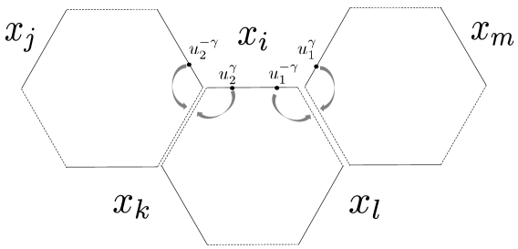
Figure 11: The configuration of the mirror particles which produces the two-particle contribution.

We now explain how to dress the two-particles states (one particle for each edge, see figure 11). For simplicity, we again consider fundamental magnons only.

The prescription for the two-particle states is a natural generalization of the one for the one-particle states. Namely we propose to dress the state in the following way,

|Zt𝒳2(±)𝒳¯2(u2γ)left hexagon|𝒳2(u2γ)Z+t𝒳2(±)Zt𝒳1(±)𝒳¯1(u1γ)middle hexagon|𝒳1(u1γ)Z+t𝒳1(±)right hexagon.tensor-productsubscriptketsuperscript𝑍superscriptsubscript𝑡subscript𝒳2plus-or-minussubscript¯𝒳2superscriptsubscript𝑢2𝛾left hexagonsubscriptketsubscript𝒳2superscriptsubscript𝑢2𝛾superscript𝑍superscriptsubscript𝑡subscript𝒳2plus-or-minussuperscript𝑍superscriptsubscript𝑡subscript𝒳1plus-or-minussubscript¯𝒳1superscriptsubscript𝑢1𝛾middle hexagonsubscriptketsubscript𝒳1superscriptsubscript𝑢1𝛾superscript𝑍superscriptsubscript𝑡subscript𝒳1plus-or-minusright hexagon\underbrace{|Z^{-t_{\mathcal{X}_{2}}^{(\pm)}}\bar{\mathcal{X}}_{2}(u_{2}^{-\gamma})\rangle}_{\text{left hexagon}}\otimes\underbrace{|\mathcal{X}_{2}(u_{2}^{\gamma})Z^{+t_{\mathcal{X}_{2}}^{(\pm)}}Z^{-t_{\mathcal{X}_{1}}^{(\pm)}}\bar{\mathcal{X}}_{1}(u_{1}^{-\gamma})\rangle}_{\text{middle hexagon}}\otimes\underbrace{|\mathcal{X}_{1}(u_{1}^{\gamma})Z^{+t_{\mathcal{X}_{1}}^{(\pm)}}\rangle}_{\text{right hexagon}}\,. (53)

and average over the two choices, (±)plus-or-minus(\pm). (Note that we do not sum over 2×2=42242\times 2=4 choices of the signs: The choices of the signs in t𝒳1subscript𝑡subscript𝒳1t_{\mathcal{X}_{1}} and t𝒳2subscript𝑡subscript𝒳2t_{\mathcal{X}_{2}} must be correlated.) For the two-particle state, the effect of the Z𝑍Z-markers is twofold: One is to introduce the J𝐽J-charge and change the flavor dependent weight factor. As in the one-particle case, the net effect is to change θisubscript𝜃𝑖\theta_{i} to θi±φiplus-or-minussubscript𝜃𝑖subscript𝜑𝑖\theta_{i}\pm\varphi_{i}. (θisubscript𝜃𝑖\theta_{i} and φisubscript𝜑𝑖\varphi_{i} are the angles for the two channels.) The other is the phase shift induced by moving and removing the Z𝑍Z-markers in the state (53). Using the rule given in [6], one obtains

eit𝒳1(±)p(u2γ)/2+it𝒳2(±)p(u1γ)/2|𝒳¯2(u2γ)|𝒳2(u2γ)𝒳¯1(u1γ)|𝒳1(u1γ).tensor-productsuperscript𝑒𝑖superscriptsubscript𝑡subscript𝒳1plus-or-minus𝑝superscriptsubscript𝑢2𝛾2𝑖superscriptsubscript𝑡subscript𝒳2plus-or-minus𝑝superscriptsubscript𝑢1𝛾2ketsubscript¯𝒳2superscriptsubscript𝑢2𝛾ketsubscript𝒳2superscriptsubscript𝑢2𝛾subscript¯𝒳1superscriptsubscript𝑢1𝛾ketsubscript𝒳1superscriptsubscript𝑢1𝛾e^{-it_{\mathcal{X}_{1}}^{(\pm)}p(u_{2}^{\gamma})/2+it_{\mathcal{X}_{2}}^{(\pm)}p(u_{1}^{\gamma})/2}|\bar{\mathcal{X}}_{2}(u_{2}^{-\gamma})\rangle\otimes|\mathcal{X}_{2}(u_{2}^{\gamma})\bar{\mathcal{X}}_{1}(u_{1}^{-\gamma})\rangle\otimes|\mathcal{X}_{1}(u_{1}^{\gamma})\rangle\,. (54)

Using the fact that t𝒳(+)superscriptsubscript𝑡𝒳t_{\mathcal{X}}^{(+)} coincides with the eigenvalue of the R𝑅R generator, we arrive at the following effective replacement rule, which implements the Z𝑍Z-marker dressing:

+ dressing::+ dressingabsent\displaystyle\text{$+$ dressing}: θ1θ1+φ1p(u2γ)/2,θ2θ2+φ2+p(u1γ)/2,formulae-sequencesubscript𝜃1subscript𝜃1subscript𝜑1𝑝superscriptsubscript𝑢2𝛾2subscript𝜃2subscript𝜃2subscript𝜑2𝑝superscriptsubscript𝑢1𝛾2\displaystyle\quad\theta_{1}\to\theta_{1}+\varphi_{1}-p(u_{2}^{\gamma})/2\,,\qquad\theta_{2}\to\theta_{2}+\varphi_{2}+p(u_{1}^{\gamma})/2\,, (55)
 dressing:: dressingabsent\displaystyle\text{$-$ dressing}: θ1θ1φ1+p(u2γ)/2,θ2θ2φ2p(u1γ)/2.formulae-sequencesubscript𝜃1subscript𝜃1subscript𝜑1𝑝superscriptsubscript𝑢2𝛾2subscript𝜃2subscript𝜃2subscript𝜑2𝑝superscriptsubscript𝑢1𝛾2\displaystyle\quad\theta_{1}\to\theta_{1}-\varphi_{1}+p(u_{2}^{\gamma})/2\,,\qquad\theta_{2}\to\theta_{2}-\varphi_{2}-p(u_{1}^{\gamma})/2\,.

Written more explicitly, the additional phases for scalars in the ++ dressing are given as follows:

𝒳1(u1γ)::subscript𝒳1superscriptsubscript𝑢1𝛾absent\displaystyle\mathcal{X}_{1}(u_{1}^{\gamma}): Φ12(u1γ)ei(θ1+φ1p(u2γ)/2),subscriptΦ12superscriptsubscript𝑢1𝛾superscript𝑒𝑖subscript𝜃1subscript𝜑1𝑝superscriptsubscript𝑢2𝛾2\displaystyle\quad\Phi_{12}(u_{1}^{\gamma})\to e^{i(\theta_{1}+\varphi_{1}-p(u_{2}^{\gamma})/2)}\,,\qquad Φ21(u1γ)ei(θ1+φ1p(u2γ)/2),subscriptΦ21superscriptsubscript𝑢1𝛾superscript𝑒𝑖subscript𝜃1subscript𝜑1𝑝superscriptsubscript𝑢2𝛾2\displaystyle\Phi_{21}(u_{1}^{\gamma})\to e^{-i(\theta_{1}+\varphi_{1}-p(u_{2}^{\gamma})/2)}\,, (56)
𝒳2(u2γ)::subscript𝒳2superscriptsubscript𝑢2𝛾absent\displaystyle\mathcal{X}_{2}(u_{2}^{\gamma}): Φ12(u2γ)ei(θ2+φ2+p(u1γ)/2),subscriptΦ12superscriptsubscript𝑢2𝛾superscript𝑒𝑖subscript𝜃2subscript𝜑2𝑝superscriptsubscript𝑢1𝛾2\displaystyle\quad\Phi_{12}(u_{2}^{\gamma})\to e^{i(\theta_{2}+\varphi_{2}+p(u_{1}^{\gamma})/2)}\,,\qquad Φ21(u2γ)ei(θ2+φ2+p(u1γ)/2).subscriptΦ21superscriptsubscript𝑢2𝛾superscript𝑒𝑖subscript𝜃2subscript𝜑2𝑝superscriptsubscript𝑢1𝛾2\displaystyle\Phi_{21}(u_{2}^{\gamma})\to e^{-i(\theta_{2}+\varphi_{2}+p(u_{1}^{\gamma})/2)}\,.

As mentioned in the main text, it is convenient for the actual computation to perform the mirror transformation to the middle hexagon and rewrite it as

|𝒳2(u2γ)𝒳¯1(u1γ)|𝒳1(u15γ)𝒳2(u2γ).maps-toketsubscript𝒳2superscriptsubscript𝑢2𝛾subscript¯𝒳1superscriptsubscript𝑢1𝛾ketsubscript𝒳1superscriptsubscript𝑢15𝛾subscript𝒳2superscriptsubscript𝑢2𝛾|\mathcal{X}_{2}(u_{2}^{\gamma})\bar{\mathcal{X}}_{1}(u_{1}^{-\gamma})\rangle\mapsto|\mathcal{X}_{1}(u_{1}^{5\gamma})\mathcal{X}_{2}(u_{2}^{\gamma})\rangle\,. (57)

After this rewriting, one can read off the flavor-dependent weight factors just by looking at the charges of what are inside the middle hexagon151515Originally the middle hexagon contained 𝒳¯1subscript¯𝒳1\bar{\mathcal{X}}_{1} and we needed to invert the charge to read off the correct weight factor..

The prescription for the Z𝑍Z-marker dressing we described here can be straightforwardly generalized to the multi-particle states. It is an interesting future problem to perform the multi-particle computation explicitly and see if the prescription reproduces the correct answer. Also important is to understand the origin of this Z𝑍Z-marker prescription. From various circumstantial evidence, we know that it must be related to how the supersymmetry is realized in the hexagon formalism, but it would be nice if we can make it more precise. It would also be desirable to understand it from the viewpoint of the string worldsheet theory161616The necessity of the discrete sum is a bit reminiscent of the sum over the spin structure although it cannot be the same thing..

Appendix B The Bound State-Bound State Mirror S-matrix

The matrix part of the hexagon form factor needed to evaluate the two-particle contribution is given by the elements of the mirror bound state S𝑆S-matrix. The physical bound state S𝑆S-matrix was computed in [23] using its Yangian invariance. In order to compute the necessary mirror bound state S𝑆S-matrix, we only need to adapt the procedure described in [23] to our case.

B.1 Basis and Invariant Subsectors

In our case, the bound state with index a𝑎a is in the a𝑎a-th anti-symmetric representation of 𝔰𝔲(2|2)𝔰𝔲conditional22\mathfrak{su}(2|2). A basis is given by

|ψα1ψαa+,ketsubscript𝜓subscript𝛼1subscript𝜓subscript𝛼𝑎\displaystyle|\psi_{\alpha_{1}}\cdots\psi_{\alpha_{a}}\rangle+\ldots\,,\quad\;\;\; |ϕ1ψα1ψαa1+,ketsubscriptitalic-ϕ1subscript𝜓subscript𝛼1subscript𝜓subscript𝛼𝑎1\displaystyle\quad\quad\quad|\phi_{1}\psi_{\alpha_{1}}\cdots\psi_{\alpha_{a-1}}\rangle+\ldots\,,
|ϕ2ψα1ψαa1+,ketsubscriptitalic-ϕ2subscript𝜓subscript𝛼1subscript𝜓subscript𝛼𝑎1\displaystyle|\phi_{2}\psi_{\alpha_{1}}\cdots\psi_{\alpha_{a-1}}\rangle+\ldots\,, |ϕ1ϕ2ψα1ψαa2+.ketsubscriptitalic-ϕ1subscriptitalic-ϕ2subscript𝜓subscript𝛼1subscript𝜓subscript𝛼𝑎2\displaystyle\quad\quad\quad|\phi_{1}\phi_{2}\psi_{\alpha_{1}}\cdots\psi_{\alpha_{a-2}}\rangle+\ldots\,.

The S𝑆S-matrix is an operator acting in the tensor product of two bound states with indices a𝑎a and b𝑏b and rapidities u1subscript𝑢1u_{1} and u2subscript𝑢2u_{2} respectively. After the action of the S𝑆S-matrix the two spaces are interchanged, i.e.

S|u1,ai|u2,bj=(Sab)ijkl(u1,u2)|u2,bk|u1,al,tensor-product𝑆subscriptketsubscript𝑢1𝑎𝑖subscriptketsubscript𝑢2𝑏𝑗tensor-productsuperscriptsubscriptsubscript𝑆𝑎𝑏𝑖𝑗𝑘𝑙subscript𝑢1subscript𝑢2subscriptketsubscript𝑢2𝑏𝑘subscriptketsubscript𝑢1𝑎𝑙S\cdot\,|{u_{1},a}\rangle_{i}\otimes|{u_{2},b}\rangle_{j}=(S_{ab})_{ij}^{kl}(u_{1},u_{2})\,|{u_{2},b}\rangle_{k}\otimes|{u_{1},a}\rangle_{l}\,, (58)

where i,j,k𝑖𝑗𝑘i,j,k and l𝑙l denote the basis elements.

As discuted in [23] for the physical bound state S𝑆S-matrix and following the same reasoning, it is possible to show that the mirror bound state S𝑆S-matrix has a block diagonal structure. The S𝑆S-matrix commutes with 𝔰𝔲(2|2)𝔰𝔲conditional22\mathfrak{su}(2|2) and the generators of the algebra are the Lorentz rotations Lβα,subscriptsuperscript𝐿𝛼𝛽L^{\alpha}_{\;\;\beta}, the R𝑅R-charge rotations Rba,subscriptsuperscript𝑅𝑎𝑏R^{a}_{\;\;b}, and the supersymmetry generators Qaαsubscriptsuperscript𝑄𝛼𝑎Q^{\alpha}_{\;\;a} and Sαasubscriptsuperscript𝑆𝑎𝛼S^{a}_{\;\;\alpha}. In particular, the commutator of R  11subscriptsuperscript𝑅11R^{1}_{\;\;1} with the S𝑆S-matrix implies that the following quantity is conserved

C1=ϕ1iϕ2i+ϕ1jϕ2j,subscript𝐶1superscriptsubscriptitalic-ϕ1𝑖superscriptsubscriptitalic-ϕ2𝑖superscriptsubscriptitalic-ϕ1𝑗superscriptsubscriptitalic-ϕ2𝑗C_{1}=\sharp\,\phi_{1}^{i}-\sharp\,\phi_{2}^{i}+\sharp\,\phi_{1}^{j}-\sharp\,\phi_{2}^{j}\,, (59)

where the superscripts i𝑖i and j𝑗j refer to the first and to the second bound state being scattered and \sharp means the number of the corresponding fields. As a consequence of the form of the basis elements, the charge C1subscript𝐶1C_{1} can take the values C1=2,1,0,1,2subscript𝐶121012C_{1}=-2,-1,0,1,2 and one can use it to classify the following invariant subspaces under the action of the S𝑆S-matrix:

Case I

  • C1=2subscript𝐶12C_{1}=2:

    |k,lIa=|ϕ1ψ1ak1ψ2k|ϕ1ψ1bl1ψ2l.superscriptket𝑘𝑙Iatensor-productketsubscriptitalic-ϕ1superscriptsubscript𝜓1𝑎𝑘1superscriptsubscript𝜓2𝑘ketsubscriptitalic-ϕ1superscriptsubscript𝜓1𝑏𝑙1superscriptsubscript𝜓2𝑙\displaystyle|k,l\rangle^{{\rm{Ia}}}=|\phi_{1}\psi_{1}^{a-k-1}\psi_{2}^{k}\rangle\otimes|\phi_{1}\psi_{1}^{b-l-1}\psi_{2}^{l}\rangle\,.
  • C1=2subscript𝐶12C_{1}=-2:

    |k,lIb=|ϕ2ψ1ak1ψ2k|ϕ2ψ1bl1ψ2l.superscriptket𝑘𝑙Ibtensor-productketsubscriptitalic-ϕ2superscriptsubscript𝜓1𝑎𝑘1superscriptsubscript𝜓2𝑘ketsubscriptitalic-ϕ2superscriptsubscript𝜓1𝑏𝑙1superscriptsubscript𝜓2𝑙\displaystyle|k,l\rangle^{{\rm{Ib}}}=|\phi_{2}\psi_{1}^{a-k-1}\psi_{2}^{k}\rangle\otimes|\phi_{2}\psi_{1}^{b-l-1}\psi_{2}^{l}\rangle\,.

Case II

  • C1=1subscript𝐶11C_{1}=1 :

    |k,l1IIasubscriptsuperscriptket𝑘𝑙IIa1\displaystyle|k,l\rangle^{{\rm{IIa}}}_{1} =|ϕ1ψ1ak1ψ2k|ψ1blψ2l,|k,l2IIa=|ψ1akψ2k|ϕ1ψ1bl1ψ2l,formulae-sequenceabsenttensor-productketsubscriptitalic-ϕ1superscriptsubscript𝜓1𝑎𝑘1superscriptsubscript𝜓2𝑘ketsuperscriptsubscript𝜓1𝑏𝑙superscriptsubscript𝜓2𝑙subscriptsuperscriptket𝑘𝑙IIa2tensor-productketsuperscriptsubscript𝜓1𝑎𝑘superscriptsubscript𝜓2𝑘ketsubscriptitalic-ϕ1superscriptsubscript𝜓1𝑏𝑙1superscriptsubscript𝜓2𝑙\displaystyle=|\phi_{1}\psi_{1}^{a-k-1}\psi_{2}^{k}\rangle\otimes|\psi_{1}^{b-l}\psi_{2}^{l}\rangle\,,\;\;|k,l\rangle^{{\rm{IIa}}}_{2}=|\psi_{1}^{a-k}\psi_{2}^{k}\rangle\otimes|\phi_{1}\psi_{1}^{b-l-1}\psi_{2}^{l}\rangle\,,
    |k,l3IIasubscriptsuperscriptket𝑘𝑙IIa3\displaystyle|k,l\rangle^{{\rm{IIa}}}_{3} =|ϕ1ψ1ak1ψ2k|ϕ1ϕ2ψ1bl1ψ2l1,|k,l4IIa=|ϕ1ϕ2ψ1ak1ψ2k1|ϕ1ψ1bl1ψ2l.formulae-sequenceabsenttensor-productketsubscriptitalic-ϕ1superscriptsubscript𝜓1𝑎𝑘1superscriptsubscript𝜓2𝑘ketsubscriptitalic-ϕ1subscriptitalic-ϕ2superscriptsubscript𝜓1𝑏𝑙1superscriptsubscript𝜓2𝑙1subscriptsuperscriptket𝑘𝑙IIa4tensor-productketsubscriptitalic-ϕ1subscriptitalic-ϕ2superscriptsubscript𝜓1𝑎𝑘1superscriptsubscript𝜓2𝑘1ketsubscriptitalic-ϕ1superscriptsubscript𝜓1𝑏𝑙1superscriptsubscript𝜓2𝑙\displaystyle=|\phi_{1}\psi_{1}^{a-k-1}\psi_{2}^{k}\rangle\otimes|\phi_{1}\phi_{2}\psi_{1}^{b-l-1}\psi_{2}^{l-1}\rangle\,,\;\;|k,l\rangle^{{\rm{IIa}}}_{4}=|\phi_{1}\phi_{2}\psi_{1}^{a-k-1}\psi_{2}^{k-1}\rangle\otimes|\phi_{1}\psi_{1}^{b-l-1}\psi_{2}^{l}\rangle\,.
  • C1=1subscript𝐶11C_{1}=-1 :

    |k,l1IIbsubscriptsuperscriptket𝑘𝑙IIb1\displaystyle|k,l\rangle^{{\rm{IIb}}}_{1} =|ϕ2ψ1ak1ψ2k|ψ1blψ2l,|k,l2IIb=|ψ1akψ2k|ϕ2ψ1bl1ψ2l,formulae-sequenceabsenttensor-productketsubscriptitalic-ϕ2superscriptsubscript𝜓1𝑎𝑘1superscriptsubscript𝜓2𝑘ketsuperscriptsubscript𝜓1𝑏𝑙superscriptsubscript𝜓2𝑙subscriptsuperscriptket𝑘𝑙IIb2tensor-productketsuperscriptsubscript𝜓1𝑎𝑘superscriptsubscript𝜓2𝑘ketsubscriptitalic-ϕ2superscriptsubscript𝜓1𝑏𝑙1superscriptsubscript𝜓2𝑙\displaystyle=|\phi_{2}\psi_{1}^{a-k-1}\psi_{2}^{k}\rangle\otimes|\psi_{1}^{b-l}\psi_{2}^{l}\rangle\,,\;\;|k,l\rangle^{{\rm{IIb}}}_{2}=|\psi_{1}^{a-k}\psi_{2}^{k}\rangle\otimes|\phi_{2}\psi_{1}^{b-l-1}\psi_{2}^{l}\rangle\,,
    |k,l3IIbsubscriptsuperscriptket𝑘𝑙IIb3\displaystyle|k,l\rangle^{{\rm{IIb}}}_{3} =|ϕ2ψ1ak1ψ2k|ϕ1ϕ2ψ1bl1ψ2l1,|k,l4IIb=|ϕ1ϕ2ψ1ak1ψ2k1|ϕ2ψ1bl1ψ2l.formulae-sequenceabsenttensor-productketsubscriptitalic-ϕ2superscriptsubscript𝜓1𝑎𝑘1superscriptsubscript𝜓2𝑘ketsubscriptitalic-ϕ1subscriptitalic-ϕ2superscriptsubscript𝜓1𝑏𝑙1superscriptsubscript𝜓2𝑙1subscriptsuperscriptket𝑘𝑙IIb4tensor-productketsubscriptitalic-ϕ1subscriptitalic-ϕ2superscriptsubscript𝜓1𝑎𝑘1superscriptsubscript𝜓2𝑘1ketsubscriptitalic-ϕ2superscriptsubscript𝜓1𝑏𝑙1superscriptsubscript𝜓2𝑙\displaystyle=|\phi_{2}\psi_{1}^{a-k-1}\psi_{2}^{k}\rangle\otimes|\phi_{1}\phi_{2}\psi_{1}^{b-l-1}\psi_{2}^{l-1}\rangle\,,\;\;|k,l\rangle^{{\rm{IIb}}}_{4}=|\phi_{1}\phi_{2}\psi_{1}^{a-k-1}\psi_{2}^{k-1}\rangle\otimes|\phi_{2}\psi_{1}^{b-l-1}\psi_{2}^{l}\rangle\,.

Case III

  • C1=0subscript𝐶10C_{1}=0

    |k,l1IIIsubscriptsuperscriptket𝑘𝑙III1\displaystyle|k,l\rangle^{{\rm{III}}}_{1} =|ψ1akψ2k|ψ1blψ2l,absenttensor-productketsuperscriptsubscript𝜓1𝑎𝑘superscriptsubscript𝜓2𝑘ketsuperscriptsubscript𝜓1𝑏𝑙superscriptsubscript𝜓2𝑙\displaystyle=|\psi_{1}^{a-k}\psi_{2}^{k}\rangle\otimes|\psi_{1}^{b-l}\psi_{2}^{l}\rangle\,,
    |k,l2IIIsubscriptsuperscriptket𝑘𝑙III2\displaystyle|k,l\rangle^{{\rm{III}}}_{2} =|ψ1akψ2k|ϕ1ϕ2ψ1bl1ψ2l1,|k,l3III=|ϕ1ϕ2ψ1ak1ψ2k1|ψ1blψ2l,formulae-sequenceabsenttensor-productketsuperscriptsubscript𝜓1𝑎𝑘superscriptsubscript𝜓2𝑘ketsubscriptitalic-ϕ1subscriptitalic-ϕ2superscriptsubscript𝜓1𝑏𝑙1superscriptsubscript𝜓2𝑙1subscriptsuperscriptket𝑘𝑙III3tensor-productketsubscriptitalic-ϕ1subscriptitalic-ϕ2superscriptsubscript𝜓1𝑎𝑘1superscriptsubscript𝜓2𝑘1ketsuperscriptsubscript𝜓1𝑏𝑙superscriptsubscript𝜓2𝑙\displaystyle=|\psi_{1}^{a-k}\psi_{2}^{k}\rangle\otimes|\phi_{1}\phi_{2}\psi_{1}^{b-l-1}\psi_{2}^{l-1}\rangle\,,\;\;|k,l\rangle^{{\rm{III}}}_{3}=|\phi_{1}\phi_{2}\psi_{1}^{a-k-1}\psi_{2}^{k-1}\rangle\otimes|\psi_{1}^{b-l}\psi_{2}^{l}\rangle\,,
    |k,l4IIIsubscriptsuperscriptket𝑘𝑙III4\displaystyle|k,l\rangle^{{\rm{III}}}_{4} =|ϕ1ϕ2ψ1ak1ψ2k1|ϕ1ϕ2ψ1bl1ψ2l1,absenttensor-productketsubscriptitalic-ϕ1subscriptitalic-ϕ2superscriptsubscript𝜓1𝑎𝑘1superscriptsubscript𝜓2𝑘1ketsubscriptitalic-ϕ1subscriptitalic-ϕ2superscriptsubscript𝜓1𝑏𝑙1superscriptsubscript𝜓2𝑙1\displaystyle=|\phi_{1}\phi_{2}\psi_{1}^{a-k-1}\psi_{2}^{k-1}\rangle\otimes|\phi_{1}\phi_{2}\psi_{1}^{b-l-1}\psi_{2}^{l-1}\rangle\,,
    |k,l5IIIsubscriptsuperscriptket𝑘𝑙III5\displaystyle|k,l\rangle^{{\rm{III}}}_{5} =|ϕ1ψ1ak1ψ2k|ϕ2ψ1blψ2l1,|k,l6III=|ϕ2ψ1akψ2k1|ϕ1ψ1bl1ψ2l.formulae-sequenceabsenttensor-productketsubscriptitalic-ϕ1superscriptsubscript𝜓1𝑎𝑘1superscriptsubscript𝜓2𝑘ketsubscriptitalic-ϕ2superscriptsubscript𝜓1𝑏𝑙superscriptsubscript𝜓2𝑙1subscriptsuperscriptket𝑘𝑙III6tensor-productketsubscriptitalic-ϕ2superscriptsubscript𝜓1𝑎𝑘superscriptsubscript𝜓2𝑘1ketsubscriptitalic-ϕ1superscriptsubscript𝜓1𝑏𝑙1superscriptsubscript𝜓2𝑙\displaystyle=|\phi_{1}\psi_{1}^{a-k-1}\psi_{2}^{k}\rangle\otimes|\phi_{2}\psi_{1}^{b-l}\psi_{2}^{l-1}\rangle\,,\;\;|k,l\rangle^{{\rm{III}}}_{6}=|\phi_{2}\psi_{1}^{a-k}\psi_{2}^{k-1}\rangle\otimes|\phi_{1}\psi_{1}^{b-l-1}\psi_{2}^{l}\rangle\,.

In addition to the classification of the invariant subspaces above, it is possible to extract further constraints from the conservation of C1subscript𝐶1C_{1} given in (59), the commutation of the S𝑆S-matrix with L  11subscriptsuperscript𝐿11L^{1}_{\;\;1} and the conservation of the bound state indices. After a few manipulations, one can show that the following quantities are conserved:

C2subscript𝐶2\displaystyle C_{2} =2ϕ2i+2ϕ2j+ψ1i+ψ2i+ψ1j+ψ2j,absent2superscriptsubscriptitalic-ϕ2𝑖2superscriptsubscriptitalic-ϕ2𝑗superscriptsubscript𝜓1𝑖superscriptsubscript𝜓2𝑖superscriptsubscript𝜓1𝑗superscriptsubscript𝜓2𝑗\displaystyle=2\,\sharp\phi_{2}^{i}+2\,\sharp\phi_{2}^{j}+\sharp\,\psi_{1}^{i}+\sharp\,\psi_{2}^{i}+\sharp\,\psi_{1}^{j}+\sharp\,\psi_{2}^{j}\,, (60)
C3subscript𝐶3\displaystyle C_{3} =ϕ2i+ϕ2j+ψ2i+ψ2j.absentsuperscriptsubscriptitalic-ϕ2𝑖superscriptsubscriptitalic-ϕ2𝑗superscriptsubscript𝜓2𝑖superscriptsubscript𝜓2𝑗\displaystyle=\sharp\,\phi_{2}^{i}+\sharp\,\phi_{2}^{j}+\sharp\,\psi_{2}^{i}+\sharp\,\psi_{2}^{j}\,.

Considering ϕ2subscriptitalic-ϕ2\phi_{2} as a composite state of two fermions [24], the two conserved quantities above imply the conservation of the total number of fermions and of ψ2subscript𝜓2\psi_{2}. Thus the S𝑆S-matrix can be written in the form (N=k+l𝑁𝑘𝑙N=k+l):

Case Ia and Ib

S|k,lI=n=0NHnk,l|Nn,nI,𝑆superscriptket𝑘𝑙Isuperscriptsubscript𝑛0𝑁subscriptsuperscript𝐻𝑘𝑙𝑛superscriptket𝑁𝑛𝑛IS\cdot|k,l\rangle^{{\rm{I}}}=\sum_{n=0}^{N}\,H^{k,l}_{n}\,|N-n,n\rangle^{{\rm{I}}}\,, (61)

Case IIa and IIb

S|k,liII=n=0NYn,ik,l,j|Nn,njII,𝑆superscriptsubscriptket𝑘𝑙𝑖IIsuperscriptsubscript𝑛0𝑁subscriptsuperscript𝑌𝑘𝑙𝑗𝑛𝑖superscriptsubscriptket𝑁𝑛𝑛𝑗IIS\cdot|k,l\rangle_{i}^{{\rm{II}}}=\sum_{n=0}^{N}\,Y^{k,l,j}_{n,i}\,|N-n,n\rangle_{j}^{{\rm{II}}}\,, (62)

Case III

S|k,liIII=n=0NZn,ik,l,j|Nn,njIII.𝑆superscriptsubscriptket𝑘𝑙𝑖IIIsuperscriptsubscript𝑛0𝑁subscriptsuperscript𝑍𝑘𝑙𝑗𝑛𝑖superscriptsubscriptket𝑁𝑛𝑛𝑗IIIS\cdot|k,l\rangle_{i}^{{\rm{III}}}=\sum_{n=0}^{N}Z^{k,l,j}_{n,i}|N-n,n\rangle_{j}^{{\rm{III}}}\,. (63)

B.2 Hybrid conventions and the action of the Yangian

The hexagon form factor was derived in [6] and a “hybrid” convention was used for the excitations in order for the S𝑆S-matrix to match the string frame one. In the “hybrid” convention the action of the fermionic generators of 𝔰𝔲(2|2)𝔰𝔲conditional22\mathfrak{su}(2|2) on the fundamental particles have non-standard Z𝑍Z-markers and are of the form

Qaα|ϕbsubscriptsuperscript𝑄𝛼𝑎ketsuperscriptitalic-ϕ𝑏\displaystyle Q^{\alpha}_{\;\;a}|\phi^{b}\rangle =aδab|Z12ψα,Qaα|ψβ=bϵαβϵab|Z12ϕb,formulae-sequenceabsent𝑎subscriptsuperscript𝛿𝑏𝑎ketsuperscript𝑍12superscript𝜓𝛼subscriptsuperscript𝑄𝛼𝑎ketsuperscript𝜓𝛽𝑏superscriptitalic-ϵ𝛼𝛽subscriptitalic-ϵ𝑎𝑏ketsuperscript𝑍12superscriptitalic-ϕ𝑏\displaystyle=a\delta^{b}_{a}\,|Z^{\frac{1}{2}}\psi^{\alpha}\rangle\,,\quad\quad\quad\;\,Q^{\alpha}_{\;\;a}|\psi^{\beta}\rangle=b\epsilon^{\alpha\beta}\epsilon_{ab}\,|Z^{\frac{1}{2}}\phi^{b}\rangle\,, (64)
Sαa|ϕbsubscriptsuperscript𝑆𝑎𝛼ketsuperscriptitalic-ϕ𝑏\displaystyle S^{a}_{\;\;\alpha}|\phi^{b}\rangle =cϵabϵαβ|Z12ψβ,Sαa|ψβ=dδαβ|Z12ϕa,formulae-sequenceabsent𝑐superscriptitalic-ϵ𝑎𝑏subscriptitalic-ϵ𝛼𝛽ketsuperscript𝑍12superscript𝜓𝛽subscriptsuperscript𝑆𝑎𝛼ketsuperscript𝜓𝛽𝑑subscriptsuperscript𝛿𝛽𝛼ketsuperscript𝑍12superscriptitalic-ϕ𝑎\displaystyle=c\epsilon^{ab}\epsilon_{\alpha\beta}\,|Z^{-\frac{1}{2}}\psi^{\beta}\rangle\,,\quad\;\;S^{a}_{\;\;\alpha}|\psi^{\beta}\rangle=d\delta^{\beta}_{\alpha}\,|Z^{-\frac{1}{2}}\phi^{a}\rangle\,,

with

a=gγ,b=gγ(1x+x),c=igγx+,d=gx+iγ(1xx+),formulae-sequence𝑎𝑔𝛾formulae-sequence𝑏𝑔𝛾1superscript𝑥superscript𝑥formulae-sequence𝑐𝑖𝑔𝛾superscript𝑥𝑑𝑔superscript𝑥𝑖𝛾1superscript𝑥superscript𝑥a=\sqrt{g}\gamma\,,\quad b=\frac{\sqrt{g}}{\gamma}\left(1-\frac{x^{+}}{x^{-}}\right)\,,\quad c=\frac{i\sqrt{g}\gamma}{x^{+}}\,,\quad d=\frac{\sqrt{g}x^{+}}{i\gamma}\left(1-\frac{x^{-}}{x^{+}}\right)\,, (65)

and

γ=(x+x)14i(xx+).𝛾superscriptsuperscript𝑥superscript𝑥14𝑖superscript𝑥superscript𝑥\gamma=\left(\frac{x^{+}}{x^{-}}\right)^{\frac{1}{4}}\sqrt{i(x^{-}-x^{+})}\,. (66)

Note that these transformations are different both from the spin chain frame transformations of [24, 25] and from the string frame transformations of [26, 27]. In our conventions for the calculations, when a fermionic generator acts on a bound state basis element we move all the Z𝑍Z-markers to the right of all excitations by using Zχ=eipχZ𝑍𝜒superscript𝑒𝑖𝑝𝜒𝑍Z\chi=e^{-ip}\chi Z and then we delete them.

The symmetry algebra of the 𝔰𝔲(2|2)𝔰𝔲conditional22\mathfrak{su}(2|2) fundamental S𝑆S-matrix was determined in [28] as the Yangian of the centrally extended 𝔰𝔲(2|2)𝔰𝔲conditional22\mathfrak{su}(2|2) superalgebra, see for example [29] for an introduction to the Yangian symmetry. This symmetry algebra was used in [23] to find a closed expression for the physical bound state S𝑆S-matrix and we will adapt their construction here to compute the mirror bound state S𝑆S-matrix. The invariance of the S𝑆S-matrix under the Yangian is expressed as

[Δ(𝔍A),S]=0,Δsuperscript𝔍𝐴𝑆0[\,\Delta(\mathfrak{J}^{A}),\,S\,]=0\;, (67)

where ΔΔ\Delta is the coproduct of the Yangian algebra and 𝔍Asuperscript𝔍𝐴\mathfrak{J}^{A} are the Yangian generators.

In what follows, we will need the coproducts of some level 0 and 1 Yangian generators. The level 1 generators are going to be denoted by a hat. For completeness, we are going to give explicitly formulas for a few coproducts in the “hybrid” convention that we are going to use. We have for example for level 0 generators:

Δ(L  12)=L  12I+IL  12,Δ(Q  22)=Q  22U12+IQ  22.formulae-sequenceΔsubscriptsuperscript𝐿21tensor-productsubscriptsuperscript𝐿21𝐼tensor-product𝐼subscriptsuperscript𝐿21Δsubscriptsuperscript𝑄22tensor-productsubscriptsuperscript𝑄22superscript𝑈12tensor-product𝐼subscriptsuperscript𝑄22\Delta(L^{2}_{\;\;1})=L^{2}_{\;\;1}\otimes I+I\otimes L^{2}_{\;\;1}\,,\quad\Delta(Q^{2}_{\;\;2})=Q^{2}_{\;\;2}\otimes U^{\frac{1}{2}}+I\otimes Q^{2}_{\;\;2}\,. (68)

where U𝑈U is an operator that gives eipsuperscript𝑒𝑖𝑝e^{-ip} when acting on a state. We act with the coproducts on the bound states basis from the left and additional signs can appear because we are working with graded vector spaces. Moreover, for level 1 generators, we have

Δ(L^  12)=iu1L  12I+iu2IL  12Δsubscriptsuperscript^𝐿21tensor-product𝑖subscript𝑢1subscriptsuperscript𝐿21𝐼tensor-product𝑖subscript𝑢2𝐼subscriptsuperscript𝐿21\displaystyle\Delta(\hat{L}^{2}_{\;\;1})=iu_{1}\,L^{2}_{\;\;1}\otimes I+iu_{2}\,I\otimes L^{2}_{\;\;1}\hskip 85.35826pt
12Lα2L  1α+12L  1αLα2+12S  1aU12Qa2+12Qa2U12S  1a,tensor-product12subscriptsuperscript𝐿2𝛼subscriptsuperscript𝐿𝛼1tensor-product12subscriptsuperscript𝐿𝛼1subscriptsuperscript𝐿2𝛼tensor-product12subscriptsuperscript𝑆𝑎1superscript𝑈12subscriptsuperscript𝑄2𝑎tensor-product12subscriptsuperscript𝑄2𝑎superscript𝑈12subscriptsuperscript𝑆𝑎1\displaystyle-\frac{1}{2}\,L^{2}_{\;\;\alpha}\otimes L^{\alpha}_{\;\;1}+\frac{1}{2}\,L^{\alpha}_{\;\;1}\otimes L^{2}_{\;\;\alpha}+\frac{1}{2}\,S^{a}_{\;\;1}\otimes U^{-\frac{1}{2}}Q^{2}_{\;\;a}+\frac{1}{2}\,Q^{2}_{\;\;a}\otimes U^{\frac{1}{2}}S^{a}_{\;\;1}\,, (69)
Δ(Q^  22)=iu1Q  22U12+iu2IQ  22Δsubscriptsuperscript^𝑄22tensor-product𝑖subscript𝑢1subscriptsuperscript𝑄22superscript𝑈12tensor-product𝑖subscript𝑢2𝐼subscriptsuperscript𝑄22\displaystyle\Delta(\hat{Q}^{2}_{\;\;2})=iu_{1}\,Q^{2}_{\;\;2}\otimes U^{\frac{1}{2}}+iu_{2}\,I\otimes Q^{2}_{\;\;2}\hskip 85.35826pt
12Lα2Q  2α+12Q  2αU12Lα212R  2aQa2+12Qa2U12R  2atensor-product12subscriptsuperscript𝐿2𝛼subscriptsuperscript𝑄𝛼2tensor-product12subscriptsuperscript𝑄𝛼2superscript𝑈12subscriptsuperscript𝐿2𝛼tensor-product12subscriptsuperscript𝑅𝑎2subscriptsuperscript𝑄2𝑎tensor-product12subscriptsuperscript𝑄2𝑎superscript𝑈12subscriptsuperscript𝑅𝑎2\displaystyle-\frac{1}{2}\,L^{2}_{\;\;\alpha}\otimes Q^{\alpha}_{\;\;2}+\frac{1}{2}\,Q^{\alpha}_{\;\;2}\otimes U^{\frac{1}{2}}L^{2}_{\;\;\alpha}-\frac{1}{2}R^{a}_{\;\;2}\otimes Q^{2}_{\;\;a}+\frac{1}{2}\,Q^{2}_{\;\;a}\otimes U^{\frac{1}{2}}R^{a}_{\;\;2}
14HQ  22+14Q  22U12H12CUS  11+12S  11U12C,tensor-product14𝐻subscriptsuperscript𝑄22tensor-product14subscriptsuperscript𝑄22superscript𝑈12𝐻tensor-product12𝐶𝑈subscriptsuperscript𝑆11tensor-product12subscriptsuperscript𝑆11superscript𝑈12𝐶\displaystyle-\frac{1}{4}\,H\otimes Q^{2}_{\;\;2}+\frac{1}{4}\,Q^{2}_{\;\;2}\otimes U^{\frac{1}{2}}H-\frac{1}{2}C\otimes US^{1}_{\;\;1}+\frac{1}{2}S^{1}_{\;\;1}\otimes U^{-\frac{1}{2}}C\,,\hskip 14.22636pt (70)
Δ(S^  11)=iu1S  11U12+iu2IS  11Δsubscriptsuperscript^𝑆11tensor-product𝑖subscript𝑢1subscriptsuperscript𝑆11superscript𝑈12tensor-product𝑖subscript𝑢2𝐼subscriptsuperscript𝑆11\displaystyle\Delta(\hat{S}^{1}_{\;\;1})=iu_{1}\,S^{1}_{\;\;1}\otimes U^{-\frac{1}{2}}+iu_{2}\,I\otimes S^{1}_{\;\;1}\hskip 85.35826pt
+12L  1αSα112Sα1U12L  1α+12Ra1S  1a12S  1aU12Ra1tensor-product12subscriptsuperscript𝐿𝛼1subscriptsuperscript𝑆1𝛼tensor-product12subscriptsuperscript𝑆1𝛼superscript𝑈12subscriptsuperscript𝐿𝛼1tensor-product12subscriptsuperscript𝑅1𝑎subscriptsuperscript𝑆𝑎1tensor-product12subscriptsuperscript𝑆𝑎1superscript𝑈12subscriptsuperscript𝑅1𝑎\displaystyle+\frac{1}{2}\,L^{\alpha}_{\;\;1}\otimes S^{1}_{\;\;\alpha}-\frac{1}{2}\,S^{1}_{\;\;\alpha}\otimes U^{-\frac{1}{2}}L^{\alpha}_{\;\;1}+\frac{1}{2}\,R^{1}_{\;\;a}\otimes S^{a}_{\;\;1}-\frac{1}{2}\,S^{a}_{\;\;1}\otimes U^{-\frac{1}{2}}R^{1}_{\;\;a}
+14HS  1114S  11U12H+12CU1Q  2212Q  22U12C.tensor-product14𝐻subscriptsuperscript𝑆11tensor-product14subscriptsuperscript𝑆11superscript𝑈12𝐻tensor-product12superscript𝐶superscript𝑈1subscriptsuperscript𝑄22tensor-product12subscriptsuperscript𝑄22superscript𝑈12superscript𝐶\displaystyle+\frac{1}{4}\,H\otimes S^{1}_{\;\;1}-\frac{1}{4}\,S^{1}_{\;\;1}\otimes U^{-\frac{1}{2}}H+\frac{1}{2}\,C^{{\dagger}}\otimes U^{-1}Q^{2}_{\;\;2}-\frac{1}{2}\,Q^{2}_{\;\;2}\otimes U^{\frac{1}{2}}C^{{\dagger}}\,. (71)

where u1subscript𝑢1u_{1} and u2subscript𝑢2u_{2} are the rapidities of the first and the second bound state respectively and H,C𝐻𝐶H,C and Csuperscript𝐶C^{{\dagger}} are the central charges of the algebra:

{Qaα,Qbβ}=ϵαβϵabC,{Sαa,Sβb}=ϵαβϵabC,formulae-sequencesubscriptsuperscript𝑄𝛼𝑎subscriptsuperscript𝑄𝛽𝑏superscriptitalic-ϵ𝛼𝛽subscriptitalic-ϵ𝑎𝑏𝐶subscriptsuperscript𝑆𝑎𝛼subscriptsuperscript𝑆𝑏𝛽subscriptitalic-ϵ𝛼𝛽superscriptitalic-ϵ𝑎𝑏superscript𝐶\displaystyle\{Q^{\alpha}_{\;\;a},Q^{\beta}_{\;\;b}\}=\epsilon^{\alpha\beta}\epsilon_{ab}C\,,\quad\{S^{a}_{\;\;\alpha},S^{b}_{\;\;\beta}\}=\epsilon_{\alpha\beta}\epsilon^{ab}C^{{\dagger}}\,, (72)
{Qaα,Sβb}=δabLβα+δβαRab+12δabδβαH.subscriptsuperscript𝑄𝛼𝑎subscriptsuperscript𝑆𝑏𝛽subscriptsuperscript𝛿𝑏𝑎subscriptsuperscript𝐿𝛼𝛽subscriptsuperscript𝛿𝛼𝛽subscriptsuperscript𝑅𝑏𝑎12superscriptsubscript𝛿𝑎𝑏subscriptsuperscript𝛿𝛼𝛽𝐻\displaystyle\{Q^{\alpha}_{\;\;a},S^{b}_{\;\;\beta}\}=\delta^{b}_{a}L^{\alpha}_{\;\;\beta}+\delta^{\alpha}_{\beta}R^{b}_{\;\;a}+\frac{1}{2}\delta_{a}^{b}\delta^{\alpha}_{\beta}H\,.

B.3 The computation of the mirror bound state S𝑆S-matrix

In this subsection, we explicitly compute the mirror bound state S𝑆S-matrix elements by adapting and following the computation of [23]. We consider first the basis elements in Case I, then in Case II and finally in Case III.

B.3.1 Case I

The cases Ia and Ib are similar, so we will consider only case Ia here and we will omitted the a for simplicity. The first step of the calculation is to express the state |k,lIsuperscriptket𝑘𝑙𝐼|k,l\rangle^{I} for any k𝑘k and l𝑙l as products of operators acting on |0,0Isuperscriptket00𝐼|0,0\rangle^{I}. Indeed, one can show that

|k,lI[(L  12I)(iδuΔ(L  11))]k[(IL  12)(iδuΔ(L  11))]l|0,0I,proportional-tosuperscriptket𝑘𝑙𝐼superscriptdelimited-[]tensor-productsubscriptsuperscript𝐿21𝐼𝑖𝛿𝑢Δsubscriptsuperscript𝐿11𝑘superscriptdelimited-[]tensor-product𝐼subscriptsuperscript𝐿21𝑖𝛿𝑢Δsubscriptsuperscript𝐿11𝑙superscriptket00𝐼|k,l\rangle^{I}\propto[(L^{2}_{\;\;1}\otimes I)(i\delta u-\Delta(L^{1}_{\;\;1}))]^{k}\,[(I\otimes L^{2}_{\;\;1})(i\delta u-\Delta(L^{1}_{\;\;1}))]^{l}\,|0,0\rangle^{I}\,, (73)

where we have defined δu=u1u2𝛿𝑢subscript𝑢1subscript𝑢2\delta u=u_{1}-u_{2} and one can fix the coefficient of proportionality by a direct computation. The particular combination of operators appearing on the right hand size was chosen because one can rewrite it as a product of terms involving only coproducts by using the following relations (see (4.5) of [23] for the analogous equation for the physical case)

(L  12I)(iδuΔ(L  11))|k,lItensor-productsubscriptsuperscript𝐿21𝐼𝑖𝛿𝑢Δsubscriptsuperscript𝐿11superscriptket𝑘𝑙𝐼\displaystyle(L^{2}_{\;\;1}\otimes I)(i\delta u-\Delta(L^{1}_{\;\;1}))|k,l\rangle^{I} =(Δ(L^  12)iu2Δ(L  12)Δ(L  12)(L  11I))|k,lI,absentΔsubscriptsuperscript^𝐿21𝑖subscript𝑢2Δsubscriptsuperscript𝐿21Δsubscriptsuperscript𝐿21tensor-productsubscriptsuperscript𝐿11𝐼superscriptket𝑘𝑙𝐼\displaystyle=(\Delta(\hat{L}^{2}_{\;\;1})-iu_{2}\Delta(L^{2}_{\;\;1})-\Delta(L^{2}_{\;\;1})(L^{1}_{\;\;1}\otimes I))|k,l\rangle^{I}\,, (74)
(IL  12)(iδuΔ(L  11))|k,lItensor-product𝐼subscriptsuperscript𝐿21𝑖𝛿𝑢Δsubscriptsuperscript𝐿11superscriptket𝑘𝑙𝐼\displaystyle(I\otimes L^{2}_{\;\;1})(i\delta u-\Delta(L^{1}_{\;\;1}))|k,l\rangle^{I} =(Δ(L^  12)+iu1Δ(L  12)Δ(L  12)(IL  11))|k,lI,absentΔsubscriptsuperscript^𝐿21𝑖subscript𝑢1Δsubscriptsuperscript𝐿21Δsubscriptsuperscript𝐿21tensor-product𝐼subscriptsuperscript𝐿11superscriptket𝑘𝑙𝐼\displaystyle=(-\Delta(\hat{L}^{2}_{\;\;1})+iu_{1}\Delta(L^{2}_{\;\;1})-\Delta(L^{2}_{\;\;1})(I\otimes L^{1}_{\;\;1}))|k,l\rangle^{I}\,,

and the equations above can be verified by replacing the definitions of the coproducts given previously.

Replacing the relations (74) in (73), one gets a combination of products of coproducts. The next step is to apply the S𝑆S-matrix operator to both sides of (73). The left hand side will be precisely the wanted Case I mirror bound state S𝑆S-matrix and the right hand side can be evaluated because the S𝑆S-matrix operator commutes with any combination of coproducts and it will be proportional to the action of it on the state |0,0Isuperscriptket00𝐼|0,0\rangle^{I}. Thus to complete the computation, one needs to evaluate S|0,0I𝑆superscriptket00𝐼S\cdot|0,0\rangle^{I}. One way of doing the computation is to again use the symmetry properties of the S𝑆S-matrix. Consider the state

|0,0=|ψ1a|ψ1b,ket00tensor-productketsuperscriptsubscript𝜓1𝑎ketsuperscriptsubscript𝜓1𝑏|0,0\rangle=|\psi_{1}^{a}\rangle\otimes|\psi_{1}^{b}\rangle\,, (75)

The S𝑆S-matrix acts diagonally in the state above as it gives a product of the elements D12subscript𝐷12D_{12}, see [25, 30]. In our conventions this element has the value -1, thus we have

S|0,0=(1)(ab)|0,0.𝑆ket00superscript1𝑎𝑏ket00S\cdot|0,0\rangle=(-1)^{(ab)}\,|0,0\rangle\,. (76)

Using in addition the following relations

[Δ(S  11)Δ(Q  22),S]|0,0=0,Δsubscriptsuperscript𝑆11Δsubscriptsuperscript𝑄22𝑆ket000[\Delta(S^{1}_{\;\;1})\Delta(Q^{2}_{\;\;2}),S\,]\,|0,0\rangle=0\,, (77)

and that in our normalization

Δ(S  11)Δ(Q  22)|0,0=gi(1)aeip(u2)/2[1xb(u2)1x+a(u1)]|0,0I,Δsubscriptsuperscript𝑆11Δsubscriptsuperscript𝑄22ket00𝑔𝑖superscript1𝑎superscript𝑒𝑖𝑝subscript𝑢22delimited-[]1superscript𝑥𝑏subscript𝑢21superscript𝑥𝑎subscript𝑢1superscriptket00𝐼\Delta(S^{1}_{\;\;1})\Delta(Q^{2}_{\;\;2})\,|0,0\rangle=g\,i\,(-1)^{a}e^{-ip(u_{2})/2}\left[\frac{1}{x^{-b}(u_{2})}-\frac{1}{x^{+a}(u_{1})}\right]|0,0\rangle^{I}\,, (78)

one can show that

S|0,0IDab(u1,u2)=(1)(a1)(b1)xa(u1)x+b(u2)x+a(u1)xb(u2)eip(u1)/2eip(u2)/2,𝑆superscriptket00𝐼subscript𝐷𝑎𝑏subscript𝑢1subscript𝑢2superscript1𝑎1𝑏1superscript𝑥𝑎subscript𝑢1superscript𝑥𝑏subscript𝑢2superscript𝑥𝑎subscript𝑢1superscript𝑥𝑏subscript𝑢2superscript𝑒𝑖𝑝subscript𝑢12superscript𝑒𝑖𝑝subscript𝑢22S\cdot|0,0\rangle^{I}\equiv D_{ab}(u_{1},u_{2})=(-1)^{(a-1)(b-1)}\,\frac{x^{-a}(u_{1})-x^{+b}(u_{2})}{x^{+a}(u_{1})-x^{-b}(u_{2})}\,e^{ip(u_{1})/2}\,e^{-ip(u_{2})/2}\,, (79)

where x±a=x(u±i2a)superscript𝑥plus-or-minus𝑎𝑥plus-or-minus𝑢𝑖2𝑎x^{\pm a}=x(u\pm\frac{i}{2}a) with x𝑥x a Zhukowsky variable defined by u/g=x+1/x𝑢𝑔𝑥1𝑥u/g=x+1/x.

Collecting all the results above, the final expression for the mirror bound state S𝑆S-matrix for Case I is

S|k,lI=n=0NHnk,l|Nn,nI,𝑆superscriptket𝑘𝑙Isuperscriptsubscript𝑛0𝑁subscriptsuperscript𝐻𝑘𝑙𝑛superscriptket𝑁𝑛𝑛IS\cdot|k,l\rangle^{{\rm{I}}}=\sum_{n=0}^{N}\,H^{k,l}_{n}\,|N-n,n\rangle^{\rm{I}}\,, (80)

where

Hnk,l=Dab(u1,u2)×m1=1nm1m2=1k+lnm2m3=1k+l[iδu+(a+b2m3)]m4=1km4m5=1lm5×\displaystyle H^{k,l}_{n}=D_{ab}(u_{1},u_{2})\times\frac{\prod_{m_{1}=1}^{n}m_{1}\,\prod_{m_{2}=1}^{k+l-n}m_{2}}{\prod_{m_{3}=1}^{k+l}[\,i\delta u+(\frac{a+b}{2}-m_{3})\,]\,\prod_{m_{4}=1}^{k}m_{4}\,\prod_{m_{5}=1}^{l}m_{5}}\times (81)
m=0k(kkm)(lnm)p=1mc+(p)p=1mlnc(p)p=1kmd(kp+22)p=1nmd~(k+lmp+22),superscriptsubscript𝑚0𝑘binomial𝑘𝑘𝑚binomial𝑙𝑛𝑚superscriptsubscriptproduct𝑝1𝑚superscript𝑐𝑝superscriptsubscriptproduct𝑝1𝑚𝑙𝑛superscript𝑐𝑝superscriptsubscriptproduct𝑝1𝑘𝑚𝑑𝑘𝑝22superscriptsubscriptproduct𝑝1𝑛𝑚~𝑑𝑘𝑙𝑚𝑝22\displaystyle\sum_{m=0}^{k}\binom{k}{k-m}\binom{l}{n-m}\prod_{p=1}^{m}c^{+}(p)\prod_{p=1-m}^{l-n}c^{-}(p)\prod_{p=1}^{k-m}d\left(\frac{k-p+2}{2}\right)\prod_{p=1}^{n-m}\tilde{d}\left(\frac{k+l-m-p+2}{2}\right),

and we have used the definitions

c+(t)superscript𝑐𝑡\displaystyle c^{+}(t) =iδu(ab)2+t1,d(t)=(a+12t),formulae-sequenceabsent𝑖𝛿𝑢𝑎𝑏2𝑡1𝑑𝑡𝑎12𝑡\displaystyle=i\delta u-\frac{(a-b)}{2}+t-1\,,\quad\quad d(t)=-(a+1-2t)\,, (82)
c(t)superscript𝑐𝑡\displaystyle c^{-}(t) =iδu+(ab)2+t1,d~(t)=(b+12t).formulae-sequenceabsent𝑖𝛿𝑢𝑎𝑏2𝑡1~𝑑𝑡𝑏12𝑡\displaystyle=i\delta u+\frac{(a-b)}{2}+t-1\,,\quad\quad\tilde{d}(t)=-(b+1-2t)\,.

Note that in our normalization conventions

L  12|ϕ1ψ1ak1ψ2ksubscriptsuperscript𝐿21ketsubscriptitalic-ϕ1superscriptsubscript𝜓1𝑎𝑘1superscriptsubscript𝜓2𝑘\displaystyle L^{2}_{\;\;1}\cdot|\phi_{1}\psi_{1}^{a-k-1}\psi_{2}^{k}\rangle =(k+1)|ϕ1ψ1ak2ψ2k+1,absent𝑘1ketsubscriptitalic-ϕ1superscriptsubscript𝜓1𝑎𝑘2superscriptsubscript𝜓2𝑘1\displaystyle=(k+1)|\phi_{1}\psi_{1}^{a-k-2}\psi_{2}^{k+1}\rangle\,, (83)
L  21|ϕ1ψ1ak1ψ2ksubscriptsuperscript𝐿12ketsubscriptitalic-ϕ1superscriptsubscript𝜓1𝑎𝑘1superscriptsubscript𝜓2𝑘\displaystyle L^{1}_{\;\;2}\cdot|\phi_{1}\psi_{1}^{a-k-1}\psi_{2}^{k}\rangle =(ak)|ϕ1ψ1akψ2k1.absent𝑎𝑘ketsubscriptitalic-ϕ1superscriptsubscript𝜓1𝑎𝑘superscriptsubscript𝜓2𝑘1\displaystyle=(a-k)|\phi_{1}\psi_{1}^{a-k}\psi_{2}^{k-1}\rangle\,.

The formula (81) is an adaptation of the formula (4.11) of [23] and we have tested it for many values of the bound state indices a𝑎a and b𝑏b.

B.3.2 Case II

Analogously to the previous case, we are not going to distinguish Case IIa and IIb as the computation for both cases are similar. We will consider Case IIa and omit the a for simplicity. The Case II mirror bound state S𝑆S-matrix can also be fixed by using its Yangian invariance and by using the result of Case I. Recall that by symmetries arguments the Case II S𝑆S-matrix can be written in the form

S|k,liII=n=0NYn,ik,l,j|Nn,njII.𝑆superscriptsubscriptket𝑘𝑙𝑖IIsuperscriptsubscript𝑛0𝑁subscriptsuperscript𝑌𝑘𝑙𝑗𝑛𝑖superscriptsubscriptket𝑁𝑛𝑛𝑗IIS\cdot|k,l\rangle_{i}^{\rm{II}}=\sum_{n=0}^{N}Y^{k,l,j}_{n,i}|N-n,n\rangle_{j}^{\rm{II}}\,. (84)

The idea of [23] is to derive a set of equations involving both the Case II and Case I S𝑆S-matrices. In matrix form, the equations takes the form

A𝐘nk,l=B+Hnk+1,l1+BHnk1,l+1+BHnk,l,𝐴subscriptsuperscript𝐘𝑘𝑙𝑛superscript𝐵subscriptsuperscript𝐻𝑘1𝑙1𝑛superscript𝐵subscriptsuperscript𝐻𝑘1𝑙1𝑛𝐵subscriptsuperscript𝐻𝑘𝑙𝑛A\cdot\mathbf{Y}^{k,l}_{n}=B^{+}H^{k+1,l-1}_{n}+B^{-}H^{k-1,l+1}_{n}+BH^{k,l}_{n}\,, (85)

where

𝐘nk,l=(Yn,1k,l,1Yn,2k,l,1Yn,3k,l,1Yn,4k,l,1Yn,1k,l,2Yn,2k,l,2Yn,3k,l,2Yn,4k,l,2Yn,1k,l,3Yn,2k,l,3Yn,3k,l,3Yn,4k,l,3Yn,1k,l,4Yn,2k,l,4Yn,3k,l,4Yn,4k,l,4),subscriptsuperscript𝐘𝑘𝑙𝑛subscriptsuperscript𝑌𝑘𝑙1𝑛1subscriptsuperscript𝑌𝑘𝑙1𝑛2subscriptsuperscript𝑌𝑘𝑙1𝑛3subscriptsuperscript𝑌𝑘𝑙1𝑛4subscriptsuperscript𝑌𝑘𝑙2𝑛1subscriptsuperscript𝑌𝑘𝑙2𝑛2subscriptsuperscript𝑌𝑘𝑙2𝑛3subscriptsuperscript𝑌𝑘𝑙2𝑛4subscriptsuperscript𝑌𝑘𝑙3𝑛1subscriptsuperscript𝑌𝑘𝑙3𝑛2subscriptsuperscript𝑌𝑘𝑙3𝑛3subscriptsuperscript𝑌𝑘𝑙3𝑛4subscriptsuperscript𝑌𝑘𝑙4𝑛1subscriptsuperscript𝑌𝑘𝑙4𝑛2subscriptsuperscript𝑌𝑘𝑙4𝑛3subscriptsuperscript𝑌𝑘𝑙4𝑛4\mathbf{Y}^{k,l}_{n}=\left(\begin{array}[]{cccc}Y^{k,l,1}_{n,1}&Y^{k,l,1}_{n,2}&Y^{k,l,1}_{n,3}&Y^{k,l,1}_{n,4}\\ Y^{k,l,2}_{n,1}&Y^{k,l,2}_{n,2}&Y^{k,l,2}_{n,3}&Y^{k,l,2}_{n,4}\\ Y^{k,l,3}_{n,1}&Y^{k,l,3}_{n,2}&Y^{k,l,3}_{n,3}&Y^{k,l,3}_{n,4}\\ Y^{k,l,4}_{n,1}&Y^{k,l,4}_{n,2}&Y^{k,l,4}_{n,3}&Y^{k,l,4}_{n,4}\end{array}\right)\,, (86)

and A,B+,B𝐴superscript𝐵superscript𝐵A,B^{+},B^{-} and B𝐵B are matrices. In what follows we are going to derive the entries of these matrices. In this work, we are interested in the one-loop result, so we are not going to give a closed expression for the inverse matrix A1superscript𝐴1A^{-1} and for Yn,ik,l,jsubscriptsuperscript𝑌𝑘𝑙𝑗𝑛𝑖Y^{k,l,j}_{n,i} valid at any value of the coupling constant. Instead, one can solve the matrix equation at the necessary order in g2superscript𝑔2g^{2}.

The first line of the matrix equation (i=1,2,3,4𝑖1234i=1,2,3,4) is obtained from

Nn,n|Δ(Q  22)S|k,liIII=INn,n|SΔ(Q  22)|k,liII,{}^{\rm{I}}\langle N-n,n|\,\Delta(Q^{2}_{\;\;2})\,S\,|k,l\rangle^{\rm{II}}_{i}=\;^{\rm{I}}\langle N-n,n|\,S\,\Delta(Q^{2}_{\;\;2})\,|k,l\rangle^{\rm{II}}_{i}\,, (87)

Similarly, the second line is obtained from

Nn,n|Δ(S  11)S|k,liIII=INn,n|SΔ(S  11)|k,liII.{}^{\rm{I}}\langle N-n,n|\,\Delta(S^{1}_{\;\;1})\,S\,|k,l\rangle^{\rm{II}}_{i}=\;^{\rm{I}}\langle N-n,n|\,S\,\Delta(S^{1}_{\;\;1})\,|k,l\rangle^{\rm{II}}_{i}\,. (88)

Note that in the equations above only the coproduct of level 0 generators appeared. The remaining linearly independent equations are derived using also the coproducts of level 1 generators. Consider the following combination of coproducts in our normalization

S~  11=Δ(S^  11)+a1Δ(L^  12)Δ(S  21)+a2Δ(L  12)Δ(S  21),andsubscriptsuperscript~𝑆11Δsubscriptsuperscript^𝑆11subscript𝑎1Δsubscriptsuperscript^𝐿21Δsubscriptsuperscript𝑆12subscript𝑎2Δsubscriptsuperscript𝐿21Δsubscriptsuperscript𝑆12and\displaystyle\tilde{S}^{1}_{\;\;1}=\Delta(\hat{S}^{1}_{\;\;1})+a_{1}\,\Delta(\hat{L}^{2}_{\;\;1})\,\Delta(S^{1}_{\;\;2})+a_{2}\,\Delta(L^{2}_{\;\;1})\,\Delta(S^{1}_{\;\;2})\,,\quad{\rm{and}}\hskip 110.96574pt (89)
Q~  22=Δ(Q^  22)a1Δ(L^  12)Δ(Q  21)a2Δ(L  12)Δ(Q  21),withsubscriptsuperscript~𝑄22Δsubscriptsuperscript^𝑄22subscript𝑎1Δsubscriptsuperscript^𝐿21Δsubscriptsuperscript𝑄12subscript𝑎2Δsubscriptsuperscript𝐿21Δsubscriptsuperscript𝑄12with\displaystyle\tilde{Q}^{2}_{\;\;2}=\Delta(\hat{Q}^{2}_{\;\;2})-a_{1}\,\Delta(\hat{L}^{2}_{\;\;1})\,\Delta(Q^{1}_{\;\;2})-a_{2}\,\Delta(L^{2}_{\;\;1})\,\Delta(Q^{1}_{\;\;2})\,,\quad{\rm{with}}\hskip 99.58464pt
a1=2a+b2(N+1iδu),a2=ab+2(N2niu1iu2)2(a+b)4(N+1iδu).formulae-sequencesubscript𝑎12𝑎𝑏2𝑁1𝑖𝛿𝑢subscript𝑎2𝑎𝑏2𝑁2𝑛𝑖subscript𝑢1𝑖subscript𝑢22𝑎𝑏4𝑁1𝑖𝛿𝑢\displaystyle a_{1}=\frac{2}{a+b-2(N+1-i\delta u)},\quad a_{2}=\frac{a-b+2(N-2n-iu_{1}-iu_{2})}{2(a+b)-4(N+1-i\delta u)}\,.

The third and forth line of the matrix equations are obtained from

Nn,n|Q~  22S|k,liIII=INn,n|SQ~  22|k,liII,{}^{\rm{I}}\langle N-n,n|\,\tilde{Q}^{2}_{\;\;2}\,\,S\,|k,l\rangle^{\rm{II}}_{i}=\;^{\rm{I}}\langle N-n,n|\,S\,\tilde{Q}^{2}_{\;\;2}\,\,|k,l\rangle^{\rm{II}}_{i}\,, (90)

and

Nn,n|S~  11S|k,liIII=INn,n|SS~  11|k,liII.{}^{\rm{I}}\langle N-n,n|\,\tilde{S}^{1}_{\;\;1}\,S\,|k,l\rangle^{\rm{II}}_{i}=\;^{\rm{I}}\langle N-n,n|\,S\,\tilde{S}^{1}_{\;\;1}\,|k,l\rangle^{\rm{II}}_{i}\,. (91)

The procedure to obtain the values of the coefficients a1subscript𝑎1a_{1} and a2subscript𝑎2a_{2} is to impose that the left hand side of the above equations only contain Yn,ik,l,jsubscriptsuperscript𝑌𝑘𝑙𝑗𝑛𝑖Y^{k,l,j}_{n,i}. Notice that for general a1subscript𝑎1a_{1} and a2subscript𝑎2a_{2} terms of the form Yn+1,ik,l,jsubscriptsuperscript𝑌𝑘𝑙𝑗𝑛1𝑖Y^{k,l,j}_{n+1,i} can also appear for example, see [23] for more details.

B.3.3 Case III

Recall that the Case III S𝑆S-matrix can be written in the form

S|k,liIII=n=0NZn,ik,l,j|Nn,njIII.𝑆superscriptsubscriptket𝑘𝑙𝑖IIIsuperscriptsubscript𝑛0𝑁subscriptsuperscript𝑍𝑘𝑙𝑗𝑛𝑖superscriptsubscriptket𝑁𝑛𝑛𝑗IIIS\cdot|k,l\rangle_{i}^{{\rm{III}}}=\sum_{n=0}^{N}Z^{k,l,j}_{n,i}|N-n,n\rangle_{j}^{{\rm{III}}}\,. (92)

The way of computing it is to use again the symmetry algebra of the S𝑆S-matrix and relate the Case III to the already known results for Case II and Case I, see [23]. In this case, only the coproducts involving level 0 generators are necessary. The key observation is that acting in any Case III basis element with the coproducts of Q  22,Q  11,S  11subscriptsuperscript𝑄22subscriptsuperscript𝑄11subscriptsuperscript𝑆11Q^{2}_{\;\;2},Q^{1}_{\;\;1},S^{1}_{\;\;1} and S  22subscriptsuperscript𝑆22S^{2}_{\;\;2} one gets a result proportional to a basis element of Case II. In other words, using some of the relations

Nn,n|[Δ(Q  11),S]|k,ljIIIiII=0,iIINn,n|[Δ(Q  22),S]|k,ljIII=0,\displaystyle{}^{\rm{II}}_{i}\langle N-n,n|[\Delta(Q^{1}_{\;\;1}),S]|k,l\rangle^{{\rm{III}}}_{j}=0\,,\quad^{\rm{II}}_{i}\langle N-n,n|[\Delta(Q^{2}_{\;\;2}),S]|k,l\rangle^{{\rm{III}}}_{j}=0\,, (93)
Nn,n|[Δ(S  11),S]|k,ljIIIiII=0,iIINn,n|[Δ(S  22),S]|k,ljIII=0,\displaystyle{}^{\rm{II}}_{i}\langle N-n,n|[\Delta(S^{1}_{\;\;1}),S]|k,l\rangle^{{\rm{III}}}_{j}=0\,,\quad^{\rm{II}}_{i}\langle N-n,n|[\Delta(S^{2}_{\;\;2}),S]|k,l\rangle^{{\rm{III}}}_{j}=0\,,

one can select a set of linearly independent equations to write a matrix equation for the elements of the Case III S𝑆S-matrix as function of the elements of the Case II. The solution can be expanded up to the necessary order in powers of g2superscript𝑔2g^{2}.

Appendix C Weak Coupling Expansions

In this appendix, we defined and perform the weak coupling expansion of necessary quantities for the computation of the two-particle contribution at order g2superscript𝑔2g^{2}. The fused dynamical part of the hexagon form factor is given by

hab(u,v)=k=a12a12l=b12b12h(u[2k],v[2l]).subscript𝑎𝑏𝑢𝑣superscriptsubscriptproduct𝑘𝑎12𝑎12superscriptsubscriptproduct𝑙𝑏12𝑏12superscript𝑢delimited-[]2𝑘superscript𝑣delimited-[]2𝑙h_{ab}(u,v)=\prod_{k=-\frac{a-1}{2}}^{\frac{a-1}{2}}\,\prod_{l=-\frac{b-1}{2}}^{\frac{b-1}{2}}\,h(u^{[2k]},v^{[2l]})\,. (94)

In fact, we will need the mirror rotated fused dynamical part. To evaluate this quantity, it is necessary to compute the mirror rotated dressing phase [31, 32]. Different results are obtained depending on the order, i.e. the processes of fusion and crossing do not commute for the dressing phase. Here, the correct procedure is to first fuse and then crossing and we get at order g0superscript𝑔0g^{0}:

σab(uγ,vγ)=Γ[1a2+iu]Γ[1+ab2i(uv)]Γ[1+b2iv]Γ[1+a2iu]Γ[1+ba2+i(uv)]Γ[1b2+iv],subscript𝜎𝑎𝑏superscript𝑢𝛾superscript𝑣𝛾Γdelimited-[]1𝑎2𝑖𝑢Γdelimited-[]1𝑎𝑏2𝑖𝑢𝑣Γdelimited-[]1𝑏2𝑖𝑣Γdelimited-[]1𝑎2𝑖𝑢Γdelimited-[]1𝑏𝑎2𝑖𝑢𝑣Γdelimited-[]1𝑏2𝑖𝑣\sigma_{ab}(u^{\gamma},v^{\gamma})=\frac{\Gamma[1-\frac{a}{2}+iu]\Gamma[1+\frac{a-b}{2}-i(u-v)]\Gamma[1+\frac{b}{2}-iv]}{\Gamma[1+\frac{a}{2}-iu]\Gamma[1+\frac{b-a}{2}+i(u-v)]\Gamma[1-\frac{b}{2}+iv]}\,, (95)
σab(uγ,vγ)=Γ[1+a2iu]Γ[1a+b2+i(uv)]Γ[1+b2+iv]Γ[1a2+iu]Γ[1+a+b2i(uv)]Γ[1b2iv].subscript𝜎𝑎𝑏superscript𝑢𝛾superscript𝑣𝛾Γdelimited-[]1𝑎2𝑖𝑢Γdelimited-[]1𝑎𝑏2𝑖𝑢𝑣Γdelimited-[]1𝑏2𝑖𝑣Γdelimited-[]1𝑎2𝑖𝑢Γdelimited-[]1𝑎𝑏2𝑖𝑢𝑣Γdelimited-[]1𝑏2𝑖𝑣\sigma_{ab}(u^{\gamma},v^{-\gamma})=\frac{\Gamma[1+\frac{a}{2}-iu]\Gamma[1-\frac{a+b}{2}+i(u-v)]\Gamma[1+\frac{b}{2}+iv]}{\Gamma[1-\frac{a}{2}+iu]\Gamma[1+\frac{a+b}{2}-i(u-v)]\Gamma[1-\frac{b}{2}-iv]}\,. (96)

We have at order g2superscript𝑔2g^{2}

hab(uγ,vγ)=g2σab(uγ,vγ)((a+b)24+(uv)2)(a24+u2)(b24+v2)×\displaystyle h_{ab}(u^{\gamma},v^{\gamma})=\frac{g^{2}}{\sigma_{ab}(u^{\gamma},v^{\gamma})}\frac{(\frac{(a+b)^{2}}{4}+(u-v)^{2})}{(\frac{a^{2}}{4}+u^{2})(\frac{b^{2}}{4}+v^{2})}\times\hskip 142.26378pt
Γ[a2iu]Γ[a+b2i(uv)]Γ[a+b2+i(uv)]Γ[b2iv]Γ[a2iu]Γ[ba2i(uv)]Γ[ba2+i(uv)]Γ[b2iv].Γdelimited-[]𝑎2𝑖𝑢Γdelimited-[]𝑎𝑏2𝑖𝑢𝑣Γdelimited-[]𝑎𝑏2𝑖𝑢𝑣Γdelimited-[]𝑏2𝑖𝑣Γdelimited-[]𝑎2𝑖𝑢Γdelimited-[]𝑏𝑎2𝑖𝑢𝑣Γdelimited-[]𝑏𝑎2𝑖𝑢𝑣Γdelimited-[]𝑏2𝑖𝑣\displaystyle\frac{\Gamma[-\frac{a}{2}-iu]\Gamma[\frac{a+b}{2}-i(u-v)]\Gamma[-\frac{a+b}{2}+i(u-v)]\Gamma[\frac{b}{2}-iv]}{\Gamma[\frac{a}{2}-iu]\Gamma[\frac{b-a}{2}-i(u-v)]\Gamma[\frac{b-a}{2}+i(u-v)]\Gamma[-\frac{b}{2}-iv]}\,. (97)

The momentum and the exponential of the energy for mirror bound states are

p~a(u)subscript~𝑝𝑎𝑢\displaystyle\tilde{p}_{a}(u) =u+O(g2),absent𝑢𝑂superscript𝑔2\displaystyle=u+O(g^{2})\,, (98)
eE~a(u)superscript𝑒subscript~𝐸𝑎𝑢\displaystyle e^{-\tilde{E}_{a}(u)} =g2(u2+a24)+O(g4).absentsuperscript𝑔2superscript𝑢2superscript𝑎24𝑂superscript𝑔4\displaystyle=\frac{g^{2}}{(u^{2}+\frac{a^{2}}{4})}+O(g^{4})\,.

Finally the measure for mirror bound states is

μa(uγ)=ag2(u2+a24)2+O(g4).subscript𝜇𝑎superscript𝑢𝛾𝑎superscript𝑔2superscriptsuperscript𝑢2superscript𝑎242𝑂superscript𝑔4\mu_{a}(u^{\gamma})=\frac{ag^{2}}{(u^{2}+\frac{a^{2}}{4})^{2}}+O(g^{4})\,. (99)

Appendix D The Integrand and the Integral for the Two-Particle Contribution

D.1 Explicit form of the integrand

In this section, we are going to write down the complete two-particle integrand. We will use the mirror bound state S𝑆S-matrix elements of Appendix B and the Z𝑍Z-markers prescription of Appendix A. Consider the figure 11. We are going to compute the hexagon form factor of the middle hexagon by applying mirror tranformations to the particle 1 to get u15γsuperscriptsubscript𝑢15𝛾u_{1}^{5\gamma} (Of couse, this is not necessary and the result of the integral must be the same if one works with u1γsuperscriptsubscript𝑢1𝛾u_{1}^{-\gamma}). The hexagon form factors of the left and right hexagons of the figure are trivial because they only have one bound state. Their values is a product of one particle hexagon form factors and they can give only a non-trivial sign. Using the important identity

h(u4γ,v)=1h(v,u),superscript𝑢4𝛾𝑣1𝑣𝑢h(u^{4\gamma},v)=\frac{1}{h(v,u)}\,, (100)

where h(u,v)𝑢𝑣h(u,v) is the dynamical part of the hexagon form factor, the two-particle contribution is

(2)(z1,z2,α1,α2)=du12πdu22πa,bμa(u1γ)μb(u2γ)hba(u2γ,u1γ)e2ip~a(u1)log|z1|e2ip~b(u2)log|z2|ab.superscript2subscript𝑧1subscript𝑧2subscript𝛼1subscript𝛼2𝑑subscript𝑢12𝜋𝑑subscript𝑢22𝜋subscript𝑎𝑏subscript𝜇𝑎superscriptsubscript𝑢1𝛾subscript𝜇𝑏superscriptsubscript𝑢2𝛾subscript𝑏𝑎superscriptsubscript𝑢2𝛾superscriptsubscript𝑢1𝛾superscript𝑒2𝑖subscript~𝑝𝑎subscript𝑢1logsubscript𝑧1superscript𝑒2𝑖subscript~𝑝𝑏subscript𝑢2logsubscript𝑧2subscript𝑎𝑏\displaystyle\mathcal{M}^{(2)}(z_{1},z_{2},\alpha_{1},\alpha_{2})=\int\frac{du_{1}}{2\pi}\frac{du_{2}}{2\pi}\sum_{a,b}\frac{\mu_{a}(u_{1}^{\gamma})\mu_{b}(u_{2}^{\gamma})}{h_{ba}(u_{2}^{\gamma},u_{1}^{\gamma})}\,e^{-2i\tilde{p}_{a}(u_{1}){\rm{log}}|z_{1}|}e^{-2i\tilde{p}_{b}(u_{2}){\rm{log}}|z_{2}|}\,\mathcal{F}_{ab}\,. (101)

In the expression above, μa(u)subscript𝜇𝑎𝑢\mu_{a}(u) are the measures, the exponentials are the flavor independent part of the weight factors, z1subscript𝑧1z_{1} and z2subscript𝑧2z_{2} are the relevant cross-ratios for the right edge and the left edge respectively. absubscript𝑎𝑏\mathcal{F}_{ab} is essentially the matrix part of the middle hexagon form factor which contains the interaction between the two mirrors particles and its expression will be given below. The flavor dependent part of the weight factors will be written in terms of the angles:

eiϕi=ziz¯i,eiθi=αiα¯i,eiφi=αiα¯iziz¯i,formulae-sequencesuperscript𝑒𝑖subscriptitalic-ϕ𝑖subscript𝑧𝑖subscript¯𝑧𝑖formulae-sequencesuperscript𝑒𝑖subscript𝜃𝑖subscript𝛼𝑖subscript¯𝛼𝑖superscript𝑒𝑖subscript𝜑𝑖subscript𝛼𝑖subscript¯𝛼𝑖subscript𝑧𝑖subscript¯𝑧𝑖e^{i\phi_{i}}=\sqrt{\frac{z_{i}}{\bar{z}_{i}}}\,,\quad e^{i\theta_{i}}=\sqrt{\frac{\alpha_{i}}{\bar{\alpha}_{i}}}\,,\qquad e^{i\varphi_{i}}=\sqrt{\frac{\alpha_{i}\bar{\alpha}_{i}}{z_{i}\bar{z}_{i}}}\,, (102)

with αisubscript𝛼𝑖\alpha_{i} the R𝑅R-charge cross-ratios.

The matrix part is a sum of several terms coming from the different elements of the mirror bound state S𝑆S-matrix. Before considering all the cases, let us first make a list of all contributing signs:

  • There is a factor of (1)F1(1)F2superscript1subscript𝐹1superscript1subscript𝐹2(-1)^{F_{1}}(-1)^{F_{2}} where Fisubscript𝐹𝑖F_{i} is the fermion number of each state. These signs appear because in the string frame the one-particle hexagon form factor differs by a factor of i𝑖-i for bosonic and fermionic indices [30].

  • The factor (1)𝔣superscript1𝔣(-1)^{\mathfrak{f}} of the middle hexagon gives (1)F1F2superscript1subscript𝐹1subscript𝐹2(-1)^{F_{1}F_{2}}.

  • The mirror transformations of the particle 1 give (1)asuperscript1𝑎(-1)^{a}

  • The left and right hexagons form factors and the one particle hexagon form factors contractions gives (1)bsuperscript1𝑏(-1)^{b}.

Using the Z𝑍Z-markers prescription for the two-particle case, the S𝑆S-matrix of appendix B and recalling that one has to average the result of both the ++ dressing and the - dressing, the matrix part ab(u1,u2)subscript𝑎𝑏subscript𝑢1subscript𝑢2\mathcal{F}_{ab}(u_{1},u_{2}) is the sum of the following terms

  • Case Ia and Ib

    2(1)(a1)(b1)cos(θ1+θ2)cos(φ1+φ2+p(u1γ)p(u2γ)2)×\displaystyle 2\,(-1)^{(a-1)(b-1)}\,{\rm{cos}}(\theta_{1}+\theta_{2})\,{\rm{cos}}(\varphi_{1}+\varphi_{2}+\frac{p(u_{1}^{\gamma})-p(u_{2}^{\gamma})}{2})\times\hskip 85.35826pt
    k=0a1l=0b1eiϕ1(a2k1)eiϕ2(b2l1)Hkk,l.superscriptsubscript𝑘0𝑎1superscriptsubscript𝑙0𝑏1superscript𝑒𝑖subscriptitalic-ϕ1𝑎2𝑘1superscript𝑒𝑖subscriptitalic-ϕ2𝑏2𝑙1subscriptsuperscript𝐻𝑘𝑙𝑘\displaystyle\sum_{k=0}^{a-1}\sum_{l=0}^{b-1}e^{i\phi_{1}(a-2k-1)}e^{i\phi_{2}(b-2l-1)}H^{k,l}_{k}\,.
  • Case IIa and Case IIb

    2(1)(a1)bcos(θ1)cos(φ1p(u2γ)2)k=0a1l=0beiϕ1(a2k1)eiϕ2(b2l)Yk,1k,l,22superscript1𝑎1𝑏cossubscript𝜃1cossubscript𝜑1𝑝superscriptsubscript𝑢2𝛾2superscriptsubscript𝑘0𝑎1superscriptsubscript𝑙0𝑏superscript𝑒𝑖subscriptitalic-ϕ1𝑎2𝑘1superscript𝑒𝑖subscriptitalic-ϕ2𝑏2𝑙subscriptsuperscript𝑌𝑘𝑙2𝑘1\displaystyle-2(-1)^{(a-1)b}{\rm{cos}}(\theta_{1}){\rm{cos}}(\varphi_{1}-\frac{p(u_{2}^{\gamma})}{2})\sum_{k=0}^{a-1}\sum_{l=0}^{b}e^{i\phi_{1}(a-2k-1)}e^{i\phi_{2}(b-2l)}Y^{k,l,2}_{k,1}
    2(1)a(b1)cos(θ2)cos(φ2+p(u1γ)2)k=0al=0b1eiϕ1(a2k)eiϕ2(b2l1)Yk,2k,l,12superscript1𝑎𝑏1cossubscript𝜃2cossubscript𝜑2𝑝superscriptsubscript𝑢1𝛾2superscriptsubscript𝑘0𝑎superscriptsubscript𝑙0𝑏1superscript𝑒𝑖subscriptitalic-ϕ1𝑎2𝑘superscript𝑒𝑖subscriptitalic-ϕ2𝑏2𝑙1subscriptsuperscript𝑌𝑘𝑙1𝑘2\displaystyle-2(-1)^{a(b-1)}{\rm{cos}}(\theta_{2}){\rm{cos}}(\varphi_{2}+\frac{p(u_{1}^{\gamma})}{2})\sum_{k=0}^{a}\sum_{l=0}^{b-1}e^{i\phi_{1}(a-2k)}e^{i\phi_{2}(b-2l-1)}Y^{k,l,1}_{k,2}
    2(1)(a1)bcos(θ1)cos(φ1p(u2γ)2)k=0a1l=1b1eiϕ1(a2k1)eiϕ2(b2l)Yk,3k,l,42superscript1𝑎1𝑏cossubscript𝜃1cossubscript𝜑1𝑝superscriptsubscript𝑢2𝛾2superscriptsubscript𝑘0𝑎1superscriptsubscript𝑙1𝑏1superscript𝑒𝑖subscriptitalic-ϕ1𝑎2𝑘1superscript𝑒𝑖subscriptitalic-ϕ2𝑏2𝑙subscriptsuperscript𝑌𝑘𝑙4𝑘3\displaystyle-2(-1)^{(a-1)b}{\rm{cos}}(\theta_{1}){\rm{cos}}(\varphi_{1}-\frac{p(u_{2}^{\gamma})}{2})\sum_{k=0}^{a-1}\sum_{l=1}^{b-1}e^{i\phi_{1}(a-2k-1)}e^{i\phi_{2}(b-2l)}Y^{k,l,4}_{k,3}
    2(1)a(b1)cos(θ2)cos(φ2+p(u1γ)2)k=1a1l=0b1eiϕ1(a2k)eiϕ2(b2l1)Yk,4k,l,32superscript1𝑎𝑏1cossubscript𝜃2cossubscript𝜑2𝑝superscriptsubscript𝑢1𝛾2superscriptsubscript𝑘1𝑎1superscriptsubscript𝑙0𝑏1superscript𝑒𝑖subscriptitalic-ϕ1𝑎2𝑘superscript𝑒𝑖subscriptitalic-ϕ2𝑏2𝑙1subscriptsuperscript𝑌𝑘𝑙3𝑘4\displaystyle-2(-1)^{a(b-1)}{\rm{cos}}(\theta_{2}){\rm{cos}}(\varphi_{2}+\frac{p(u_{1}^{\gamma})}{2})\sum_{k=1}^{a-1}\sum_{l=0}^{b-1}e^{i\phi_{1}(a-2k)}e^{i\phi_{2}(b-2l-1)}Y^{k,l,3}_{k,4}
  • Case III

    (1)abk=0al=0beiϕ1(a2k)eiϕ2(b2l)Zk,1k,l,1+(1)abk=0al=1b1eiϕ1(a2k)eiϕ2(b2l)Zk,2k,l,3superscript1𝑎𝑏superscriptsubscript𝑘0𝑎superscriptsubscript𝑙0𝑏superscript𝑒𝑖subscriptitalic-ϕ1𝑎2𝑘superscript𝑒𝑖subscriptitalic-ϕ2𝑏2𝑙subscriptsuperscript𝑍𝑘𝑙1𝑘1superscript1𝑎𝑏superscriptsubscript𝑘0𝑎superscriptsubscript𝑙1𝑏1superscript𝑒𝑖subscriptitalic-ϕ1𝑎2𝑘superscript𝑒𝑖subscriptitalic-ϕ2𝑏2𝑙subscriptsuperscript𝑍𝑘𝑙3𝑘2\displaystyle(-1)^{ab}\sum_{k=0}^{a}\sum_{l=0}^{b}e^{i\phi_{1}(a-2k)}e^{i\phi_{2}(b-2l)}Z^{k,l,1}_{k,1}\,+\,(-1)^{ab}\sum_{k=0}^{a}\sum_{l=1}^{b-1}e^{i\phi_{1}(a-2k)}e^{i\phi_{2}(b-2l)}Z^{k,l,3}_{k,2}
    +(1)abk=1a1l=0beiϕ1(a2k)eiϕ2(b2l)Zk,3k,l,2+(1)abk=1a1l=1b1eiϕ1(a2k)eiϕ2(b2l)Zk,4k,l,4superscript1𝑎𝑏superscriptsubscript𝑘1𝑎1superscriptsubscript𝑙0𝑏superscript𝑒𝑖subscriptitalic-ϕ1𝑎2𝑘superscript𝑒𝑖subscriptitalic-ϕ2𝑏2𝑙subscriptsuperscript𝑍𝑘𝑙2𝑘3superscript1𝑎𝑏superscriptsubscript𝑘1𝑎1superscriptsubscript𝑙1𝑏1superscript𝑒𝑖subscriptitalic-ϕ1𝑎2𝑘superscript𝑒𝑖subscriptitalic-ϕ2𝑏2𝑙subscriptsuperscript𝑍𝑘𝑙4𝑘4\displaystyle+\,(-1)^{ab}\sum_{k=1}^{a-1}\sum_{l=0}^{b}e^{i\phi_{1}(a-2k)}e^{i\phi_{2}(b-2l)}Z^{k,l,2}_{k,3}\,+\,(-1)^{ab}\sum_{k=1}^{a-1}\sum_{l=1}^{b-1}e^{i\phi_{1}(a-2k)}e^{i\phi_{2}(b-2l)}Z^{k,l,4}_{k,4}
    +(1)(a1)(b1)eiθ1eiθ2cos(φ1φ2p(u2γ)+p(u1γ)2)k=0a1l=1beiϕ1(a2k1)eiϕ2(b2l+1)Zk,5k,l,6superscript1𝑎1𝑏1superscript𝑒𝑖subscript𝜃1superscript𝑒𝑖subscript𝜃2cossubscript𝜑1subscript𝜑2𝑝superscriptsubscript𝑢2𝛾𝑝superscriptsubscript𝑢1𝛾2superscriptsubscript𝑘0𝑎1superscriptsubscript𝑙1𝑏superscript𝑒𝑖subscriptitalic-ϕ1𝑎2𝑘1superscript𝑒𝑖subscriptitalic-ϕ2𝑏2𝑙1subscriptsuperscript𝑍𝑘𝑙6𝑘5\displaystyle+(-1)^{(a-1)(b-1)}e^{i\theta_{1}}e^{-i\theta_{2}}{\rm{cos}}(\varphi_{1}-\varphi_{2}-\frac{p(u_{2}^{\gamma})+p(u_{1}^{\gamma})}{2})\sum_{k=0}^{a-1}\sum_{l=1}^{b}e^{i\phi_{1}(a-2k-1)}e^{i\phi_{2}(b-2l+1)}Z^{k,l,6}_{k,5}
    +(1)(a1)(b1)eiθ1eiθ2cos(φ1φ2p(u2γ)+p(u1γ)2)k=1al=0b1eiϕ1(a2k+1)eiϕ2(b2l1)Zk,6k,l,5superscript1𝑎1𝑏1superscript𝑒𝑖subscript𝜃1superscript𝑒𝑖subscript𝜃2cossubscript𝜑1subscript𝜑2𝑝superscriptsubscript𝑢2𝛾𝑝superscriptsubscript𝑢1𝛾2superscriptsubscript𝑘1𝑎superscriptsubscript𝑙0𝑏1superscript𝑒𝑖subscriptitalic-ϕ1𝑎2𝑘1superscript𝑒𝑖subscriptitalic-ϕ2𝑏2𝑙1subscriptsuperscript𝑍𝑘𝑙5𝑘6\displaystyle+(-1)^{(a-1)(b-1)}e^{-i\theta_{1}}e^{i\theta_{2}}{\rm{cos}}(\varphi_{1}-\varphi_{2}-\frac{p(u_{2}^{\gamma})+p(u_{1}^{\gamma})}{2})\sum_{k=1}^{a}\sum_{l=0}^{b-1}e^{i\phi_{1}(a-2k+1)}e^{i\phi_{2}(b-2l-1)}Z^{k,l,5}_{k,6}

The complete integrand is the matrix part given by the sum of all the terms above and the other terms in (101). It remains to expand the integrand up to desire order. One can use the weak coupling expansions of the appendix C to get it at order g2superscript𝑔2g^{2}.

To acutually perform the integral, we first evaluated them by taking the residues up to certain values of a𝑎a and b𝑏b. This produces the expansion of the final integral in z1subscript𝑧1z_{1} and z2subscript𝑧2z_{2}. We then compared that expansion with the expansion of some ansatz that consist of a linear combinations of functions and fit for the coefficients. The ansatz is given by a linear combination of one-loop conformal integrals with the arguments being various possible cross ratios that one can have for the five-point function171717We are obligated to P. Vieira for helping us to compute the integral and suggesting the basis of functions.. We also checked that the result is correct by computing some of the integrals numerically for given values of z1subscript𝑧1z_{1} and z2subscript𝑧2z_{2}. The final result is given in the main text in (11).

D.2 The iϵ𝑖italic-ϵi\epsilon prescription

Before closing this appendix, let us make one more comment about the integral. Whenever the bound state indices are the same (a=b)𝑎𝑏(a=b), the integral contains a simple pole at u1=u2subscript𝑢1subscript𝑢2u_{1}=u_{2}, which corresponds to the so-called kinematical singularity. Physically, this singularity represents the IR divergence which arises from the two particles moving together and decoupling from the hexagon (see figure 12). Since this pole lies right on top of the integration contour, one has to specify how to avoid it in order to get a meaningful result181818For the Pentagon Program for the null polygonal Wilson loops, the correct iϵ𝑖italic-ϵi\epsilon prescription was discussed in [34]. The argument presented here is essentially the same as the one in that paper..

To see what is the correct prescription, it is useful to consider the form factor in the position space rather than in the rapidity (or equivalently in the momentum) space. As usual, the conversion is done by the Fourier transformation,

1u1u2𝑑p~1𝑑p~21u1u2±iϵeip~1x+ip~2y.1subscript𝑢1subscript𝑢2differential-dsubscript~𝑝1differential-dsubscript~𝑝21plus-or-minussubscript𝑢1subscript𝑢2𝑖italic-ϵsuperscript𝑒𝑖subscript~𝑝1𝑥𝑖subscript~𝑝2𝑦\frac{1}{u_{1}-u_{2}}\quad\to\quad\int d\tilde{p}_{1}d\tilde{p}_{2}\frac{1}{u_{1}-u_{2}\pm i\epsilon}e^{i\tilde{p}_{1}x+i\tilde{p}_{2}y}\,. (103)

Here x𝑥x and y𝑦y are the coordinates of the mirror edges which, in our convention, run in the directions depicted in figure 12. We also put ±iϵplus-or-minus𝑖italic-ϵ\pm i\epsilon in the denominator and they correspond to two different ways of avoiding the kinematical pole. Now, using the weak coupling expansion of the momenta p~isubscript~𝑝𝑖\tilde{p}_{i} given in (98), one can perform the above integral to get

𝑑p~1𝑑p~21u1u2±iϵeip~1x+ip~2ydifferential-dsubscript~𝑝1differential-dsubscript~𝑝21plus-or-minussubscript𝑢1subscript𝑢2𝑖italic-ϵsuperscript𝑒𝑖subscript~𝑝1𝑥𝑖subscript~𝑝2𝑦\displaystyle\int d\tilde{p}_{1}d\tilde{p}_{2}\frac{1}{u_{1}-u_{2}\pm i\epsilon}e^{i\tilde{p}_{1}x+i\tilde{p}_{2}y} 𝑑δp~1u1u2±iϵeiδp~(xy)proportional-toabsentdifferential-d𝛿~𝑝1plus-or-minussubscript𝑢1subscript𝑢2𝑖italic-ϵsuperscript𝑒𝑖𝛿~𝑝𝑥𝑦\displaystyle\propto\int d\delta\tilde{p}\frac{1}{u_{1}-u_{2}\pm i\epsilon}e^{i\delta\tilde{p}(x-y)} (104)
Θ(±(xy)),proportional-toabsentΘplus-or-minus𝑥𝑦\displaystyle\propto\Theta(\pm(x-y))\,,

where δp~=(p~1p~2)/2𝛿~𝑝subscript~𝑝1subscript~𝑝22\delta\tilde{p}=(\tilde{p}_{1}-\tilde{p}_{2})/2 and Θ(z)Θ𝑧\Theta(z) is the Heaviside step function.

Refer to caption
Refer to caption
Figure 12: The kinematical pole and its physical meaning. Left: The kinematical pole arises from the physical process in which the two particles move together in the direction depicted in the figure and decouple from the rest. Right: The coordinates on the mirror edges. x𝑥x and y𝑦y are the coordinates on the mirror edges which run from -\infty to \infty. The arrows indicate the directions in which these coordinatres increase. The two shaded regioins denote the region xy>0𝑥𝑦0x-y>0 and xy<0𝑥𝑦0x-y<0 respectively.

The equation (104) shows that the effect of the kinematical pole is visible in the region xy>0𝑥𝑦0x-y>0 if we choose +iϵ𝑖italic-ϵ+i\epsilon while it is visible in the region xy<0𝑥𝑦0x-y<0 if we choose iϵ𝑖italic-ϵ-i\epsilon. However, from the figure 12, it is clear that the kinematical pole corresponds to the process in which the two particles move together in the region xy<0𝑥𝑦0x-y<0. Therefore we conclude that the correct choice is iϵ𝑖italic-ϵ-i\epsilon. In fact, it is this choice (iϵ𝑖italic-ϵ-i\epsilon) that reproduces the perturbative data and, if we choose the other one (+iϵ𝑖italic-ϵ+i\epsilon), the results would not agree with the perturbation theory.

References

  • [1] N. Beisert et al., “Review of AdS/CFT Integrability: An Overview,” Lett. Math. Phys.  99, 3 (2012) arXiv:1012.3982.
  • [2] N. Gromov, V. Kazakov, S. Leurent and D. Volin, “Quantum Spectral Curve for Planar 𝒩=𝒩absent\mathcal{N}= Super-Yang-Mills Theory,” Phys. Rev. Lett.  112 (2014) no.1, 011602 arXiv:1305.1939.
  • [3] N. Gromov, “Introduction to the Spectrum of 𝒩=4𝒩4\mathcal{N}=4 SYM and the Quantum Spectral Curve,” arXiv:1708.03648.
  • [4] B. Eden and A. Sfondrini, “Tessellating cushions: four-point functions in N=4 SYM,” arXiv:1611.05436.
  • [5] T. Fleury and S. Komatsu, “Hexagonalization of Correlation Functions,” JHEP 1701 (2017) 130 arXiv:1611.05577.
  • [6] B. Basso, S. Komatsu and P. Vieira, “Structure Constants and Integrable Bootstrap in Planar N=4 SYM Theory,” arXiv:1505.06745.
  • [7] B. Basso, F. Coronado, S. Komatsu, H. T. Lam, P. Vieira and D. l. Zhong, “Asymptotic Four Point Functions,” arXiv:1701.04462.
  • [8] N. Drukker and J. Plefka, “The Structure of n-point functions of chiral primary operators in N=4 super Yang-Mills at one-loop,” JHEP 0904 (2009) 001 arXiv:0812.3341.
  • [9] T Bargheer, J. Caetano, T. Fleury, S. Komatsu and P. Vieira, “Handling Handles I: Nonplanar Integrability,” to appear.
  • [10] T Bargheer, J. Caetano, T. Fleury, S. Komatsu and P. Vieira, “Handling Handles II: Stratification and Data Analysis,” to appear.
  • [11] B. Eden, Y. Jiang, D. l. Plat and A. Sfondrini, “Colour-dressed hexagon tessellations for correlation functions and non-planar corrections,” arXiv:1710.10212.
  • [12] B. Eden, P. S. Howe, C. Schubert, E. Sokatchev and P. C. West, “Extremal correlators in four-dimensional SCFT,” Phys. Lett. B 472, 323 (2000) hep-th/9910150.
  • [13] J. Erdmenger and M. Perez-Victoria, “Nonrenormalization of next-to-extremal correlators in N=4 SYM and the AdS / CFT correspondence,” Phys. Rev. D 62, 045008 (2000) hep-th/9912250.
  • [14] B. U. Eden, P. S. Howe, E. Sokatchev and P. C. West, “Extremal and next-to-extremal n point correlators in four-dimensional SCFT,” Phys. Lett. B 494 (2000) 141 hep-th/0004102.
  • [15] D. Chicherin, J. Drummond, P. Heslop and E. Sokatchev, “All three-loop four-point correlators of half-BPS operators in planar 𝒩𝒩\mathcal{N} = 4 SYM,” JHEP 1608 (2016) 053 arXiv:1512.02926.
  • [16] B. Basso and L. J. Dixon, “Gluing Ladder Feynman Diagrams into Fishnets,” Phys. Rev. Lett.  119 (2017) no.7, 071601 arXiv:1705.03545.
  • [17] O. Gurdogan and V. Kazakov, “New Integrable 4D Quantum Field Theories from Strongly Deformed Planar 𝒩=𝒩absent\mathcal{N}= 4 Supersymmetric Yang-Mills Theory,” Phys. Rev. Lett.  117 (2016) no.20, 201602 Addendum: [Phys. Rev. Lett.  117 (2016) no.25, 259903] arXiv:1512.06704.
  • [18] C. Sieg and M. Wilhelm, “On a CFT limit of planar γisubscript𝛾𝑖\gamma_{i}-deformed 𝒩=4𝒩4\mathcal{N}=4 SYM theory,” Phys. Lett. B 756 (2016) 118 arXiv:1602.05817.
  • [19] J. Caetano, O. Gurdogan and V. Kazakov, “Chiral limit of N = 4 SYM and ABJM and integrable Feynman graphs,” arXiv:1612.05895 [hep-th].
  • [20] D. Chicherin, V. Kazakov, F. Loebbert, D. Müller and D. l. Zhong, “Yangian Symmetry for Bi-Scalar Loop Amplitudes,” arXiv:1704.01967.
  • [21] N. Gromov, V. Kazakov, G. Korchemsky, S. Negro and G. Sizov, “Integrability of Conformal Fishnet Theory,” arXiv:1706.04167.
  • [22] D. Chicherin, V. Kazakov, F. Loebbert, D. Müller and D. l. Zhong, “Yangian Symmetry for Fishnet Feynman Graphs,” arXiv:1708.00007.
  • [23] G. Arutyunov, M. de Leeuw and A. Torrielli, “The Bound State S-Matrix for AdS(5) x S**5 Superstring,” Nucl. Phys. B 819 (2009) 319 arXiv:0902.0183.
  • [24] N. Beisert, “The SU(2|||2) dynamic S-matrix,” Adv. Theor. Math. Phys.  12 (2008) 945 hep-th/0511082.
  • [25] N. Beisert, “The Analytic Bethe Ansatz for a Chain with Centrally Extended su(2|||2) Symmetry,” J. Stat. Mech.  0701 (2007) P01017 nlin/0610017.
  • [26] G. Arutyunov, S. Frolov and M. Zamaklar, “The Zamolodchikov-Faddeev algebra for AdS(5) x S**5 superstring,” JHEP 0704 (2007) 002 hep-th/0612229.
  • [27] G. Arutyunov and S. Frolov, “Foundations of the AdS5xS5𝐴𝑑subscript𝑆5𝑥superscript𝑆5AdS_{5}xS^{5} Superstring. Part I,” J. Phys. A 42 (2009) 254003 arXiv:0901.4937.
  • [28] N. Beisert, “The S-matrix of AdS / CFT and Yangian symmetry,” PoS SOLVAY (2006) 002 arXiv:0704.0400.
  • [29] F. Loebbert, “Lectures on Yangian Symmetry,” J. Phys. A 49 (2016) no.32, 323002 arXiv:1606.02947.
  • [30] J. Caetano and T. Fleury, “Fermionic Correlators from Integrability,” JHEP 1609 (2016) 010 arXiv:1607.02542.
  • [31] G. Arutyunov and S. Frolov, “The Dressing Factor and Crossing Equations,” J. Phys. A 42 (2009) 425401 arXiv:0904.4575.
  • [32] Z. Bajnok, A. Hegedus, R. A. Janik and T. Lukowski, “Five loop Konishi from AdS/CFT,” Nucl. Phys. B 827 (2010) 426 arXiv:0906.4062.
  • [33] B. Basso, A. Sever and P. Vieira, “Spacetime and Flux Tube S-Matrices at Finite Coupling for N=4 Supersymmetric Yang-Mills Theory,” Phys. Rev. Lett.  111 (2013) no.9, 091602 arXiv:1303.1396.
  • [34] B. Basso, A. Sever and P. Vieira, “Space-time S-matrix and Flux-tube S-matrix III. The two-particle contributions,” JHEP 1408, 085 (2014) arXiv:1402.3307.