A Ulysses Detection of Secondary Helium Neutrals

Abstract

The Interstellar Boundary EXplorer (IBEX) mission has recently studied the flow of interstellar neutral He atoms through the solar system, and discovered the existence of a secondary He flow likely originating in the outer heliosheath. We find evidence for this secondary component in Ulysses data. By coadding hundreds of Ulysses He beam maps together to maximize signal-to-noise, we identify a weak signal that is credibly associated with the secondary component. Assuming a laminar flow from infinity, we infer the following He flow parameters: $V=12.8\pm 1.9$ km s^-1, $\lambda=74.4\pm 1.8^{\circ}$, $\beta=-10.5\pm 4.1^{\circ}$, and $T=3000\pm 1100$ K; where $\lambda$ and $\beta$ are the ecliptic longitude and latitude direction in J2000 coordinates. The secondary component has a density that is $4.9\pm 0.9$% that of the primary component. These measurements are reasonably consistent with measurements from IBEX, with the exception of temperature, where our temperature is much lower than IBEX’s $T=9500$ K. Even the higher IBEX temperature is suspiciously low compared to expectactions for the outer heliosheath source region. The implausibly low temperatures are due to the incorrect assumption of a laminar flow instead of a diverging one, given that the flow in the outer heliosheath source region will be deflecting around the heliopause. As for why the IBEX and Ulysses $T$ values are different, difficulties with background subtraction in the Ulysses data are a potential source of concern, but the discrepancy may also be another effect of the improper laminar flow assumption, which could affect the IBEX and Ulysses analyses differently.

1 Introduction

The heliopause is the boundary separating plasma flow associated with the solar wind and the plasma flow of the interstellar medium (ISM) past the Sun. However, the local ISM is not fully ionized. Both H and He are not only partially but probably mostly neutral (Izmodenov et al., 2003). Unlike the ions, neutrals can penetrate the heliopause. It is possible, therefore, to observe neutrals in the inner solar system that are largely unaffected by their passage through the heliosphere, other than by solar gravity and photoionization. However, charge exchange processes throughout the heliosphere create other populations of neutrals as well, with properties that are diagnostic of the plasma properties in the regions in which the charge exchange occurred. The Interstellar Boundary EXplorer (IBEX) mission, launched in 2008, is designed to study these neutral particles, as well as the pristine ISM flow (McComas et al., 2009).

The ISM neutrals streaming through the inner solar system are at the lowest energies accessible to IBEX. A major goal of IBEX is to measure the properties of the undisturbed ISM surrounding the Sun using observations of these neutrals (Bzowski et al., 2012; Möbius et al., 2012; McComas et al., 2015; Sokół et al., 2015; Schwadron et al., 2016). Of particular interest are the neutral He atoms, because unlike H, He has low charge exchange cross sections, and the vast majority of ISM He that approaches the heliosphere can reach the inner solar system without undergoing any charge exchange interaction. Thus, He is better suited for studying the undisturbed ISM than H, despite an abundance that is an order of magnitude below that of H.

Studies of the low energy He flow observed by IBEX discovered that there are two components to the flow, the primary component representing the ISM He particles, and a second component termed the “Warm Breeze” (Kubiak et al., 2014), a component also later detected for oxygen (Park et al., 2016). Charge exchange cross sections involving He are low, but they are not zero, and subsequent analysis strongly suggests that this second component is created by charge exchange in the outer heliosheath just beyond the heliopause (Kubiak et al., 2016; Bzowski et al., 2017). The dominant charge exchange reaction is ${\rm He^{0}}+{\rm He}^{+}\rightarrow{\rm He}^{+}+{\rm He^{0}}$, which is important due to the significant abundance of both ${\rm He^{0}}$ and ${\rm He}^{+}$ in the ISM (Bzowski et al., 2012; Müller et al., 2013).

Measurements of the “Warm Breeze” flow parameters have so far relied on the same codes used to analyze the primary component, assuming a laminar flow from infinity. This assumption leads to an inferred flow speed of $V=11.3$ km s^-1 towards ecliptic coordinates ($\lambda$,$\beta$)=($71.6^{\circ}$,$-12.0^{\circ}$), with a temperature of $T=9500$ K, and an abundance at $5.7\%$ of the primary ISM component (Kubiak et al., 2016). The temperature is almost certainly too low to be representative of the true temperature in the outer heliosheath source region, where temperatures of $T>10,000$ K with significant gradients are expected (e.g., Zank et al., 2013; Izmodenov & Alexashov, 2015; Bzowski et al., 2017). This underestimation of $T$ is an effect of the divergence of the He flow in the outer heliosheath. A divergent flow will narrow the velocity distribution. Modeling this flow assuming a laminar flow will fail to take this narrowing into account and will naturally lead to underestimates of temperature (Wood, 2017).

Prior to IBEX, the GAS instrument on board the long-lived Ulysses mission studied the neutral He flow intermittently during its 1990–2007 lifetime (Witte et al., 1993, 1996; Witte, 2004). Although Ulysses cannot match the high signal-to-noise (S/N) of IBEX, Ulysses possesses advantages that make it worthwhile to still consider the observational constraints that it can offer. The primary advantage is that Ulysses made observations at different distances from the Sun and at locations below, above, and within the ecliptic plane (Wenzel et al., 1992); whereas IBEX makes observations of the He flow from the same location in Earth’s orbit around the Sun at the same time every year (Bzowski et al., 2012; Möbius et al., 2012; McComas et al., 2015). At least in the analysis of the primary He flow component, the variation in observation locale for Ulysses breaks parameter degeneracies that plague the analysis of IBEX data, leading to tighter error bars on the flow parameters despite the lower S/N (Wood & Müller, 2015; Wood et al., 2015). Although no evidence of a secondary He flow has been reported in past analyses of the Ulysses data, we here take a closer look at the data to see if a signature of the secondary component can be found, the goal being to see whether Ulysses measurements can confirm the IBEX detection and if so, to see whether Ulysses observational constraints are consistent with the IBEX measurements of the flow parameters.

2 Searching for Secondary Helium Neutrals

After launch in 1990 October and a gravitational assist from Jupiter in 1992 February, Ulysses achieved its final intended orbit nearly perpendicular to the ecliptic plane, with an aphelion near Jupiter’s distance of 5 AU and a perihelion near 1 AU. The GAS instrument on board Ulysses provided the first direct in situ measurements of interstellar neutral He atoms in the inner heliosphere (Witte et al., 1992). Detection of the He particles could only happen when their inflow velocity was high enough to exceed the particle energy detection threshold of the GAS instrument, and this only occurred when the Ulysses spacecraft was moving quickly in the part of its orbit closest to the Sun. Thus, the He observations are confined to the three fast latitude scans in 1994–1996, 2000–2002, and 2006–2007. The GAS instrument works essentially like a pinhole camera, which would gradually map the He beam on the sky by scanning over it in a manner defined by the rotation axis of Ulysses. A map would typically be completed over the course of $2-3$ days, with the final Ulysses database consisting of $\sim 400$ maps through GAS’s wide field of view (WFOV) channel, and $\sim 400$ through its narrow field of view (NFOV) channel.

The first analyses of the He data were made while the Ulysses mission was still in operation (Witte et al., 1992, 1993, 1996; Witte, 2004). More recent analyses are by Katushkina et al. (2014), Bzowski et al. (2014), and Wood et al. (2015). We reanalyzed the full Ulysses data set (Wood et al., 2015, hereafter WMW15), motivated in part by initial discrepancies that seemed to exist between the IBEX He measurements and the Ulysses ones (Bzowski et al., 2012; Möbius et al., 2012; Frisch et al., 2013), discrepancies which have since mostly been resolved (McComas et al., 2015). In our reanalysis, we confined our attention to 238 WFOV maps that fully cover the He beam, and are not plagued by obvious artifacts or large background gradients. Our search for He secondary neutrals can be considered a follow-up analysis to WMW15, as we will be using the same 238 He beam maps described there.

We refer the reader to Figure 1 of WMW15 for an example of what an individual Ulysses beam map looks like. Searching for hints of the secondary neutrals in individual maps like that would be very difficult for a couple reasons. The first is that the individual maps are unlikely to have sufficient S/N to clearly detect the weak secondary signal, and the second is that the individual maps only cover the part of the sky surrounding the primary He beam, and will generally not completely extend over the secondary He beam as well, making it difficult to discern from the background, regardless of S/N.

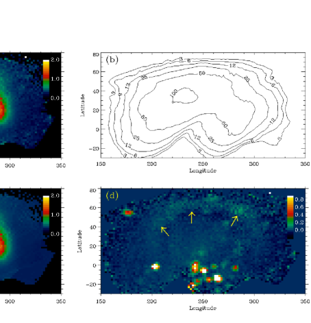
Figure 1: (a) Map of average count rates observed by Ulysses/GAS for 238 WFOV He beam maps observed throughout the mission, in ecliptic coordinates. Point sources are UV-bright stars. The horseshoe-shaped streak is the track of the He beam across the sky during the course of Ulysses’s orbit around the Sun. (b) Contour plot indicating the number of individual maps that actually sample each grid point. (c) Reconstruction of the coadded count rate map in (a) based on the best-fit He flow parameters and background values from WMW15. (d) Residual map after subtracting (c) from (a). Yellow arrows identify the residual signal that is interpreted as being from secondary He neutrals.

Thus, in searching for the secondary signal, we first coadd all 238 beam maps. The individual maps are irregularly gridded in ecliptic coordinates, but we map them onto a regular grid, with a grid point size of $2^{\circ}\times 2^{\circ}$. At each grid point, $i$, we determine the average count rate observed at that point for the set of beam maps that actually sample that location, $S_{i}$. By keeping track of the effective exposure time for each bin, $t_{i}$, we can also compute the Poissonian uncertainties of the $S_{i}$ count rates, $\sigma_{i}=\sqrt{S_{i}t_{i}}/t_{i}$. The resulting map of $S_{i}$ count rates is shown in Figure 1(a). The point sources in the map are UV-bright stars, as the GAS instrument possesses some degree of UV sensitivity. But the primary signal apparent in the image is a horseshoe-shaped feature, which represents the track of the primary He beam across the sky, as Ulysses’s position and motion vector change during the course of its orbit. When the ISM He atoms become visible at the beginning of a fast latitude scan, with Ulysses south of the ecliptic plane, the beam is observed at the right end of the horseshoe, near ($\lambda$,$\beta$)=($285^{\circ}$,$10^{\circ}$). The beam then shifts upwards to about ($280^{\circ}$,$45^{\circ}$) at the ecliptic plane crossing. With Ulysses moving north of the ecliptic and ultimately away from the Sun, the beam then shifts to the left and then ultimately downwards, ending up at the left end of the horseshoe near ($220^{\circ}$,$10^{\circ}$), when the He atoms become unobservable again.

In interpreting Figure 1(a), it is worth noting again that each grid point is the average count rate observed at that point for all maps that include that point, including maps where that point is actually outside the location of the beam at that time. Furthermore, we are mapping irregularly gridded points onto a regular grid, so adjacent points can actually be sampled by a different fraction of on-beam to off-beam maps. This is the primary reason for the pixel-to-pixel variation within the beam, not Poissonian noise. Likewise, the intensity variation along the horseshoe-shaped beam is mostly an indication of different parts of the horseshoe being sampled by a different number and fraction of on-beam maps. For example, the gap in the horseshoe at about ($280^{\circ}$,$40^{\circ}$) is a location where there are relatively few on-beam maps (see Figure 3(a) in WMW15), so the available count rate measurements for that location include mostly off-beam measurements. Thus, the average count rate there ends up low. Figure 1(b) is a contour plot showing the number of maps sampled at each point in the grid. Within the horseshoe-shaped track, each point is typically sampled by $50-100$ individual maps, out of the 238 total considered. The middle of the horseshoe is similarly well sampled, but the sampling falls off quickly outside the horseshoe.

In searching for a secondary signal, the first step is to subtract the primary beam from the data. In WMW15, we performed a global fit to the primary He neutrals observed in the 238 maps, deriving a best-fit He flow vector, and best-fit synthetic beam maps. Each of these individual maps assumes a flat background underneath the beam, and these backgrounds are free paramters of the global fit. We can coadd the synthetic He beam and background maps in the same way as we coadded the actual beam maps to yield maps of primary beam count rates, $C_{1,i}$, and model background, $B_{i}$. The sum, $C_{1,i}+B_{i}$, is shown in Figure 1(c). Figure 1(d) shows the residual after subtracting Figure 1(c) from Figure 1(a), $S_{2,i}=S_{i}-C_{1,i}-B_{i}$. This is now a map in which we can actually search for a signal from the secondary He flow.

There does seem to be an excess signal after the subtraction of the primary beam, identified by arrows in Figure 1(d). We claim this to be a likely Ulysses detection of the “Warm Breeze” neutrals first observed by IBEX. In their fit of the neutrals, Kubiak et al. (2016) find a much slower flow speed of $V=11.3$ km s^-1 compared to the $V=26.08$ km s^-1 flow of the primary He component (WMW15). In Ulysses data, a slower flow should lead to a significantly larger horseshoe-shaped track than that of the primary He beam (see Figure 7 in WMW15). Thus, based on the Kubiak et al. (2016) fit, the expectation is that in Figure 1 the secondary He component should be visible as a faint large horseshoe surrounding the bright smaller horseshoe of the primary component. This is a reasonable description of the residual signal seen in Figure 1(d), though the “legs” of the horseshoe are not as visible. It is also worth noting that the set of images that defines the residual signal at one location within the horseshoe will be very different from the set of images that defines the signal at a very different location within the horseshoe. It is impressive that a coherent horseshoe shape in Figure 1(d) emerges from beam maps that individually contribute to only one part of the horseshoe.

3 Fitting the Ulysses Secondary Helium Component

We now fit the Ulysses secondary He component, using techniques analogous to those used previously to fit the primary component, assuming a laminar, Maxwellian flow from infinity (WMW15). We have already noted in Section 1 that the laminar flow assumption is a poor one for the secondary He, but there are two reasons for keeping it for now. The first is simplicity, as it allows the secondary signal to be modeled using the same codes used to analyze the primary He beam. The second reason is that we want to be able to compare our Ulysses results with IBEX, and the IBEX secondary He flow properties are currently inferred assuming a laminar flow (Kubiak et al., 2016).

The five fit parameters are flow speed ($V$), flow longitude ($\lambda$) flow latitude($\beta$), temperature ($T$), and density far from the Sun ($n_{\rm He}$). One difference is that because it is very difficult to visually see the secondary signal in individual beam maps, we fit the coadded residual count rate map, $S_{2,i}$, rather than the direct Ulysses measurements in the individual maps, which was the approach in fitting the primary beam. We refer the reader to Section 4 of WMW15 for details about the particle tracking approach and synthetic map generation. After the 238 synthetic beam maps are created, they are coadded as the observed maps were coadded in Figure 1, in order to compare with the residual signal in Figure 1(d). The best fit is determined by minimizing the $\chi^{2}$ statistic (Bevington & Robinson, 1992). The average 1 AU photoionization rate for the 238 Ulysses maps under consideration is $\beta_{ion}=1.5\times 10^{-7}$ s^-1 (WMW15, see Section 5), so we simply assume that value in our calculations.

The WMW15 analysis did not consider the contribution of the secondary neutrals to the background, and therefore the true background may have been overestimated, meaning Figure 1(d) could be underestimating the secondary signal. In order to correct for this, we first perform a preliminary fit to the secondary signal. We then use the best-fit secondary He flow parameters to compute the secondary count rates within the 238 original Ulysses beam maps. Subtracting the secondary counts from these maps, we then redo the WMW15 analysis of the primary beam. This accomplishes two things. The first is to see whether correcting for the secondaries in any way affects the fit parameters of the primary He flow. The answer is that it does not. The secondary signal is too weak to significantly affect the fit to the primary neutrals. The second accomplishment is revised measurements of the background levels in the individual 238 maps, which we can use to create a revised $B_{i}$ background map. The average background of the 238 maps is 0.384 cts s^-1, which is not that different from the original measurements (see Figure 8(b) in WMW15).

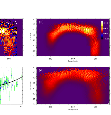
Figure 2: (a) A map of residual counts after subtracting the primary beam and background counts, zooming in on only the pixels around the He secondary signal that are being fitted. (b) Average count rate map based on the best He flow vector fit to the data in (a). (c) Observed versus model count rates based on the best He flow vector fit, with the thick black line being the line of agreement. A log scale is used for the x-axis to spread out the low count values. (d) Average count rate map expected based on the He secondary flow vector inferred from IBEX data (Kubiak et al. 2016). Note that the count rate color scale in (b) applies to all the count rate map panels.

We recompute the residual map, $S_{2,i}$, using the revised background estimates. Figure 2(a) displays the revised $S_{2,i}$ map, which is not greatly different from that in Figure 1(d). The figure zooms in on the region around the secondary signal, identifying the pixels in the map used in our fits. A new and final fit is performed to this count rate map. Figure 2(b) shows the count rate map of our best fit to the data, which we denote as $C_{2,i}$. Figure 2(c) explicitly compares the observed and modeled count rates in this fit. Typical count rates within the horseshoe-shaped secondary He beam track are $0.05-0.10$ cts s^-1. This is a factor of 4 to 8 lower than the background ($B_{i}$) and a factor of 20 to 40 lower than typical count rates within the primary beam track ($C_{1,i}$), both of which have been subtracted from the data to yield the residual signal in Figure 2(a). In addition to roughly reproducing the shape and width of the horeshoe-shaped track, it is encouraging that the fit reproduces the bright spot on this track observed at ($\lambda$,$\beta$)=($285^{\circ}$,$60^{\circ}$), which has no real analog on the primary beam track (see Figure 1). There is, therefore, a strong case for this being a real feature. Finally, Figure 2(d) shows the secondary He signal predicted by the IBEX-derived “Warm Breeze” flow vector described in Section 1.

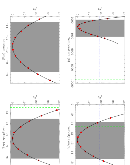
Figure 3: Secondary helium flow parameter measurements from a fit to the Ulysses coadded count rate residual map in Figure 2(a). In each panel, $\Delta\chi^{2}$ is plotted as a function of one of the four He flow parameters of interest, where each point represents a separate fit with that parameter held constant and the other three parameters (and the He density) allowed to vary freely. Solid lines show polynomial fits to the data points. The horizontal dot-dashed line corresponds to the $3\sigma$ contour used to define the uncertainty range in each parameter (shaded regions). Vertical dashed lines are the Kubiak et al. (2016) measurements from IBEX data.

Determining the best fit parameters and their uncertainties requires computing a grid of fits. Figure 3 shows how $\chi^{2}$ varies when $T$, $V$, $\beta$, and $\lambda$ are held constant. The $\chi^{2}$ statistic is well-behaved, showing a clear $\chi^{2}$ minimum, $\chi^{2}_{min}$, in each panel. If $\nu$ is the number of degrees of freedom of the fit (the number of data points minus the number of free parameters), then the reduced chi-squared is defined as $\chi^{2}_{\nu}=\chi^{2}/\nu$, which should be $\sim 1$ for a good fit. For our fit, $\nu=1721$ and $\chi^{2}_{{\nu},min}=2.397$. We define $\Delta\chi^{2}\equiv\chi^{2}-\chi^{2}_{min}$, with each panel of Figure 3 showing the variation of $\Delta\chi^{2}$ across the $\chi^{2}_{min}$ region. Third order polynomials are fitted to the data points to interpolate between them.

The $\Delta\chi^{2}$ values are used to define the error bounds around $\chi^{2}_{min}$, as described by Bevington & Robinson (1992) and Press et al. (1989). For the number of free parameters of our fit (five), the $3\sigma$ confidence contour corresponds to $\Delta\chi^{2}=18.2$, based on relation 26.4.14 of Abramowitz & Stegun (1965), and this level defines the uncertainty ranges shown in Figure 3. Our derived secondary He flow parameters are: $V=12.8\pm 1.9$ km s^-1, $\lambda=74.4\pm 1.8^{\circ}$, $\beta=-10.5\pm 4.1^{\circ}$, and $T=3000\pm 1100$ K. At this point it should be noted that Ulysses data are provided in B1950 coordinates, and the analysis is performed in those coordinates, but the coordinates we quote in this paper are always converted to the now more standard J2000 epoch.

In Figure 3, the Ulysses-derived flow parameters are compared with those from IBEX data, also listed in Section 1. The $V$ and $\beta$ values are in good agreement. There is a small inconsistency in $\lambda$, but if the total statistical plus systematic uncertainty in the IBEX measurement ($0.5^{\circ}+0.9^{\circ}=1.4^{\circ}$) is considered (Kubiak et al., 2016), the IBEX and Ulysses error bars will overlap. The only serious disagreement is temperature, $T$, for which there is a very large discrepancy. Figure 2(d) shows how the larger $T$ of the IBEX secondary parameters leads to a broader horseshoe than observed. For example, there is significant predicted flux at ($\lambda$,$\beta$)=($200^{\circ}$,$60^{\circ}$) and ($300^{\circ}$,$70^{\circ}$), which does not seem to be observed in Figure 2(a). The relatively narrow observed horseshoe-shaped track seems to require a surprisingly low temperature of $T\approx 3000$ K.

Before discussing the temperature issue further, there is one final fit parameter to discuss, the density. For the fits in Figure 3 that fall within the error bars, we compute the mean and standard deviation of the He densities inferred from these individual fits, leading to our best estimate of the He density of the secondary component, $n_{\rm He}=(9.6\pm 0.7)\times 10^{-4}$ cm^-3. Dividing this by the best estimate of the primary component density from WMW15, $n_{\rm He}=0.0196$ cm^-3, we find that the secondary component is $4.9\pm 0.9$% of the primary component, in good agreement with the 5.7% measurement from IBEX. Four of the five Ulysses secondary He flow parameters are therefore in reasonably good agreement with IBEX measurements, providing support for the detection of the “Warm Breeze” neutrals by Ulysses.

It is only the temperature that seems inconsistent. The IBEX-derived $T=9500$ K temperature was already recognized to be problematic, being well below the $T\approx 20,000$ K temperatures expected for the outer heliosheath source region of the secondary He neutrals. Our Ulysses measurement of $T=3000$ K represents an even larger underestimate. The implausibly low temperature measurements are a consequence of the improper approximation of the secondary neutral flow as being laminar beyond the heliopause, as opposed to a divergent flow due to deflection around the heliopause.

This was demonstrated explicitly by Wood (2017), who used a simple 2-D model of a divergent flow field to explore how the angular width of the observed He beam observed near 1 AU, $W$, relates to flow velocity, $V$, temperature, $T$, and flow divergence, $D$, in the outer heliosheath source region. The flow pattern at the outer boundary is defined by the simple equation $\psi=D\times\theta$, where $\theta$ is the viewing angle from the upwind direction of the ISM flow, and $\psi$ is the deviation of flow direction from the ISM flow direction. So if $D=0.5$, at an angular distance of $\theta=30^{\circ}$ from the upwind direction the flow would be diverging by $\psi=15^{\circ}$ from the direction of the ISM flow (see Figure 1 of Wood 2017). It was shown that $W$, $V$, $T$, and $D$ could be related by the power law relation

$$W=C\left(\frac{V}{20}\right)^{\alpha}\left(\frac{T}{10^{4}}\right)^{\beta}\left(D+1\right)^{\gamma},$$ (1)

with $V$ in km s^-1 and $T$ in K. For the case with an observer at 1 AU along the stagnation axis, $C=24.1^{\circ}$, $\alpha=-0.84$, $\beta=0.52$, and $\gamma=-0.91$.

Applying equation (1), the Ulysses fit to the secondaries, ($D$,$T$,$V$)=(0,3000,12.8), would predict a He beam width of $W=18.7^{\circ}$ in the context of the simple 2-D model. Global heliospheric models suggest $V\approx 9$ km s^-1 and $T\approx 21,000$ K for the outer heliosheath (Kubiak et al., 2014; Izmodenov & Alexashov, 2015). Assuming these values for $V$ and $T$, equation (1) can then be used to compute the value of $D$ necessary to recover the $W=18.7^{\circ}$ width that is crudely representative of the Ulysses measurements. The resulting divergence is $D=3.2$. The point is that a sufficiently divergent flow can explain the low temperature measurement. Equation (1) and the values of the power law indices quoted above will not be precisely applicable to either the Ulysses or IBEX cases, as the 2-D model does not accurately replicate the observing geometries of either, but we use them here simply to illustrate how switching from a laminar to a divergent flow should naturally lead to higher and more plausible temperatures.

This does not necessarily explain why the Ulysses temperature measurement is so much lower than the IBEX measurement. Is it possible that the Ulysses data are more sensitive to the effects of a divergent flow than IBEX? This could in principle be the case, given the very different observing geometries of Ulysses and IBEX, and the energy-dependent sensitivity of the Ulysses/GAS detector, which is unlike the IBEX detector. Exploring this further would require fitting the IBEX and Ulysses data again assuming a divergent flow rather than a laminar one, to see if such an assumption would not only lead to higher and more plausible $T$ measurements, but would also resolve the IBEX/Ulysses discrepancy. Such a task is beyond the scope of the present analysis.

Another concern particular to the Ulysses measurement is the issue of background subtraction. Discussion of Ulysses background sources can be found in Witte et al. (1993) and Banaszkiewicz et al. (1996). The secondary signal is significantly weaker than the background, so inaccuracies in the background subtraction represent a significant source of systematic uncertainty in the analysis. Hints of inaccuracies are apparent in Figure 2(a), where residual count rates outside the secondary signal seem preferentially negative, when they should be zero on average. We compute an average count rate of $-0.008$ cts s^-1 outside the secondary signal in Figure 2(a), suggesting that our background map, $B_{i}$, may be $\sim 2$% too high in the vicinity of the secondary signal.

Our analysis of the primary He beam assumes a flat background under the He beam in each of the 238 individual beam maps. In order to explore whether the flat background assumption might be affecting our results, we redid the analysis allowing the background to vary in a linear fashion underneath the beam. However, the resulting coadded background map, $B_{i}$, does not end up looking very different from the coadded map assuming flat backgrounds, and the residual maps $S_{2,i}$ shown in Figures 1(d) and 2(a) therefore do not look very different either. Thus, the assumption of a non-flat background does not significantly affect the secondary flow fit parameters.

In a final effort to see if we can improve agreement with the IBEX measurements, we conduct the following experiment. We described above how we revised the background measurements from WMW15 for the individual 238 Ulysses maps using a preliminary fit to the $S_{2,i}$ residual map to account for the secondary neutrals. We repeat this revision, but we instead use the IBEX He flow parameters to estimate the secondary neutral count rates, analogous to how Figure 2(d) was computed. This leads to a revised measurement of the background map, $B_{i}$, and a revised $S_{2,i}$ residual map. We are essentially trying to bias the analysis towards ultimately yielding a residual map that looks more like Figure 2(d) than Figure 2(a). However, results are once again not much different than before, and when we fit the resulting residual map, there is no significant change in the fit parameters. Thus, this test fails to provide evidence that background uncertainties are responsible for the $T$ discrepancy with IBEX.

4 Deflection from the ISM Flow Direction

Possibly the strongest evidence that the “Warm Breeze” neutrals detected by IBEX are created by charge exchange in the outer heliosheath is that the flow direction of the “Warm Breeze” neutrals lies between the ISM flow direction and the direction of the ISM magnetic field. The idea is that the ISM field creates asymmetries in the heliopause and the flow around the heliopause, such that neutrals created by charge exchange outside the heliopause will appear to be deflected from the ISM flow direction towards the direction of the ISM magnetic field (Izmodenov et al., 2005; Opher et al., 2007; Pogorelov et al., 2008).

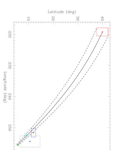
Figure 4: A map in ecliptic coordinates showing the assumed direction of the local ISM magnetic field based on the center of the IBEX ribbon (red box; Funsten et al. 2013), the upwind direction of the ISM He flow (green box; WMW15), the upwind direction of the H flow in the solar system (light blue box; Lallement et al. 2005, 2010), the IBEX-derived upwind direction of the secondary He flow (solid blue box; Kubiak et al. 2016), and the Ulysses-derived upwind direction of the secondary He flow (dotted blue box; this paper). The boxes indicate the quoted uncertainties in the directions. The ISM velocity and field directions define a plane whose intersection with the map is shown as a great circle line connecting the velocity and field directions, with uncertainties indicated by dashed lines. The expectation is that the H and secondary He flows should be on this line.

In Figure 4, we plot in ecliptic coordinates the ISM field direction inferred from the IBEX ribbon center (Funsten et al., 2013) and the upwind ISM flow direction from WMW15, with the connecting line indicating the path along a great circle connecting the two. The secondary He neutral flow direction should lie on this line. The He secondary flow directions from both IBEX (Kubiak et al., 2016) and Ulysses are shown, and both IBEX and Ulysses boxes overlap the line, albeit in different locations. Likewise, the expectation is that the H flow direction measured by the SWAN instrument on SOHO should also lie along this line, as the observed flow should include many H neutrals created by charge exchange beyond the heliopause. The SOHO/SWAN measurements of the H flow are shown in Figure 4 (Lallement et al., 2005, 2010), demonstrating that the H flow does indeed lie nicely on the line.

The IBEX-derived flow direction has lower uncertainties and is closer to the expected line of deflection than our Ulysses measurement. For the primary ISM He flow, we actually found that Ulysses constraints on the He flow vector are tighter than those of IBEX despite lower S/N (WMW15, Wood & Müller, 2015). This is due to the Ulysses advantage of observing the He flow at different locations and with different spacecraft motion vectors, which effectively breaks the parameter degeneracies that plague analysis of IBEX data. However, for the fainter secondary component, it is likely that the superior S/N of IBEX is more important and will lead to tighter constraints on the secondary flow vector. Still, the Ulysses data provide a useful independent confirmation of the existence and general characteristics of the secondary He flow in the inner heliosphere.

5 Summary

We have analyzed Ulysses/GAS observations of neutral He flowing through the solar systeam to search for a signature of the “Warm Breeze” neutrals detected by IBEX, and our results are summarized as follows:

1. By coadding the Ulysses He maps together to maximize S/N, and then subtracting the signal from the primary He neutrals and the background, we are able to find a weak residual signal that represents a likely detection of the secondary He neutrals first detected by IBEX.

2. We estimate the secondary He flow vector by fitting the residual signal assuming a laminar flow at infinity, yielding the following fit parameters: $V=12.8\pm 1.9$ km s^-1, $\lambda=74.4\pm 1.8^{\circ}$, $\beta=-10.5\pm 4.1^{\circ}$, and $T=3000\pm 1100$ K; with a density $4.9\pm 0.9$% that of the primary ISM He component. Most of these values are in reasonable agreement with IBEX measurements (Kubiak et al., 2016), which were also based on the laminar flow at infinity approximation. The one discrepant parameter is temperature, where our value is much lower than the IBEX-derived $T=9500$ K. Both the IBEX and Ulysses temperatures are significantly lower than those expected to actually exist in the outer heliosheath. The underestimates most probably will be due to the assumption of a laminar flow at the outer boundary, as opposed to the divergent flow that will actually exist there.

3. The reason for the discrepant $T$ measurement is uncertain at this time, but it could also be due to background subtraction uncertainties for Ulysses (Witte et al., 1993; Banaszkiewicz et al., 1996), or it could be associated with the inadequate and imprecise assumption that the He secondaries can be approximated as a laminar flow from infinity, which could in principle affect the IBEX and Ulysses data differently.

The He secondary flow is a unique diagnostic of the outer heliosheath that may prove to be the best way to remotely study the deflection of the ISM flow around the heliopause. The biggest problem with existing analyses of the secondary He is the approximation of the flow as a laminar flow from infinity. Future analyses should instead assume a parametrized divergent flow from about 150 AU. This should lead to more accurate inferences of the flow properties in the outer heliosheath, including a higher and more realistic temperature. It remains to be seen if such an analysis will resolve the $T$ discrepancy between IBEX and Ulysses reported here.

References

- Abramowitz & Stegun (1965) Abramowitz, M., & Stegun, I. A. 1965, Handbook of Mathematical Functions (New York: Dover Publications, Inc.)
- Banaszkiewicz et al. (1996) Banaszkiewicz, M., Witte, M., & Rosenbauer, H. 1996, A&AS, 120, 587
- Bevington & Robinson (1992) Bevington, P. R., & Robinson, D. K. 1992, Data Reduction and Error Analysis for the Physical Sciences (New York: McGraw-Hill)
- Bzowski et al. (2017) Bzowski, M., Kubiak, M. A., Czechowski, A., & Grygorczuk, J. 2017, ApJ, 845, 15
- Bzowski et al. (2014) Bzowski, M., Kubiak, M. A., Hlond, M., et al. 2014, A&A, 569, A8
- Bzowski et al. (2012) Bzowski, M., Kubiak, M. A., Möbius, E., et al. 2012, ApJS, 198, 12
- Frisch et al. (2013) Frisch, P. C., et al. 2013, Science, 341, 1080
- Funsten et al. (2013) Funsten, H. O., DeMajistre, R., Frisch, P. C., et al. 2013, ApJ, 776, 30
- Izmodenov & Alexashov (2015) Izmodenov, V. V., & Alexashov, D. B. 2015, ApJS, 220, 32
- Izmodenov et al. (2005) Izmodenov, V., Alexashov, D., & Myasnikov, A. 2005, A&A, 437, L35
- Izmodenov et al. (2003) Izmodenov, V., Malama, Y. G., Gloeckler, G., & Geiss, J. 2003, ApJ, 594, L59
- Katushkina et al. (2014) Katushkina, O. A., Izmodenov, V. V., Wood, B. E., & McMullin, D. R. 2014, ApJ, 789, 80
- Kubiak et al. (2014) Kubiak, M. A., Bzowski, M., Sokól, J. M., et al. 2014, ApJS, 213, 29
- Kubiak et al. (2016) Kubiak, M. A., Swaczyna, P., Bzowski, M., et al. 2016, ApJS, 223, 25
- Lallement et al. (2005) Lallement, R., Quémerais, E., Bertaux, J. L., et al. 2005, Science, 307, 1447
- Lallement et al. (2010) Lallement, R., Quémerais, E., Koutroumpa, D., et al. 2010, in Solar Wind 12, ed. M. Maksimovic et al. (Melville, NY: AIP), 555
- McComas et al. (2009) McComas, D. J., Allegrini, G., Bochsler, P., et al. 2009, Space Sci. Rev., 146, 11
- McComas et al. (2015) McComas, D. J., Bzowski, M., Frisch, P., et al. 2015, ApJ, 801, 28
- Möbius et al. (2012) Möbius, E., Bochsler, P., Bzowski, M., et al. 2012, ApJS, 198, 11
- Müller et al. (2013) Müller, H. -R., Bzowski, M., Möbius, E., & Zank, G. P. 2013, in Solar Wind 13, ed. G. P. Zank, et al. (New York: AIP, Vol. 1539), 348
- Opher et al. (2007) Opher, M., Stone, E. C., & Gombosi, T. I. 2007, Science, 316, 875
- Park et al. (2016) Park, J., Kucharek, H., Möbius, E., et al. 2016, ApJ, 833, 130
- Pogorelov et al. (2008) Pogorelov, N. V., Heerikhuisen, J., & Zank, G. P. 2008, ApJ, 675, L41
- Press et al. (1989) Press, W. H., Flannery, B. P., Teukolsky, S. A., & Vetterling, W. T. 1989, Numerical Recipes (Cambridge: Cambridge University Press)
- Schwadron et al. (2016) Schwadron, N. A., Möbius, E., McComas, D. J., et al. 2016, ApJ, 828, 81
- Sokół et al. (2015) Sokół, J .M., Kubiak, M. A., Bzowski, M., & Swaczyna, P. 2015, ApJS, 220, 27
- Wenzel et al. (1992) Wenzel, K. -P., Marsden, R. G., Page, D. E., & Smith, E. J. 1992, A&AS, 92, 207
- Witte (2004) Witte, M. 2004, A&A, 426, 835
- Witte et al. (1996) Witte, M., Banaszkiewicz, M., & Rosenbauer, H. 1996, Space Sci. Rev., 78, 289
- Witte et al. (1993) Witte, M., Rosenbauer, H., Banaszkiewicz, M., & Fahr, H. 1993, Adv. Space Res., 13, 121
- Witte et al. (1992) Witte, M., Rosenbauer, H., Keppler, E., Fahr, H., Hemmerich, P., Lauche, H., Loidl, A., & Zwick, R. 1992, A&AS, 92, 333
- Wood (2017) Wood, B. E. 2017, in 16th Annual International Astrophysics Conference: Turbulence, Structures, and Particle Acceleration Throughout the Heliosphere and Beyond, J. of Phys. Conf. Ser., 900, 012021
- Wood & Müller (2015) Wood, B. E, & Müller, H. -R. 2015, in 14th Annual International Astrophysics Conference: Linear and Nonlinear Particle Energization Throughout the Heliosphere and Beyond, J. of Phys. Conf. Ser., 642, 012029
- Wood et al. (2015) Wood, B. E., Müller, H. -R., & Witte, M. 2015, ApJ, 801, 62 (WMW15)
- Zank et al. (2013) Zank, G. P., Heerikhuisen, J., Wood, B. E., et al. 2013, ApJ, 763, 20