Spatio-Temporal Data Mining: A Survey of Problems and Methods

Abstract.

Large volumes of spatio-temporal data are increasingly collected and studied in diverse domains including, climate science, social sciences, neuroscience, epidemiology, transportation, mobile health, and Earth sciences. Spatio-temporal data differs from relational data for which computational approaches are developed in the data mining community for multiple decades, in that both spatial and temporal attributes are available in addition to the actual measurements/attributes. The presence of these attributes introduces additional challenges that needs to be dealt with. Approaches for mining spatio-temporal data have been studied for over a decade in the data mining community. In this article we present a broad survey of this relatively young field of spatio-temporal data mining. We discuss different types of spatio-temporal data and the relevant data mining questions that arise in the context of analyzing each of these datasets. Based on the nature of the data mining problem studied, we classify literature on spatio-temporal data mining into six major categories: clustering, predictive learning, change detection, frequent pattern mining, anomaly detection, and relationship mining. We discuss the various forms of spatio-temporal data mining problems in each of these categories.

1. Introduction

Space and time are ubiquitous aspects of observations in a number of domains, including, climate science, neuroscience, social sciences, epidemiology, transportation, criminology, and Earth sciences, that are rapidly being transformed by the deluge of data. Since the real-world processes being studied in these domains are inherently spatio-temporal in nature, a number of data collection methodologies have been devised to record the spatial and temporal information of every measurement in the data, hereby referred to as spatio-temporal (ST) data. For example, in neuroimaging data, activity measured from the human brain is stored along with the spatial location from which the activity was measured and the time at which the measurement was made. Similarly, web-search requests arriving at Google’s servers have a geographic location and time from which they are made. Effective analysis of such increasingly prevalent ST data holds great promise for advancing the state-of-the-art in several scientific disciplines.

A unique quality of ST data that differentiates it from other data studied in classical data mining literature (e.g., see (Tan et al., 2017)) is the presence of dependencies among measurements induced by the spatial and temporal dimensions. For example, many of the widely used data mining methods are founded on the assumption that data instances are independent and identically distributed ($i.i.d$). However, this assumption is violated when dealing with ST data, where instances are structurally related to each other in the context of space and time and show varying properties in different spatial regions and time periods. Ignoring these dependencies during data analysis can lead to poor accuracy and interpretability of results (Eklund et al., 2016).

Apart from limiting the effectiveness of classical data mining algorithms, the presence of spatial and temporal information also makes it possible to consider novel formulations for analyzing data in the emerging field of spatio-temporal data mining (STDM). Contrary to traditional data mining that deals with distinct objects (also referred to as data instances) having well-defined features, in STDM, one can define objects and features in a variety of ways. One scenario involves treating spatial locations as objects and using the measurements collected from a spatial location over time to define the features. For example, in climate science, one of the goals is to group locations that experience similar climatic phenomenon over time. In this case, locations are treated as instances/objects and features are defined based on climate variables measured over time (Steinbach et al., 2002). Another scenario involves treating time points as objects and using measurements collected from all the spatial locations under consideration to define features. For example, in the application of discovering patterns of human brain activity from neuroimages, the goal is to identify the time points at which similar brain activity is observed in the brain. In this case, time points are treated as objects/instances and features are defined using the observed spatial map of activity (Liu et al., 2013). There are also scenarios where events are treated as objects and features are defined based on the spatial and temporal information of events. For example, in the context of discovering crimes that are committed in close proximity in space and time, incidence of a crime is treated as an object and the location and time stamp of the crime are treated as features, in addition to other features such as nature of crime and number of victims involved (Tompson et al., 2015). Hence, the coupling of spatial and temporal information in ST data introduces novel problems, challenges, and opportunities for STDM research, with a broad scope of application in several domains of scientific and commercial significance.

There exists a vast literature on approaches for mining data that is purely spatial in nature, spanning multiple decades of research in spatial statistics (Cressie and Wikle, 2015), spatial data mining (Shekhar et al., 2008, 2011; Aggarwal, 2015), and spatial database management (Ester et al., 1997; Shekhar and Chawla, 2003). An extensive taxonomy of spatial data types and representations has been explored in the field of spatial data mining for improving the efficiency and effectiveness of data mining tasks such as clustering, prediction, anomaly detection, and pattern mining when dealing with spatial data (Shekhar et al., 2011). Another related area of research is time series data mining (Keogh and Kasetty, 2003; Liao, 2005; Esling and Agon, 2012), where approaches for mining useful information from time-series databases have been explored. Existing research in STDM includes foundational research in the statistics community (Cressie and Wikle, 2015), e.g., research on spatio-temporal point processes (Diggle, 2013). Approaches for handling spatial and temporal information have also been explored in the data mining literature for problems such as spatio-temporal clustering (Kisilevich et al., 2010) and trajectory pattern mining (Giannotti et al., 2007).

There are a few recent surveys that have reviewed the literature on STDM in certain contexts from different perspectives. Articles by (Vatsavai et al., 2012) and (Chandola et al., 2015) discuss the computational issues for STDM algorithms in the era of ‘big-data’ for application domains such as remote sensing, climate science, and social media analysis. The review by (Cheng et al., 2014) covers STDM approaches for prediction, clustering, and visualization problems in several applications. An extensive survey of approaches for mining trajectory data, one of the many types of ST data, is presented in (Li, 2014; Zheng, 2015; Mamoulis, 2009). A survey on STDM by (Shekhar et al., 2015) provides a semantic categorization of ST data types and pattern families from a database-centric perspective.

Given the richness of problems and the variety of methods being explored in the rapidly advancing field of STDM, there is a need for developing an over-arching structure of research in STDM that highlights the similarities and differences of different problems and methods in diverse ST applications. This can enable the cross-pollination of ideas across disparate research areas and application domains, by making it possible to see how a solution developed for a certain problem in a particular domain (e.g., identifying patterns in climate data) can be useful for solving a different problem in another domain (e.g., understanding the working of the brain). This can also help in connecting the traditional data mining community with the challenges and opportunities in analyzing ST data, thus exposing some of the open questions and motivating future directions of research in STDM.

This review paper on STDM problems and methods attempts to fulfill this need as follows. First, it builds a foundation of ST data types and properties that can help in identifying the relevant problems and methods for any class of ST data encountered in real-world applications. In particular, we provide a broad taxonomy of the different types of ST data, different ways of defining and describing ST data instances, and different ways of computing similarity among ST data instances. Second, it presents a survey of STDM approaches for a number of commonly studied data mining problems such as clustering, predictive learning, frequent pattern mining, anomaly detection, change detection, and relationship mining. For every category of problems, we review the novel issues that arise in dealing with the unique properties of ST data types in classical data mining frameworks. This paper can be used as a guide by data mining researchers and real-world practitioners working with ST data, to identify STDM formulations fit for their data and to make most effective use of STDM research in their problem. In addition, by bridging the gap between classical data mining literature and the novel aspects of spatio-temporal data, this paper helps in opening novel possibilities of future research.

The rest of the paper is organized as follows. In Section 2 we review the variety of application areas where analyzing ST data is important. In Section 3, we discuss the types and characteristics of ST data, and the different ways of defining instances and similarity measures using ST data types. Section 4 presents a survey of STDM methods developed for different types of ST data instances in the context of six major data mining problems, viz., clustering, predictive learning, frequent pattern mining, anomaly detection, change detection, and relationship mining. Section 5 presents concluding remarks and discusses future research directions.

2. Applications

Large volumes of ST data are collected in several application domains such as social media, health-care, agriculture, transportation, and climate science. In this section, we briefly describe the different sources of ST data and the motivation for analyzing ST data in different application domains.

Climate Science: Data pertaining to historic and current atmospheric and oceanic conditions (e.g., temperature, pressure, wind-flow, and humidity) is collected and studied in climate science (Karpatne et al., 2013). In addition to observational data collected from weather stations and reanalysis data that is gridded in space (Kistler et al., 2001), simulated data generated using climate models (Voldoire et al., 2013) is also studied in this domain. The purpose in studying this data is to discover relationships and patterns in climate science that advance our understanding of the Earth’s system and help us better prepare for future adverse conditions by informing adaptation and mitigation actions in a timely manner.

Neuroscience: Continuous neural activity captured using a variety of technologies such as Functional Magnetic Resonance Imaging (fMRI), Electroencephalogram (EEG), and Magnetoencephalography (MEG) is studied in neuroscience (Atluri et al., 2016). Spatial resolution of neural activity measured using these technologies is quite different from another. For example, neural activity is measured from millions of locations in fMRI data, while it is only measured from tens of locations in the case of EEG data. Temporal resolution of the data collected using these technologies is also quite different. For example, fMRI typically measures activity for every two seconds, while the temporal resolution of EEG data is is typically 1 millisecond. The purpose in studying this data is to understand the governing principles of the brain and thereby determine the disruptions to normal conditions that arise in the case of mental disorders (Atluri et al., 2015; Atluri et al., 2013). Discovering such disruptions can be useful for designing diagnostic procedures and in developing therapeutic procedures for patients.

Environmental Science: Studying the data pertaining to the quality of air, water, and environment is one of the objectives of environmental science. While air quality is measured based on the presence of pollutants such as particles, carbon monoxide, nitrogen dioxide, sulphur dioxide, ozone etc., water quality is measured based on factors such as dissolved oxygen, conductivity, turbidity, and pH. Air quality sensors are typically placed on streets or on top of buildings, and water quality sensors are placed in lakes, rivers, and streams. In addition to air and water quality, data pertaining to sound pollution is also collected. These environmental data sets are studied to detect changes in levels of pollution, identify the causal factors that contribute to pollution, and to design effective policies to reduce the different types of pollution (Thompson et al., 2014).

Precision Agriculture: Multi-band high-resolution (ranging from 0.25m to 1m) areal or remote-sensing images of large farms are being collected at regular intervals (e.g., daily to weekly). One of the purposes of collecting and studying this data is to detect plant diseases (Mahlein, 2016) and understand the impact of several factors such as misapplication of fertilizer, compaction during planting and weeds on crop yield, as well as their inter-relationships. With the help of this knowledge, steps can be taken in future crop cycles to mitigate the risks due to the factors that adversely affect the crop yield.

Epidemiology/ Health care: Electronic health record data that is widely stored in hospitals provide demographic information pertaining to patients as well diagnosis made on patients at different time points. This dataset can be represented as a spatio-temporal dataset where each diagnosis has a spatial location and a time-point associated with it. One can construct such spatio-temporal instances for different types diseases such as cancers and diabetes, as well as for infectious diseases such as influenza. This data is studied to discover spatio-temporal patterns in different diseases (Matsubara et al., 2014) and to study the spread of an epidemic. This data is also used in conjunction with environmental, climate science data sets to discover relationships between environmental factors and public health (Ryan et al., 2007). Discovery of such relationships will allow policy-makers to develop effective policies that will ensure the well-being of the population.

Social media: Users of social media portals such as Twitter and Facebook post their experience at a given place and time. Each social media post captures the experience of a user at a given place and time. Using this data one can study collective user experience at a given place for a given time period (Tang et al., 2014). One can also capture the spread of epidemics such as Influenza or ebola based on users’ posts. More recently, there is also increased interest in studying the spread of social and political movements using social media data (Carney, 2016). In addition, events such as earthquakes, tsunamis, and fires can also be automatically detected from this data.

Traffic Dynamics: Large scale taxi pick-up/drop-off data is publicly available for several major cities across the world (Castro et al., 2013). This data contains information about each trip made by customers of the taxi service, including the time and location of pick-up and drop-off, and GPS locations for each second during the taxi ride. This data can be used to understand how the population in a city moves spatially as a function of time and also the influence of extraneous factors such as traffic and weather. In addition, this data can also be studied to explore traffic dynamics based on the collective movement patterns of the taxis. This will enable transportation engineers to design effective policies to reduce traffic congestion. In addition, the behavior of taxi drivers can also be studied using this data so effective practices can be designed to detect abnormal behavior, increasing likelihood of finding new passengers, and taking optimal routes to arrive at a destination.

Heliophysics: Heliophysics studies the events that occur in the Sun and their impact on the Solar System. The publicly available Heliophysics Events Knowledgebase (Hurlburt et al., 2010) provides various observations that include solar events and their annotations on a daily basis. Examples of these events include Active region, Emerging flux, Filament, Flare, Sigmoid, and Sunspot. The time and the location of where these events were observed on the Sun are also provided in the knowledgebase. The spatial and temporal information along with the different observations are studied to discover patterns in the solar events (Pillai et al., 2012). The Heliophysics knowledgebase also enables the study of the impact of solar events and the Earth’s climate system.

Crime data: Law enforcement agencies store information about reported crimes in many cities and this information is made publicly available in the spirit of open-data (Tompson et al., 2015). This data typically has the type of crime (e.g., arson, assault, burglary, robbery, theft, and vandalism), as well as the time and location of the crime. Patterns in crime and the effect of law enforcement policies on the amount of crime in a region can be studied using this data with the goal of reducing crime.

3. Data

The presence of space and time introduces a rich diversity of ST data types and representations, which leads to multiple ways of formulating STDM problems and methods. In this section, we first describe some of the generic properties of ST data, and then describe the basic types of ST data available in different applications. Building on this discussion, we describe some of the common ways of defining and representing ST data instances, and generic methods for computing similarity among different types of ST instances.

3.1. Properties

There are two generic properties of ST data that introduces challenges as well as opportunities for classical data mining algorithms, as described in the following.

3.1.1. Auto-correlation

In domains involving ST data, the observations made at nearby locations and time stamps are not independent but are correlated with each other. This auto-correlation in ST data sets results in a coherence of spatial observations (e.g., surface temperature values are consistent at nearby locations) and smoothness in temporal observations (e.g., changes in traffic activity occurs smoothly over time). As a result, classical data mining algorithms that assume independence among observations are not well-suited for ST applications, often resulting in poor performance with salt-and-pepper errors (Jiang et al., 2015). Further, standard evaluation schemes such as cross-validation may become invalid in the presence of ST data, because the test error rate can be contaminated by the training error rate when random sampling approaches are used to generate training and test sets that are correlated with each other. We also need novel ways of evaluating the predictions of STDM methods, because estimates of the location/time of an ST object (e.g., a crime event) may be useful even if they are not exact but in the close ST vicinity of ground-truth labels. Hence, there is a need to account for the structure of auto-correlation among observations while analyzing ST data sets.

3.1.2. Heterogeneity

Another basic assumption that is made by classical data mining formulations is the homogeneity (or stationarity) of instances, which implies that every instance belongs to the same population and is thus identically distributed. However, ST data sets can show heterogeneity (or non-stationarity) both in space and time in varying ways and levels. For example, satellite measurements of vegetation at a location on Earth show a cyclical pattern in time due to the presence of seasonal cycles. Hence, observations made in winter are differently distributed than the observations made in summer. There can also be inter-annual changes due to regime shifts in the Earth’s climate, e.g., El Nino phase transitions, which can impact climate patterns to change on a global scale. As another example, different spatial regions of the brain perform different functions and hence show varying physiological responses to a stimuli. This heterogeneity in space and time requires the learning of different models for varying spatio-temporal regions.

3.2. Data Types

There is a variety of ST data types that one can encounter in different real-world applications. They differ in the way space and time are used in the process of data collection and representation, and lead to different categories of STDM problem formulations. For this reason, it is important to establish the type of ST data available in a given application to make the most effective use of STDM methods. In the following, we describe four common categories of ST data types: (i) event data, which comprises of discrete events occurring at point locations and times (e.g., incidences of crime events in the city), (ii) trajectory data, where trajectories of moving bodies are being measured (e.g., the patrol route of a police surveillance car), (iii) point reference data (Cressie and Wikle, 2015), where a continuous ST field is being measured at moving ST reference sites (e.g., measurements of surface temperature collected using weather balloons), and (iv) raster data, where observations of an ST field is being collected at fixed cells in an ST grid (e.g., fMRI scans of brain activity). While the first two data types (events and trajectories) record observations of discrete events and objects, the next two data types (point reference and rasters) capture information of continuous or discrete ST fields. We discuss the basic properties of these four data types using illustrative examples from diverse applications. Indeed, if an ST data set is collected in a native data type that is different from the one we intend to use, in some cases, it is possible to convert from one ST data type to another, e.g., from point reference data to raster data. We briefly discuss some of the possible ways of converting an ST data type to other data types, for leveraging the STDM methods developed for those data types in a particular application.

3.2.1. Event Data

An ST event can generally be characterized by a point location and time, which denotes where and when the event occurred, respectively. For example, a crime event can be characterized by the location of the crime along with the time at which the crime activity occurred. Similarly, a disease outbreak can be represented using the location and time where the patient was first infected. A collection of ST point events is called as a spatial point pattern (Gatrell et al., 1996) in the spatial statistics literature. Figure 1(a) shows an example of a spatial point pattern in a two-dimensional Euclidean coordinate system, where $(l_{i},t_{i})$ denotes the location and time point of an event. Note that apart from the location and time information, every ST event may also contain non-ST variables, known as marked variables, that provide additional information about every ST event. For example, events can belong to different types such as the type of disease or the nature of crime, which can be denoted by a categorical marked variable. In Figure 1(a), the marked variable over events can take three categorical values: $A$, $B$, and $C$. ST events are quite common in real-world applications such as criminology (incidence of crime and related events), epidemiology (disease outbreak events), transportation (road accidents), Earth science (land cover change events like forest fires and insect disease), and social media (Twitter activity or Google search requests).

(a) Events belonging to three types: $A$ (circles), $B$ (squares), and $C$ (triangles).

(b) Trajectories of three moving bodies, $A$, $B$, and $C$.

Figure 1. Illustrations of event data and trajectory data types.

While the spatial nature of most ST events can be represented using a Euclidean coordinate system (where every dimension is equally important), sometimes it is more relevant to explore alternative representations of this data. For example, accidents on freeways can be considered as events occurring on a spatial road network, where the distance between any two events is measured not by their Euclidean distance but by the shortest distance of the road segments connecting the events. Further, events may not always be point objects in space but instead be characterized by other geometric shapes such as lines and polygons. For example, a forest fire event can be represented as a spatial polygon that delineates the extent of damage due to the fire. Similarly, an event may not have an instantaneous time point of occurrence but instead be associated with a time period of appearance, denoting the birth and death of the event. For example, a music concert happening in the city can be represented using the start and end times of the event. While these simple extensions of ST events are quite common in real-world applications, most of the existing STDM methods are tailored for analyzing point ST events occurring in Euclidean spaces.

3.2.2. Trajectory Data

Trajectories denote the paths traced by bodies moving in space over time. Some examples of trajectories include the route taken by a taxi from the pick-up to the drop-off location or the migration patterns of animals traveling for better access to food, water, and shelter (Farine et al., 2016). Trajectory data is commonly collected by mounting sensors on the moving bodies that periodically transmits information about the location of the body over time. Figure 1(b) illustrates the trajectories of three moving bodies, $A$, $B$, and $C$. Apart from measuring the series of locations traversed by every moving body over time, trajectory data may also contain additional marked variables of the moving body, such as the heart-rate of a person running on a circuit track or the sequence of messages transmitted and received by a patrolling police car. Trajectories are common in applications such as transportation, ecology, and law enforcement.

3.2.3. Point Reference Data

A point reference data consists of measurements of a continuous ST field such as temperature, vegetation, or population over a set of moving reference points in space and time. For example, meteorological variables such as temperature and humidity are commonly measured using weather balloons floating in space, which continuously record weather observations at point locations in space and time. Another example is that of buoy sensors used for measuring ocean variables such as sea surface temperature at locations that keep changing over time. In both these examples, a finite sample of ST reference points is used to represent the behavior of a continuous spatio-temporal field. Figure 2 shows an example of the spatial distribution of a continuous ST field at two different time stamps, that are being measured at reference locations (shown as dots) on the two time stamps. The observations at these discrete reference points can be used to reconstruct the ST field at any arbitrary location and time using data-driven methods (e.g., smoothing techniques) or physics-based methods (e.g., meteorological reanalysis approaches (Saha et al., 2010)). Point reference data is also known as geostatistical data in the spatial statistics literature.

(a) Reference points on time stamp 1.

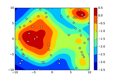
(b) Reference points on time stamp 2.

Figure 2. An example of ST reference points (shown as dots) on two different time stamps. The colorbars show the distribution of the ST field on the two time stamps.

3.2.4. Raster Data

In raster data, measurements of a continuous or discrete ST field are recorded at fixed locations in space and at fixed points in time. This is in contrast to point reference data where the ST reference sites may keep changing their location over time and collect recordings on different time stamps. To formally describe a raster, consider a set of fixed locations, $\mathcal{S}=\{s_{1},s_{2},\ldots,s_{m}\}$, either distributed regularly in space with constant distance between adjacent locations, e.g., pixels in an image (see Figure 3(a)) or distributed in an irregular spatial pattern, e.g., ground-based sensor networks (see Figure 3(b)). For every location, we record observations on a fixed set of time stamps, $\mathcal{T}=\{t_{1},t_{2},\ldots,t_{n}\}$, which can again be regularly spaced with equal delays between consecutive measurements (see Figure 3(c)) or irregularly spaced (see Figure 3(d)). It is the Cartesian product of $\mathcal{S}$ and $\mathcal{T}$ that results in the complete spatio-temporal grid, $\mathcal{S}\times\mathcal{T}$, where every vertex on the ST grid, $(s_{i},t_{j})$, has a distinct measurement.

(a) Regular space.

(b) Irregular space.

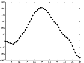
(c) Regular time.

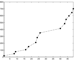
(d) Irregular time.

Figure 3. Different aspects of ST grids used for representing a raster data. The set of locations in the ST raster can either be located regularly or irregularly in space. The set of time stamps can also be either spaced regularly or irregularly.

ST raster data is quite common in several real-world applications such as remote sensing, climate science, brain imaging, epidemiology, and demography. Some examples of ST raster data include measurements collected by ground-based sensors of ST fields such as air quality or weather information, geo-registered images of the Earth’s surface collected by satellites at regular revisit times, and fMRI video sequences of brain activity. Note that while some examples of ST raster record observations at point vertices (e.g., measurements collected by a sensor network), others make aggregate measurements over the region at every grid cell. For example, demographic information is often collected at aggregate scales over political divisions such as cities, counties, districts, and states at annual scale. Another feature of an ST raster data is the resolution of the grid (both in space and in time) used for collecting measurements. In many applications, one commonly encounters ST raster data sets at varying resolutions of space and time, collected from different instruments or sensors. For example, satellite measurements of Earth’s surface may be obtained via Landsat instruments at 30 meter spatial resolution every 16 days or via MODIS instruments at 500 meter spatial resolution on a daily scale. As another example, fMRI technology can be used to measure brain activity at each 1mm x 1mm x 1mm location, whereas EEG technology measures activity at a selected set of tens of locations. In problems involving ST rasters with varying resolutions, we often need to convert an ST raster from its native resolution to a finer or coarser resolution, so that a seamless analysis of all ST rasters can be performed at a common resolution. Interpolation techniques, also referred to as resampling methods in Geographic Information System (GIS) literature, are commonly used to convert a raster data to a finer resolution in space or time. Note that the computational requirements of STDM methods generally increase as we move to finer resolutions in space and time. A raster data can also be converted to a coarser resolution by aggregating over collections of ST cells. Aggregation generally helps in removing redundancies in the observations, especially when there is high spatial and temporal auto-correlation at finer resolutions. However, it is important to keep in mind that aggressive aggregation of data to coarser resolutions may result in loss of information about the ST field being measured.

3.2.5. Converting Data Types

Even if an ST data is naturally collected in a particular data type in a certain application, it is possible to transform it to a different ST type so that the relevant family of STDM tools are used for their analyses. We provide some examples of inter-conversion among ST data types in the following. An event data type can be converted to a raster data type by aggregating the counts of events at every cell of an ST grid. For example, crime events can be counted at the levels of counties in a city at an hourly scale, thus producing an ST raster of crime occurrences. In some cases, a raster data can also be converted to ST events by using special algorithms for event extraction, e.g., techniques to find ST regions with abnormal activity. As an example, ecosystem disturbance events such as forest fires can be extracted from geo-registered satellite images of vegetation cover (Mithal et al., 2011a). Another common type of conversion among ST data types is between point reference data and raster data. Observations at ST reference points can be transformed into an ST raster format by interpolating or aggregating over an ST grid. Raster data can also be converted to a point reference data where every vertex of the ST grid is viewed as an ST reference point.

3.3. Data Instances

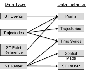
Figure 4. A mapping showing the different categories of ST data instances that can be constructed from ST data types.

The basic unit of data that a data mining algorithm operates upon is called a data instance. In classical data mining settings, a data instance is unambiguously represented as a set of observed features with optional supervised labels. However, in the context of ST data, there are multiple ways of defining instances for a given data type, each resulting in a different STDM formulation. In this section, we review five common categories of ST instances that one encounters in STDM problems, namely, points, trajectories, time series, spatial maps, and ST rasters. These data instances form the canonical building blocks of analysis for a broad range of problems and methods in STDM that we will discuss in Section 4.

Figure 4 summarizes the different types of data instances that can be constructed for each ST data type. While ST events can be naturally represented as point instances, a trajectory data type can either be represented as a collection of point instances (ordered list of locations visited by the moving object), a trajectory instance, or as a time-series of spatial identifiers (e.g., location coordinates). A ST reference data type comprises of point instances, where every instance is a reference point of the ST field in space and time. There are three different ways of constructing instances for ST raster data. First, we can define an instance to be the set of measurements at any location, $s_{i}$, represented as a time series, $T_{i}$. Second, we can also define an instance to be the set of measurements at any time stamp, $t_{j}$, represented as a spatial map, $S_{j}$. A third approach is to consider the entire ST raster (collection of observations over the entire ST grid) as a single data instance. It is the plurality of ways for defining instances for every ST data types that results in multiple STDM problems and methods. The choice of the right approach for constructing ST instances from a ST data type depends on the nature of the question being investigated, and the family of available STDM methods that can be used.

In the following, we introduce the five categories of ST data instances and discuss some of the common questions that can be investigated for each category. Since ST data instances can be summarized using a number of ways that go beyond standard dimensionality reduction techniques such as principal component analysis, we also describe some of the common ways of representing and summarizing the features for every instance category.

3.3.1. Points

An ST point can be represented as a tuple containing the spatial and temporal information of a discrete observation, as well as any additional variables associated with the observation. ST points are frequently used as data instances in STDM analyses involving event data, e.g., point events such as the occurrence of crimes at certain locations and times can be treated as basic instances to group similar instances or to find anomalous instances. ST points are also used as data instances when dealing with point reference data, where the measurements at ST reference points are used as instances to estimate the ST field at unseen instances. Additionally, a trajectory can also be viewed as an ordered collection of ST points, which are the locations visited by the moving object.

Some of the common questions that can be asked using ST points as data instances include: how are ST points clustered in space and time? What are the frequently occurring patterns of ST points? Can we identify ST points that do not follow the general behavior of other ST points? Can we estimate a target variable of interest at an ST point that has not been seen during training?

A collection of ST points can be summarized by measures that capture the strength of interaction (or auto-correlation) among the points. For example, the Ripley’s $K$ function (Dixon, 2002) is a commonly used statistic for describing the amount of attraction or repulsion among spatial locations beyond its expected value. Spatio-temporal extensions of the Ripley’s $K$ function have also been explored to measure the strength of interaction among ST point events (Lynch and Moorcroft, 2008). The strength of auto-correlation among ST reference points can also be measured using the Moran’s I function (Li et al., 2007a), local Moran’s I (Anselin, 1995), and its ST extension (Hardisty and Klippel, 2010).

3.3.2. Trajectories

Trajectories are a different class of data instances that can be used in STDM analyses involving moving bodies. Trajectories can be represented as multi-dimensional sequences that contain a temporally ordered list of locations visited by the moving object, along with any other information recorded by the object.

Some of the common questions that can be asked using trajectories as data instances include: can we cluster a collection of trajectories into a small set of representative groups? Are there frequent sequences of locations within the trajectories that are traversed by multiple moving bodies?

A common approach for representing and extracting features from trajectories is by the use of generative models (Gaffney and Smyth, 1999), where a parametric model is used to approximate the behavior of every trajectory. The learned parameters can then used as succinct representations of the trajectories. A trajectory can also be represented using the frequent sub-sequences of locations that are visited by the moving body. Techniques for identifying frequent trajectory patterns are discussed in detail later in Section 4.3.3. Distributed and efficient indexing structures for answering trajectory-related similarity queries have been developed in (Zeinalipour-Yazti et al., 2006; Al-Naymat et al., 2007). Apart from these methods, different schemes such as semantic trajectories (Bogorny et al., 2014; Li, 2017), symbolic trajectories (Güting et al., 2015), and spatio-textual trajectories (Damiani, 2016) are also recently being explored for representing trajectory data.

3.3.3. Time Series

Time series can be used as data instances in two different scenarios involving ST data. First, given an ST raster data, we can consider the set of observations at every spatial cell in the ST grid as a time series that can be used as a data instance in an STDM analysis. Second, a trajectory data can also be treated as a multi-dimensional time-series data, where the multiple dimensions correspond to the spatial identifiers (e.g., location coordinates) traversed by the moving objects over time, and any other variables recorded by the moving object in the course of its trajectory. While representing spatial identifiers as multiple (and independent) dimensions of a time-series may not preserve the spatial context among the identifiers, it opens up the vast literature on time series data mining that can be used for analyzing trajectories in novel ways, as will be described in Section 4.

Some of the common questions that can be asked using time series as data instances include: can we identify groups of time-series that show similar temporal activity and are located nearby in space? Are there some temporal patterns that commonly repeat in a number of time-series? Can we identify time stamps where the time-series deviate from their normal behavior for a short period of time? Can we discover time stamps where the time-series show a change in its profile? Can we use time-series as input features to predict a target variable? Can we predict the value of a time-series at a future time stamp using its historical values? Can we find distant groups of spatially contiguous time-series that are related to each other?

A number of approaches exist for extracting useful features from a collection of time-series. This include methods that can identify temporally frequent sub-sequences that occur in a majority of time-series (e.g., temporal motifs (Mueen, 2014)) or contain discriminatory information about a particular time-series class (e.g., shapelets (Ye and Keogh, 2009; Hills et al., 2014)). A review of techniques for identifying such frequent patterns in time-series is presented in (Fu, 2011) and (Esling and Agon, 2012).

3.3.4. Spatial Maps

An ST raster data can be viewed as a collection of spatial maps observed at every time stamp, which can also be used as data instance in analyses involving ST rasters.

Some of the common questions that can be asked using spatial maps as data instances in STDM analyses include: can we cluster the spatial maps to find groups of time stamps showing similar spatial activity? Can we identify spatial patterns that are observed in a number of spatial maps? Can we use spatial maps as input variables to predict a target variable? Can we predict the value at a certain location using observed values at other locations in the map?

A common approach for extracting features among spatial maps is using image segmentation techniques (Haralick and Shapiro, 1985). The presence or absence of different types of image segments can then be used as features to represent spatial maps.

3.3.5. ST Rasters

An ST raster data in its entirety, with measurements spanning the entire set of locations and time stamps, can also be treated as individual data instances in STDM analyses.

Some of the common questions that can be asked using ST rasters as data instances include: can we cluster ST rasters into groups that show similar behavior in space and time? Can we find frequent spatio-temporal behavior that occurs in a number of ST raster data sets? Can we find ST rasters that show distinctly different behavior than other ST rasters? Can we find timestamps where the behavior of an ST raster changes over time? Can we use ST rasters as input features for predicting a target variable of interest? Can we predict the value at a certain location and time stamp in the ST grid using observed values at other locations and time stamps? Can we find subsets of locations in the ST grid that show interesting relationships in their temporal activity?

A basic approach for representing ST rasters is using $N$-way arrays also called as tensors. In a tensor representation of an ST raster data, some dimensions are used to represent the set of locations while the remaining dimension is used to represent the set of time stamps available in the ST grid. For example, precipitation data is represented as a 3-dimensional array where the first two dimensions capture $2D$ space and the third dimension captures time. Similarly, fMRI data is represented as a 4-dimensional array where the first three dimensions capture $3D$ space and the third dimension captures time. A tensor representation of an ST raster data can then be summarized using space-time subspaces that have similar values, which are the equivalent of image segmentation in ST domains. Existing image segmentation techniques that have been extended to work with videos to discover moving objects are relevant to address this problem (Haritaoglu et al., 2000; Prati et al., 2003).

One way to summarize or extract features from ST rasters is by using network-based representations, where the nodes correspond to the locations and the edges denote the similarity among the time-series at locations (Atluri et al., 2016; Feldhoff et al., 2015). Techniques for computing similarity among time-series are discussed in detail later in Section 3.4.3. The topological properties of nodes such as degree and different variants of centrality measures can then be used to characterize the ‘role’ and ‘influence’ of locations. Such properties have been found to be useful in characterizing nodes in different types of networks such as social, biological, and transportation networks. For example, the use of network-based properties such as coherence among a set of locations (De Martino et al., 2007; Sui et al., 2009) or relationship between distant locations (Lynall et al., 2010; Pettersson-Yeo et al., 2011) has been explored in previous studies.

3.4. Similarity Among Instances

Determining similarity (or dissimilarity) between data instances is key to many data mining problems such as clustering, classification, pattern discovery, and relationship mining. Similarity measures have been extensively studied for data instances in traditional data mining settings, that are able to deal with varying types and formats of attributes. However, in the presence of space and time, there is a variety of ways we can define similarity among ST data instances such as points, trajectories, time-series, spatial maps, and ST rasters. Our ability to capture similarities among ST data instances using proximity measures underpins the effectiveness of STDM methods that build upon them. In the following, we describe some of the common ways for computing similarity among different types of ST data instances.

3.4.1. Point Similarity

Two points are considered close if they lie within the ST neighborhoods of each other. The ST neighborhood of a point can be defined using a fixed distance threshold in space and time, e.g., within 1 km radius and 1 hour time difference. Alternatively, the ST neighborhood of every point can also be defined in terms of a fixed number, $k$, of closest points. The choice of the right notion of locality depends on the application context and can be decided by the domain analyst.

3.4.2. Trajectory Similarity

Similarity among trajectories is often measured in terms of the co-location frequency, which is the number of times two moving bodies appear spatially close to one another. Other approaches for measuring similarity among trajectories include subsequence similarity metrics such as the length of the longest common subsequence, Fréchet distance, dynamic time warping (DTW), and edit distance (Toohey and Duckham, 2015). Trajectory similarity can also be computed using feature-based representations such as the frequent trajectory patterns extracted from the data.

3.4.3. Time Series Similarity

If we consider every time-series as a 1D-array of observations, the similarity among two time-series can be simply computed using proximity measures such as the Euclidean distance and the correlation strength, that consider a one-to-one correspondence between the elements of the two arrays. However, sometimes it is the case that two similar time-series are not exactly aligned with one another but show the same pattern of activity over time. Measures such as dynamic time warning (DTW) (Keogh and Ratanamahatana, 2005) and Fréchet distance (Alt and Godau, 1995) are able to capture such forms of similarity among time-series. We can also compute the similarity among two time-series based on their closeness in time-series features such as temporal motifs and shapelets. When it is expected to observe a certain delay or time lag between the observations of two time series, a common approach is to translate one of the time series with a range of candidate values of time lag and then choose the time lag that provides maximum similarity (e.g., highest absolute correlation).

While most measures of time-series similarity consider the entire time duration into account, it is possible that the similarity structure among time-series is subject to variation over time. For example, when a subject’s mental activity is switching between planning their day (i.e., an executive task) and reminding themselves of a recent meeting (i.e., a memory task), the similarity structure among the time-series at brain regions could be different. In such cases, a desired pattern of similarity among time-series may only be exhibited for short periods of time, which need to be determined from the data. An example of an approach that simultaneously identifies the relevant time windows for computing time-series similarity and uses this metric to cluster the time-series can be found in (Atluri et al., 2014).

3.4.4. Spatial Map Similarity

Two spatial maps can be considered similar if they show similar values at corresponding locations, which can be captured using standard proximity measures such as Euclidean distance. However, spatial maps can often suffer from small misalignments due to geo-registration errors, which can result in misleading distance metrics. Further, it is often more useful to compute similarity over smaller sub-regions in the map that contain foreground objects than considering the similarity over the entire map. The Earth’s mover distance (EMD) (Rubner et al., 2000) is one such metric that is robust to changes in the alignment of images, which is based on the minimal cost that must be paid to transform one image into the other. Spatial map similarity can also be computed on the basis of features such as image segments extracted from the data.

3.4.5. ST Raster Similarity

Network-based representations of ST rasters can be used to assess if two rasters are similar or not. For example, link and node similarity scores (Berg and Lässig, 2006; Li and Yang, 2009) can be used to compute the similarity among the corresponding links and nodes of ST rasters. ST raster similarity can also be computed on the basis of features extracted from their network representations (Soundarajan et al., 2013).

4. Problems and Methods

4.1. Clustering

Clustering refers to the grouping of instances in a data set that share similar feature values. When clustering ST data, novel challenges arise due to the spatial and temporal aspects of different types of ST instances. For example, clustering locations based on their time series of observations in an ST raster data has to ensure that the discovered clusters are spatially contiguous. Ignoring this spatial information can lead to fragmented clusters of locations that are difficult to interpret and have salt-and-pepper errors. Since many clustering algorithms use similarity measures for identifying groups of similar instances, techniques for computing similarity among ST instances (described in Section 3.4) will come in handy while clustering ST data. In the following, we describe some of the common methods for clustering different types of ST data instances.

4.1.1. Clustering Points

There are two different objectives that are of interest when clustering ST points. One objective involves finding clusters that have an unusually high density of ST points, also termed as hot-spots. This can be used for finding outbreaks of diseases or social movements, where there is a dense conglomeration of events both in space and time (Gomide et al., 2011; Kulldorff et al., 2005). This problem is also referred to as ‘event detection’ in the literature on mining social media data (Feng et al., 2015). The problem of finding hot-spots has been studied in the spatial statistics literature using methods such as the spatial scan statistic (Kulldorff, 1997), which explores all possible circular shaped regions of different sizes to determine regions where the incidence of points is significantly higher than expected. Generalization of the scan statistic for ST data, termed as space-time scan statistics, have been explored for studying disease outbreaks, crime hot-spots, and events in twitter data (Kulldorff, 2001; Kulldorff et al., 2005; Cheng and Wicks, 2014). While these early works provide a promising framework, open questions pertaining to shapes of regions (Takahashi et al., 2008; Eftelioglu et al., 2016), background distribution (Tango et al., 2011), and speed of search (Agarwal et al., 2006) are being investigated. Approaches for clustering spatial objects such as CLARANS (Ng and Han, 2002) can also be extended in the ST domain for finding groups of objects that are related in both space and time.

The second objective involves finding clusters of ST points that also have similar non-ST attributes. For example, given a collection of crime events, we may be interested in finding regions in space and time with similar crime activities. This clustering objective has been studied in the context of crime data (Eftelioglu et al., 2014), twitter data (Abdelhaq et al., 2013; Chierichetti et al., 2014; Ihler et al., 2006; Walther and Kaisser, 2013; Weng and Lee, 2011), geo-tagged photos (Zheng et al., 2012), traffic accidents (Zheng et al., 2012), and epidemiological data (Glatman-Freedman et al., 2016). A number of techniques for clustering ST points are based on the DBSCAN algorithm (Ester et al., 1996), which is a widely used method for finding arbitrarily shaped clusters of spatial points based on the density of points. ST-DBSCAN (Birant and Kut, 2007) is one of the popular extensions of DBSCAN that defines two separate distances between ST points: one that captures spatial attributes and another that captures temporal and non-ST attributes. Computing distance based on spatial, temporal and non-ST attributes separately and having separate thresholds for them provides the user a flexibility to determine the desired spatial density that is relevant to the problem at hand. However, several challenges including heterogeneity in space and time, varying densities of clusters, and sampling bias inherent in the data are yet to be addressed.

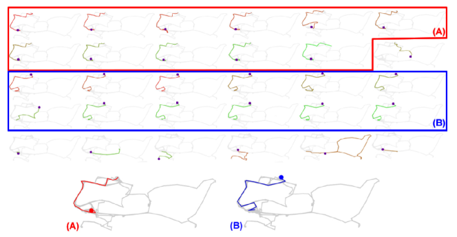
Figure 5. Mobility profiles discoverd from a user’s GPS traces based on clustering of trips. (Figure taken from (Trasarti et al., 2011))

4.1.2. Clustering Trajectories

When clustering trajectory data, we are often interested in finding groups of trajectories that are similar to each other across the entire duration of trajectories. For example, clustering of trajectories has been used to find groups of hurricanes with similar trajectories (Lee et al., 2007), groups of taxi traces that follow a similar route (Liu et al., 2010), or groups of moving objects that follow the same motion in video streams (Gaffney and Smyth, 1999). A review of techniques for clustering trajectories is presented in (Kisilevich et al., 2010). Two important aspects of trajectory clustering methods are the choice of distance measure (see Section 3.4.2) and the choice of clustering technique (Morris and Trivedi, 2009). One category of methods for clustering trajectories involves using mixture modeling approaches (Gaffney and Smyth, 1999; Chudova et al., 2003; Alon et al., 2003), e.g., mixtures of regression models where a different regression model is learned for every cluster of trajectories (Gaffney and Smyth, 1999). A different approach has been explored in (Trasarti et al., 2011), where a two-step clustering method was proposed to find mobility profiles of users based on their GPS traces. Figure 5 shows two sets of discovered profiles (A and B), along with several noisy trips that do not conform to these profiles.

In some trajectory clustering problems, we are interested in finding groups of trajectories that share similarity in only a short duration of the trajectory. One of the methods developed for this problem is a partition-and-group framework called TRACLUS (Lee et al., 2007), which first partitions each trajectory into smaller line segments based on a minimum description length (MDL) principle, and then groups line segments based on their similarity using a DBSCAN-based approach.

A related area of research is the identification of “moving clusters” of trajectories, where moving bodies may join or leave a cluster as it progresses in space over time. This is a common pattern that is observed in several applications, e.g., migrating flocks of animals or convoys of cars. Algorithms for detecting moving clusters of trajectories have been developed in (Kalnis et al., 2005) and in subsequent studies (Jeung et al., 2008; Li et al., 2010; Dodge et al., 2008). More recently, (Zhang et al., 2016) proposed an iterative framework, GMove, that alternates between two tasks: assigning users to groups and modeling group-level mobility, using an ensemble of hidden Markov models.

4.1.3. Clustering Time Series

A central objective when clustering time series derived from ST raster data (using the series of measurements at every location) is to find spatially coherent groups of locations with similar temporal activity. This problem has been approached from multiple directions. One direction is to use traditional clustering schemes such as $k$-means clustering (Mezer et al., 2009), hierarchical clustering (Goutte et al., 1999), shared nearest neighbor (SNN) clustering (Steinbach et al., 2003), and normalized-cut spectral clustering (Van Den Heuvel et al., 2008) to cluster time series (using the time series similarity measures discussed in Section 3.4.3). The clustering of Sea Level Pressure time series, studied in climate science, from all locations on the Earth’s surface is shown in Figure 6. Data from 1982 to 1993 was used to find these clusters and Pearson’s correlation coefficient was used to assess similarity between time series.

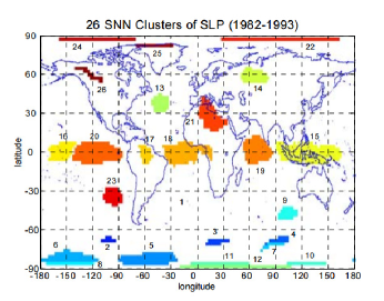
Figure 6. Clusters found using SNN clustering of Sea Level Pressure data (1982-1993). (Figure taken from (Steinbach et al., 2002))

Since traditional approaches for time series clustering do not guarantee that the resultant clusters are spatially contiguous, this is typically addressed in a post-processing step either by increasing the number of clusters  (Smith et al., 2009) or by separating clusters with non-contiguous sets into multiple contiguous clusters. Another direction is to directly incorporate spatial contiguity in the clustering process, e.g., by using ‘region growing’ approaches or by enforcing contiguity constraints in the clustering technique. Region growing approaches (Heller et al., 2006; Lu et al., 2003b; Bellec et al., 2006) work by merging spatially adjacent locations that are highly similar to each other (defined using similarity measures discussed in Section 3.4.3) into a single cluster until a minimum number of clusters has been achieved or no cluster can be further grown without violating a similarity criterion. While region growing approaches ensure that every cluster has similar locations, they do not ensure that the different clusters are dissimilar. On the other hand, clustering approaches that utilize contiguity constraints (Craddock et al., 2012; Blumensath et al., 2013) do not have this problem as these approaches ensure that locations within a cluster are highly similar to each other than locations that are in two different clusters.

4.1.4. Clustering Spatial Maps

When clustering spatial maps (sets of measurements from all locations in an ST raster on different times), the central objective is to find groups of time stamps that have similar spatial maps, e.g., time stamps with similar maps of brain activity (Liu and Duyn, 2013). Similarity measures among spatial maps, such as those discussed in Section 3.4.4, can help in discovering meaningful clusters of spatial maps irrespective of data artifacts such as changes in alignment and registration among the locations of different maps (Liu et al., 2013). While these methods are useful in producing temporally contiguous segments with similar spatial activity (due to the temporal auto-correlation in the data), in some cases, we may be interested in identifying non-contiguous groups of time stamps. One way to ensure that a given cluster of spatial maps is not due to temporal auto-correlation is to evaluate this in a post-processing step or use a smaller $k$ such that distant time points are grouped into clusters.

4.1.5. Finding Dynamic ST Clusters

A common clustering problem that is of interest when dealing with ST raster data is to identify sub-regions of space and time that show coherent measurements, termed as ‘dynamic ST clusters’ (Chen et al., 2015). The discovery of dynamic ST clusters can help in detecting phenomena that only influence a subset of locations during a subset of time points. For example, water bodies that grow and shrink in space over time, e.g., lakes and reservoirs, can be identified as dynamic ST clusters in remote sensing data, as they appear as coherent observations in subsets of space and time. Note that a dynamic ST cluster may evolve over time and thus change its shape, size, and appearance as we progress in time. Hence, while some locations are retained across consecutive time stamps, the cluster assignments of locations are dynamic and the clusters can grow and shrink over time. A recent work (Chen et al., 2015) explored a novel approach to identify dynamic ST clusters in raster data sets for detecting surface water dynamics, which used an iterative algorithm to first identify the set of ‘core’ locations that are part of a dynamic cluster across all time stamps, and then growing around the core locations at every time stamps to capture the dynamic behavior occurring at the boundaries. Similar formulations can be developed for identifying other types of dynamic clusters in ST raster data, e.g., a moving cluster of locations such as the evolution of a hurricane.

4.1.6. Clustering ST Rasters

Given a collection of ST raster data sets, possibly collected over different spatial regions and time periods, it is useful to identify groups of ST raster data sets considered as individual instances. This has applications in several domains dealing with ST raster data such as climate science and neuroimaging. For example, in climate science, different climate models produce simulations of global climate variables as ST rasters, which when clustered sheds light on the similarity of climate models (Steinhaeuser and Tsonis, 2014). ST rasters can be clustered by using similarity measures among ST rasters as basic building blocks, which typically involve extracting features from network representations of ST rasters (discussed in Section 3.4.5). For example, (Yu et al., 2015b) found groups of ST rasters by first constructing networks from ST rasters and then grouping the resultant networks using a network module-finding approach from (Newman, 2006). However, extracting such high higher-order features from ST rasters is non-trivial and often requires domain expertise.

4.2. Predictive Learning

The basic objective of predictive learning methods is to learn a mapping from the input features (also called as independent variables) to the output variables (also called as dependent variables) using a representative training set. In spatio-temporal applications, both the input and output variables can belong to different types of ST data instances, thus resulting in a variety of predictive learning problem formulations. In the following, we discuss some of the predictive learning problems that are commonly encountered in ST applications based on the type of ST data instance used as input variables.

4.2.1. Time Series

Given an ST raster data, we can consider the problem of predicting an output variable (continuous or categorical) at every location of the raster using the time-series at every location as input variables. The use of time-series as input features is quite common in a number of classification and regression problems. For example, the temporal dynamics of audio frequencies is used to classify words or sentences in human speech recognition problems. This can be achieved by using recurrent neural networks (Mikolov et al., 2010; Graves and Schmidhuber, 2009), which are extensions of artificial neural networks with appropriate skip connections among the neural nodes to model information delay. Another approach to incorporate the temporal context of time-series features in classification problems is the use of shapelets (Ye and Keogh, 2009; Hills et al., 2014). Shapelets are time-series subsequences that are discriminative in nature, i.e. their occurrence is selective to certain classes. While these techniques provide an ability to model the temporal characteristics of input features, there is a need to develop novel methods that can take into account the spatial information among the time-series in ST rasters. For example, instead of predicting the class label at every location using its time-series independently, we can leverage information about spatial neighborhoods to enforce spatial consistence among the labels at nearby locations. Variants of recurrent neural networks that include spatial features for spatio-temporal prediction have been explored in (Jia et al., 2017b, a; Jain et al., 2016). Latent space models that use topological as well as temporal attributes of locations have also been developed for real-time traffic prediction using time-varying information from sensor recordings (Deng et al., 2016). Time series can also be constructed from trajectory data, where the objective is to predict the future location of a moving object (or a group of objects), given their past history of visited locations (Li et al., 2016; Horton et al., 2014).

4.2.2. Spatial Maps

In this class of predictive problems, a scalar output variable has to be predicted at a time-step of the ST raster, using the spatial map at the same time-step as input variables. Some examples of applications that use spatial maps as input features include image classification and object recognition problems, where a categorical value has to be assigned to every image or sub-region in an image using the information contained in spatial maps. A classification approach that has recently gained widespread recognition in the computer vision community is deep convolutional neural networks (CNN) (LeCun and Bengio, 1995; Krizhevsky et al., 2012), that use the spatial nature of inputs to share model parameters and provide robust generalization performance. In spatio-temporal applications, a promising research direction is to use the temporal auto-correlation among consecutive spatial maps to share the parameters of CNN models over time. Spatio-temporal extensions of CNN based learning frameworks have been developed in (Taylor et al., 2010; Karpathy et al., 2014). Extensions of neural networks that use both the spatial and temporal information of data have also been developed in (Stiles and Ghosh, 1997; Ghosh and Deuser, 1995), where the network design was inspired by the biological information of habituation mechanisms in neuroscience.

4.2.3. ST Rasters

Another class of predictive learning problems is to use the entire information in an ST raster as input variables to predict a scalar output variable. An example of this is to predict if a subject has a mental disorder or note based on their fMRI scan, stored as an ST raster. This has tremendous applications in diagnosing mental disorders which is currently done in a very subjective manner. Another application that is increasingly becoming popular in the realm of brain imaging is that of ‘brain reading’ (Norman et al., 2006), where the objective is to determine the nature of activity (e.g., planning, memorizing, recollecting etc.) based on measured spatio-temporal activity from the brain, represented as an ST raster.

A naïve approach to this problem could involve representing every ST raster with $|\mathcal{S}|$ locations and $|\mathcal{T}|$ time stamps as a vector of size $|\mathcal{S}|\times|\mathcal{T}|$, and employing traditional classification schemes on these vector representations, e.g., linear discriminant analysis and support vector machines (Ku et al., 2008). Note that this is only possible when the ST grid of every grid is perfectly aligned with each other, such that their sets of locations and time stamps are identical. This is not usually the case with resting state fMRI scans, because the time points in one subject’s scan cannot be matched with those of another subject. Furthermore, especially in fMRI data, the large number of spatial locations (typically hundreds of thousands) and time points (typically hundreds) leads to millions of potential features, where the number of instances are often tens to hundreds, leading to the phenomena of model overfitting. Hence, it is important to use derived features from ST rasters that summarize the ST activity of every raster, as described in Section 3.3.5. Alternatively, tensor learning based approaches (Zhou et al., 2013a; Bahadori et al., 2014; Yu et al., 2015a) provide a way to reduce the model complexity by making use of the spatial and temporal dependencies among the input features, thus showing a promise in predictive learning problems involving input ST rasters.

4.2.4. ST Reference Points

A common predictive learning problem in spatio-temporal applications is to predict the response at a certain location and time using observations collected at other locations and time stamps (often in ST neighborhoods). This is important in a number of domains, e.g., while estimating an ecological variable over every location and time using remote sensing observations at nearby locations and time stamps. The problem of land cover classification (estimating a categorical label at every location and time indicating its propensity to belong to a land cover type) has been heavily studied in the remote sensing literature for a variety of problems (DeFries and Chan, 2000; Vatsavai, 2008; Jun and Ghosh, 2011; Li et al., 2014b), e.g., the mapping of surface water dynamics using multi-spectral remote sensing data (Khandelwal et al., 2017; Karpatne et al., 2016b). As another example, the outbreak of influenza at a given location and time can be predicted based on web searches (Ginsberg et al., 2009) and twitter messages (Culotta, 2010) at neighboring locations and times. There are two classes of methods that are relevant for making predictions at ST reference points: methods that use the temporal information to predict values at nearby time points, and methods that use the spatial information to estimate values at nearby spatial points. We discuss both these classes of methods in the following.

Using Temporal Information:

In many domains such as climate and health, estimation (or forecasting) of the future conditions based on present and past conditions is desired. For example, the sea surface pressure and temperature for the present month can be predicted based on values in the previous months. Similar problems are studied in predicting closing stock prices at the New York Stock Exchange and in predicting sales in the manufacturing industry (Montgomery et al., 2015). Some of the widely used methods for time-series forecasting problems include exponential smoothing techniques (Gardner, 2006), ARIMA models (Box and Jenkins, 1976), and state-space models (Aoki, 2013). Another type of methods for making predictions at time stamps include dynamic Bayesian networks such as hidden Markov models and Kalman filters (Rabiner and Juang, 1986; Harvey, 1990), that estimate the most likely sequence of latent values at time stamps using the temporal auto-correlation structure. Techniques that make predictions in time need to be modified to include the spatial context in spatio-temporal applications. As an example spatio-temporal Granger causality models, that use both spatial and temporal information in the regression models, have been explored to model relationships among ST variables (Lozano et al., 2009b; Luo et al., 2013).

Using Spatial Information:

There is a vast body of literature on spatial prediction methods that take into account the spatial auto-correlation structure in the data to ensure spatially coherent results. This includes the use of spatial auto-regressive (SAR) models (Kelejian and Prucha, 1999), geographically weighted regression (GWR) models (Brunsdon et al., 1998), and Kriging (Oliver and Webster, 1990) in the spatial statistics literature. Markov random field based approaches that are naturally suited to handle the spatial auto-correlation in the data have also been widely studied (Kasetkasem and Varshney, 2002; Schroder et al., 1998; Zhao et al., 2007). There is a promise in informing such techniques with the temporal nature of ST points in spatio-temporal applications, such that both spatial and temporal auto-correlation are incorporated in the modeling framework. For example, spatio-temporal Kriging approaches have been used in a number of applications in climate and environmental modeling (Cressie and Wikle, 2015), where time is treated as another dimension while learning covariance structures in space and time. A related area of research is spatial item recommendation (Wang et al., 2017), where the preference over spatial items (e.g., restaurants or tourist attractions) have to be predicted in a time-varying manner, using social network information and the history of preferences of every user.

4.3. Frequent Pattern Mining

Frequent pattern mining is the process of discovering patterns in a data set that occur frequently over multiple instances in a data set, e.g., frequently bought groups of items in market-basket transactions. Given the rich variety of data types and instances in ST applications, there are several categories of frequent pattern mining problems that can be formulated in the presence of spatial and temporal components, as described in the following.

4.3.1. Co-occurrence Patterns in ST Points

Given a collection of points such as ST events of varying types, a common pattern of interest is co-occurrence patterns, which are basically subsets of ST event types that occur in close spatial and temporal proximity of each other. For example, given a data set of crime and other events in a city, we may be interested in finding ST event types that occur together (e.g., bar closing and drunk driving). Co-occurrence patterns has been studied in the context of spatial datasets as ‘co-location’ patterns for more than a decade (Huang et al., 2004; Xiao et al., 2008; Wang et al., 2013). In the spatial statistics literature, co-locations have been studied using measures such as the Ripley’s cross-$K$ function (Dixon, 2002), which capture statistical patterns of attraction or repulsion among pairs of spatial point types.

One of the first approaches for discovering co-occurrence patterns include an Apriori-principle based approach developed by (Pillai et al., 2012). This approach relies on an interestingness measured termed as spatio-temporal co-occurrence co-efficient to capture co-occurrence in spatial and temporal dimensions. A filter and refine approach was later proposed in (Pillai et al., 2013) to tackle the problem of discovering co-occurrence patterns in large event databases. Constructing rules from co-occurrence patterns have also been studied in (Pillai et al., 2014). Spatio-temporal extensions of the cross-$K$ function have been proposed in (Lynch and Moorcroft, 2008), where the ST neighborhood of ST points is used for identifying attraction or repulsion patterns among ST point types in both space and time.

4.3.2. Sequential Patterns in ST Points

Sequential patterns have been studied in the context of ST event data, where the occurrence of ST events of a particular type can trigger a sequence of ST events of other types. For example, a car accident on a freeway could trigger a traffic jam in its ST neighborhood. Sequential patterns have been originally defined in the context of market-basket transactions where sequences of transactions from every customer are available and the goal is to discover ordered list of items appearing with high frequency (Agrawal and Srikant, 1995). An approach for discovering sequential patterns of ST event types was presented in (Huang et al., 2008). This approach was able to discover ordered lists of event types such as $f_{1}\rightarrow f_{2}\rightarrow\ldots\rightarrow f_{n}$, where events belonging to type $f_{1}$ trigger events of type $f_{2}$, that further triggers events of type $f_{3}$ and a series of events resulting in events of type $f_{k}$. They developed an Slicing-STS-Miner approach to efficiently discover statistically significant sequential patterns of events. A partially-ordered subsets of event types, referred to as cascading spatial temporal patterns (Mohan et al., 2012, 2010), have also been studied to capture event sequences whose instance are located together and occur in successive stages. Some of the key challenges in mining ST sequential patterns include defining interesting measures that capture meaningful non-spurious patterns and developing efficient approaches to discover interesting patterns from an exponentially large space of candidate patterns.

4.3.3. Sequential Patterns in Trajectories

Sequential patterns in trajectories are sequences of spatial locations or regions that are visited by multiple moving objects in the same order, and are thus covered by multiple trajectory instances. For example, given the trajectories of tourists visiting a city, we can find sequential patterns that represent the typical behavior of tourists as they visit an attraction and move to another. Although trajectories can be treated as multi-dimensional sequences where the spatial identifiers (e.g., latitude and longitude) of visited locations are used as dimensions, traditional sequential pattern mining approaches are unsuitable for finding sequential patterns of trajectories because of their inability to handle the spatial nature of information contained in trajectories. For example, the locations visited by moving objects may not exactly match but be in close spatial vicinity to be considered as part of the same pattern. Moreover, trajectories belonging to a common sequential pattern are expected to follow similar spatial path but not exactly the same path. To handle the spatial aspect of trajectories in the process of mining sequential patterns, (Tsoukatos and Gunopulos, 2001) used ordered sequences of spatial elements such as rectangular regions to define sequential patterns. A trajectory is then considered to be part of a sequential pattern if every line segment joining consecutive locations of the trajectory are enclosed within the rectangular regions of the pattern. A similar approach for sequential pattern mining was developed in (Cao et al., 2005) where pattern elements were defined as spatial regions around frequent line segments of trajectories. Spatio-temporal extensions of association rules, termed as spatio-temporal association rules (STARs) (Verhein and Chawla, 2006), have also been explored to find frequent patterns of geographic regions visited by moving objects (Verhein and Chawla, 2008). Approaches for mining periodic patterns in trajectories, where moving objects periodically visit sequences of locations in time, have been developed in (Li and Han, 2014). Approaches to handle uncertainty have also been studied to handle the incompleteness of the data and artificial noise introduced in privacy-sensitive applications (Chen et al., 2016; Li et al., 2013).

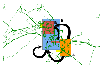
Figure 7. Example of a sequential patterns found in GPS traces of trucks in Athens, Greece. (Figure taken from (Giannotti et al., 2007))

Another aspect of trajectories that is important to consider while mining sequential patterns in some applications is the presence of timing constraints among visited locations. For example, we may be interested in finding sequential patterns where the time duration between consecutive locations are similar across the trajectory instances, in addition to the similarity of paths followed by the moving objects (Giannotti et al., 2007). This approach was used to discover sequential patterns in GPS traces of trucks in Athens, Greece. One resultant pattern A $\xrightarrow{\Delta t1}$ B^′ $\xrightarrow{\Delta t2}$ B^′′ is shown in Figure 7 that captures how the trucks visit region A first, then visit region B^′, and then visit region B^′′, with fixed time gaps between the locations. Another way of introducing timing constraints is to consider sequential patterns of trajectories that are in close temporal proximity of each other, i.e., the moving objects visit a sequence of locations at similar points in time. Such patterns are referred to as ‘flock patterns’ (Vieira et al., 2009) or ‘convoys’ (Jeung et al., 2008) that are used for finding groups of objects moving together.

4.3.4. Motif Patterns in Time-series

In the context of ST raster data, time-series motifs represent repeated temporal measurements observed across multiple spatial locations. For example, in vegetation time series data of agricultural farms, the harvesting cycles of crops can be discovered as time-series motifs that recur at multiple farm locations belonging to the same crop type. Time-series motifs have been extensively studied in applications such as ecology, medicine, finance, and production industry (Mueen, 2014; Torkamani and Lohweg, 2017). While the naïve approach for discovering motifs is quadratic in the length of the time series, approximate approaches (Chiu et al., 2003; Meng et al., 2008; Minnen et al., 2007) have also been designed. Recently, the development of efficient approaches for constructing ‘matrix profile’ (Yeh et al., 2016), a vector comprised of minimum non-trivial distance for each subsequence in time series $A$ with subsequences in time seies $B$, have enabled an efficient approach for motif discovery (Zhu et al., 2016). At the heart of this approach for computing the matrix profile is a fast Fourier transform based algorithm for efficiently computing z-normalized Euclidean distance between two time series subsequences. Using this approach, subsequence similarity in any given time series can be efficiently computed and the subsequences that are highly similar correspond to motifs.

While traditional formulations for motif discovery assume independence among the time-series, in ST applications, there is a strong spatial auto-correlation among the time-series at nearby locations, limiting the usefulness of existing formulations. This is because any time-series motif observed over a set of locations may also show up in the neighborhood of those locations with minor variations, resulting in a number of redundant patterns that look almost similar. One approach to address this challenge is to enforce motif discovery algorithms to identify recurring temporal patterns that appear synchronously in spatially coherent regions, in contrast to isolated points in space. This would result in the discovery of physically relevant processes and events that span both space and time, e.g., droughts or floods affecting an ST region in climate data sets. We can call such ST motifs as ‘spatially coherent time-series motifs.’ It may also be useful to explore a slightly modified version of this problem where locations belonging to the same region do not synchronously show a common pattern but instead there is a gradual evolution of temporal activity across them. Such ‘evolving ST motifs’ can help us detect frequent ST phenomena that gradually moves across locations in a region.

An active research direction is to discover structural patterns in ST data that elucidate complex spatial and temporal dynamics. For example, (Zhou and Matteson, 2015) developed approaches to discover ST dynamics in ambulance demand data for ambulance fleet management. A major challenge in this direction is to handle the heterogeneity in the presentation of different patterns in space and time. Sparsity of the underlying data also poses a challenge to capture patterns of interest. While early efforts in using tensor-based factorization (Takahashi et al., 2017), multi-task learning (Zhao et al., 2015), and spatio-temporal kernel density estimation (Zhou and Matteson, 2015) approaches have shown promise, their effectiveness in handling heterogeneity and sparsity is yet to be investigated.

4.3.5. Network Patterns in ST Rasters

Given a collection of ST rasters, we are interested in discovering patterns of structure in network-based representations of ST data (described in Section 3.3.5), which occur frequently in multiple ST rasters. A commonly studied type of network structure is the arrangement of communities in the network, where a community represents a group of entities (nodes or links) that interact among themselves more than they do with the rest of the entities (Leskovec et al., 2010). Another type of network structure is network motifs (Milo et al., 2002), which are the basic building blocks of the connectivity patterns that frequently occur across multiple network instances. The use of network motifs has been explored in several domains, e.g., bioinformatics (Shen-Orr et al., 2002) and social networks (Milo et al., 2002).

In ST applications, network motif discovery has been used to identify the inherent ST structures of brain fMRI data (Sporns and Kötter, 2004). Network communities in ST rasters can reveal interesting high-level patterns. For example, in climate data, a community can represent a set of distant locations that are experiencing similar climatic conditions and show consistent temporal activity. While the discovery of network patterns can prove to be a valuable tool in the analysis of ST raster data sets, care must be taken while using them as the spatial auto-correlation in the data can result in a number of spurious edges that can lead to misleading results. Hence, during the evaluation of patterns in network-based representations of ST rasters, it is important to filter out patterns arising from spatially neighboring locations for the discovery of long-range dependencies between distant locations.

4.4. Anomaly Detection

Anomalies are traditionally defined as instances that are remarkably different from the majority of instances in the data set. In ST applications, detecting anomalies (also referred to as outliers) can help us identify interesting but rare phenomena, e.g., an anomalous trajectory taken by a taxi vehicle or the changing frequencies of floods and droughts in certain areas due to climate change or human actions that change the ecology of a region. Given a method for computing pair-wise similarities among ST instances (discussed in Section 3.4), anomalies can be identified as instances that are highly dissimilar from the rest of the instances. Detecting anomalies can also be seen as a by-product of clustering, since instances that do not easily become part of a cluster or form an isolated cluster that is quite far from the other clusters can be termed as anomalies. There are two areas of work that are relevant in the context of detecting anomalies in ST data. First, a number of techniques have been developed for identifying anomalies in time series data, which are also called as discords. This includes approaches for univariate time series (Bishop, 1994; Keogh et al., 2002; Wei et al., 2005; Keogh et al., 2005) as well as multivariate time series (Chen et al., 2008; Galeano et al., 2006; Baragona and Battaglia, 2007; Takeishi and Yairi, 2014) A survey of anomaly detection approaches for temporal data is presented in (Gupta et al., 2014). Second, approaches for detecting anomalies in spatial data, also termed as spatial outliers, have also been developed (Shekhar and Chawla, 2003). Spatial outliers are defined as points whose non-spatial attributes are different from those that are in its close spatial neighborhood . Techniques for detecting spatial outliers vary in their choice of method for constructing local neighborhood and assigning anomaly scores, e.g., using spatial distance measures (Knorr and Ng, 1997; Knorr et al., 2000; Lu et al., 2003a), graphical-distance measures (Shekhar et al., 2001; Kou et al., 2007), and visualization tools such as the Moran’s I scatter plot, pocket plots, and the Variogram Cloud plot (Anselin, 1994; Haslett et al., 1991). A review of techniques for spatial outlier detection is presented in (Aggarwal, 2017). However, the joint presence of spatial and temporal aspects introduces novel ways of describing anomalies in ST data, resulting in unique anomaly detection problems, as described below.

4.4.1. ST Point Anomalies

The concept of spatial outliers can be easily extended to spatio-temporal domains, where the neighborhood of an ST point is defined with respect to both space and time. Thus, a spatio-temporal outlier is basically an ST point that breaks the natural ST auto-correlation structure of the normal points. One approach to find ST outliers is to first cluster the normal points using approaches such as ST-DBSCAN, and then report points that did not conform well to the discovered clusters (Kut and Birant, 2006). Another category of approaches presented in (Cheng and Li, 2004, 2006) is to aggregate ST clusters at a coarser scale so that the effect of outliers on the clustering is reduced. ST outliers are then detected by comparing the original clustering with the coarsened clustering. Note that most ST outlier detection algorithms assume homogeneity in neighborhood properties across space and time, which can be violated in the presence of ST heterogeneity. This can be handled by methods that model the variance of normal instances in the local neighborhood of every point, along with its expected value (Sun and Chawla, 2004).

4.4.2. Trajectory Anomalies

There are several ways we can identify a trajectory to be anomalous. A common approach is to compute pair-wise similarities among trajectories (discussed in Section 3.4.2) and identify trajectories that are spatially distant from the others. For example, (Lee et al., 2008) explored varying notions of distances between trajectory sub-sequences (such as perpendicular distance, parallel distance, and angle distance) and identified a trajectory to be anomalous if it had very few neighbors within a certain threshold. Distance based methods for detecting anomalous trajectories have also been explored in (Bu et al., 2009), where trajectories that appear in distant spatial regions than the rest of the trajectories are considered anomalous. Another class of approaches is to aggregate the spatial shapes of trajectories using a coarse spatial grid, and then compute useful characteristics of a trajectory in every spatial grid cell. For example, we can compute the average direction of trajectories in every spatial grid and identify a trajectory as anomalous if it deviates from the expected behavior in a number of grid cells that it covers, as proposed in (Ge et al., 2010). A graph-based approach for detecting outliers in traffic data streams was developed in (Liu et al., 2011), where nodes are regions and edge weights represent the traffic flow between regions. Traffic outliers were discovered as edge anomalies in this graph, which were subsequently analyzed for causal interactions using causal outlier trees. Supervised methods for detecting anomalous trajectory shapes (or motifs) have also been explored in (Li et al., 2006; Li et al., 2007b).

While the techniques discussed above for identifying trajectory anomalies focused on the spatial pattern (e.g., shape, distance, or angle) of trajectories, we can also consider a trajectory to be anomalous if it deviates from its local neighbors as it switches from one cohort to other, e.g., a zebra moving from one group to another. To identify such anomalies, the approach presented in (Li et al., 2009) computed the spatial neighbors of every moving object at any given time stamp (using trajectory information in the immediate history) and designed an anomaly score based on deviations from the trajectories of neighbors. Such an approach can enable the discovery of trajectories that are contextually anomalous in their local neighborhoods, and can thus be robust to aggregate changes such as population shifts. It can also be useful for detecting anomalies in an on-line fashion, as trajectories that begin to drift apart from their local neighbors will start to accumulate large anomaly scores in a short number of time stamps.

4.4.3. Group Anomalies in ST Rasters

While techniques described in Section 4.4.1 are well-suited for discovering ST point anomalies, it is often the case that anomalies appear in ST raster data as spatially contiguous groups of locations (regions) that show anomalous values consistently for a short duration of time stamps. Some examples of such group anomalies in ST raster data include rare events such as cyclones, floods, and droughts that result in abnormally high or low precipitation in a given region for a certain duration of time, or an abnormal number of tweets or emergency calls from a spatial region in a small time window.

Most approaches for detecting group anomalies in ST raster data decompose the anomaly detection problem by first treating the spatial and temporal properties of the outliers independently, which are then merged together in a post-processing step. For example, the approach presented in (Wu et al., 2010) made use of the spatial scan statistic to find the top-$k$ contiguous groups of locations that showed anomalous activity at every time stamp. These groups of locations were then stitched together in time to find ST groups of anomalous values. A similar line of work has been explored in (Lu et al., 2007), where the anomalous spatial regions were discovered using an image segmentation algorithm and a regression technique was applied to track the movement of the centers of the anomalous regions across consecutive time stamps. Another approach for detecting anomalies in ST raster data was explored in (Faghmous et al., 2013a) for discovering ocean eddies in climate data. Ocean eddies are revolving masses of water in the ocean that appear as local extremas (depressions or elevations) in a snapshot of sea surface height data on any given time stamp, and these extremas keep moving over time. The approach presented in (Faghmous et al., 2013a) identified eddies as local extremas in space using a bottom-up thresholding scheme, which could then be stitched in time using multiple hypothesis object tracking procedures (Faghmous et al., 2013b). An orthogonal approach to detecting anomalies in ST rasters is to find anomalies in time series data that can then be merged across space (Faghmous et al., 2012).

Approaches for detecting anomalies in ST raster that jointly use information about the spatial and temporal aspects of the data have also been developed. For example, in the application of detecting abnormal activities in crowded scenes from surveillance camera videos, anomaly detection approaches using models of normal activity have been developed in (Li et al., 2014a; Kratz and Nishino, 2009). In this problem, a major difficulty is to come up with a notion of normal motion activity that can be differentiated from anomalous activities, which can be quite complex in crowded atmospheres. To address this challenge, (Li et al., 2014a) used a mixture of dynamic textures models to capture the spatial and temporal salience of normal activities, borrowing from the vast literature on activity recognition in the area of computer vision. Spatial and temporal anomaly maps are then constructed at multiple spatial scales, which are then integrated together using a conditional random field framework. On the other hand, the approach presented in (Kratz and Nishino, 2009) model the steady-state motion behavior of normal space-time volumes that can capture the variations in the ST data and can compactly represent the overall video volume. These models are then used to detect unusual motion activities as statistical deviations from the normal model.

A special type of group anomaly in ST rasters is bursts of activity in the time series of locations, detected for short time periods. For example, Twitter queries involving specific terms such as ‘earthquake’ can be discovered as spatio-temporal burst events related to natural disasters. One of the early works on detecting ST burst events includes the work by (Lappas et al., 2012), where both the spatial and temporal nature of burst patterns were jointly taken into consideration. A system for mining ST burst events, termed as the Spatio-TEmporal Miner (STEM), has been developed in (Lappas et al., 2013).

4.5. Change Detection

The problem of change detection involves identifying the time point when the behavior of a system undergoes a significant deviation from its past behavior. Detecting changes in ST data is useful in several applications, e.g., discovering transitions from an El Nino phase to a La Nina phase in climate science (Miralles et al., 2014) or understanding the switching of the state of the brain from planning to cognition in brain imaging data (Tang et al., 2012).

Change detection has been extensively studied in the context of time-series data, where the objective is to determine time intervals (segments) that exhibit homogeneous properties (Keogh et al., 2004; Liu et al., 2008; Mithal et al., 2012; Huang et al., 2013). Different types of homogeneity in segments such as mean (Bernaola-Galván et al., 2001; Horváth, 2001), variance (Whitcher et al., 2000; Andreou and Ghysels, 2002; Inclan and Tiao, 1994), and distribution statistics (Carpena and Bernaola-Galván, 1999; Grosse et al., 2002) have been used for identifying time series segments and their changes. Apart from time series segmentation, other approaches has also been explored for identifying changes in time-series. For example, variational approaches for switching state space models have been used to discover abnormal breathing episodes during sleep (also known as sleep apnea) based on chest volume measurements (Ghahramani and Hinton, 2000). Another category of approaches is change detection methods for periodic or semi-periodic data. (Boriah et al., 2010) defined an iterative bottom-up approach for change detection in periodic time series for identifying forest fires, where adjoining annual segments are merged if they are highly similar, after accounting for the noise and seasonal variability in the data. Recently, Chandola et al. (Chandola and Vatsavai, 2011) defined different types of changes in ‘periodic’ time series (which exhibits annual cycles) and proposed a Gaussian Process based approach for discovering such changes. Other techniques for time series change detection have been explored in remote sensing applications (Karpatne et al., 2016a), e.g., using anomaly detection approaches (Lunetta et al., 2006; Mithal et al., 2011b), forecasting-based approaches (Chandola and Vatsavai, 2011; Liang et al., 2014), and sub-sequence pattern matching approaches (Salmon et al., 2011; Zhu et al., 2012).

In ST applications involving raster data, it is important to consider the spatial context of time-series at every location to identify changes in both space and time. A recent work by (Chen et al., 2013) defined a new type of change called contextual change, where a time series is considered to be changing if it deviates from other time series in its local context. The context of a time series can be defined in a number of ways, e.g., by considering the group of time series that are similar to the given time series for a period of time, or the time series observed at locations in close spatial vicinity. Another generalization of change detection problems in ST applications is to determine the spatial extent and temporal window in an ST raster where a change has likely manifested. For example, the set of geographic locations and time intervals where loss in vegetation occurred due to deforestation in a forest area is of interest to ecologists. Recent work has explored some efficient approaches to capture specific type of events in global vegetation index data. An efficient approach that enumerates and prunes candidate spatio-temporal windows has been proposed by (Zhou et al., 2013b). This approach is referred to as a space-time window enumeration and pruning (SWEP) approach and was shown to be efficient for discovering the space and time subspaces where there is a consistent decrease in vegetation. (Zhou et al., 2011) defined change detection in the context of a path (i.e., a highway or a longitude), where their goal is to determine sub-paths where abrupt changes are seen. They proposed a a sub-path enumeration and pruning (SEP) approach and have shown its promise in discovering abrupt changes in vegetation across longitudes in Africa.

Approaches that are relevant to spatio-temporal change detection problem have also been studied in the domain of image analysis where the objective is to determine objects and segments of videos where they are present (Lhermitte et al., 2008; Grundmann et al., 2010; Moscheni et al., 1998). Suitability of these approaches to spatio-temporal data such as remote sensing and magnetic resonance imaging is yet to be explored. A taxonomy of possible generalization of ‘change’ in spatio-temporal data is provided by (Zhou et al., 2014), where they discuss applications that require the spatial extent of change to be defined as a point, line-segment, polygon or a network, and the temporal extent of changed to be defined as a time point or a time interval.

4.6. Relationship Mining

In the domain of time series data mining, relationships among pairs of time series can be discovered using any of the similarity measures defined over time series instances as described in Section 3.4.3. However, in ST applications where the time series are also associated with a spatial information about the location of their observation, relationships in ST data can be defined in numerous ways. One type of relationship is defined as a similarity/dissimilarity between two distant groups of contiguous locations. Such long-range relationships are of interest in a number of applications such as climate science and brain imaging. For example, while positive correlations have generally been studied in brain imaging (Bassett and Bullmore, 2006), negative correlations (also referred to as teleconnections) among distant locations have been studied in climate datasets (Yang and DelSole, 2012). In such problems, the goal is to determine both the sets of contiguous locations, not just a pair of locations, that participate in a relationship. Hence, it is important to discover the pairs of regions as well as their relationships simultaneously. This is because if the regions are discovered independently of the relationships between them, e.g., using a clustering algorithm, we may miss a number of relationships whose one or both regions fall at the boundary of the clusters. (Davidson et al., 2013) designed a tensor-based approach to discover regions and relationships among them simultaneously, with applications in brain fMRI Data. Figure 8 shows the network discovered from the resting-state fMRI data of a healthy subject, which appears to be highly similar to a commonly found and widely studied network known as the default-mode network in resting subjects’ fMRI scans (Raichle and Snyder, 2007).

Figure 8. Example of a set of nodes and edges that are simultaneously discovered using a tensor decomposition of spatio-temporal data proposed in (Davidson et al., 2013). (Figure taken from (Davidson et al., 2013))

An important consideration when mining relationships in ST data is that the strength of relationships among pairs of regions may vary with time. For example, (Handwerker et al., 2012) demonstrated that the correlation between time series from the Posterior Cingulate region and other locations in the brain change with time. Due to this, it becomes necessary to determine the pair of interacting regions as well as the time window within which they interact. (Atluri et al., 2014) designed a pattern mining based approach to study dynamic relationships among time series from different regions (with homogeneous time series). This approach was used in the context of brain fMRI data to discover sets of intermittently synergistic brain regions. An example of such a set is shown in Figure 9. Another approach was explored in (Kawale et al., 2011) using graph-based methods for climate science applications, where a new graph was constructed for each time interval and the relationships within a time interval are discovered from the corresponding graph.

Figure 9. Example of a time series pattern that shows three different brain regions exhibiting high similarity in different time intervals. This patterns is discovered using the pattern mining approach proposed in (Atluri et al., 2014). (Figure taken from (Atluri et al., 2016))

Another important consideration when discovering relationships in ST data is that the relationships among time-series could exist with time lags. This can be because one region has an influence on the other and the lag is due to the time it takes to conduct the influence through the system. Such relationships are referred to as lagged relationships and they have been studied in several applications such as climate science (Chen et al., 2011; Lu et al., 2016). A more complex version of lagged relationships is dynamic lagged relationships, where the lagged relationships lasts for a small interval rather than the entire time. In this case the goal is to determine the two sets of locations as well as the intervals in each of them that exhibit the desired similarity. A central challenge in discovering lagged relationships is the increase in the number of degrees of freedom available for finding relationships, which can result in spurious detections unless statistical corrections for multiple hypothesis testing have been carefully performed (Bland and Altman, 1995).

While lagged relationships suggest some type of causal association between the two regions, causal relationships that have been defined in time series data are known to capture truly causal associations (Granger, 1969). Clive Granger who received Nobel prize for this work defined causality based on the notion that a cause ($x$) can predict the effect ($y$) significantly better than an auto-regressive model of the effect ($y$) itself. This work can be generalized for multivariate time series data where the effect of all variables on a target variable can be studied. Such an approach does not take into account the causal relationships that could exist between the causal factors themselves. This observation motivated the need to develop Granger causal maps for multivariate time series where the causal relationships between all variables are assessed (Eichler, 2013). These are further extended to capture sparsity (Arnold et al., 2007) and group structure (Lozano et al., 2009a) in the underlying model. The framework of Pearl causality has also been explored for identifying causal interactions in climate science (Ebert-Uphoff and Deng, 2012, 2017; Hannart et al., 2016), where probabilistic graphical models were constructed using causal edges among the nodes.

5. Conclusions and Future Work

In this article, we attempted to provide a broad overview of the field of spatio-temporal data mining that covers research spanning more than several decades. However, given the vast literature on this topic and space limitations, we have only been able to cover a small fraction of work in this fast growing area of research. Still our hope is that this article provides the right foundation for consolidating the rich and diverse literature on STDM research, that has been explored in different application contexts for different types of ST data, under a common over-arching structure. The organization of STDM research presented in this article can be used as a stepping stone for future reviews on this topic that provide detailed empirical comparisons of different STDM methods, e.g., in terms of accuracy, efficiency, and scalability. While such evaluations have been performed in limited contexts for specific topics, e.g., for trajectory pattern mining (Mamoulis et al., 2004; Giannotti et al., 2007) and time-series data mining (Ding et al., 2008; Esling and Agon, 2012), an extensive evaluation covering the full breadth of STDM problems and methods is missing.

We also hope that this article helps the reader in identifying the relevant set of questions that can be posed for a given ST data set, and the right choice of methods for pursuing a research question in STDM. This can be particularly helpful in translating STDM research ideas developed in one community to another, so that new problems in novel application domains can be solved. For example, in flow dynamics, data pertaining to the breakup of liquid droplets is generated using simulations where droplets are present in some spatial locations in arbitrary shapes. The goal in these studies is to study droplet dynamics, i.e., changes in shape and position of the droplets with time under various flow and ambient conditions. Such patterns can be discovered using approaches for finding moving clusters of migratory animals, discussed in Section 4.1.2 in the context of clustering trajectories.

The variety of data types, problems, and methods, and the range of emerging application areas where ST data is being increasingly collected and new scientific questions explored makes spatio-temporal data mining a quintessential melting pot for new research in data mining. One of the major emerging themes in STDM research is of studying novel representations of ST raster data sets. Most recent work in this direction involves defining novel types of edges or relationships between spatial entities and developing effective approaches for discovering them (Agrawal et al., 2017). Much of the work in this area focuses on capturing ‘static’ edges, while there is increasing recognition that ‘dynamic’ edges are better suited for representing ST raster data. Approaches for effectively capturing such edges in spatial-temporal varying graphs have been explored in (Chen et al., 2010) for applications in climate science.

Another emerging direction where there is tremendous interest is to integratively mine multi-modal spatio-temporal datasets. Multi-modal ST datasets are available in domains such as neuroimaging and climate science. In neuroimaging, fMRI and ECG capture the same underlying brain activity using very different technologies that offer different spatial and temporal resolution. On the other hand, in climate science, different variables such as temperature, pressure, humidity, and precipitation are available at the same spatial and temporal resolution. In the former case, the objective of interest is to construct a best possible image of brain activity based on the images from different modalities. Recent work in the form of BrainZoom (Fu et al., 2017) is one of the first efforts in this direction where they developed an optimization based approach to construct the best possible brain activity image based on fMRI and MEG images. In the latter case, the objective of interest is to learn a model of the climate system by taking into account the different climate variables and their inter-relationships (Tye et al., 2016).

Yet another direction that is most relevant in particular to ST data involves tackling the problem of determining the level of granularity or resolution at which a phenomenon of interest needs to be searched for, be it clusters, patterns or anomalies. Most of the existing work in ST data mining overlooks this granularity problem. A closely related contribution is made in the context of network science where it was found that existing community detection approaches might miss important substructures in the network as they over-partition or under-partition the network (Fortunato and Barthélemy, 2007). They also noted that the definition of modularity that these techniques rely upon can have an inherent resolution limit and argued for the need of developing approaches without such limits (Fortunato and Barthélemy, 2007). To address this problem, (Delvenne et al., 2010) proposed an approach to discover clusters that are relevant at different granularities. Similarly, in the context of ST data, there is a need for understanding the inherent limitations of existing approaches in tackling the granularity problem and for developing new approaches that can overcome such limitations.

Since many problems in physical sciences involve the study of processes that are spatio-temporal in nature, e.g., the dynamics of turbulent flow or the evolution of climate states and weather patterns, there is a growing interest to incorporate the scientific basis of such processes in the STDM framework. While traditional STDM methods typically rely only on the information contained in the data, the complex nature of problems and the paucity of observations in scientific applications requires a principled way of integrating data science methods with the wealth of scientific knowledge, often encoded as physics (or theory)-based models. This is the paradigm of theory-guided data science (Karpatne et al., 2017) that is gaining attention in several disciplines for accelerating scientific discovery from data, and is particularly relevant for STDM applications. Overall, considering the emerging problems and promising research directions, we anticipate the relatively young field of STDM to grow significantly in the next decade.

References

- (1)
- Abdelhaq et al. (2013) H. Abdelhaq et al. 2013. Eventweet: Online localized event detection from twitter. VLDB 6, 12, 1326–1329.
- Agarwal et al. (2006) D. Agarwal et al. 2006. Spatial scan statistics: approximations and performance study. In SIGKDD. ACM, 24–33.
- Aggarwal (2015) C. C. Aggarwal. 2015. Mining Spatial Data. In Data Mining. Springer, 531–555.
- Aggarwal (2017) C. C. Aggarwal. 2017. Spatial Outlier Detection. In Outlier Analysis. Springer, 345–368.
- Agrawal and Srikant (1995) R. Agrawal et al. 1995. Mining sequential patterns. In ICDE. IEEE, 3–14.
- Agrawal et al. (2017) S. Agrawal et al. 2017. Tripoles: A New Class of Relationships in Time Series Data. In KDD. ACM, 697–706.
- Al-Naymat et al. (2007) G. Al-Naymat et al. 2007. Dimensionality reduction for long duration and complex spatio-temporal queries. In Symposium on Applied Computing. ACM, 393–397.
- Alon et al. (2003) J. Alon et al. 2003. Discovering clusters in motion time-series data. In CVPR, Vol. 1. IEEE, 375–381.
- Alt and Godau (1995) H. Alt et al. 1995. Computing the Fréchet distance between two polygonal curves. International Journal of Computational Geometry & Applications 5, 01n02 (1995), 75–91.
- Andreou and Ghysels (2002) E. Andreou et al. 2002. Detecting multiple breaks in financial market volatility dynamics. Journal of Applied Econometrics 17, 5 (2002), 579–600.
- Anselin (1994) L. Anselin. 1994. Exploratory spatial data analysis and geographic information systems. New tools for spatial analysis 17 (1994), 45–54.
- Anselin (1995) L. Anselin. 1995. Local indicators of spatial association—LISA. Geographical analysis 27, 2 (1995), 93–115.
- Aoki (2013) M. Aoki. 2013. State space modeling of time series. Springer Science & Business Media.
- Arnold et al. (2007) A. Arnold et al. 2007. Temporal causal modeling with graphical granger methods. In SIGKDD. ACM, 66–75.
- Atluri et al. (2016) G. Atluri et al. 2016. The Brain-Network Paradigm: Using Functional Imaging Data to Study How the Brain Works. Computer 49, 10 (2016), 65–71.
- Atluri et al. (2013) G. Atluri et al. 2013. Complex biomarker discovery in neuroimaging data: Finding a needle in a haystack. NeuroImage: Clinical 3 (2013), 123–131.
- Atluri et al. (2014) G. Atluri et al. 2014. Discovering Groups of Time Series with Similar Behavior in Multiple Small Intervals of Time. In SIAM International Conference on Data Mining.
- Atluri et al. (2015) G. Atluri et al. 2015. Connectivity cluster analysis for discovering discriminative subnetworks in schizophrenia. Human brain mapping 36, 2 (2015), 756–767.
- Bahadori et al. (2014) M. Bahadori et al. 2014. Fast multivariate spatio-temporal analysis via low rank tensor learning. In NIPS. 3491–3499.
- Baragona and Battaglia (2007) R. Baragona et al. 2007. Outliers detection in multivariate time series by independent component analysis. Neural computation 19, 7 (2007), 1962–1984.
- Bassett and Bullmore (2006) D. Bassett et al. 2006. Small-world brain networks. Neuroscientist 12, 6 (2006), 512–523.
- Bellec et al. (2006) P. Bellec et al. 2006. Identification of large-scale networks in the brain using fMRI. Neuroimage 29, 4 (2006), 1231–1243.
- Berg and Lässig (2006) J. Berg et al. 2006. Cross-species analysis of biological networks by Bayesian alignment. PNAS 103, 29, 10967–10972.
- Bernaola-Galván et al. (2001) P. Bernaola-Galván et al. 2001. Scale invariance in the nonstationarity of human heart rate. PRL 87, 16 (2001), 168105.
- Birant and Kut (2007) D. Birant et al. 2007. ST-DBSCAN: An algorithm for clustering spatial–temporal data. Data and Knowledge Engineering 60, 1 (2007), 208–221.
- Bishop (1994) C. Bishop. 1994. Novelty detection and neural network validation. In Vision, Image and Signal Processing, Vol. 141. IET, 217–222.
- Bland and Altman (1995) J. M. Bland et al. 1995. Multiple significance tests: the Bonferroni method. Bmj 310, 6973 (1995), 170.
- Blumensath et al. (2013) T. Blumensath et al. 2013. Spatially constrained hierarchical parcellation of the brain with resting-state fMRI. Neuroimage 76 (2013), 313–324.
- Bogorny et al. (2014) V. Bogorny et al. 2014. Constant–a conceptual data model for semantic trajectories of moving objects. Transactions in GIS 18, 1 (2014), 66–88.
- Boriah et al. (2010) S. Boriah et al. 2010. A Comparative Study Of Algorithms For Land Cover Change. In CIDU. 175–188.
- Box and Jenkins (1976) G. E. Box et al. 1976. Time series analysis: forecasting and control. Holden-Day.
- Brunsdon et al. (1998) C. Brunsdon et al. 1998. Geographically weighted regression. JRSS: D 47, 3 (1998), 431–443.
- Bu et al. (2009) Y. Bu et al. 2009. Efficient anomaly monitoring over moving object trajectory streams. In KDD. 159–168.
- Cao et al. (2005) H. Cao et al. 2005. Mining frequent spatio-temporal sequential patterns. In ICDM. IEEE, 82–89.
- Carney (2016) N. Carney. 2016. All Lives Matter, but so does race: Black Lives Matter and the evolving role of social media. Humanity & Society 40, 2 (2016), 180–199.
- Carpena and Bernaola-Galván (1999) P. Carpena et al. 1999. Statistical characterization of the mobility edge of vibrational states in disordered materials. Physical Review B 60, 1 (1999), 201.
- Castro et al. (2013) P. S. Castro et al. 2013. From taxi GPS traces to social and community dynamics: A survey. ACM Computing Surveys (CSUR) 46, 2 (2013), 17.
- Chandola and Vatsavai (2011) V. Chandola et al. 2011. A scalable gaussian process analysis algorithm for biomass monitoring. Statistical Analysis and Data Mining: The ASA Data Science Journal 4, 4 (2011), 430–445.
- Chandola et al. (2015) V. Chandola et al. 2015. Analyzing big spa-tial and big spatiotemporal data: a case study of methods and ap-plications. Big Data Analytics 33 (2015), 239.
- Chen et al. (2008) H. Chen et al. 2008. Exploiting local and global invariants for the management of large scale information systems. In ICDM. IEEE, 113–122.
- Chen et al. (2010) X. Chen et al. 2010. Learning Spatial-Temporal Varying Graphs with Applications to Climate Data Analysis.. In AAAI.
- Chen et al. (2015) X. C. Chen et al. 2015. Clustering Dynamic Spatio-Temporal Patterns in The Presence of Noise and Missing Data.. In IJCAI. 2575–2581.
- Chen et al. (2013) X. C. Chen et al. 2013. Contextual Time Series Change Detection. In SDM. SIAM, 503–511.
- Chen et al. (2011) Y. Chen et al. 2011. Forecasting fire season severity in South America using sea surface temperature anomalies. Science 334, 6057 (2011), 787–791.
- Chen et al. (2016) Y. C. Chen et al. 2016. Mining User Trajectories from Smartphone Data Considering Data Uncertainty. In International Conference on Big Data Analytics and Knowledge Discovery. Springer, 51–67.
- Cheng et al. (2014) T. Cheng et al. 2014. Spatiotemporal data mining. In Handbook of Regional Science. 1173–1193.
- Cheng and Li (2004) T. Cheng et al. 2004. A hybrid approach to detect spatial-temporal outliers. In Intl. Conf. on Geoinformatics Research. 173–178.
- Cheng and Li (2006) T. Cheng et al. 2006. A multiscale approach for spatio-temporal outlier detection. TGIS 10, 2 (2006), 253–263.
- Cheng and Wicks (2014) T. Cheng et al. 2014. Event detection using Twitter: a spatio-temporal approach. PloS one 9, 6 (2014), e97807.
- Chierichetti et al. (2014) F. Chierichetti et al. 2014. Event Detection via Communication Pattern Analysis.. In ICWSM.
- Chiu et al. (2003) B. Chiu et al. 2003. Probabilistic discovery of time series motifs. In SIGKDD. ACM, 493–498.
- Chudova et al. (2003) D. Chudova et al. 2003. Translation-invariant mixture models for curve clustering. In KDD. 79–88.
- Craddock et al. (2012) R. C. Craddock et al. 2012. A whole brain fMRI atlas generated via spatially constrained spectral clustering. Human brain mapping 33, 8 (2012), 1914–1928.
- Cressie and Wikle (2015) N. Cressie et al. 2015. Statistics for spatio-temporal data. John Wiley & Sons.
- Culotta (2010) A. Culotta. 2010. Towards detecting influenza epidemics by analyzing Twitter messages. In Proceedings of the first workshop on social media analytics. ACM, 115–122.
- Damiani (2016) M. L. Damiani. 2016. Spatial trajectories segmentation: trends and challenges. In Proceedings of the 5th ACM SIGSPATIAL International Workshop on Mobile Geographic Information Systems. ACM, 1–1.
- Davidson et al. (2013) I. Davidson et al. 2013. Network discovery via constrained tensor analysis of fmri data. In KDD. 194–202.
- De Martino et al. (2007) F. De Martino et al. 2007. Classification of fMRI independent components using IC-fingerprints and support vector machine classifiers. Neuroimage 34, 1 (2007), 177–194.
- DeFries and Chan (2000) R. DeFries et al. 2000. Multiple criteria for evaluating machine learning algorithms for land cover classification from satellite data. Remote Sensing of Environment 74, 3 (2000), 503–515.
- Delvenne et al. (2010) J.-C. Delvenne et al. 2010. Stability of graph communities across time scales. Proceedings of the National Academy of Sciences 107, 29 (2010), 12755–12760.
- Deng et al. (2016) D. Deng et al. 2016. Latent space model for road networks to predict time-varying traffic. arXiv preprint arXiv:1602.04301 (2016).
- Diggle (2013) P. J. Diggle. 2013. Statistical analysis of spatial and spatio-temporal point patterns. CRC Press.
- Ding et al. (2008) H. Ding et al. 2008. Querying and mining of time series data: experimental comparison of representations and distance measures. Proceedings of the VLDB Endowment 1, 2 (2008), 1542–1552.
- Dixon (2002) P. M. Dixon. 2002. Ripley’s K function. Encyclopedia of environmetrics (2002).
- Dodge et al. (2008) S. Dodge et al. 2008. Towards a taxonomy of movement patterns. Info Vis 7, 3-4 (2008), 240–252.
- Ebert-Uphoff and Deng (2012) I. Ebert-Uphoff et al. 2012. Causal discovery for climate research using graphical models. Journal of Climate 25, 17 (2012), 5648–5665.
- Ebert-Uphoff and Deng (2017) I. Ebert-Uphoff et al. 2017. Causal Discovery in the geosciences - Using synthetic data to learn how to interpret results. Computer & Geosciences 99 (February 2017), 50–60.
- Eftelioglu et al. (2016) E. Eftelioglu et al. 2016. Ring-Shaped Hotspot Detection. IEEE Transactions on Knowledge and Data Engineering 28, 12 (2016), 3367–3381.
- Eftelioglu et al. (2014) E. Eftelioglu et al. 2014. Ring-Shaped Hotspot Detection: A Summary of Results. In ICDM. IEEE, 815–820.
- Eichler (2013) M. Eichler. 2013. Causal inference with multiple time series: principles and problems. Phil. Trans. of the Royal Society of London A: Math., Phys. and Eng. Sciences 371, 1997 (2013), 20110613.
- Eklund et al. (2016) A. Eklund et al. 2016. Cluster failure: why fMRI inferences for spatial extent have inflated false-positive rates. Proceedings of the National Academy of Sciences (2016), 201602413.
- Esling and Agon (2012) P. Esling et al. 2012. Time-series data mining. ACM Computing Surveys (CSUR) 45, 1 (2012), 12.
- Ester et al. (1997) M. Ester et al. 1997. Spatial data mining: A database approach. In ISSD. Springer, 47–66.
- Ester et al. (1996) M. Ester et al. 1996. A density-based algorithm for discovering clusters in large spatial databases with noise. In SIGKDD, Vol. 96. 226–231.
- Faghmous et al. (2012) J. H. Faghmous et al. 2012. A Novel and Scalable Spatio-Temporal Technique for Ocean Eddy Monitoring.. In AAAI.
- Faghmous et al. (2013a) J. H. Faghmous et al. 2013a. A parameter-free spatio-temporal pattern mining model to catalog global ocean dynamics. In Data Mining (ICDM), 2013 IEEE 13th International Conference on. IEEE, 151–160.
- Faghmous et al. (2013b) J. H. Faghmous et al. 2013b. Multiple Hypothesis Object Tracking For Unsupervised Self-Learning: An Ocean Eddy Tracking Application. In AAAI.
- Farine et al. (2016) D. R. Farine et al. 2016. Both nearest neighbours and long-term affiliates predict individual locations during collective movement in wild baboons. Scientific reports 6 (2016).
- Feldhoff et al. (2015) J. H. Feldhoff et al. 2015. Complex networks for climate model evaluation with application to statistical versus dynamical modeling of South American climate. Climate dynamics 44, 5-6 (2015), 1567–1581.
- Feng et al. (2015) W. Feng et al. 2015. STREAMCUBE: hierarchical spatio-temporal hashtag clustering for event exploration over the twitter stream. In Data Engineering (ICDE), 2015 IEEE 31st International Conference on. IEEE, 1561–1572.
- Fortunato and Barthélemy (2007) S. Fortunato et al. 2007. Resolution limit in community detection. Proceedings of the National Academy of Sciences 104, 1 (2007), 36–41.
- Fu (2011) T.-c. Fu. 2011. A review on time series data mining. Eng. App. of AI 24, 1 (2011), 164–181.
- Fu et al. (2017) X. Fu et al. 2017. BrainZoom: High Resolution Reconstruction from Multi-modal Brain Signals. In Proceedings of the 2017 SIAM International Conference on Data Mining. SIAM, 216–227.
- Gaffney and Smyth (1999) S. Gaffney et al. 1999. Trajectory clustering with mixtures of regression models. In SIGKDD. ACM, 63–72.
- Galeano et al. (2006) P. Galeano et al. 2006. Outlier detection in multivariate time series by projection pursuit. J. Amer. Statist. Assoc. 101, 474 (2006), 654–669.
- Gardner (2006) E. S. Gardner. 2006. Exponential smoothing: The state of the art–Part II. I J Forecasting 22, 4, 637–666.
- Gatrell et al. (1996) A. C. Gatrell et al. 1996. Spatial point pattern analysis and its application in geographical epidemiology. Transactions of the Institute of British geographers (1996), 256–274.
- Ge et al. (2010) Y. Ge et al. 2010. Top-eye: Top-k evolving trajectory outlier detection. In CIKM. ACM, 1733–1736.
- Ghahramani and Hinton (2000) Z. Ghahramani et al. 2000. Variational learning for switching state-space models. Neural computation 12, 4 (2000), 831–864.
- Ghosh and Deuser (1995) J. Ghosh et al. 1995. Classification of spatio-temporal patterns with applications to recognition of sonar sequences. Neural Representation of Temporal Patterns (1995), 221–250.
- Giannotti et al. (2007) F. Giannotti et al. 2007. Trajectory pattern mining. In SIGKDD. ACM, 330–339.
- Ginsberg et al. (2009) J. Ginsberg et al. 2009. Detecting influenza epidemics using search engine query data. Nature 457, 7232 (2009), 1012–1014.
- Glatman-Freedman et al. (2016) A. Glatman-Freedman et al. 2016. Near real-time space-time cluster analysis for detection of enteric disease outbreaks in a community setting. Journal of Infection 73, 2 (2016), 99–106.
- Gomide et al. (2011) J. Gomide et al. 2011. Dengue surveillance based on a computational model of spatio-temporal locality of Twitter. In Proceedings of the 3rd international web science conference. ACM, 3.
- Goutte et al. (1999) C. Goutte et al. 1999. On clustering fMRI time series. NeuroImage 9, 3 (1999), 298–310.
- Granger (1969) C. W. Granger. 1969. Investigating causal relations by econometric models and cross-spectral methods. Econometrica: Journal of the Econometric Society (1969), 424–438.
- Graves and Schmidhuber (2009) A. Graves et al. 2009. Offline handwriting recognition with multidimensional recurrent neural networks. In Advances in neural information processing systems. 545–552.
- Grosse et al. (2002) I. Grosse et al. 2002. Analysis of symbolic sequences using the Jensen-Shannon divergence. Physical Review E 65, 4 (2002), 041905.
- Grundmann et al. (2010) M. Grundmann et al. 2010. Efficient hierarchical graph-based video segmentation. In CVPR. 2141–2148.
- Gupta et al. (2014) M. Gupta et al. 2014. Outlier detection for temporal data: A survey. TKDE 26, 9 (2014), 2250–2267.
- Güting et al. (2015) R. H. Güting et al. 2015. Symbolic trajectories. ACM Transactions on Spatial Algorithms and Systems 1, 2 (2015), 7.
- Handwerker et al. (2012) D. A. Handwerker et al. 2012. Periodic changes in fMRI connectivity. Neuroimage 63, 3, 1712–1719.
- Hannart et al. (2016) A. Hannart et al. 2016. Causal Counterfactual Theory for the Attribution of Weather and Climate-Related Events. Bulletin of the American Meteorological Society (2016).
- Haralick and Shapiro (1985) R. M. Haralick et al. 1985. Image segmentation techniques. CVGIP 29, 1 (1985), 100–132.
- Hardisty and Klippel (2010) F. Hardisty et al. 2010. Analysing spatio-temporal autocorrelation with LISTA-Viz. IJGIS 24, 10, 1515–1526.
- Haritaoglu et al. (2000) I. Haritaoglu et al. 2000. W 4: Real-time surveillance of people and their activities. TPAMI 22, 8, 809–830.
- Harvey (1990) A. C. Harvey. 1990. Forecasting, structural time series models and the Kalman filter. Cambridge U Press.
- Haslett et al. (1991) J. Haslett et al. 1991. Dynamic graphics for exploring spatial data with application to locating global and local anomalies. The American Statistician 45, 3 (1991), 234–242.
- Heller et al. (2006) R. Heller et al. 2006. Cluster-based analysis of FMRI data. NeuroImage 33, 2 (2006), 599–608.
- Hills et al. (2014) J. Hills et al. 2014. Classification of time series by shapelet transformation. Data Mining and Knowledge Discovery 28, 4 (2014), 851–881.
- Horton et al. (2014) M. Horton et al. 2014. Classification of passes in football matches using spatiotemporal data. arXiv preprint arXiv:1407.5093 (2014).
- Horváth (2001) L. Horváth. 2001. Change-point detection in long-memory processes. (2001), 218–234 pages.
- Huang et al. (2013) X. Huang et al. 2013. Hinging hyperplanes for time-series segmentation. TNLLS 24, 8 (2013), 1279–1291.
- Huang et al. (2004) Y. Huang et al. 2004. Discovering colocation patterns from spatial data sets: a general approach. IEEE Transactions on Knowledge and Data Engineering 16, 12 (2004), 1472–1485.
- Huang et al. (2008) Y. Huang et al. 2008. A framework for mining sequential patterns from spatio-temporal event data sets. IEEE Transactions on Knowledge and data engineering 20, 4 (2008), 433–448.
- Hurlburt et al. (2010) N. Hurlburt et al. 2010. Heliophysics event knowledgebase for the Solar Dynamics Observatory (SDO) and beyond. In The Solar Dynamics Observatory. Springer, 67–78.
- Ihler et al. (2006) A. Ihler et al. 2006. Adaptive event detection with time-varying poisson processes. In SIGKDD. 207–216.
- Inclan and Tiao (1994) C. Inclan et al. 1994. Use of cumulative sums of squares for retrospective detection of changes of variance. J. Amer. Statist. Assoc. 89, 427 (1994), 913–923.
- Jain et al. (2016) A. Jain et al. 2016. Structural-RNN: Deep learning on spatio-temporal graphs. In Proceedings of the IEEE Conference on Computer Vision and Pattern Recognition. 5308–5317.
- Jeung et al. (2008) H. Jeung et al. 2008. Discovery of convoys in trajectory databases. VLDB 1, 1 (2008), 1068–1080.
- Jia et al. (2017a) X. Jia et al. 2017a. Incremental Dual-memory LSTM in Land Cover Prediction. In Proceedings of the 23rd ACM SIGKDD International Conference on Knowledge Discovery and Data Mining. ACM, 867–876.
- Jia et al. (2017b) X. Jia et al. 2017b. Predict land covers with transition modeling and incremental learning. In Proceedings of the 2017 SIAM International Conference on Data Mining. SIAM, 171–179.
- Jiang et al. (2015) Z. Jiang et al. 2015. Focal-test-based spatial decision tree learning. IEEE Transactions on Knowledge and Data Engineering 27, 6 (2015), 1547–1559.
- Jun and Ghosh (2011) G. Jun et al. 2011. Spatially adaptive classification of land cover with remote sensing data. IEEE Transactions on Geoscience and Remote Sensing 49, 7 (2011), 2662–2673.
- Kalnis et al. (2005) P. Kalnis et al. 2005. On discovering moving clusters in spatio-temporal data. In ISSTD. Springer, 364–381.
- Karpathy et al. (2014) A. Karpathy et al. 2014. Large-scale video classification with convolutional neural networks. In Proceedings of the IEEE conference on Computer Vision and Pattern Recognition. 1725–1732.
- Karpatne et al. (2017) A. Karpatne et al. 2017. Theory-guided Data Science: A New Paradigm for Scientific Discovery. TKDE (2017).
- Karpatne et al. (2013) A. Karpatne et al. 2013. Earth science applications of sensor data. In Managing and Mining Sensor Data. Springer, 505–530.
- Karpatne et al. (2016a) A. Karpatne et al. 2016a. Monitoring Land-Cover Changes: A Machine-Learning Perspective. IEEE Geoscience and Remote Sensing Magazine 4, 2 (2016), 8–21.
- Karpatne et al. (2016b) A. Karpatne et al. 2016b. Global monitoring of inland water dynamics: state-of-the-art, challenges, and opportunities. In Computational Sustainability. Springer, 121–147.
- Kasetkasem and Varshney (2002) T. Kasetkasem et al. 2002. An image change detection algorithm based on Markov random field models. Geoscience and Remote Sensing, IEEE Transactions on 40, 8 (2002), 1815–1823.
- Kawale et al. (2011) J. Kawale et al. 2011. Discovering Dynamic Dipoles in Climate Data.. In SDM. SIAM, 107–118.
- Kelejian and Prucha (1999) H. H. Kelejian et al. 1999. A generalized moments estimator for the autoregressive parameter in a spatial model. International economic review 40, 2 (1999), 509–533.
- Keogh et al. (2004) E. Keogh et al. 2004. Segmenting time series: A survey and novel approach. DMTSD 57 (2004), 1–22.
- Keogh and Kasetty (2003) E. Keogh et al. 2003. On the need for time series data mining benchmarks: a survey and empirical demonstration. Data Mining and knowledge discovery 7, 4 (2003), 349–371.
- Keogh et al. (2005) E. Keogh et al. 2005. Hot sax: Efficiently finding the most unusual time series subsequence. In ICDM. 8–pp.
- Keogh et al. (2002) E. Keogh et al. 2002. Finding surprising patterns in a time series database in linear time and space. In SIGKDD. ACM, 550–556.
- Keogh and Ratanamahatana (2005) E. Keogh et al. 2005. Exact indexing of dynamic time warping. Knowledge and information systems 7, 3 (2005), 358–386.
- Khandelwal et al. (2017) A. Khandelwal et al. 2017. An Approach for Global Monitoring of Surface Water Extent Variations Using MODIS Data. In Remote Sensing of Environment.
- Kisilevich et al. (2010) S. Kisilevich et al. 2010. Spatio-temporal clustering. DM & KD Handbook 1, 855.
- Kistler et al. (2001) R. Kistler et al. 2001. The NCEP–NCAR 50–year reanalysis: Monthly means CD–ROM and documentation. Bulletin of the American Meteorological society 82, 2 (2001), 247–267.
- Knorr and Ng (1997) E. M. Knorr et al. 1997. A Unified Notion of Outliers: Properties and Computation. In KDD. 219–222.
- Knorr et al. (2000) E. M. Knorr et al. 2000. Distance-based outliers: algorithms and applications. VLDB 8, 3-4 (2000), 237–253.
- Kou et al. (2007) Y. Kou et al. 2007. Spatial outlier detection: a graph-based approach. In ICTAI, Vol. 1. IEEE, 281–288.
- Kratz and Nishino (2009) L. Kratz et al. 2009. Anomaly detection in extremely crowded scenes using spatio-temporal motion pattern models. In CVPR. IEEE, 1446–1453.
- Krizhevsky et al. (2012) A. Krizhevsky et al. 2012. Imagenet classification with deep convolutional neural networks. In NIPS. 1097–1105.
- Ku et al. (2008) S.-p. Ku et al. 2008. Comparison of pattern recognition methods in classifying high-resolution BOLD signals obtained at high magnetic field in monkeys. MRI 26, 7 (2008), 1007–1014.
- Kulldorff (1997) M. Kulldorff. 1997. A spatial scan statistic. Comm. in Stat.-Theory and methods 26, 6 (1997), 1481–1496.
- Kulldorff (2001) M. Kulldorff. 2001. Prospective time periodic geographical disease surveillance using a scan statistic. Journal of the Royal Statistical Society: Series A (Statistics in Society) 164, 1 (2001), 61–72.
- Kulldorff et al. (2005) M. Kulldorff et al. 2005. A space–time permutation scan statistic for disease outbreak detection. Plos med 2, 3 (2005), e59.
- Kut and Birant (2006) A. Kut et al. 2006. Spatio-temporal outlier detection in large databases. CIT 14, 4 (2006), 291–297.
- Lappas et al. (2012) T. Lappas et al. 2012. On the spatiotemporal burstiness of terms. Proceedings of the VLDB Endowment 5, 9 (2012), 836–847.
- Lappas et al. (2013) T. Lappas et al. 2013. STEM: A spatio-temporal miner for bursty activity. In Proceedings of the 2013 ACM SIGMOD International Conference on Management of Data. ACM, 1021–1024.
- LeCun and Bengio (1995) Y. LeCun et al. 1995. Convolutional networks for images, speech, and time series. The handbook of brain theory and neural networks 3361, 10 (1995), 1995.
- Lee et al. (2008) J.-G. Lee et al. 2008. Trajectory outlier detection: A partition-and-detect framework. In ICDE. 140–149.
- Lee et al. (2007) J.-G. Lee et al. 2007. Trajectory clustering: a partition-and-group framework. In SIGMOD. ACM, 593–604.
- Leskovec et al. (2010) J. Leskovec et al. 2010. Empirical comparison of algorithms for network community detection. In Proceedings of the 19th international conference on World wide web. ACM, 631–640.
- Lhermitte et al. (2008) S. Lhermitte et al. 2008. Hierarchical image segmentation based on similarity of NDVI time series. Remote Sensing of Environment 112, 2 (2008), 506–521.
- Li et al. (2007a) H. Li et al. 2007a. Beyond Moran’s I: testing for spatial dependence based on the spatial autoregressive model. Geographical Analysis 39, 4 (2007), 357–375.
- Li et al. (2014b) M. Li et al. 2014b. A review of remote sensing image classification techniques: The role of spatio-contextual information. European Journal of Remote Sensing 47, 2014 (2014), 389–411.
- Li et al. (2014a) W. Li et al. 2014a. Anomaly detection and localization in crowded scenes. TPAMI 36, 1 (2014), 18–32.
- Li and Yang (2009) W. Li et al. 2009. Comparing networks from a data analysis perspective. In CCS. Springer, 1907–1916.
- Li et al. (2006) X. Li et al. 2006. Motion-alert: automatic anomaly detection in massive moving objects. In International Conference on Intelligence and Security Informatics. Springer, 166–177.
- Li et al. (2007b) X. Li et al. 2007b. Roam: Rule-and motif-based anomaly detection in massive moving object data sets. In Proceedings of the 2007 SIAM International Conference on Data Mining. SIAM, 273–284.
- Li et al. (2009) X. Li et al. 2009. Temporal outlier detection in vehicle traffic data. In ICDE. IEEE, 1319–1322.
- Li et al. (2013) Y. Li et al. 2013. Mining probabilistic frequent spatio-temporal sequential patterns with gap constraints from uncertain databases. In ICDM. IEEE, 448–457.
- Li et al. (2016) Y. Li et al. 2016. Knowledge-based trajectory completion from sparse GPS samples. In Proceedings of the 24th ACM SIGSPATIAL International Conference on Advances in Geographic Information Systems. ACM, 33.
- Li (2014) Z. Li. 2014. Spatiotemporal pattern mining: algorithms and applications. In Frequent Pattern Mining. Springer, 283–306.
- Li (2017) Z. Li. 2017. Semantic Understanding of Spatial Trajectories. In International Symposium on Spatial and Temporal Databases. Springer, Cham, 398–401.
- Li et al. (2010) Z. Li et al. 2010. Swarm: Mining relaxed temporal moving object clusters. VLDB 3, 1-2 (2010), 723–734.
- Li and Han (2014) Z. Li et al. 2014. Mining periodicity from dynamic and incomplete spatiotemporal data. In Data Mining and Knowledge Discovery for Big Data. Springer, 41–81.
- Liang et al. (2014) L. Liang et al. 2014. Mapping mountain pine beetle mortality through growth trend analysis of time-series Landsat data. Remote Sensing (2014). http://www.mdpi.com/2072-4292/6/6/5696/htm
- Liao (2005) T. W. Liao. 2005. Clustering of time series data—a survey. Pattern recognition 38, 11 (2005), 1857–1874.
- Liu et al. (2010) S. Liu et al. 2010. Towards mobility-based clustering. In SIGKDD. ACM, 919–928.
- Liu et al. (2011) W. Liu et al. 2011. Discovering spatio-temporal causal interactions in traffic data streams. In Proceedings of the 17th ACM SIGKDD international conference on Knowledge discovery and data mining. ACM, 1010–1018.
- Liu et al. (2013) X. Liu et al. 2013. Decomposition of spontaneous brain activity into distinct fMRI co-activation patterns. Frontiers in systems neuroscience 7 (2013).
- Liu and Duyn (2013) X. Liu et al. 2013. Time-varying functional network information extracted from brief instances of spontaneous brain activity. Proceedings of the National Academy of Sciences 110, 11 (2013), 4392–4397.
- Liu et al. (2008) X. Liu et al. 2008. Novel online methods for time series segmentation. TKDE 20, 12 (2008), 1616–1626.
- Lozano et al. (2009a) A. C. Lozano et al. 2009a. Grouped graphical Granger modeling for gene expression regulatory networks discovery. Bioinformatics 25, 12 (2009), i110–i118.
- Lozano et al. (2009b) A. C. Lozano et al. 2009b. Spatial-temporal causal modeling for climate change attribution. In KDD. 587–596.
- Lu et al. (2003a) C.-T. Lu et al. 2003a. Algorithms for spatial outlier detection. In ICDM. IEEE, 597–600.
- Lu et al. (2007) C.-T. Lu et al. 2007. Detecting and tracking regional outliers in meteorological data. Information Sciences 177, 7 (2007), 1609–1632.
- Lu et al. (2016) M. Lu et al. 2016. Exploring the Predictability of 30-Day Extreme Precipitation Occurrence Using a Global SST–SLP Correlation Network. Journal of Climate 29, 3 (2016), 1013–1029.
- Lu et al. (2003b) Y. Lu et al. 2003b. Region growing method for the analysis of functional MRI data. NeuroImage 20, 1 (2003), 455–465.
- Lunetta et al. (2006) R. S. Lunetta et al. 2006. Land-cover change detection using multi-temporal MODIS NDVI data. Remote sensing of environment 105, 2 (2006), 142–154.
- Luo et al. (2013) Q. Luo et al. 2013. Spatio-temporal Granger causality: A new framework. NeuroImage 79 (2013), 241–263.
- Lynall et al. (2010) M.-E. Lynall et al. 2010. Functional connectivity and brain networks in schizophrenia. The Journal of Neuroscience 30, 28 (2010), 9477–9487.
- Lynch and Moorcroft (2008) H. J. Lynch et al. 2008. A spatiotemporal Ripley’s K-function to analyze interactions between spruce budworm and fire in British Columbia, Canada. CJFR 38, 12 (2008), 3112–3119.
- Mahlein (2016) A.-K. Mahlein. 2016. Plant disease detection by imaging sensors–parallels and specific demands for precision agriculture and plant phenotyping. Plant Disease 100, 2 (2016), 241–251.
- Mamoulis (2009) N. Mamoulis. 2009. Spatio-temporal data mining. In Encyclopedia of DB Systems. Springer, 2725–2730.
- Mamoulis et al. (2004) N. Mamoulis et al. 2004. Mining, indexing, and querying historical spatiotemporal data. In Proceedings of the tenth ACM SIGKDD international conference on Knowledge discovery and data mining. ACM, 236–245.
- Matsubara et al. (2014) Y. Matsubara et al. 2014. FUNNEL: automatic mining of spatially coevolving epidemics. In SIGKDD. ACM, 105–114.
- Meng et al. (2008) J. Meng et al. 2008. Mining motifs from human motion. In Proc. of EUROGRAPHICS, Vol. 8.
- Mezer et al. (2009) A. Mezer et al. 2009. Cluster analysis of resting-state fMRI time series. Neuroimage 45, 4 (2009), 1117–1125.
- Mikolov et al. (2010) T. Mikolov et al. 2010. Recurrent neural network based language model.. In Interspeech, Vol. 2. 3.
- Milo et al. (2002) R. Milo et al. 2002. Network motifs: simple building blocks of complex networks. Science 298, 5594, 824–827.
- Minnen et al. (2007) D. Minnen et al. 2007. Discovering multivariate motifs using subsequence density estimation and greedy mixture learning. In Natnl. Conf. on AI, Vol. 22. 615.
- Miralles et al. (2014) D. G. Miralles et al. 2014. El Niño–La Niña cycle and recent trends in continental evaporation. Nature Climate Change 4, 2 (2014), 122–126.
- Mithal et al. (2011a) V. Mithal et al. 2011a. Monitoring global forest cover using data mining. ACM Transactions on Intelligent Systems and Technology (TIST) 2, 4 (2011), 36.
- Mithal et al. (2011b) V. Mithal et al. 2011b. Incorporating Natural Variation into Time Series-Based Land Cover Change Identification. In CIDU’11: Proceedings of the 2011 NASA Conference on Intelligent Data Understanding.
- Mithal et al. (2012) V. Mithal et al. 2012. Time series change detection using segmentation: A case study for land cover monitoring. In Intelligent Data Understanding (CIDU), 2012 Conference on. IEEE, 63–70.
- Mohan et al. (2010) P. Mohan et al. 2010. Cascading Spatio-temporal Pattern Discovery: A Summary of Results. In SDM. 327–338.
- Mohan et al. (2012) P. Mohan et al. 2012. Cascading spatio-temporal pattern discovery. TKDE 24, 11 (2012), 1977–1992.
- Montgomery et al. (2015) D. C. Montgomery et al. 2015. Introduction to time series analysis and forecasting. John Wiley & Sons.
- Morris and Trivedi (2009) B. Morris et al. 2009. Learning trajectory patterns by clustering: Experimental studies and comparative evaluation. In CVPR. IEEE, 312–319.
- Moscheni et al. (1998) F. Moscheni et al. 1998. Spatio-temporal segmentation based on region merging. TPAMI 20, 9, 897–915.
- Mueen (2014) A. Mueen. 2014. Time series motif discovery: dimensions and applications. Wiley IR: DMKD 4, 2, 152–159.
- Newman (2006) M. E. Newman. 2006. Modularity and community structure in networks. PNAS 103, 23 (2006), 8577–8582.
- Ng and Han (2002) R. T. Ng et al. 2002. Clarans: A method for clustering objects for spatial data mining. TKDE 14, 5, 1003–1016.
- Norman et al. (2006) K. A. Norman et al. 2006. Beyond mind-reading: multi-voxel pattern analysis of fMRI data. Trends in cognitive sciences 10, 9 (2006), 424–430.
- Oliver and Webster (1990) M. A. Oliver et al. 1990. Kriging: a method of interpolation for geographical information systems. International Journal of Geographical Information System 4, 3 (1990), 313–332.
- Pettersson-Yeo et al. (2011) W. Pettersson-Yeo et al. 2011. Dysconnectivity in schizophrenia: where are we now? Neuroscience & Biobehavioral Reviews 35, 5 (2011), 1110–1124.
- Pillai et al. (2013) K. G. Pillai et al. 2013. A filter-and-refine approach to mine spatiotemporal co-occurrences. In SIGSPATIAL Intnl. Conf. on Adv. in GIS. ACM, 104–113.
- Pillai et al. (2012) K. G. Pillai et al. 2012. Spatio-temporal co-occurrence pattern mining in data sets with evolving regions. In ICDM Workshops. IEEE, 805–812.
- Pillai et al. (2014) K. G. Pillai et al. 2014. Spatiotemporal co-occurrence rules. In New Trends in DB & IS. Springer, 27–35.
- Prati et al. (2003) A. Prati et al. 2003. Detecting moving shadows: algorithms and evaluation. TPAMI 25, 7 (2003), 918–923.
- Rabiner and Juang (1986) L. Rabiner et al. 1986. An introduction to hidden Markov models. ASSP 3, 1 (1986), 4–16.
- Raichle and Snyder (2007) M. E. Raichle et al. 2007. A default mode of brain function: a brief history of an evolving idea. Neuroimage 37, 4 (2007), 1083–1090.
- Rubner et al. (2000) Y. Rubner et al. 2000. The earth mover’s distance as a metric for image retrieval. IJCV 40, 2 (2000), 99–121.
- Ryan et al. (2007) P. H. Ryan et al. 2007. A comparison of proximity and land use regression traffic exposure models and wheezing in infants. Environmental health perspectives (2007), 278–284.
- Saha et al. (2010) S. Saha et al. 2010. The NCEP climate forecast system reanalysis. Bulletin of the American Meteorological Society 91, 8 (2010), 1015–1057.
- Salmon et al. (2011) B. P. Salmon et al. 2011. Unsupervised Land Cover Change Detection: Meaningful Sequential Time Series Analysis. J of Selected Topics in Applied Earth Obs. and Remote Sensing 4, 2 (June 2011), 327–335.
- Schroder et al. (1998) M. Schroder et al. 1998. Spatial information retrieval from remote-sensing images. II. Gibbs-Markov random fields. Geoscience and Remote Sensing, IEEE Transactions on 36, 5 (1998), 1446–1455.
- Shekhar and Chawla (2003) S. Shekhar et al. 2003. Spatial databases: a tour. (2003).
- Shekhar et al. (2011) S. Shekhar et al. 2011. Identifying patterns in spatial information: A survey of methods. Wiley Interdisciplinary Reviews: Data Mining and Knowledge Discovery 1, 3 (2011), 193–214.
- Shekhar et al. (2015) S. Shekhar et al. 2015. Spatiotemporal data mining: A computational perspective. ISPRS International Journal of Geo-Information 4, 4 (2015), 2306–2338.
- Shekhar et al. (2001) S. Shekhar et al. 2001. Detecting graph-based spatial outliers: algorithms and applications (a summary of results). In SIGKDD. ACM, 371–376.
- Shekhar et al. (2008) S. Shekhar et al. 2008. Spatial and spatiotemporal data mining: Recent advances. Data Mining: Next Generation Challenges and Future Directions (2008), 1–34.
- Shen-Orr et al. (2002) S. S. Shen-Orr et al. 2002. Network motifs in the transcriptional regulation network of Escherichia coli. Nature genetics 31, 1 (2002), 64–68.
- Smith et al. (2009) S. M. Smith et al. 2009. Correspondence of the brain’s functional architecture during activation and rest. Proceedings of the National Academy of Sciences 106, 31 (2009), 13040–13045.
- Soundarajan et al. (2013) S. Soundarajan et al. 2013. Which network similarity measure should you choose: an empirical study. In Workshop on Information in Networks, New York, USA.
- Sporns and Kötter (2004) O. Sporns et al. 2004. Motifs in brain networks. PLoS Biol 2, 11 (2004), e369.
- Steinbach et al. (2003) M. Steinbach et al. 2003. Discovery of climate indices using clustering. In SIGKDD. ACM, 446–455.
- Steinbach et al. (2002) M. Steinbach et al. 2002. Data mining for the discovery of ocean climate indices. In Scientific Data Mining.
- Steinhaeuser and Tsonis (2014) K. Steinhaeuser et al. 2014. A climate model intercomparison at the dynamics level. Climate dynamics 42, 5-6 (2014), 1665–1670.
- Stiles and Ghosh (1997) B. W. Stiles et al. 1997. Habituation based neural networks for spatio-temporal classification. Neurocomputing 15, 3 (1997), 273–307.
- Sui et al. (2009) J. Sui et al. 2009. An ICA-based method for the identification of optimal FMRI features and components using combined group-discriminative techniques. Neuroimage 46, 1 (2009), 73–86.
- Sun and Chawla (2004) P. Sun et al. 2004. On local spatial outliers. In ICDM. IEEE, 209–216.
- Takahashi et al. (2008) K. Takahashi et al. 2008. A flexibly shaped space-time scan statistic for disease outbreak detection and monitoring. International Journal of Health Geographics 7, 1 (2008), 14.
- Takahashi et al. (2017) T. Takahashi et al. 2017. AutoCyclone: Automatic Mining of Cyclic Online Activities with Robust Tensor Factorization. In Proceedings of the 26th International Conference on World Wide Web. International World Wide Web Conferences Steering Committee, 213–221.
- Takeishi and Yairi (2014) N. Takeishi et al. 2014. Anomaly detection from multivariate time-series with sparse representation. In Systems, Man and Cybernetics (SMC), 2014 IEEE International Conference on. IEEE, 2651–2656.
- Tan et al. (2017) P.-N. Tan et al. 2017. Introduction to Data Mining. Second Edition. Pearson Addison-Wesley (in print).
- Tang et al. (2014) J. Tang et al. 2014. Mining social media with social theories: a survey. KDD Explorations 15, 2 (2014), 20–29.
- Tang et al. (2012) Y.-Y. Tang et al. 2012. Neural correlates of establishing, maintaining, and switching brain states. Trends in cognitive sciences 16, 6 (2012), 330–337.
- Tango et al. (2011) T. Tango et al. 2011. A space–time scan statistic for detecting emerging outbreaks. Biometrics 67, 1 (2011), 106–115.
- Taylor et al. (2010) G. W. Taylor et al. 2010. Convolutional learning of spatio-temporal features. In European conference on computer vision. Springer, 140–153.
- Thompson et al. (2014) T. M. Thompson et al. 2014. A systems approach to evaluating the air quality co-benefits of US carbon policies. Nature Climate Change 4, 10 (2014), 917–923.
- Tompson et al. (2015) L. Tompson et al. 2015. UK open source crime data: accuracy and possibilities for research. Cartography and Geographic Information Science 42, 2 (2015), 97–111.
- Toohey and Duckham (2015) K. Toohey et al. 2015. Trajectory similarity measures. SIGSPATIAL Special 7, 1 (2015), 43–50.
- Torkamani and Lohweg (2017) S. Torkamani et al. 2017. Survey on time series motif discovery. Wiley IR: DMKD 7, 2 (2017).
- Trasarti et al. (2011) R. Trasarti et al. 2011. Mining mobility user profiles for car pooling. In SIGKDD. ACM, 1190–1198.
- Tsoukatos and Gunopulos (2001) I. Tsoukatos et al. 2001. Efficient mining of spatiotemporal patterns. In ISSTD. Springer, 425–442.
- Tye et al. (2016) M. R. Tye et al. 2016. Simulating multimodal seasonality in extreme daily precipitation occurrence. Journal of Hydrology 537 (2016), 117–129.
- Van Den Heuvel et al. (2008) M. Van Den Heuvel et al. 2008. Normalized cut group clustering of resting-state FMRI data. PloS one 3, 4 (2008), e2001.
- Vatsavai (2008) R. R. Vatsavai. 2008. Machine learning algorithms for spatio-temporal data mining. ProQuest.
- Vatsavai et al. (2012) R. R. Vatsavai et al. 2012. Spatiotemporal data mining in the era of big spatial data: algorithms and applications. In SIGSPATIAL international workshop on analytics for big geospatial data. ACM, 1–10.
- Verhein and Chawla (2006) F. Verhein et al. 2006. Mining spatio-temporal association rules, sources, sinks, stationary regions and thoroughfares in object mobility databases. In DASFAA, Vol. 3882. Springer, 187–201.
- Verhein and Chawla (2008) F. Verhein et al. 2008. Mining spatio-temporal patterns in object mobility databases. Data mining and knowledge discovery 16, 1 (2008), 5–38.
- Vieira et al. (2009) M. R. Vieira et al. 2009. On-line discovery of flock patterns in spatio-temporal data. In SIGSPATIAL. ACM, 286–295.
- Voldoire et al. (2013) A. Voldoire et al. 2013. The CNRM-CM5. 1 global climate model: description and basic evaluation. Climate Dynamics 40, 9-10 (2013), 2091–2121.
- Walther and Kaisser (2013) M. Walther et al. 2013. Geo-spatial event detection in the twitter stream. In ECIR. Springer, 356–367.
- Wang et al. (2013) L. Wang et al. 2013. Finding probabilistic prevalent colocations in spatially uncertain data sets. TKDE 25, 4 (2013), 790–804.
- Wang et al. (2017) W. Wang et al. 2017. ST-SAGE: A Spatial-Temporal Sparse Additive Generative Model for Spatial Item Recommendation. ACM Transactions on Intelligent Systems and Technology (TIST) 8, 3 (2017), 48.
- Wei et al. (2005) L. Wei et al. 2005. Assumption-Free Anomaly Detection in Time Series.. In SSDBM, Vol. 5. 237–242.
- Weng and Lee (2011) J. Weng et al. 2011. Event Detection in Twitter. In AAAI Conf. on Weblogs and Social Media.
- Whitcher et al. (2000) B. Whitcher et al. 2000. Multiscale detection and location of multiple variance changes in the presence of long memory. Journal of Statistical Computation and Simulation 68, 1 (2000), 65–87.
- Wu et al. (2010) E. Wu et al. 2010. Spatio-temporal outlier detection in precipitation data. In Knowledge discovery from sensor data. Springer, 115–133.
- Xiao et al. (2008) X. Xiao et al. 2008. Density based co-location pattern discovery. In SIGSPATIAL. ACM, 29.
- Yang and DelSole (2012) X. Yang et al. 2012. Systematic comparison of ENSO teleconnection patterns between models and observations. Journal of Climate 25, 2 (2012), 425–446.
- Ye and Keogh (2009) L. Ye et al. 2009. Time series shapelets: a new primitive for data mining. In SIGKDD. ACM, 947–956.
- Yeh et al. (2016) C.-C. M. Yeh et al. 2016. Matrix Profile I: All Pairs Similarity Joins for Time Series: A Unifying View that Includes Motifs, Discords and Shapelets. In IEEE ICDM.
- Yu et al. (2015b) Q. Yu et al. 2015b. Assessing dynamic brain graphs of time-varying connectivity in fMRI data: Application to healthy controls and patients with schizophrenia. NeuroImage 107 (2015), 345–355.
- Yu et al. (2015a) R. Yu et al. 2015a. Accelerated online low rank tensor learning for multivariate spatiotemporal streams. In International Conference on Machine Learning. 238–247.
- Zeinalipour-Yazti et al. (2006) D. Zeinalipour-Yazti et al. 2006. Distributed spatio-temporal similarity search. In Proceedings of the 15th ACM international conference on Information and knowledge management. ACM, 14–23.
- Zhang et al. (2016) C. Zhang et al. 2016. GMove: Group-Level Mobility Modeling Using Geo-Tagged Social Media. In KDD. 1305–1314.
- Zhao et al. (2015) L. Zhao et al. 2015. Multi-task learning for spatio-temporal event forecasting. In Proceedings of the 21th ACM SIGKDD International Conference on Knowledge Discovery and Data Mining. ACM, 1503–1512.
- Zhao et al. (2007) Y. Zhao et al. 2007. Classification of high spatial resolution imagery using improved Gaussian Markov random-field-based texture features. Trans. on GeoSc. and Remote Sensing 45, 5 (2007), 1458–1468.
- Zheng (2015) Y. Zheng. 2015. Trajectory data mining: an overview. ACM Transactions on Intelligent Systems and Technology (TIST) 6, 3 (2015), 29.
- Zheng et al. (2012) Y.-T. Zheng et al. 2012. Mining travel patterns from geotagged photos. TIST 3, 3 (2012), 56.
- Zhou et al. (2013a) H. Zhou et al. 2013a. Tensor regression with applications in neuroimaging data analysis. JASA 108, 502 (2013), 540–552.
- Zhou et al. (2014) X. Zhou et al. 2014. Spatiotemporal change footprint pattern discovery: an inter-disciplinary survey. Wiley IR: DMKD 4, 1 (2014), 1–23.
- Zhou et al. (2011) X. Zhou et al. 2011. Discovering interesting sub-paths in spatiotemporal datasets: A summary of results. In SIGSPATIAL Intl. Conf. on advances in geographic information systems. ACM, 44–53.
- Zhou et al. (2013b) X. Zhou et al. 2013b. Discovering persistent change windows in spatiotemporal datasets: a summary of results. In SIGSPATIAL International Workshop on Analytics for Big Geospatial Data. ACM, 37–46.
- Zhou and Matteson (2015) Z. Zhou et al. 2015. Predicting ambulance demand: A spatio-temporal kernel approach. In ACM SIGKDD. ACM, 2297–2303.
- Zhu et al. (2016) Y. Zhu et al. 2016. Matrix Profile II: Exploiting a Novel Algorithm and GPUs to Break the One Hundred Million Barrier for Time Series Motifs and Joins. In IEEE ICDM.
- Zhu et al. (2012) Z. Zhu et al. 2012. Continuous monitoring of forest disturbance using all available Landsat imagery. Remote Sensing of Environment 122 (2012), 75–91.