Lurking Variable Detection via Dimensional Analysis

Abstract

Lurking variables represent hidden information, and preclude a full understanding of phenomena of interest. Detection is usually based on serendipity – visual detection of unexplained, systematic variation. However, these approaches are doomed to fail if the lurking variables do not vary. In this article, we address these challenges by introducing formal hypothesis tests for the presence of lurking variables, based on Dimensional Analysis. These procedures utilize a modified form of the Buckingham $\pi$ theorem to provide structure for a suitable null hypothesis. We present analytic tools for reasoning about lurking variables in physical phenomena, construct procedures to handle cases of increasing complexity, and present examples of their application to engineering problems. The results of this work enable algorithm-driven lurking variable detection, complementing a traditionally inspection-based approach.

1 Introduction

Understanding the relationship between inputs (variables) and outputs (responses) is of critical importance in uncertainty quantification (UQ). Relationships of this sort guide engineering practice, and are used to optimize and certify designs. UQ seeks to quantify variability, whether in a forward or inverse sense, in order to enable informed decision making and mitigate or reduce uncertainty. The first step in this practice is to choose the salient responses or quantities of interest, and identify the variables which affect these quantities. However, efforts to quantify and control uncertainty will be thwarted if critical variables are neglected in the analysis – if lurking variables affect a quantity of interest.

Lurking variables are, by definition, confounding. Examples include unnoticed drift of alignment in laser measurements, unmeasured geometry differences between articles in a wind tunnel, and uncontrolled temperature fluctuations during materials testing. Such variables are called lurking if they affect a studied response, but are unaccounted for in the analysis. More explicitly, there exist $p$ variables which affect some quantity of interest; a subset of these are known, while the remainder are said to be lurking variables.[6] Such lurking variables represent a pernicious sort of uncertainty – a kind of unknown unknown. Whether studying a closed-source black-box simulation code or a physical experiment, the presence of unaccounted factors will stymie the development of understanding.

As a historical example, consider the 1883 work of Osborne Reynolds [22] on the flow of a viscous fluid through a pipe. Reynolds studied the effects of the fluid density, viscosity, bulk velocity, and pipe diameter on pressure losses. He found that for certain physical regimes, these variables were insufficient to describe the observed variability. Through domain-specific knowledge, Reynolds was able to deduce that the surface roughness of the pipes accounted for the unexplained behavior, a deduction that was confirmed and thoroughly studied in later works.[18]

While the lurking variable issue Reynolds encountered generalizes to other settings, his solution technique certainly does not. Ideally, one would like a strategy for identifying when lurking variables affect a studied response. While the issue of lurking variables has received less attention in the Uncertainty Quantification community, Statisticians have been grappling with this issue for decades: Joiner [14] recommends checking “a variety of plots of the data and the residuals” as tools to combat lurking variables. Such graphical inspection-based approaches are foundationally important. However, in the case where a lurking variable is fixed in value for the duration of the experiment, even the most careful graphical inspection (of this sort) is doomed to fail in detecting it. An analyst would ideally like to be able to check whether the observed relationship between response and predictors is consistent with the a priori assumption of no lurking variables. In general, no structure exists to frame such a hypothesis. However, in the context of a physical experiment, Dimensional Analysis provides the means to impose such structure.

This structure is provided by the Buckingham $\pi$ theorem, a consequence of dimensional homogeneity that applies to all physical systems.[5, Ch. 0] Dimensional Analysis begins with a priori information about the physical system – the variables’ physical dimensions – and imposes a constraint on the allowable functional form relating predictors and response. Palmer [19] colorfully refers to Dimensional Analysis as a means “to get something for nothing”. However, Dimensional Analysis hinges on correct information; Albrecht et al. [3] write in the context of experimental design that “the scientist must know, a priori, the complete set of independent variables describing the behavior of a system. If the independent variables are misspecified (e.g., if one variable is missing), the results of the Dimensional Analysis experiment may be completely unusable.” It is this failure mode we aim to address. The key insight of the present work is to leverage the Buckingham $\pi$ theorem as testable structure.

In this work, we present a procedure for null-hypothesis significance testing of the presence of lurking variables. This procedure is based on a formal truth model derived from Dimensional Analysis, which includes all relevant factors. This idea has been pursued in other works; Pearl and Bareinboim [20] present nonparametric structural equations models that incorporate so-called ‘exogenous variables’, with an eye towards generality. We restrict attention to dimensional lurking variables, in order to impose testable structure and develop a detection procedure. Previous work has explored model choices which respect dimensional homogeneity, such as the additive power-law model of Shen and Lin [23]. We avoid specific model choices, and instead work with the fundamental properties of dimensionally homogeneous relationships. Shen and Lin highlight an important advantage of Dimensional Analysis; namely, its ability to provide meaningful insight into physical variables, even ones which are fixed in value. They note “with the help of (Dimensional Analysis), the effect of these physical constants can be automatically discovered and incorporated into the results without actually varying them.” It is this property which enables our procedure to avoid reliance on serendipity, and detect lurking variables which are fixed in value. Furthermore, below we develop the analysis and methods to choose to fix a predictor, and perform detection in the face of such pinned variables.

An outline of this article is as follows. Section 2 provides an overview of Dimensional Analysis and derives a testable form of the Buckingham $\pi$ theorem for lurking variable detection. Section 3 reviews Stein’s lemma and Hotelling’s $T^{2}$ test, which form the statistical basis for our procedures. Section 4 combines Dimensional Analysis with hypothesis testing for a lurking variable detection procedure, and provides some guidance on sampling design and power considerations. Section 5 demonstrates this procedure on a number of engineering-motivated problems, while Section 6 provides concluding remarks. The results of this paper are to enable algorithm-driven detection of lurking variables, capabilities which lean not on expert experience or serendipity, but rather on an automated, data-driven procedure.

2 Dimensional Analysis

Dimensional Analysis is a fundamental idea from physics. It is based on a simple observation; the physical world is indifferent to the arbitrary unit system we define to measure it. A unit is an agreed-upon standard by which we measure physical quantities. In the International System of units, there are seven such base units: the meter $(m)$, kilogram $(kg)$, second $(s)$, ampere $(A)$, kelvin $(K)$, mole $(mol)$ and candela $(cd)$.[27] All other derived units may be expressed in terms of these seven quantities; e.g. the Newton $kg\cdot m/s^{2}$. The choice of base units is itself arbitrary, and constitutes a choice of a class of unit system.

Contrast these standard-defined units with dimensions. Units such as the meter, kilogram, and second are standards by which we measure length ($L$), mass ($M$), and time ($T$). Barenblatt [5, Ch. 1] formally defines the dimension function or dimension as “the function that determines the factor by which the numerical value of a physical quantity changes upon passage from the original system of units to another system within a given class”. Engineers commonly denote this dimension function by square brackets; e.g. for a force $F$, we have $[F]=M^{1}L^{1}T^{-2}$. For such a quantity, rescaling the time unit by a factor $c$ rescales $F$ by a factor $c^{-2}$. Note that the dimension function is required to be a power-product, following from the principle of absolute significance of relative magnitude.[7, Ch. 2] A quantity with non-unity dimension is called a dimensional quantity, while a quantity with dimension unity is called a dimensionless quantity. To avoid confusion with dimension in the sense of number of variables, we will use the term physical dimension for the dimension function.

Note that dimensional quantities are subject to change if one modifies their unit system (See Remark Remark). Since the physical world is invariant to such capricious variation, it must instead depend upon dimensionless quantities, which are invariant to changes of unit system. The formal version of this statement is the Buckingham $\pi$ theorem.[8]

2.1 The Buckingham $\pi$ theorem

In what follows, we use unbolded symbols for scalars, bolded lowercase symbols for vectors, and bolded uppercase letters for matrices. Given a dimensionless quantity of interest (qoi) $\pi=f(\boldsymbol{z})\in\mathbb{R}$ affected by factors $\boldsymbol{z}\in\mathbb{R}^{p}$ with $r\geq 0$ independent physical dimensions (to be precisely defined below) among a total of $d\geq r$ physical dimensions, this physical relationship may be re-expressed as

$$\pi =f(\boldsymbol{z}),$$ (1)

$$=\psi(\pi_{1},\dots,\pi_{p-r}),$$

where the $\pi_{i}$ are independent dimensionless quantities, and $\psi$ is a new function of these $\pi_{i}$ alone. This leads to a simplification through a reduction in the number of variables. Some physical quantities are inherently dimensionless, such as angles.[27, Table 3] However, most dimensionless quantities $\pi_{i}$ are formed as combinations of dimensional quantities $z_{j}$ in the form of a power-product

$$\pi_{i}=\prod_{j=1}^{p}z_{j}^{v_{ij}},$$ (2)

where $\boldsymbol{v}_{i}\in\mathbb{R}^{p}$. The elements of $\boldsymbol{v}_{i}$ are chosen such that $[\pi_{i}]=1$.

Valid dimensionless quantities are defined by the nullspace of a particular matrix, described here. Let $\boldsymbol{D}\in\mathbb{R}^{d\times p}$ be the dimension matrix for the $p$ physical inputs $\boldsymbol{z}=(z_{1},\dots,z_{p})^{T}$ and $d$ physical dimensions necessary to describe them. Note that in the SI system, we have $d\leq 7$.[27] The introduction of $\boldsymbol{D}$ allows for a linear algebra definition of $r$; we have $r=\text{Rank}(\boldsymbol{D})$, and so $r\leq d$. Similarly, the $\pi_{i}$ are independent in a linear algebra sense, with the dimensionless quantities defined by their respective vectors $\boldsymbol{v}_{i}$.

The columns of $\boldsymbol{D}$ define the physical dimensions for the associated variable. For example, if $z_{1}=\rho_{F}$ is a fluid density with physical dimensions $[\rho_{F}]=M^{1}L^{-3}$, and we are working with $d=3$ dimensions $(M,L,T)$, then $\rho_{F}$’s corresponding column in $\boldsymbol{D}$ will be $\boldsymbol{d}_{1}=(+1,-3,+0)^{T}$. For convenience, we introduce the dimension vector operator $\boldsymbol{d}(\cdot)$, which returns the vector of physical dimension exponents; e.g. $\boldsymbol{d}(\rho_{F})=\boldsymbol{d}_{1}$ above. Note that the dimension vector operator is only defined with respect to a dimension matrix. The nullspace of $\boldsymbol{D}$ defines the dimensionless quantities of the physical system.

One may regard vectors in the domain ($\mathbb{R}^{p}$) of $\boldsymbol{D}$ as defining products of input quantities; suppose we expand our example to consider the inputs for Reynolds’ problem of Rough Pipe Flow, consisting of a fluid density $\rho_{F}$, viscosity $\mu_{F}$, and (bulk) velocity $U_{F}$, flowing through a pipe with diameter $d_{P}$ and roughness lengthscale $\epsilon_{P}$. We then have the dimension matrix considered in Table 1.

Dimension	$\rho_{F}$	$U_{F}$	$d_{P}$	$\mu_{F}$	$\epsilon_{P}$
Mass (M)	1	0	0	1	0
Length (L)	0 $-$ 3	1	1	0 $-$ 1	1
Time (T)	0	0 $-$ 1	0	0 $-$ 1	0

Table 1: Dimension matrix for Rough Pipe Flow.

The vector $\boldsymbol{v}\equiv(+1,+1,+1,-1,+0)^{T}$ lies in the nullspace of $\boldsymbol{D}$ for Rough Pipe Flow, and may be understood as the powers involved in the product $Re=\rho_{F}^{1}U_{F}^{1}d_{P}^{1}\mu_{F}^{-1}\epsilon_{P}^{0}$; this is a form of the Reynolds number, a classic dimensionless quantity from fluid mechanics.[30] We elaborate on this example below.

2.2 Illustrative example

In this section, we consider an example application of Dimensional Analysis to illustrate both its application, and the class of problem our procedures are designed to solve. We consider the physical problem of Rough Pipe Flow; that is, the flow of a viscous fluid through a rough pipe, visually depicted in Figure 1.

Figure 1: Schematic for Rough Pipe Flow (left) and Reynolds original 1883 data (right). Osborne Reynolds constructed pipes of varying diameter and modified the fluid velocity and temperature conditions (affecting viscosity); his original data is non-dimensionalized and plotted against the Dimensional Analysis-predicted dimensionless variable in the right panel. The data approximately collapse to a one-dimensional function of the Reynolds number, demonstrating the simplifying power of Dimensional Analysis. Note that in laminar conditions ($Re\lessapprox 3000$), the Poiseuille equation is a good model for the response, while behavior changes dramatically in turbulent conditions.[30] After the turbulent onset, the relative roughness $\epsilon_{P}/d_{P}$ affects the response, which Reynolds observed not in his data, but in that of Henry Darcy.[18]

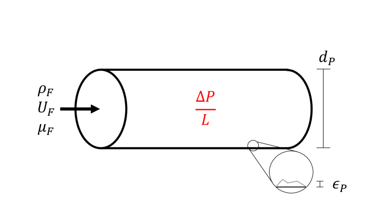
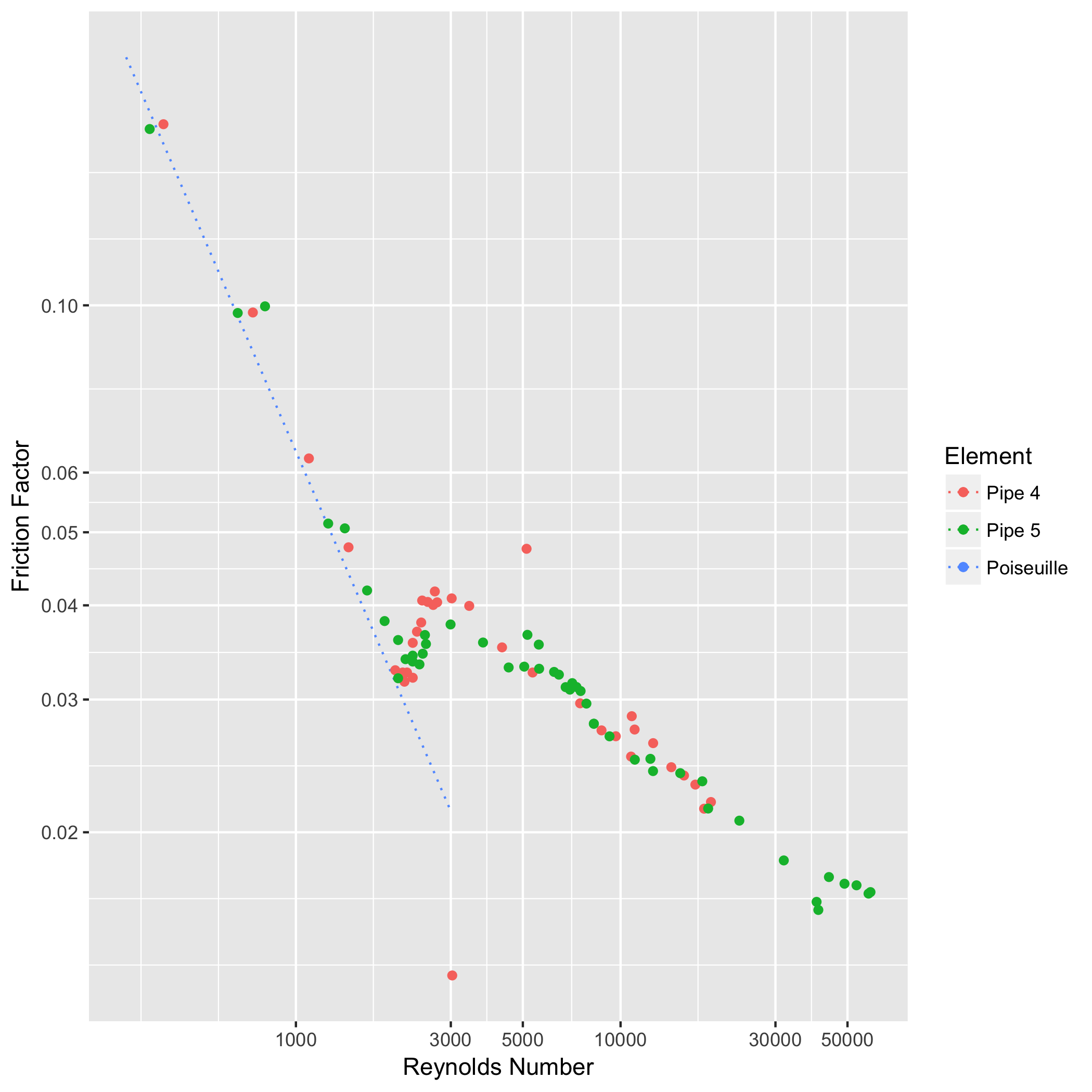
In his seminal paper, Osborne Reynolds [22] considered the effects of the fluid bulk velocity $U_{F}$, density $\rho_{F}$, and viscosity $\mu_{F}$, as well as the pipe diameter $d_{P}$ on qualitative and quantitative behavior of the resulting flow. To apply Dimensional Analysis, one must first write down the physical dimensions of the variables, as shown in Table 2. This dimension matrix has a one-dimensional nullspace, for which the vector $(1,1,1,-1)^{T}$ is a basis. The corresponding dimensionless quantity is $\rho_{F}U_{F}d_{F}/\mu_{F}$, which was first considered by Reynolds in his 1883 work.

Dimension	$\rho_{F}$	$U_{F}$	$d_{P}$	$\mu_{F}$
Mass (M)	1	0	0	1
Length (L)	0 $-$ 3	1	1	0 $-$ 1
Time (T)	0	0 $-$ 1	0	0 $-$ 1

Table 2: Dimension matrix for Rough Pipe Flow, neglecting roughness.

Reynolds found that his own data collapsed to a one dimensional function against this dimensionless quantity (Fig. 1), and so applied his findings to the data of Henry Darcy. Darcy had considered a number of pipes of different materials, and Reynolds found he needed to apply a correction term in order to bring the different datasets into agreement. Reynolds noted

“Darcy’s pipes were all of them uneven between the gauge points, the glass and the iron varying as much as 20 per cent.(sic) in section. The lead were by far the most uniform, so that it is not impossible that the differences in the values of $n$ may be due to this unevenness. But the number of joins and unevenness of the tarred pipes corresponded very nearly with the new cast iron, and between these there is a very decided difference in the value of $n$. This must be attributed to the roughness of the cast iron surface.”

Reynolds correctly deduced the significance of the pipe roughness using prior experience, but did not include a variable to represent it in his 1883 work. One may regard roughness $\epsilon_{P}$ as a lurking variable in Reynolds’ original setting. Reynolds manufactured two pipes (Pipe No. 4 and Pipe No. 5) of varying diameter but the same material, varying $d_{P}$ but leaving $\epsilon_{P}$ fixed. This feature of the experiment would have rendered lurking variable detection via the usual approaches impossible. Could an experimentalist have detected the lurking roughness through a statistical approach? We will provide evidence of an affirmative answer through the examples below, but first provide some intuition for how such a procedure is possible.

Note that considering all the salient factors for Rough Pipe Flow yields the dimension matrix shown in Table 1. This matrix has a two-dimensional nullspace, for which an acceptable basis is $\{(1,1,1,-1,0)^{T},(0,-1,0,0,1)^{T}\}$. These vectors correspond respectively to the Reynolds number and the relative roughness $\epsilon_{P}/d_{P}$.[18] Note that in Reynolds’ setting, the observed variables are $\{\rho_{F},U_{F},d_{P},\mu_{F}\}$ while the sole lurking variable is $\epsilon_{P}$. In this case there is only one predicted dimensionless quantity, and so naive Dimensional Analysis suggests the response is one-dimensional in $Re$. However, the true physical relationship depends additionally on the relative roughness $\epsilon_{P}/d_{P}$; this results in additional variability due to $d_{P}$, and in two-dimensional behavior unpredicted by Dimensional Analysis on the observed variables alone. One could attempt to perform visual inspection based on the predicted dimensionless quantities; however, we will instead build a formal hypothesis test. Below, we present a modified version of Buckingham $\pi$, first shown by Constantine et al.[10] This provides a sufficient dimension reduction based on a priori knowledge, contingent on the absence of lurking variables.[2] This is the key to our lurking variable detection strategy.

2.3 The Pi Subspace and lurking variables

The effect of the $\log$ operator is to turn power-products into linear combinations. If we define $\boldsymbol{x}\equiv\log(\boldsymbol{z})\in\mathbb{R}^{p}$, with the $\log$ (and $\exp$ to follow) interpreted in the elementwise sense, we may rewrite the Buckingham $\pi$ theorem as

$$\pi =f(\boldsymbol{z}),$$ (3)

$$=\psi(\pi_{1},\dots,\pi_{p-r}),$$

$$=\psi^{\prime}(\boldsymbol{V}^{T}\boldsymbol{x}),$$

where $\psi^{\prime}(\boldsymbol{\xi})=\psi(\exp(\boldsymbol{\xi}))$, and $\boldsymbol{V}\in\mathbb{R}^{p\times(p-r)}$ is a basis for the nullspace of $\boldsymbol{D}$. Let $\mathcal{R}(\boldsymbol{A})$ denote the columnspace of a matrix $\boldsymbol{A}$. The subspace $\mathcal{R}(\boldsymbol{V})$ is known from $\boldsymbol{D}$; if all the physical inputs $\boldsymbol{z}$ have been correctly identified, then $\boldsymbol{D}$ is known a priori. Suppose that $\pi$ is measured via some noisy instrument. Then $\pi=\psi^{\prime}(\boldsymbol{V}^{T}\boldsymbol{x})+\epsilon^{\prime}$. If we assume $\epsilon^{\prime}$ to be unbiased, we have

$$\pi|\boldsymbol{x}\sim\pi|\boldsymbol{V}^{T}\boldsymbol{x};$$ (4)

that is, $\mathcal{R}(\boldsymbol{V})$ is a sufficient dimension reduction.[2] Intuitively, a subspace is sufficient if it captures all available information about a qoi; moving orthogonal to $\boldsymbol{V}$ results in no change to $\pi$ outside random fluctuations. Since $\mathcal{R}(\boldsymbol{V})$ is determined from the Buckingham $\pi$ theorem, we call it the pi subspace. Note that while the pi subspace is uniquely determined by $\boldsymbol{D}$, the matrix $\boldsymbol{V}$ must be chosen. Selecting an appropriate $\boldsymbol{V}$ is certainly of interest; both in engineering [12] and statistical circles [23]. However, in what follows we need only $\mathcal{R}(\boldsymbol{V})$, so the precise choice of $\boldsymbol{V}$ is not an issue we consider in this work.

Of greater import in this discussion is the choice of $\boldsymbol{x}$ (equivalently $\boldsymbol{z}$). An analyst chooses the relevant physical quantities based on previous experience or intuition. Previous experience may fail to generalize, and intuition can be faulty. In these cases, even an experienced investigator may fail to identify all the relevant factors, and may instead consider $p_{E}<p$ observed or exposed variables $\boldsymbol{x}_{E}\in\mathbb{R}^{p_{E}}$, leaving out $p-p_{E}$ lurking variables $\boldsymbol{x}_{L}\in\mathbb{R}^{p-p_{E}}$. Note that the ordering of variables in $\boldsymbol{x}$ is arbitrary; we assume an ordering and write

$$\boldsymbol{x}^{T}=(\boldsymbol{x}_{E}^{T},\boldsymbol{x}_{L}^{T}).$$ (5)

The analyst varies $\boldsymbol{x}_{E}$ in order to learn about the functional dependence of the qoi on these exposed variables. In practice, the analyst is aware of $\boldsymbol{x}_{E}$ and their physical dimensions $\boldsymbol{D}_{E}\in\mathbb{R}^{d\times p_{E}}$, but is totally ignorant of $\boldsymbol{x}_{L}$ and their physical dimensions $\boldsymbol{D}_{L}\in\mathbb{R}^{d\times(p-p_{E})}$. The full dimension matrix is then $\boldsymbol{D}=[\boldsymbol{D}_{E},\boldsymbol{D}_{L}]$. In such a setting, the analyst would derive an incorrect pi subspace corresponding to $\boldsymbol{V}^{\prime}_{E}\in\mathbb{R}^{p_{E}\times(p_{E}-r_{E})}$, where $\boldsymbol{D}_{E}\boldsymbol{V}^{\prime}_{E}=0$. This is a recognized issue in the study of Dimensional Analysis.[24] In the case where $\mathcal{R}(\boldsymbol{V}^{\prime}_{E})\not\supseteq\mathcal{R}(\boldsymbol{V})$, the derived subspace will not be sufficient. Note that the Buckingham $\pi$ theorem constrains the gradient of our qoi to live within the pi subspace; we may use this fact to provide diagnostic information.

Note that

$$\nabla_{\boldsymbol{x}}^{T}\pi=(\nabla_{\boldsymbol{x}_{E}}^{T}\pi,\nabla_{\boldsymbol{x}_{L}}^{T}\pi).$$ (6)

Since $\boldsymbol{D}\nabla_{\boldsymbol{x}}\pi=0$, we have

$$\boldsymbol{D}_{E}\nabla_{\boldsymbol{x}_{E}}\pi=-\boldsymbol{D}_{L}\nabla_{\boldsymbol{x}_{L}}\pi.$$ (7)

Equation 7 demonstrates that the vector of physical dimensions of the exposed variables matches that of the lurking variables. Furthermore, the left-hand side of (7) is composed of known (or estimable) quantities. If $\boldsymbol{D}_{E}\nabla_{\boldsymbol{x}_{E}}\pi$ is nonzero, it signals that 1) a lurking variable exists, and 2) it possesses physical dimensions aligned with $\boldsymbol{D}_{L}\nabla_{\boldsymbol{x}_{L}}\pi$. In the Rough Pipe Flow example, the entries of $\boldsymbol{D}_{E}\nabla_{\boldsymbol{x}_{E}}\pi$ correspond to Mass, Length, and Time, respectively. Thus if $\boldsymbol{D}_{E}\nabla_{\boldsymbol{x}_{E}}\pi=(0,c,0^{T})$, a lurking lengthscale affects the qoi. The information provided is richer than a simple binary detection; we can gleam some physical information about the lurking variable. To capitalize on this observation, we will base our detection procedure on estimating the gradient of our quantity of interest.

There are important caveats to note. We may have $\boldsymbol{D}_{L}=0$ (i.e. the $\boldsymbol{z}_{L}$ are dimensionless), or we may have dimensional inputs but $\nabla_{\boldsymbol{x}_{L}}\pi\neq 0$ with $\boldsymbol{D}_{L}\nabla_{\boldsymbol{x}_{L}}\pi=0$ (i.e. the lurking variables form a dimensionless quantity). The latter case is unlikely; this occurs when the analyst truly does not know much about the problem at hand. The former case is more challenging – natural physical quantities exist that are inherently dimensionless, such as angles. To combat these issues, an analyst may choose to decompose such dimensionless quantities in terms of other dimensional ones; an angle may be considered a measure between two vectors, so an analyst may introduce lengthscales that form the desired angle. However, this requires intimate understanding of the failure mode, and does not address the fundamental issue. In the case where such an unknown is dimensionless, detection must be based on some other principle, as Dimensional Analysis will not be of help.

2.4 Non-dimensionalization

Rarely is a measured qoi dimensionless; usually, a dimensionless qoi must be derived via non-dimensionalization. Given some dimensional qoi $q$, we form the non-dimensionalizing factor via a product of the physical input factors $\exp(\boldsymbol{u}^{T}\boldsymbol{x})=\prod_{i=1}^{p}z_{i}^{u_{i}}$, such that $\boldsymbol{d}(q)=\boldsymbol{d}(\prod_{i=1}^{p}z_{i}^{u_{i}})$. We then form the dimensionless qoi via

$$\pi(\boldsymbol{x}) =q(\boldsymbol{x})\prod_{i=1}^{p}z_{i}^{-u_{i}},$$ (8)

$$=q(\boldsymbol{x})\exp(-\boldsymbol{u}^{T}\boldsymbol{x}).$$

One may determine an acceptable non-dimensionalizing factor by solving the linear system

$$\boldsymbol{d}(q)=\boldsymbol{D}\boldsymbol{u}.$$ (9)

If (9) possesses no solution, then no dimensionally homogeneous relationship among the qoi and proposed variables exists. Since the physical world is required to be dimensionally homogeneous, we conclude that lurking variables must affect the qoi. Bridgman [7, Ch. 1] illustrates this point through various examples.

More commonly, Equation 9 will possess infinite solutions; however, under sensible conditions (Sec. 8.1), there exists a unique $\boldsymbol{u}^{*}$ that is orthogonal to the pi subspace, i.e. $\boldsymbol{V}^{T}\boldsymbol{u}^{*}=0$. This is useful in the case where we cannot measure $\pi$ directly, but must instead observe $q_{\text{obs}}$; the physical qoi subject to some added noise $\epsilon$. In Box’s [6] formulation, this $\epsilon$ represents additional, randomly fluctuating lurking variables. In this case

$$q_{\text{obs}}(\boldsymbol{x}) =q(\boldsymbol{x})+\epsilon,$$ (10)

$$\pi_{\text{obs}}(\boldsymbol{x}) =\pi(\boldsymbol{x})+\epsilon\exp(-\boldsymbol{u}^{T}\boldsymbol{x}).$$

In principle, the orthogonality condition $\boldsymbol{V}^{T}\boldsymbol{u}=0$ could aid in separating signal from noise. However, we shall see that so long as the noise term is unbiased, we may use the heteroskedastic form of (10).

2.5 Pinned variables

Above, we have implicitly assumed that the $\boldsymbol{x}_{E}$ are varied experimentally. In some cases, a variable is known but intentionally not varied by the experimentalist. We call these known but fixed quantities pinned variables. The decision to pin a variable may be due to cost or safety constraints. With some modifications, Dimensional Analysis may still be employed for lurking variable detection in this setting. For a pinned variable, we have knowledge of its physical dimensions $\boldsymbol{D}_{P}$. We may split $\boldsymbol{x}$ in a form similar to (5)

$$\boldsymbol{x}^{T}=(\boldsymbol{x}_{E}^{T},\boldsymbol{x}_{L}^{T},\boldsymbol{x}_{P}^{T}),$$ (11)

note that $\boldsymbol{D}=[\boldsymbol{D}_{E},\boldsymbol{D}_{L},\boldsymbol{D}_{P}]$, and write a relation analogous to (7)

$$\boldsymbol{D}_{E}\nabla_{\boldsymbol{x}_{E}}\pi=-\boldsymbol{D}_{P}\nabla_{\boldsymbol{x}_{P}}\pi-\boldsymbol{D}_{L}\nabla_{\boldsymbol{x}_{L}}\pi.$$ (12)

If no lurking variables exist, then the quantity $\boldsymbol{D}_{E}\nabla_{\boldsymbol{x}_{E}}\pi$ is expected to lie in the range of $\boldsymbol{D}_{P}$. One can use this information to construct a detection procedure, so long as $\mathcal{R}(\boldsymbol{D}_{L})\not\subseteq\mathcal{R}(\boldsymbol{D}_{P})$. In the case where $\mathcal{R}(\boldsymbol{D}_{P})=\mathbb{R}^{d}$, detecting lurking variables via dimensional analysis using (12) is impossible, as $\mathcal{R}(\boldsymbol{D}_{L})\subseteq\mathcal{R}(\boldsymbol{D}_{P})$.

Suppose $\mathcal{R}(\boldsymbol{D}_{P})\subset\mathbb{R}^{d}$ with $\text{Rank}(\boldsymbol{D}_{P})=r_{P}<d$, and let $\boldsymbol{W}_{P}\in\mathbb{R}^{d\times(d-r_{P})}$ be an orthonormal basis for the orthogonal complement of $\boldsymbol{D}_{P}$; that is $\boldsymbol{W}_{P}^{T}\boldsymbol{W}_{P}=\boldsymbol{I}_{(d-r_{P})\times(d-r_{P})}$ and $\boldsymbol{W}^{T}_{P}\boldsymbol{D}_{P}=0$. Then we have

$$\boldsymbol{W}_{P}^{T}\boldsymbol{D}_{E}\nabla_{\boldsymbol{x}_{E}}\pi=-\boldsymbol{W}_{P}^{T}\boldsymbol{D}_{L}\nabla_{\boldsymbol{x}_{L}}\pi.$$ (13)

So long as $\boldsymbol{W}_{P}^{T}\boldsymbol{D}_{L}\neq 0$, Equation 13 may enable lurking variable detection. Note that if $\mathcal{R}(\boldsymbol{D}_{P})\notperp\mathcal{R}(\boldsymbol{D}_{L})$, then multiplying by $\boldsymbol{W}_{P}^{T}$ will eliminate some information in $\boldsymbol{D}_{L}\nabla_{\boldsymbol{x}_{L}}\pi$. Thus, while detection is possible with (13), interpreting the dimension vector requires more care.

3 Constructing a Detection Procedure

This section details the requisite machinery for our experimental lurking variable detection procedures, which ultimately consist of an experimental design coupled with a hypothesis test. Stein’s lemma guides the design and enables the definition of our null and alternative hypotheses, while Hotelling’s $T^{2}$ test provides a suitable statistic.

3.1 Stein’s Lemma

Computing the gradient is challenging in the context of a physical experiment. The usual approximation techniques of finite differences can be inappropriate in this setting, where experimental noise may dwarf perturbations to the factors, and arbitrary setting of levels may be impossible. We do not address the latter issue and assume continuous variables, but attack the former by pursuing a different tack, that of approximating the average gradient through experimental design.

Stein’s lemma was originally derived in the context of mean estimation; in our case, we will use it to derive an estimate of the average gradient from point evaluations of the qoi.[25, 16] If $X\sim N(\boldsymbol{\mu},\boldsymbol{\Sigma})$ where $N(\boldsymbol{\mu},\boldsymbol{\Sigma})$ is a multivariate normal distribution with mean $\boldsymbol{\mu}$ and invertible covariance matrix $\boldsymbol{\Sigma}$, Stein’s lemma states

$$\mathbb{E}[\nabla_{\boldsymbol{x}}f(X)]=\boldsymbol{\Sigma}^{-1}\mathbb{E}[(X-\boldsymbol{\mu})f(X)].$$ (14)

We will assume in what follows that the exposed parameters are independent and free to be drawn according to $\boldsymbol{x}_{E}\sim N(\boldsymbol{\mu}_{E},\boldsymbol{\Sigma}_{E})$, with $\boldsymbol{\mu}_{E}$ and $\boldsymbol{\Sigma}_{E}$ invertible selected by the experimentalist, in order to study a desired range of values. Furthermore, we assume our quantity of interest $q$ is dimensional, and subject to $\boldsymbol{x}_{E}$ -independent, zero-mean noise $\epsilon$. Taking an expectation with respect to both $\boldsymbol{x}_{E}$ and $\epsilon$, and applying Stein’s lemma to the second line of (10) yields

$$\mathbb{E}[\boldsymbol{\Sigma}_{E}^{-1}(\boldsymbol{x}_{E}-\boldsymbol{\mu}_{E})\pi_{\text{obs}}(\boldsymbol{x}_{E},\boldsymbol{x}_{L})] =\mathbb{E}[\nabla_{\boldsymbol{x}_{E}}\pi(\boldsymbol{x}_{E},\boldsymbol{x}_{L})]$$ (15)

$$+\mathbb{E}[\nabla_{\boldsymbol{x}_{E}}\exp(-\boldsymbol{w}_{E}^{T}\boldsymbol{x}_{E})\epsilon].$$

Note that the noise term vanishes due to its zero-mean. Multiplying by the dimension matrix yields

$$\mathbb{E}[\boldsymbol{D}_{E}\boldsymbol{\Sigma}_{E}^{-1}(\boldsymbol{x}_{E}-\boldsymbol{\mu}_{E})\pi_{\text{obs}}(\boldsymbol{x}_{E},\boldsymbol{x}_{L})]=\mathbb{E}[\boldsymbol{D}_{E}\nabla_{\boldsymbol{x}_{E}}\pi(\boldsymbol{x}_{E},\boldsymbol{x}_{L})].$$ (16)

Equation 16 enables the definition of an appropriate null hypothesis $H_{0}$ for lurking variable testing. We denote by $H_{0}$ the null hypothesis of no dimensional lurking variables, and by $H_{1}$ the alternative of present lurking variables. These hypotheses are defined by

$$H_{0}:\mathbb{E}[\boldsymbol{D}_{E}\boldsymbol{\Sigma}_{E}^{-1}(\boldsymbol{x}_{E}-\boldsymbol{\mu}_{E})\pi_{\text{obs}}(\boldsymbol{x}_{E},\boldsymbol{x}_{L})]=0,$$ (17)

$$H_{1}:\mathbb{E}[\boldsymbol{D}_{E}\boldsymbol{\Sigma}_{E}^{-1}(\boldsymbol{x}_{E}-\boldsymbol{\mu}_{E})\pi_{\text{obs}}(\boldsymbol{x}_{E},\boldsymbol{x}_{L})]=\boldsymbol{\nu}.$$

Our procedure for dimensional lurking variables is built upon a test for zero mean of a multivariate distribution. To define a test statistic, we turn to Hotelling’s $T^{2}$ test.

3.2 Hotelling’s T-squared test

Hotelling’s $T^{2}$ test is a classical multivariate generalization of the t-test.[4] We draw $n>d$ samples according to the design $\boldsymbol{x}_{E,i}\sim N(\boldsymbol{\mu}_{E},\boldsymbol{\Sigma}_{E})$ with $i=1,\dots,n$, and based on evaluations

$$\boldsymbol{g}_{i}=\boldsymbol{D}_{E}\boldsymbol{\Sigma}_{E}^{-1}(\boldsymbol{x}_{E,i}-\boldsymbol{\mu}_{E})\pi_{\text{obs}}(\boldsymbol{x}_{E,i},\boldsymbol{x}_{L})\in\mathbb{R}^{d},$$ (18)

define our $t$ statistic via

$$t^{2}=n\bar{\boldsymbol{g}}^{T}\hat{\boldsymbol{S}}^{-1}\bar{\boldsymbol{g}},$$ (19)

where $\bar{\boldsymbol{g}}$ is the sample mean of the $\boldsymbol{g}_{i}$, and $\hat{\boldsymbol{S}}$ is the sample covariance

$$\hat{\boldsymbol{S}}=\frac{1}{n-1}\sum_{i=1}^{n}(\boldsymbol{g}_{i}-\bar{\boldsymbol{g}})(\boldsymbol{g}_{i}-\bar{\boldsymbol{g}})^{T}.$$ (20)

Under a normal $\boldsymbol{g}_{i}$ assumption and $H_{0}$, Equation 19 follows the distribution

$$t^{2}\sim T^{2}_{d,n-1}=\frac{d(n-1)}{n-d}F_{d,n-d},$$ (21)

where $F_{d,n-d}$ is the central F-distribution with parameters $d$ and $n-d$. Note that even with $\boldsymbol{x}_{E}$ and $\epsilon$ normal, the $\boldsymbol{g}_{i}$ are not necessarily normal, as $q(\boldsymbol{x})$ may be an arbitrary function. While the derivation of the reference distribution (21) requires normality, it is well-known that the associated test is robust to departures from this assumption.[15, 17] Given this robustness, (21) allows effective testing of $H_{0}$. This claim will be further substantiated in Section 5 below.

Suppose we are testing at the $\alpha$ level; let $F_{d,n-d}^{c}(\alpha)$ be the critical test value based on the inverse CDF for $F_{d,n-d}$. We reject $H_{0}$ if

$$t^{2}\geq\frac{d(n-1)}{n-d}F_{d,n-d}^{c}(\alpha).$$ (22)

3.3 Factors affecting power

From (7) and (16), we know $\boldsymbol{\nu}=-\mathbb{E}[\boldsymbol{D}_{L}\nabla_{\boldsymbol{x}_{L}}\pi]$. Note that the first two moments of $\boldsymbol{g}$ are

$$\mathbb{E}[\boldsymbol{g}] \equiv\boldsymbol{\nu}=\mathbb{E}[\boldsymbol{D}_{E}\nabla_{\boldsymbol{x}_{E}}\pi],$$ (23)

$$\mathrm{V}[\boldsymbol{g}] =\mathbb{E}[\boldsymbol{g}\boldsymbol{g}^{T}]-\boldsymbol{\nu}\boldsymbol{\nu}^{T}.$$

In the case where $H_{1}$ holds, under a normal $\boldsymbol{g}$ we find that the test statistic (19) instead follows[4]

$$t^{2}\sim\frac{d(n-1)}{n-d}F_{d,n-d}(\Delta),$$ (24)

where $F_{d,n-d}(\Delta)$ is a non-central F-distribution with non-centrality parameter

$$\Delta=n\mathbb{E}[\boldsymbol{g}]^{T}\mathrm{V}[\boldsymbol{g}]^{-1}\mathbb{E}[\boldsymbol{g}],$$ (25)

which implies $\Delta\geq 0$. The power $P$ of our test is then given by

$$P\equiv\mathbb{P}\left[F_{d,n-d}(\Delta)\geq F_{d,n-d}^{c}(\alpha)\left|H_{1}\right.\right].$$ (26)

Equation 26 implies that larger values of $\Delta$ lead to higher power. To better understand the contributions to (25), we apply the Sherman-Morrison formula to $\mathrm{V}[\boldsymbol{g}]$ to separate contributions of $\boldsymbol{\nu}$ and other variance components. Doing so yields

$$\Delta=n\left(k+\frac{k^{2}}{1-k}\right),$$ (27)

where $k=\boldsymbol{\nu}^{T}\mathbb{E}[\boldsymbol{g}\boldsymbol{g}^{T}]^{-1}\boldsymbol{\nu}$. It is easy to see that $k\in[0,1]$. Based on (27), we see that power is an increasing function of $n$ and $k$. However, Taylor expanding $\pi(\boldsymbol{x})$ about $\boldsymbol{\mu}$ reveals that $\boldsymbol{\nu}$ and $\mathbb{E}[\boldsymbol{g}\boldsymbol{g}^{T}]$ have different dependencies on the moments of the sampling distribution, and therefore different dependencies on $\boldsymbol{\mu}_{E},\boldsymbol{\Sigma}_{E}$. Thus, the dependence of power (via $k$) on the sampling distribution cannot be known without more knowledge of the functional form of $\pi(\boldsymbol{x})$. For instance, it is easy to construct simple examples of $\pi(\boldsymbol{x})$ which limit to either power of zero or power of one while scaling $\boldsymbol{\Sigma}_{E}$ towards zero or infinity.

To see the impact of noise on power, we consider the average outer-product of the test statistic, given by

$$\mathbb{E}[\boldsymbol{g}\boldsymbol{g}^{T}]=\boldsymbol{D}_{E}\boldsymbol{\Sigma}_{E}^{-1}\mathbb{E}[(\boldsymbol{x}_{E}-\boldsymbol{\mu}_{E})(\boldsymbol{x}_{E}-\boldsymbol{\mu}_{E})^{T}(\pi^{2}+\exp(-2\boldsymbol{w}_{E}^{T}\boldsymbol{x}_{E})\tau^{2})]\boldsymbol{\Sigma}_{E}^{-1}\boldsymbol{D}_{E}^{T},$$ (28)

where $\tau^{2}$ is the variance of $\epsilon$. Through multiple applications of Jensen’s inequality, we may show

$$\boldsymbol{D}_{E}\boldsymbol{\Sigma}_{E}^{-1}\mathbb{E}[(\boldsymbol{x}_{E}-\boldsymbol{\mu}_{E})(\boldsymbol{x}_{E}-\boldsymbol{\mu}_{E})^{T}\exp(-2\boldsymbol{w}^{T}_{E}\boldsymbol{x}_{E})\tau^{2}]\boldsymbol{\Sigma}_{E}^{-1}\boldsymbol{D}_{E}^{T}\geq(\boldsymbol{D}_{E}\boldsymbol{w}_{E})(\boldsymbol{D}_{E}\boldsymbol{w}_{E})^{T}\tau^{2}/\bar{Q}^{2}\geq 0,$$ (29)

where $\bar{Q}\equiv\exp(-\boldsymbol{w}_{E}^{T}\boldsymbol{\mu})$. Since $\mathbb{E}[\boldsymbol{g}\boldsymbol{g}^{T}]$ enters as an inverse, Equation 29 shows that the noise variability $\tau$ negatively affects power, as is intuitively expected. However, since this term is added with the qoi-dependent term, one cannot know an appropriate scale for $\tau$ without more knowledge of the structure of $\pi(\boldsymbol{x})$. We will see below that the effects of noise can be similar across disparate values of $\tau/\bar{Q}$.

4 Detecting Lurking Variables

In this section, we present procedures for lurking variable detection. The first procedure is based entirely upon a priori information. The second combines Dimensional Analysis (Sec. 2) with the statistical machinery introduced above (Sec. 3). The final procedure is a modification of the second, introduced to handle pinned variables. Examples of these procedures are presented below, in Section 5.

4.1 Detection with a priori information

In some cases, the analyst may detect lurking variables based solely on a priori information. This can be done with a simple analytic check for dimensional homogeneity. In the case where no non-dimensionalizing factor can be defined; that is $\boldsymbol{d}(q)\not\in\mathcal{R}(\boldsymbol{D}_{E})$, dimensional homogeneity cannot hold. This is a clear signal that lurking variables affect our qoi.

4.2 Detection with a physical qoi

This subsection lays out a three-step procedure to test for lurking variables. Note that in what follows, the lurking variables need not vary, and are assumed to be fixed throughout the experiment.

This procedure assumes the following setting: Let $q$ be a physical quantity of interest, with identified predictors $\boldsymbol{x}_{E}\in\mathbb{R}^{p_{E}}$ and physical dimensions $\boldsymbol{D}_{E}\in\mathbb{R}^{d\times p_{E}}$. Assume $\boldsymbol{d}(q)\in\mathcal{R}(\boldsymbol{D}_{E})$, and that one may vary the $\boldsymbol{x}_{E}$ within acceptable bounds and evaluate $q_{\text{obs}}(\boldsymbol{x}_{E})$ via the experimental setup.

Step 1: Perform dimensional analysis

Solve $\boldsymbol{d}(q)=\boldsymbol{D}_{E}\boldsymbol{w}_{E}$ for $\boldsymbol{w}_{E}\in\mathbb{R}^{p_{E}}$; this enables computation of

$$\pi_{\text{obs}}(\boldsymbol{x}_{E})=q_{\text{obs}}(\boldsymbol{x}_{E})\exp(-\boldsymbol{w}_{E}^{T}\boldsymbol{x}_{E}).$$

Step 2: Design and perform experiment

Choose $\boldsymbol{\mu}_{E}\in\mathbb{R}^{d_{E}}$ and $\boldsymbol{\Sigma}_{E}\in\mathbb{R}^{p_{E}\times p_{E}}$ in order to select a range of values for study. Draw samples $\boldsymbol{x}_{E}\sim N(\boldsymbol{\mu}_{E},\boldsymbol{\Sigma}_{E})$ with $i=1,\dots,n$. Evaluate $q_{\text{obs}}(\boldsymbol{x}_{E})$ via the experimental setup, and use $\boldsymbol{w}_{E}$ from Step 1 to compute $\pi_{\text{obs}}(\boldsymbol{x}_{E})$.

Step 3: Test

Select a confidence level, form the $\boldsymbol{g}_{i}$ defined by (18), compute $t^{2}$ via (19), and compare against the reference distribution defined by (21). If $t^{2}$ is larger than the critical value, reject the null hypothesis of no lurking variables.

4.3 Detection in the presence of pinned variables

If a pinned variable affects our qoi, the detection procedure defined above is inappropriate. In this case, we recommend a simple modification to the procedure above, based on (13). In what follows, we assume the same setting as Section 4.2, with the addition of $\boldsymbol{x}_{P}\in\mathbb{R}^{p_{P}}$ pinned variables, with known dimensions $\boldsymbol{D}_{P}\in\mathbb{R}^{d\times p_{P}}$. These $\boldsymbol{x}_{P}$ remain fixed throughout the experiment. As mentioned in Section 2.5, interpretation of the dimension vector requires more care.

Step 1: Perform dimensional analysis

Determine $r_{P}=\text{Rank}(\boldsymbol{D}_{P})$, and check that $r_{P}<d$. If so, compute a basis $\boldsymbol{W}_{P}\in\mathbb{R}^{d\times(d-r_{P})}$ for the orthogonal complement of $\boldsymbol{D}_{P}$, e.g. via a QR decomposition.

Step 2: Design and perform experiment

This step remains unchanged; note that $\boldsymbol{x}_{E}$ refers only to those variables which can be varied.

Step 3: Test

Follow Step 3 above, but modify the $\boldsymbol{g}_{i}$ as defined by (18)

$$\boldsymbol{g}^{\prime}_{i}=\boldsymbol{W}_{P}^{T}\boldsymbol{g}_{i}.$$ (30)

Compute $t^{2}$ via (19) based on the $\boldsymbol{g}^{\prime}_{i}$; note that $d$ is replaced with $d-r_{P}$ for this modified statistic. If $t^{2}\geq\frac{(d-r_{P})(n-1)}{n-d+r_{P}}F_{p_{P},n-d+r_{P}}^{c}(\alpha)$, then reject $H_{0}$.

5 Detection Examples

5.1 Physical examples

In what follows, we consider two physical examples motivated by engineering applications: Rough Pipe Flow and Two-Fluid Flow. This section gives a short description of the examples; full details, including derivations and code sufficient to reproduce all results below, are available in the Supporting Material. Rough Pipe Flow has already been introduced above in Section 2.2; the full list of the predictors, the response, and associated physical dimensions is detailed in Table 3. For Rough Pipe Flow, evaluation of the qoi is based on analytic and empirical relationships: Poiseuille’s law for laminar flow, and the Colebrook equation to model behavior from the turbulent onset to full turbulence.[30, 9]

Physical Variable	Symbol	Physical Dimensions
Pressure Gradient (qoi)	$\frac{\Delta P}{L}$	$M^{1}L^{-1}T^{-2}$
Pipe Diameter	$d_{P}$	$L$
Pipe Roughness	$\epsilon_{P}$	$L$
Fluid Bulk Velocity	$U_{F}$	$L^{1}T^{-1}$
Fluid Density	$\rho_{F}$	$M^{1}L^{-3}$
Fluid Viscosity	$\mu_{F}$	$M^{1}L^{-1}T^{-1}$

Table 3: Physical variables for Rough Pipe Flow.

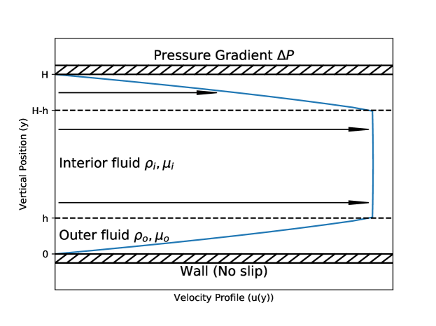
The second example is Two-Fluid Flow, inspired by an engineering need to pump viscous fluids at a high rate. In this setting, two immiscible fluids are assumed to be in steady laminar flow through a channel. The fluids form layers depicted in Figure 2, where the inner fluid is assumed to be more viscous than the outer fluid ($\mu_{i}>>\mu_{o}$). This outer lubricating layer allows faster transport of the inner fluid, but reduces the effective diameter for pumping. The qoi is the volumetric flow rate of the inner flow. In this example, evaluation of the qoi is based on an analytic expression, derived from the Navier-Stokes equations with some standard simplifying assumptions.[30]

Figure 2: Schematic for Two-Fluid Flow. The view is of a cross-section of an infinite channel formed by two parallel plates. A viscous fluid flows in the cavity between these two surfaces. Fluid flows from left to right, and the velocity profile (depicted in blue) across the channel is shown; zero velocity corresponds to the left boundary of the figure, while positions on the curve further to the right correspond to greater velocity. The dashed horizontal lines illustrate the boundary between the inner and outer fluids; the qoi is the flow rate between the two dashed lines. By design, the flow rate is nearly independent of the inner flow fluid properties.

In this example, the qoi is significantly less sensitive to the inner fluid properties than the other factors. This is by design. Since our lurking variable detection procedure is based on the sensitivity of the qoi to the lurking variable in question, detecting a lurking inner fluid property is challenging. Note also that formally, the dimensional qoi is not sensitive to the fluid densities. These predictors are included to demonstrate that our procedure handles such unimportant variables automatically.

Physical Variable	Symbol	Physical Dimensions
Flow Rate (qoi)	$q$	$L^{2}T^{-1}$
Applied Pressure Gradient	$\nabla P$	$M^{1}L^{-2}T^{-2}$
Outer Fluid Thickness	$h$	$L$
Inner Fluid Thickness	$H$	$L$
Outer Fluid Viscosity	$\mu_{o}$	$M^{1}L^{-1}T^{-1}$
Inner Fluid Viscosity	$\mu_{i}$	$M^{1}L^{-1}T^{-1}$
Outer Fluid Density	$\rho_{o}$	$M^{1}L^{-3}$
Inner Fluid Density	$\rho_{i}$	$M^{1}L^{-3}$

Table 4: Physical variables for Two-Fluid Flow

5.2 Analytic detection

As a concrete example of the analytic detection procedure, consider the problem of Rough Pipe Flow. Suppose an analyst believes that the pipe diameter $d_{P}$ and fluid bulk velocity $U_{F}$ are the only factors which affect the qoi. In this case, the reduced dimension matrix is given in Table 5.

Dimension	$d_{P}$	$U_{F}$	$\Delta P$
Mass (M)	0	0	1
Length (L)	1	1	0 $-$ 1
Time (T)	0	0 $-$ 1	0 $-$ 2

Table 5: Reduced dimension matrix for Rough Pipe Flow. The center columns are $\boldsymbol{D}_{E}$, while the rightmost column is $\boldsymbol{d}(q)$. In this case, it is evident that dimensional homogeneity cannot hold, and a lurking variable must exist.

By inspection, we can see $\boldsymbol{d}(q)\not\in\mathcal{R}(\boldsymbol{D}_{E})$. One cannot form a non-dimensionalizing factor from the given predictors; clearly something is missing. Note that none of the proposed predictors has physical dimensions of Mass; this hints that the lurking variables must introduce a Mass.

The analysis above can be performed without experimentation, but it is extremely limited. Suppose that an analyst instead proposed predictors of fluid density $\rho_{F}$ and bulk velocity $U_{F}$. Then the reduced dimension matrix is given in Table 6. In this case, dimensional homogeneity holds, and the analyst can form a non-dimensionalizing factor; the dynamic pressure $\frac{1}{2}\rho_{F}U_{F}^{2}$.[30] To learn more, the analyst must turn to fluid mechanics; either analytic or experimental.

Dimension	$\rho_{F}$	$U_{F}$	$\Delta P$
Mass (M)	1	0	1
Length (L)	0 $-$ 3	1	-1
Time (T)	0	0 $-$ 1	-2

Table 6: Reduced dimension matrix for Rough Pipe Flow. The center columns are $\boldsymbol{D}_{E}$, while the rightmost column is $\boldsymbol{d}(q)$. In this case, one can form the dynamic pressure $\frac{1}{2}\rho_{F}U_{F}^{2}$, which is a suitable non-dimensionalizing factor for the qoi. To learn more, an experimentalist could collect data to probe the the functional relationship between the response and predictors. This would reveal additional variability not predicted by naive Dimensional Analysis.

5.3 Experimental detection

In this section, we perform numerical experiments to test the assumptions introduced in Section 4 above, and assess the efficacy of the proposed detection procedures. In the following examples, we query an R implementation of the models above to perform virtual experiments.[21, 31, 29, 13, 11] To mimic experimental variability, we add zero-mean Gaussian noise to $q$ with a chosen standard deviation $\tau$; we increase $\tau$ in each case until a substantial degradation in power is observed. We simulate lurking variables by choosing a subset of the variables and fixing them during the experiment. We present various cases of lurking or pinned variables, in order to demonstrate both the ordinary and modified detection procedures.

In all cases, we compute a non-dimensionalizing factor from the exposed variables according to Appendix 8.1. We present sweeps through samples drawn and noise variability, with $N=5000$ replications at each setting to estimate the Type I error and power of the detection procedures. A significance level of $\alpha=0.05$ is used for all examples.

We estimate both Type I error and power as binomial parameters. Type I error is simulated by considering the case when there are no lurking variables. Power is estimated by fixing and withholding variables from the analysis to simulate lurking variables. Since we consider cases where the estimates approach the extremes of the unit interval, the simple normal approximation is inappropriate for our purposes. Below we construct intervals with coverage probability $95\%$ using Wilson’s method, with bounds given by

$$\frac{1}{N+z^{2}}\left[N_{r}+\frac{1}{2}z^{2}\pm z\sqrt{\frac{N_{r}N_{f}}{N}+\frac{1}{4}z^{2}}\right],$$ (31)

where $N_{r},N_{f}$ are the number of replications where we (respectively) reject or fail to reject, and $z$ is the $(1-0.95)/2$ quantile of the standard normal.[32]

5.3.1 Rough Pipe Flow

The parameters (Tab. 7) of the sampling distribution $\boldsymbol{\mu}_{E},\boldsymbol{\Sigma}_{E}$ are chosen to emphasize turbulent flow. In this regime, the roughness of the pipe affects the qoi. Figure 3 presents Type I error and power curves with $95\%$ confidence intervals. These results demonstrate Type I error near the requested level, and increasing detection power with increased sample size. As expected, greater noise variability leads to less power.

	$\log(\rho_{F})$	$\log(U_{F})$	$\log(d_{P})$	$\log(\mu_{F})$	$\log(\epsilon_{P})$
$\boldsymbol{\mu}_{E}$	$0.1682$	$5.7565$	$0.3965$	$\leavevmode\hphantom{0}\hbox to0.0pt{\hss\leavevmode\resizebox{5.50005pt}{0.0pt}{$-$}}11.3102$	$\leavevmode\hphantom{0}\hbox to0.0pt{\hss\leavevmode\resizebox{5.50005pt}{0.0pt}{$-$}}2.0999$
$\boldsymbol{\Sigma}_{E}^{1/2}$	$0.0561$	$0.3838$	$0.0448$	$0.0676$	$0.0676$

Table 7: Sampling parameters for Rough Pipe Flow. The diagonal variance matrix $\boldsymbol{\Sigma}_{E}$ is determined by the given standard deviation components. Logarithms are taken using base $10$.

Figure 3: Rough Pipe Flow Type I error (left) and power (right). The left image demonstrates error near the requested level. The right image considers a case where the roughness $\epsilon_{P}$ is a lurking variable. Note that in this experiment, the roughness is held fixed at a nominal value, mimicking the nature of Reynold’s original 1883 experiment. The results shown here suggest that an experimentalist could have identified the presence of a lurking variable using a statistical procedure informed by Dimensional Analysis, rather than employing domain-specific knowledge.

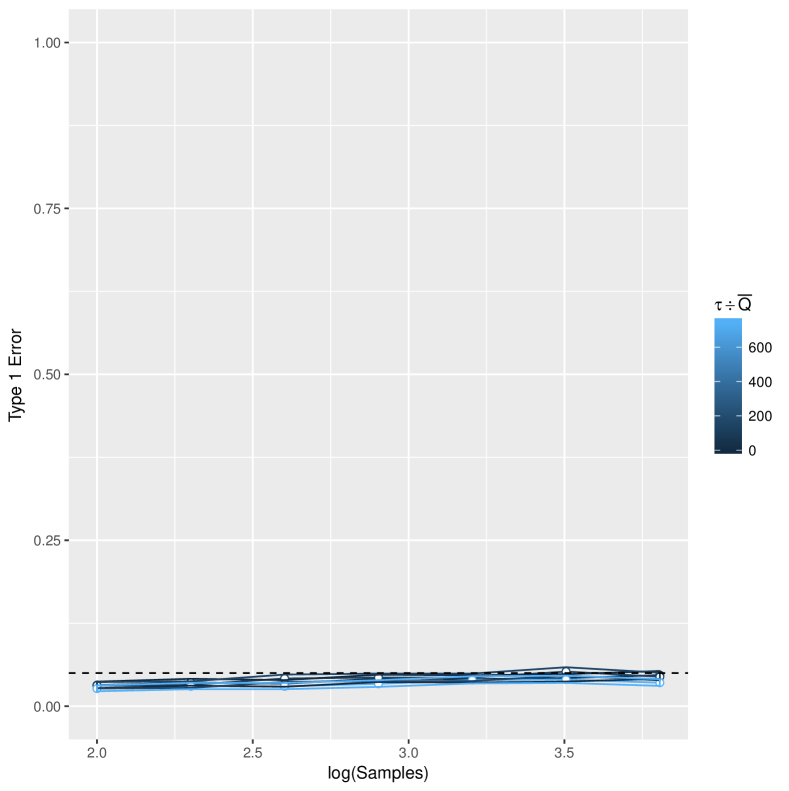
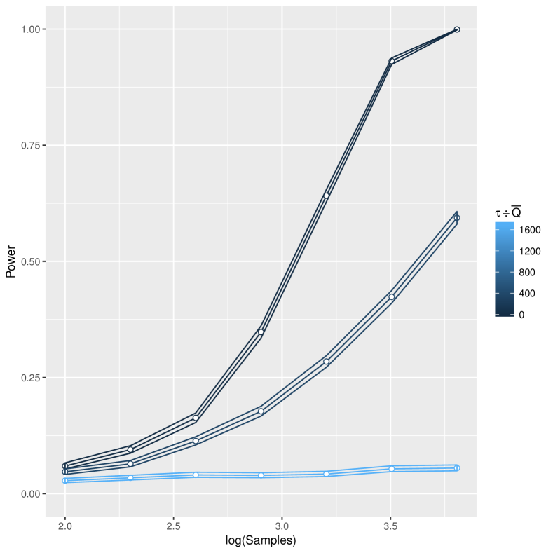
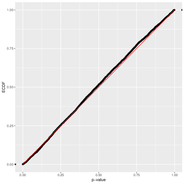
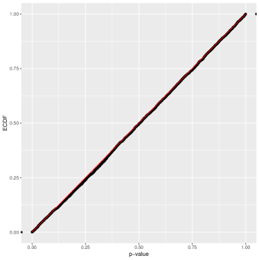
Table 8 presents moment estimates for the distribution of p-values in the null-following case, at various settings of $n$ and $\tau$. For an exact reference distribution under the null hypothesis, the p-values follow the uniform distribution on $[0,1]$, which has mean and variance $0.5,1/12\approx 0.083$ respectively. The results are compatible with a uniform distribution of p-values across a wide range of $n,\tau$, endorsing the assumptions used to derive the reference distribution. Figure 4 depicts the empirical distribution of p-values at $n=6400,\tau=100$, enabling a more detailed assessment of our assumptions.

Figure 4: Rough Pipe Flow p-value empirical CDF with no lurking variables, $n=6400,\tau=100$. Sorted p-values are denoted by dots, with an added red diagonal. The distribution of p-values is approximately uniform, endorsing the choice of reference distribution.

$n$	$\tau$
	$0.00$	$100.00$	$500.00$
$100$	$0.49$, $0.0750$	$0.48$, $0.0736$	$0.47$, $0.0693$
$200$	$0.46$, $0.0747$	$0.47$, $0.0757$	$0.48$, $0.0731$
$400$	$0.49$, $0.0791$	$0.47$, $0.0782$	$0.47$, $0.0710$
$800$	$0.48$, $0.0779$	$0.48$, $0.0813$	$0.47$, $0.0715$
$1600$	$0.49$, $0.0853$	$0.50$, $0.0788$	$0.48$, $0.0756$
$3200$	$0.48$, $0.0830$	$0.50$, $0.0814$	$0.48$, $0.0757$
$6400$	$0.51$, $0.0828$	$0.49$, $0.0801$	$0.49$, $0.0794$

Table 8: Rough Pipe Flow moment estimates of p-value distribution with no lurking variables. Results are presented as pairs of mean, variance. Note that $U(0,1)$ has first moments $0.5$ and $1/12\approx 0.083$. These results suggest that under these conditions, the empirical distribution of p-values is approximately uniform, with the greatest deviations occurring at low sample count and high noise variability.

5.3.2 Two-Fluid Flow

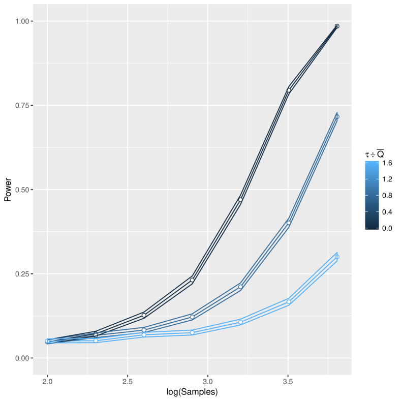
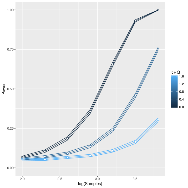
The parameters of the sampling distribution $\boldsymbol{\mu}_{E},\boldsymbol{\Sigma}_{E}$ are chosen to emphasize a large viscosity ratio $\mu_{i}>>\mu_{o}$ and a reasonable range for the other design parameters. We alternately consider the flow variables $\rho,\mu$ as lurking, switching between the inner and outer pairs. Figures 5 and 6 present Type I error and power curves. The right image in Figure 5 demonstrates power indistinguishable from $\alpha=0.05$ at the studied sample counts $n$; this is the case where the inner flow variables are lurking. As noted above, the qoi only weakly depends on these variables, as per engineering design. This example demonstrates that some lurking variables are inherently challenging to detect.

	$\log(\nabla P)$	$\log(h)$	$\log(H)$	$\log(\mu_{o})$	$\log(\mu_{i})$	$\log(\rho_{o})$	$\log(\rho_{i})$
$\boldsymbol{\mu}_{E}$	$1.0397$	$\leavevmode\hphantom{0}\hbox to0.0pt{\hss\leavevmode\resizebox{5.50005pt}{0.0pt}{$-$}}1.7533$	$0.3466$	$0.3466$	$3.8005$	$0.3466$	$1.4979$
$\boldsymbol{\Sigma}_{E}^{1/2}$	$0.3466$	$0.1831$	$0.1155$	$0.1155$	$0.0372$	$0.1155$	$0.0372$

Table 9: Sampling parameters for Two Fluid Flow. The diagonal variance matrix $\boldsymbol{\Sigma}_{E}$ is determined by the given standard deviation components.

Figure 5: Two-Fluid Flow Type I error (left) and power (right). The right image considers a case where the inner viscosity is lurking. This test case demonstrates that some lurking variable are inherently challenging to detect.

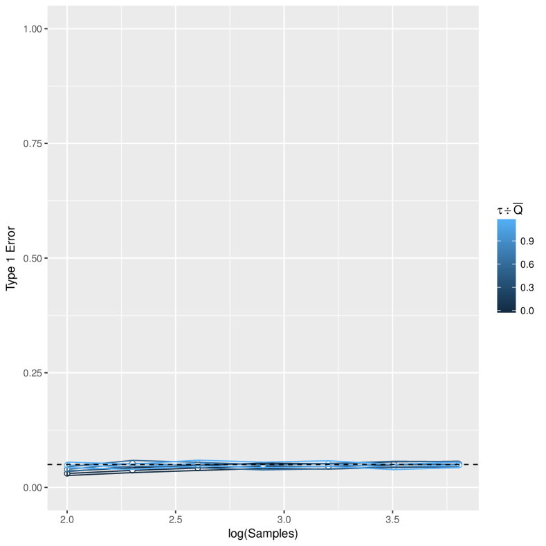
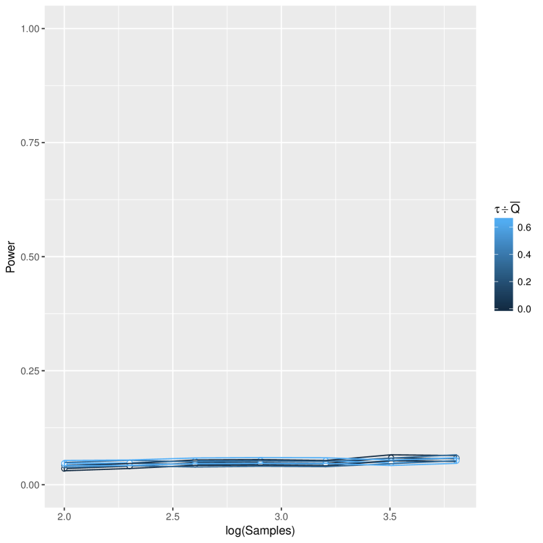
Figure 6 considers cases where the outer viscosity is lurking. The right image considers the inner thickness as a pinned variable, while the left image varies all the exposed variables. Note that the right image necessitates the modified procedure to address the pinned variable. Figure 6 demonstrates that for Two-Fluid Flow and this particular combination of variables, the presence of a pinned variable does not result in a significant power loss. Table 10 presents moment estimates for the distribution of p-values in the case with no lurking variables.

Figure 6: Two-Fluid Flow power without (left) and with (right) pinned variables. Both cases consider the outer viscosity as a lurking variable, while the right additionally considers the inner thickness as a pinned variable. In the cases considered here, the presence of a pinned variable does not result in a significant power loss.

$n$	$\tau$
	$0.00$	$0.50$	$1.00$
$100$	$0.48$, $0.0743$	$0.50$, $0.0820$	$0.51$, $0.0803$
$200$	$0.48$, $0.0832$	$0.48$, $0.0793$	$0.49$, $0.0825$
$400$	$0.47$, $0.0773$	$0.50$, $0.0843$	$0.51$, $0.0838$
$800$	$0.50$, $0.0815$	$0.49$, $0.0831$	$0.49$, $0.0801$
$1600$	$0.51$, $0.0807$	$0.49$, $0.0839$	$0.50$, $0.0807$
$3200$	$0.49$, $0.0799$	$0.49$, $0.0910$	$0.50$, $0.0832$
$6400$	$0.51$, $0.0835$	$0.51$, $0.0829$	$0.51$, $0.0789$

Table 10: Two-Fluid Flow moment estimates of p-value distribution with no lurking variables. These results suggest that under these conditions, the distribution of p-values is uniform.

Figure 7: Two-Fluid Flow p-value empirical CDF with no lurking variables, $n=6400,\tau=0.5$. Sorted p-values are denoted by dots, with an added red diagonal. The distribution of p-values is approximately uniform, endorsing the choice of reference distribution.

As described above, the quantity $\boldsymbol{\nu}$ contains useful information if lurking variables exist. To illustrate, we consider realizations of the sample estimate $\hat{\boldsymbol{\nu}}$ in the two cases considered in Figure 6. For comparison, we compute the quantity $\boldsymbol{W}_{P}\boldsymbol{W}_{P}^{T}\boldsymbol{D}_{L}$ and scale this vector to have the same length as the estimate $\hat{\boldsymbol{\nu}}$; this quantity is reported as $\boldsymbol{w}$. Since there is only one lurking variable in these cases, we expect that $\mathbb{E}[\hat{\boldsymbol{\nu}}]=\boldsymbol{w}$.

Case		M	L	T
Without pinned var	$\hat{\boldsymbol{\nu}}_{L}$	0.8165	-0.9752	-0.7370
	$\boldsymbol{w}_{L}$	0.8487	-0.8487	-0.8487
With pinned var	$\hat{\boldsymbol{\nu}}_{R}$	0.6731	0.0000	-0.6064
	$\boldsymbol{w}_{R}$	0.6406	0.0000	-0.6406

Table 11: Two-Fluid Flow dimension vector estimates. Note that interpreting the dimension vector is relatively straightforward in the case without pinned variables; since the lurking variable is a viscosity, the dimension vector matches the expected $(1,-1,-1)^{T}$, up to a scaling constant. While these results are encouraging, further work is necessary to provide a formal test procedure.

6 Discussion

In this article, we presented a modified form of the Buckingham $\pi$ theorem suitable for testing the presence of lurking variables. We then constructed experimental detection procedures based on a sampling plan informed by Stein’s lemma, a reference distribution arising from Hotelling’s $T^{2}$ test, and reasonable assumptions on the distribution of the response. We supported these assumptions through example problems inspired by engineering applications.

Two points are important to elucidate: the requirements on sampling design, and the sample size requirements for reasonable power. Note that our experimental detection procedure requires that samples be drawn from a Gaussian distribution; this precludes factors which take values at fixed levels. Nonetheless, the potential applications of this approach are myriad, as many physical systems of practical interest feature continuous predictors.

Second, our results suggest that for low sample counts $(n<100)$, the detection power may be unacceptably low $(<0.05)$. To achieve reasonable power, say $0.80$, our numerical experiments suggest that $n>1000$ is necessary for these detection procedures. While sample counts in the thousands are not uncommon for computer experiments, such requirements are beyond a reasonable count for many physical experiments. However, recent advances in microfluidics have enabled kilohertz-throughput experiments which could easily reach our sampling requirements.[1] On the macro-scale, so-called cyber-physical systems enable the automated collection of data, such as $1260$ unique cases of pitching and heaving conditions of an airfoil.[28] Of course, our immediate goal for future work is to reduce the sampling requirements; the intent of the present article is to provide a lucid treatment of detection fundamentals, and to illustrate these principles with minimal assumptions.

Note that in this article, we make relatively modest assumptions on the functional relation between response and predictors. Stein’s lemma may be regarded as implicitly utilizing the smoothness of the response. One could potentially employ stronger assumptions to fruitful ends; namely, increasing power.

Finally, we hope that both the analysis and procedures presented here prove useful to further study. As Albrecht et al.[3] note, Dimensional Analysis is less-studied in the statistics community, and certainly has more untapped potential. We have found the analytical framework presented in Section 2 helpful in reasoning about lurking variables, and hope that others find it similarly useful.

7 Acknowledgments

The authors would like to thank Jessica Hwang and Art Owen for useful comments on the manuscript. The first author would like to thank Arman Sabbaghi for some early comments on this work, and helpful pointers with regard to existing literature. The first author is supported by the National Science Foundation Graduate Research Fellowship under Grant No. DGE-114747. The second author was supported by the NSF under Grants No. DMS-1407397 and DMS-1521145.

8 Appendix

Remark (Unit Systems).

There is historical precedent for changing unit systems; the 1875 Treaty of the Metre established a standard unit of length based on a prototype metre, kept in controlled conditions. This was redefined again in 1960 in terms of the krypton-86 spectrum, to avoid the obvious issues of such a prototype definition.[26] The meter was redefined several times since, and now is based on the distance light travels in a vacuum in $1/299,792,458$ seconds.[27]

8.1 Unique non-dimensionalizing factor

Suppose we have some dimensional qoi $q$. We may form a dimensionless qoi $\pi$ by constructing a non-dimensionalizing factor as a power-product of the input quantities $\boldsymbol{z}$. Such a non-dimensionalizing factor satisfies $[\prod_{i=1}^{p}z_{i}^{u_{i}}]=[q]$. Having found such a non-dimensionalizing vector $\boldsymbol{u}\in\mathbb{R}^{p}$, we may form

$$\pi=q\prod_{i=1}^{p}z_{i}^{-u_{i}}=q\exp(-\boldsymbol{u}^{T}\log(\boldsymbol{z})).$$

Dimensional homogeneity demands that $\boldsymbol{d}(q)\in\mathcal{R}(\boldsymbol{D})$, thus a non-dimensionalizing factor always exists. However, an analyst may not be aware of the full $\boldsymbol{z}$, and may know only of the exposed variables $\boldsymbol{z}_{E}$. A non-dimensionalizing vector $\boldsymbol{u}_{E}$ may not exist for the exposed factors, and is not necessarily unique. As Bridgman [7] notes, one must have $\boldsymbol{d}(q)\in\mathcal{R}(\boldsymbol{D}_{E})$ in order for dimensional homogeneity to hold. Below we prove existence and uniqueness of a particular $\boldsymbol{u}_{E}$ under this condition.

Theorem 1 (Existence of a unique non-dimensionalizing factor).

If a physical relationship is dimensionally homogeneous in the full $\boldsymbol{z}$, and some $\boldsymbol{z}_{E}$ are known with $\boldsymbol{d}(q)\in\mathcal{R}(\boldsymbol{D}_{E})$, there exists a unique non-dimensionalizing vector $\boldsymbol{u}_{E}^{*}\in\mathbb{R}^{p_{E}}$ for the qoi $q$ that is orthogonal to the nullspace of $\boldsymbol{D}_{E}$.

Proof of Theorem 1.

Since $\boldsymbol{d}(q)\in\mathcal{R}(\boldsymbol{D}_{E})$, we know a solution to $\boldsymbol{D}_{E}\boldsymbol{u}_{E}=\boldsymbol{d}(q)$ exists. Denote $r_{E}=\text{Rank}(\boldsymbol{D}_{E})$. Employing the Rank-Nullity theorem, let $\boldsymbol{V}_{E}\in\mathbb{R}^{p_{E}\times(p_{E}-r_{E})}$ be a basis for $\text{Null}(\boldsymbol{D}_{E})$. Define the matrix

$$\boldsymbol{M}=\left[\begin{array}[]{c}\boldsymbol{D}_{E}\\ \boldsymbol{V}_{E}^{T}\end{array}\right],$$ (32)

and note that $\boldsymbol{M}\in\mathbb{R}^{(d+p_{E}-r_{E})\times p_{E}}$. Define the vector $\boldsymbol{b}\in\mathbb{R}^{(d+p_{E}-r_{E})}$ via $\boldsymbol{b}^{T}=[\boldsymbol{d}(q)^{T},\boldsymbol{0}^{T}]$, where $\boldsymbol{0}\in\mathbb{R}^{p_{E}-r_{E}}$. Then the solution to the linear system $\boldsymbol{M}\boldsymbol{u}_{E}=\boldsymbol{b}$ is a non-dimensionalizing vector for $q$, and is orthogonal to the nullspace of $\boldsymbol{D}_{E}$.

Note that $\boldsymbol{d}(q)\in\mathcal{R}(\boldsymbol{D}_{E})$ and $\boldsymbol{0}\in\mathcal{R}(\boldsymbol{V}_{E}^{T})$, thus the augmented matrix $[\boldsymbol{M}|\boldsymbol{b}]$ has the property $\text{Rank}(\boldsymbol{M})=\text{Rank}([\boldsymbol{M}|\boldsymbol{b}])$. Note also that there are $r_{E}$ independent rows in $\boldsymbol{D}_{E}$ and $p_{E}-r_{E}$ independent rows in $\boldsymbol{V}_{E}^{T}$, with $\boldsymbol{D}_{E}\boldsymbol{V}_{E}=0$. Thus we have $\text{Rank}(\boldsymbol{M})=p_{E}$. By the Rouché-Capelli theorem, we know that a solution $\boldsymbol{u}_{E}^{*}$ to $\boldsymbol{M}\boldsymbol{u}_{E}=\boldsymbol{b}$ exists and is unique. ∎

References

- [1] A. R. Abate, T. Hung, P. Mary, J. J. Agresti, and D. A. Weitz, High-throughput injection with microfluidics using picoinjectors, Proceedings of the National Academy of Sciences, 107 (2010), pp. 19163–19166.
- [2] K. P. Adragni and R. D. Cook, Sufficient dimension reduction and prediction in regression, Philosophical Transactions of the Royal Society of London A: Mathematical, Physical and Engineering Sciences, 367 (2009), pp. 4385–4405.
- [3] M. C. Albrecht, C. J. Nachtsheim, T. A. Albrecht, and R. D. Cook, Experimental design for engineering dimensional analysis, Technometrics, 55 (2013), pp. 257–270, https://doi.org/10.1080/00401706.2012.746207, http://dx.doi.org/10.1080/00401706.2012.746207, https://arxiv.org/abs/http://dx.doi.org/10.1080/00401706.2012.746207.
- [4] T. W. Anderson, An introduction to multivariate statistical analysis, vol. 2, Wiley New York, 1958.
- [5] G. I. Barenblatt, Scaling, self-similarity, and intermediate asymptotics: dimensional analysis and intermediate asymptotics, Cambridge University Press, 1996.
- [6] G. E. P. Box, Use and abuse of regression, Technometrics, 8 (1966), pp. 625–629, http://www.jstor.org/stable/1266635.
- [7] P. W. Bridgman, Dimensional analysis, Yale University Press, 1922.
- [8] E. Buckingham, On physically similar systems; illustrations of the use of dimensional equations, Phys. Rev., 4 (1914), pp. 345–376, https://doi.org/10.1103/PhysRev.4.345, http://link.aps.org/doi/10.1103/PhysRev.4.345.
- [9] C. Colebrook and C. White, Experiments with fluid friction in roughened pipes, Proceedings of the Royal Society of London. Series A, Mathematical and Physical Sciences, 161 (1937), pp. 367–381, http://www.jstor.org/stable/96790.
- [10] P. G. Constantine, Z. del Rosario, and G. Iaccarino, Many physical laws are ridge functions, ArXiv e-prints, (2016), https://arxiv.org/abs/1605.07974.
- [11] G. Csárdi and R. FitzJohn, progress: Terminal Progress Bars, 2016, https://CRAN.R-project.org/package=progress. R package version 1.1.2.
- [12] Z. del Rosario, P. G. Constantine, and G. Iaccarino, Developing design insight through active subspaces, in 19th AIAA Non-Deterministic Approaches Conference, 2017, p. 1090.
- [13] S. Dorai-Raj, binom: Binomial Confidence Intervals For Several Parameterizations, 2014, https://CRAN.R-project.org/package=binom. R package version 1.1-1.
- [14] B. L. Joiner, Lurking variables: Some examples, The American Statistician, 35 (1981), pp. 227–233.
- [15] T. Kariya, A robustness property of hotelling’s t2-test, The Annals of Statistics, (1981), pp. 211–214.
- [16] E. L. Lehmann and G. Casella, Theory of point estimation, Springer Science & Business Media, 2006.
- [17] K. V. Mardia, Assessment of multinormality and the robustness of hotelling’s test, Applied Statistics, (1975), pp. 163–171.
- [18] J. Nikuradse, Laws of flow in rough pipes, (1950).
- [19] A. C. Palmer, Dimensional analysis and intelligent experimentation, World Scientific Publishing Co Inc, 2008.
- [20] J. Pearl and E. Bareinboim, External validity: From do-calculus to transportability across populations, Statistical Science, 29 (2014), pp. 579–595.
- [21] R Core Team, R: A Language and Environment for Statistical Computing, R Foundation for Statistical Computing, Vienna, Austria, 2017, https://www.R-project.org/.
- [22] O. Reynolds, An experimental investigation of the circumstances which determine whether the motion of water shall be direct or sinuous, and of the law of resistance in parallel channels., Proceedings of the royal society of London, 35 (1883), pp. 84–99.
- [23] W. Shen and D. K. J. Lin, A conjugate model for dimensional analysis, Technometrics, 0 (2017), pp. 1–11, https://doi.org/10.1080/00401706.2017.1291451, http://dx.doi.org/10.1080/00401706.2017.1291451, https://arxiv.org/abs/http://dx.doi.org/10.1080/00401706.2017.1291451.
- [24] A. A. Sonin, The physical basis of dimensional analysis, 2001.
- [25] C. M. Stein, Estimation of the mean of a multivariate normal distribution, The annals of Statistics, (1981), pp. 1135–1151.
- [26] The Editors of Encyclopædia Britannica, Metric system, https://www.britannica.com/science/metric-system-measurement#ref258582.
- [27] A. Thompson and B. N. Taylor, Guide for the use of the international system of units (si), tech. report, 2008.
- [28] T. Van Buren, D. Floryan, and A. J. Smits, Scaling and performance of simultaneously heaving and pitching airfoils, AIAA Journal, (Forthcoming).
- [29] W. N. Venables and B. D. Ripley, Modern Applied Statistics with S, Springer, New York, fourth ed., 2002, http://www.stats.ox.ac.uk/pub/MASS4. ISBN 0-387-95457-0.
- [30] F. M. White, Fluid Mechanics, McGraw-Hill, New York, 2011.
- [31] H. Wickham, ggplot2: Elegant Graphics for Data Analysis, Springer-Verlag New York, 2009, http://ggplot2.org.
- [32] E. B. Wilson, Probable inference, the law of succession, and statistical inference, Journal of the American Statistical Association, 22 (1927), pp. 209–212.