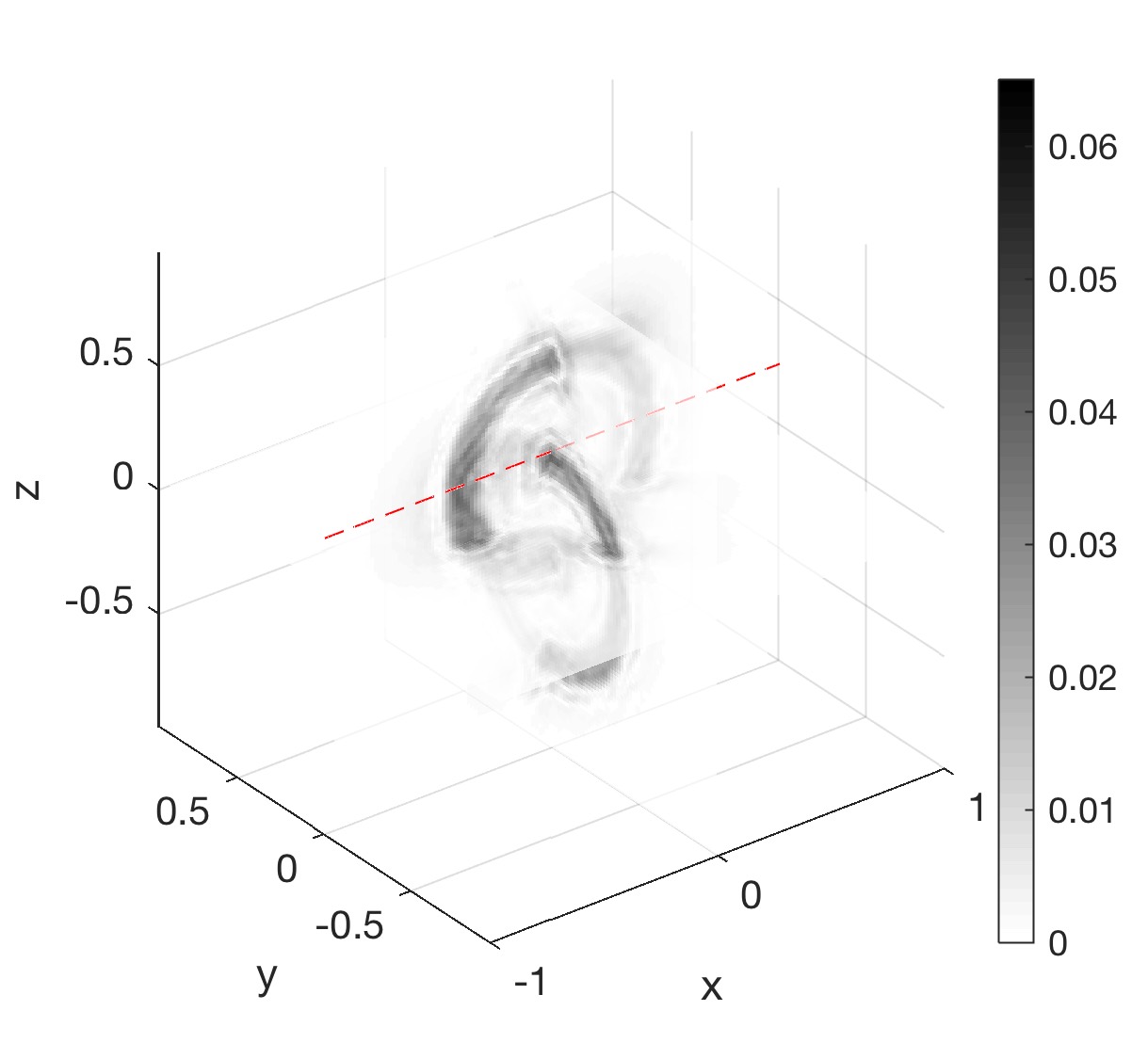
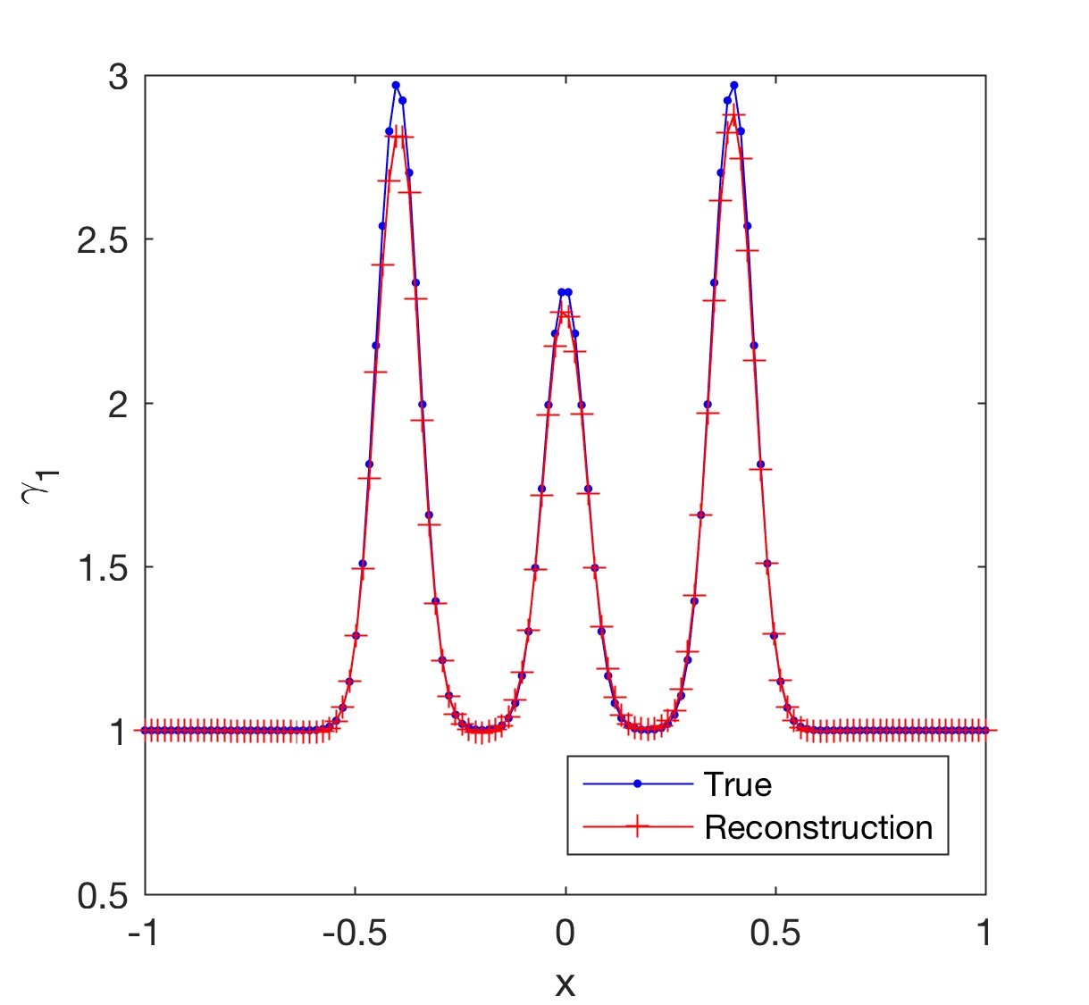
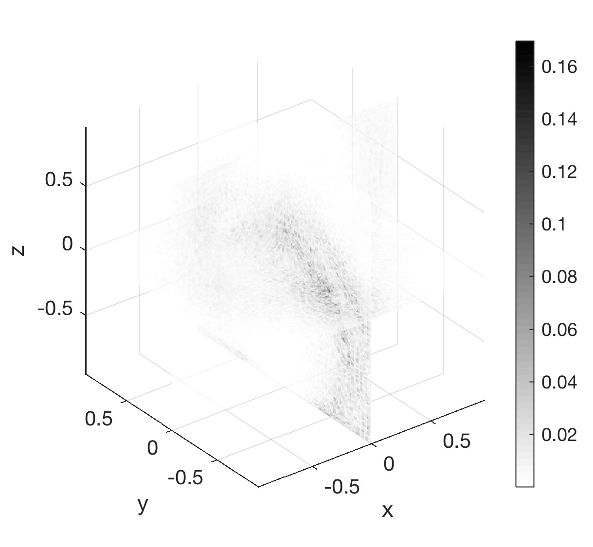
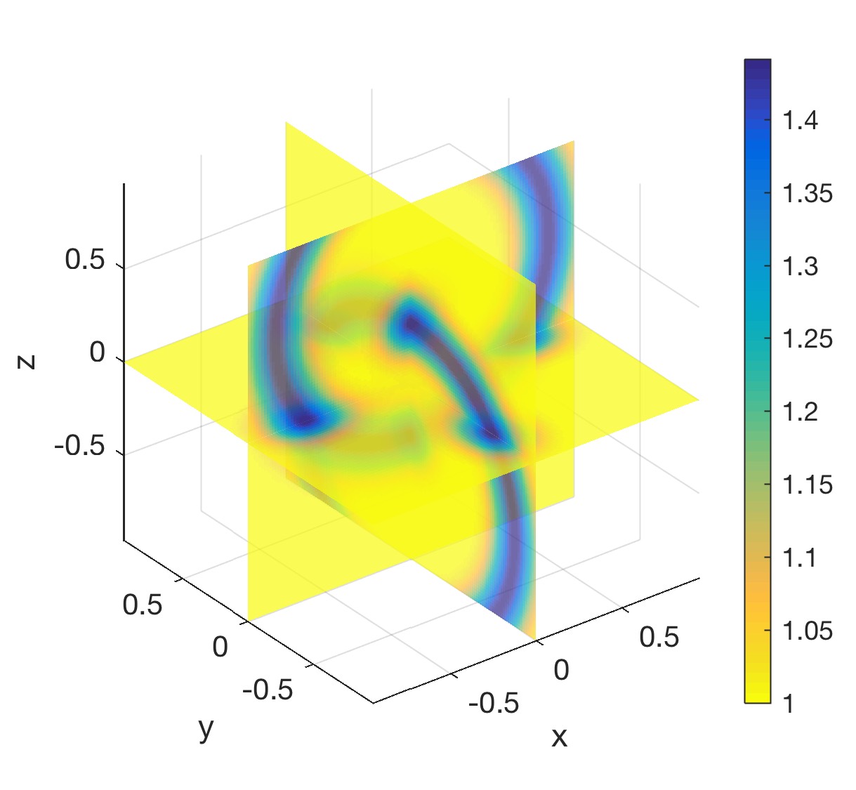
Imaging of isotropic and anisotropic conductivities from power densities in three dimensions

François Monard Department of Mathematics, University of California, Santa Cruz CA 95064, USA. fmonard@ucsc.edu    Donsub Rim Department of Applied Physics and Applied Mathematics, Columbia University, New York NY, USA. dr2965@columbia.edu
Abstract

We present numerical reconstructions of anisotropic conductivity tensors in three dimensions, from knowledge of a finite family of power density functionals. Such a problem arises in the coupled-physics imaging modality Ultrasound Modulated Electrical Impedance Tomography for instance. We improve on the algorithms previously derived in [9, 32] for both isotropic and anisotropic cases, and we address the well-known issue of vanishing determinants in particular. The algorithm is implemented and we provide numerical results that illustrate the improvements.

1 Introduction

We present a numerical implementation of reconstruction algorithms previously derived in [9, 32] for isotropic and anisotropic conductivity tensors in three spatial dimensions, from knowledge of a finite number of so-called power density measurements. Put in mathematical terms, the problem considered is to reconstruct γ:XS3():𝛾𝑋subscript𝑆3\gamma:X\to S_{3}(\mathbb{R}) a symmetric, uniformly elliptic111γ𝛾\gamma is uniformly elliptic if there exists a constant κ1𝜅1\kappa\geq 1 such that κ1|ξ|2γ(x)ξξκ|ξ|2superscript𝜅1superscript𝜉2𝛾𝑥𝜉𝜉𝜅superscript𝜉2\kappa^{-1}|\xi|^{2}\leq\gamma(x)\xi\cdot\xi\leq\kappa|\xi|^{2} for every xX𝑥𝑋x\in X and ξ3𝜉superscript3\xi\in\mathbb{R}^{3}. conductivity tensor on a given bounded domain X3𝑋superscript3X\subset\mathbb{R}^{3} from the knowledge of a finite collection of internal functionals of the form Hij(x)=γ(x)ui(x)uj(x)subscript𝐻𝑖𝑗x𝛾xsubscript𝑢𝑖xsubscript𝑢𝑗xH_{ij}({\mathrm{x}})=\gamma({\mathrm{x}})\nabla u_{i}({\mathrm{x}})\cdot\nabla u_{j}({\mathrm{x}}) for 1i,jJformulae-sequence1𝑖𝑗𝐽1\leq i,j\leq J, where each uisubscript𝑢𝑖u_{i} solves the conductivity equation

(γui)=0(in X),u|X=gi(prescribed).formulae-sequence𝛾subscript𝑢𝑖0in 𝑋evaluated-at𝑢𝑋subscript𝑔𝑖prescribed\displaystyle\nabla\cdot(\gamma\nabla u_{i})=0\qquad(\text{in }X),\qquad u|_{\partial X}=g_{i}\quad(\text{prescribed}). (1)

The inverse conductivity problem from power densities belongs to the family of hybrid (or coupled-physics) inverse problems, whose primary purpose is to design high-contrast, high-resolution medical imaging modalities by coupling two traditional imaging techniques with complementary strengths [5, 7].

Two examples of hybrid models couple conductivity imaging with ultrasonic waves, one so-called Impedance Acoustic Tomography [24], and the other, Ultrasound-Modulated Electrical Impedance Tomography [4]. These modalities ultimately lead to an inverse problem where one is provided with internal functionals (even though the method remains non-invasive) to reconstruct the internal, anisotropic conductivity. Such a problem has received much attention over the past few years, both in theoretical and numerical aspects [21, 9, 13, 26, 32, 30, 31, 10, 15, 3, 17]. In particular, the first author’s prior work on the topic has consisted of the derivation of explicit reconstruction algorithms for the non-linear problem in all dimensions d2𝑑2d\geq 2, and the analysis of their stability. These results serve as a justification that power density measurements show much promise in their ability to give access to conductivities at higher resolution than from classical Dirichlet-to-Neumann data, and furthermore give access to anisotropic features which are traditionally unavailable in the classical Calderón’s problem.

Inverse conductivity problems share many similarities with inverse elasticity problems [8, 27, 14, 23], and some of the current framework also applies there as well, see [14]. Other internal functionals for inverse conductivity may be considered, for instance current densities, see [22, 38, 36, 35, 12, 11, 34].

Implementations often use iterative methods as in [4, 15, 25], for which finding a good initial guess can be crucial. The approach presented here consists in implementing explicit inversion algorithms, which may either provide satisfactory reconstructions in some cases, or a good initial guess for further improvements in others. Previous implementations in two dimensions were presented in [30] and we now present a three-dimensional implementation. In this problem, the transition from two to three spatial dimensions requires additional technical considerations, even if one ignores the issue of computational cost.

  • In the isotropic case where one must reconstruct a function R:XSO(3):𝑅𝑋𝑆𝑂3R:X\to SO(3) by integration of a dynamical system along curves, a choice needs to be made on how to parameterize SO(3)𝑆𝑂3SO(3), involving a number of parameters between 333 and 999. Too few parameters (3: the Euler angles) lead to singularity issues not due to the actual problem but to the parameterization, see [37]; too many parameters (9, the full matrix) increases redundancy, computational cost and complexity of the dynamical system to be integrated. In this article, we use unit quaternions {\mathbb{H}}, a 444-parameter family describing SO(3)𝑆𝑂3SO(3) non-singularly. This description gives a good dimensionality tradeoff, moreover computations below show that the dynamical system parameterized in that way admits a rather symmetric form, easier to implement than the previously derived system for the 999-parameter rotation matrix. While the correspondence SO(3)𝑆𝑂3{\mathbb{H}}\to SO(3) is 2-to-1, this is the price to pay for using a non-singular parameterization of SO(3)𝑆𝑂3SO(3), and in fact does not cause specific issues in the implementation.

  • The validity of the reconstruction algorithms comes with conditions on the boundary conditions gisubscript𝑔𝑖g_{i}, which are easy to satisfy in two dimensions, much less obvious in three [1, 20, 10]. In particular, two issues associated with this are: (i) how to find boundary conditions satisfying the validity conditions; (ii) if more than the minimal number of solutions is needed, how does one efficiently determine which set works locally, and how does one combine the local reconstructions into a global one ? While (i) is a difficult theoretical question which continues to receive attention and is not the focus of the present article, we address (ii) as follows: in [9], it was suggested to decompose the domain and patch local reconstructions together, but we will give a way to do this globally at once, allowing for more efficiency in the reconstruction process.

Outline.

We first present in Section 2 a summary of the problems considered, their dimension and the existing approaches, before discussing in Section 3 the derivation of a reconstruction algorithm in the isotropic case, making use of quaternion algebra. We then adapt in Section 4 the reconstruction algorithms for anisotropic tensors to three dimensions. The numerical simulations are presented in Section 5, and some concluding remarks are provided in Section 6.

2 Summary of problems considered and existing approaches

We briefly recall the results from [9, 31, 30, 32, 13, 29], and we will build upon them. The analysis there consists in finding a minimal set of functionals for which reconstructions algorithms can be derived, with stability estimates in optimal spaces. For such analyses, it is natural to consider decomposing an anisotropic conductivity γ𝛾\gamma into the product γ=τγ~𝛾𝜏~𝛾\gamma=\tau\tilde{\gamma} with τ𝜏\tau a scalar function and γ~~𝛾\tilde{\gamma} a tensor satisfying detγ~=1~𝛾1\det\tilde{\gamma}=1. Then the following three settings have been considered.

(1) Reconstruction of an isotropic (γ~=Id~𝛾𝐼𝑑\tilde{\gamma}=Id) conductivity. τ𝜏\tau is usually denoted σ𝜎\sigma in this case.

(1’) In the anisotropic case, reconstruction of the scalar τ𝜏\tau assuming knowledge of γ~~𝛾\tilde{\gamma}.

(2) In the anisotropic case, reconstruction of γ~~𝛾\tilde{\gamma}, then τ𝜏\tau.

Problem (1’) is a generalization of Problem (1), of same dimensionality and resolution approach. Incorporating the presence of a non-trivial γ~~𝛾\tilde{\gamma} to solve (1’) is addressed in [32, Sec. 3.1] and will not be further addressed in the present article.

2.1 Local reconstruction algorithms

We recall the results in any dimension n2𝑛2n\geq 2.

Local resolution of Problem (1).

See, e.g., [9, 31]. Suppose XXsuperscript𝑋𝑋X^{\prime}\subset X and assume that n𝑛n solutions u1,,unsubscript𝑢1subscript𝑢𝑛u_{1},\dots,u_{n} of (1) (with associated power densities {Hij}1ijnsubscriptsubscript𝐻𝑖𝑗1𝑖𝑗𝑛\{H_{ij}\}_{1\leq i\leq j\leq n}) satisfy

infxXdet(u1(x),,un(x))c0>0.subscriptinfimumxsuperscript𝑋subscript𝑢1xsubscript𝑢𝑛xsubscript𝑐00\displaystyle\inf_{{\mathrm{x}}\in X^{\prime}}\det(\nabla u_{1}({\mathrm{x}}),\dots,\nabla u_{n}({\mathrm{x}}))\geq c_{0}>0. (2)

Then one may reconstruct σ|Xevaluated-at𝜎superscript𝑋\sigma|_{X^{\prime}} in Problem (1) up to a constant, from {Hij|X}1ijnsubscriptevaluated-atsubscript𝐻𝑖𝑗superscript𝑋1𝑖𝑗𝑛\{H_{ij}|_{X^{\prime}}\}_{1\leq i\leq j\leq n} with a W1,W1,superscript𝑊1superscript𝑊1W^{1,\infty}\to W^{1,\infty} stability estimate, see [31, Theorem 2.3]. In a nutshell, the quantities u1,,unsubscript𝑢1subscript𝑢𝑛\nabla u_{1},\dots,\nabla u_{n} are known from data up to an unknown rotation matrix R:ΩSO(n):𝑅Ω𝑆𝑂𝑛R:\Omega\to SO(n), and the approach consists in deriving explicit equations for the full gradients logσ𝜎\nabla\log\sigma and R𝑅\nabla R as functions of R𝑅R and the known data. Such equations then turn into dynamical systems along any desired integration curve, allowing the reconstruction of σ𝜎\sigma along a family of curves covering Xsuperscript𝑋X^{\prime}, see Section 3 for details. An alternate reconstruction approach was also proposed in [31, Section 5] involving solving a coupled elliptic system, not covered further here.

Local resolution of Problem (2).

See, e.g., [30, 32, 13]. To address Problem (2), a family (u1,,un)subscript𝑢1subscript𝑢𝑛(u_{1},\dots,u_{n}) satisfying (2) needs to be augmented with additional solutions, call them (v1,,vm)subscript𝑣1subscript𝑣𝑚(v_{1},\dots,v_{m}), with m𝑚m to be determined. For each additional solution vjsubscript𝑣𝑗v_{j}, the power densities {γuivj}i=1nsuperscriptsubscript𝛾subscript𝑢𝑖subscript𝑣𝑗𝑖1𝑛\{\gamma\nabla u_{i}\cdot\nabla v_{j}\}_{i=1}^{n} can be exploited to bring potentially 1+n(n1)/21𝑛𝑛121+n(n-1)/2 pointwise linear constraints on γ~~𝛾\tilde{\gamma} in the form “tr (Mjp(x)γ~(x))=0tr subscript𝑀𝑗𝑝x~𝛾x0\text{tr }(M_{jp}({\mathrm{x}})\tilde{\gamma}({\mathrm{x}}))=0”, where {Mjp(x)}p=11+n(n1)/2superscriptsubscriptsubscript𝑀𝑗𝑝x𝑝11𝑛𝑛12\{M_{jp}({\mathrm{x}})\}_{p=1}^{1+n(n-1)/2} are matrices known from power densities. If m𝑚m is then chosen large enough, and if the family

{Mjp(x),1jm,1p1+n(n1)/2}formulae-sequencesubscript𝑀𝑗𝑝x1𝑗𝑚1𝑝1𝑛𝑛12\left\{M_{jp}({\mathrm{x}}),\quad 1\leq j\leq m,\quad 1\leq p\leq 1+n(n-1)/2\right\}

spans the hyperplane {γ~(x)}superscript~𝛾xperpendicular-to\{\tilde{\gamma}({\mathrm{x}})\}^{\perp} of dimension n21superscript𝑛21n^{2}-1 in Mn()subscript𝑀𝑛M_{n}(\mathbb{R}) at every point of Xsuperscript𝑋X^{\prime}, then one may reconstruct γ~~𝛾\tilde{\gamma} pointwise by choosing a normal to that hyperplane. Such reconstructibility conditions can be formulated as a constraint of the form

infxX𝒫({Hij(x),Hij(x)}1ijn+m)c>0,subscriptinfimumxsuperscript𝑋𝒫subscriptsubscript𝐻𝑖𝑗xsubscript𝐻𝑖𝑗x1𝑖𝑗𝑛𝑚𝑐0\displaystyle\inf_{{\mathrm{x}}\in X^{\prime}}{\cal P}(\{H_{ij}({\mathrm{x}}),\nabla H_{ij}({\mathrm{x}})\}_{1\leq i\leq j\leq n+m})\geq c>0, (3)

with 𝒫𝒫{\cal P} a polynomial, see [32, Eq. (11)]. When (3) is satisfied, then γ~|Xevaluated-at~𝛾superscript𝑋\tilde{\gamma}|_{X^{\prime}} can be reconstructed pointwise, with Lsuperscript𝐿L^{\infty} norm stably controlled by the W1,superscript𝑊1W^{1,\infty} norm of the power densities, as proved in [32, Theorem 2.7]. Note that this loss of one derivative was shown to be optimal in [13]. Once γ~~𝛾\tilde{\gamma} is reconstructed τ𝜏\tau can in turn be reconstructed, either as in Problem (1’) (involving a dynamical approach similar to Problem (1)), or more directly as the additional data also allows for more efficient reconstruction of τ𝜏\tau (i.e., no dynamical system required), see Section 4 for details.

Now considering the case n=3𝑛3n=3, we see that the reconstructibility condition (3) can in principle be satisfied with only 222 additional solutions (since they generate 8 orthogonality constraints in a 9-dimensional space), hence the name of 3+2323+2 algorithm in Section 4.2 below.

2.2 From local to global

In light of these local algorithms, one may wonder whether conditions (2) and (3) can hold globally on X𝑋X by choosing appropriate solutions (u1,,un,v1,,vm)subscript𝑢1subscript𝑢𝑛subscript𝑣1subscript𝑣𝑚(u_{1},\dots,u_{n},v_{1},\dots,v_{m}). The answer to this question is well-understood and positive in two dimensions [2]. In higher dimensions, it holds in a few cases including tensors close enough to constant (see [32, Theorem 2.8]), yet the question is generally open, including counterexamples [1, 20, 21]. Thus in three dimensions, it is currently more reasonable to think of a strategy which patches together local reconstructions, by covering X𝑋X with open subdomains X1,,XNsubscript𝑋1subscript𝑋𝑁X_{1},\dots,X_{N} and finding solutions satisfying conditions (2) and (3) on each Xjsubscript𝑋𝑗X_{j} which guarantee reconstructibility of γ𝛾\gamma on each Xjsubscript𝑋𝑗X_{j}. That such a scenario is possible can be proved under mild regularity assumptions on γ𝛾\gamma and the Runge approximation property (see [32, Theorem 2.5]).

A first patching approach was first described in [9, Section 5.2], requiring to keep track of (i) the covering, and (ii) which set of solutions satisfies conditions (2)-(3) on which subdomain. We derive an approach below which does not require keeping track of such a covering explicitly, and derives global equations to reconstruct the unknowns all at once. Such an approach implicitly exploits the fact that, given a family of solutions, conditions (2) and (3) hold locally for some subfamily of these solutions. See Section 4.3 for detail.

3 Isotropic reconstructions from 333 solutions

We now recall the derivation of the reconstruction for the isotropic case, following, e.g., [9]. Consider the reconstruction of a scalar conductivity σ𝜎\sigma from knowledge of power densities Hij=σuiujsubscript𝐻𝑖𝑗𝜎subscript𝑢𝑖subscript𝑢𝑗H_{ij}=\sigma\nabla u_{i}\cdot\nabla u_{j} for 1i,j3formulae-sequence1𝑖𝑗31\leq i,j\leq 3 corresponding to three solutions

(σuj)=0(in X),uj|X=gj(prescribed),1j3,formulae-sequence𝜎subscript𝑢𝑗0in 𝑋formulae-sequenceevaluated-atsubscript𝑢𝑗𝑋subscript𝑔𝑗(prescribed)1𝑗3\displaystyle\nabla\cdot(\sigma\nabla u_{j})=0\qquad(\text{in }X),\qquad u_{j}|_{\partial X}=g_{j}\quad\text{(prescribed)},\qquad 1\leq j\leq 3,

such that (u1,u2,u3)subscript𝑢1subscript𝑢2subscript𝑢3(\nabla u_{1},\nabla u_{2},\nabla u_{3}) is linearly independent at every point of an open subset ΩXΩ𝑋\Omega\subset X. Define Si:=σuiassignsubscript𝑆𝑖𝜎subscript𝑢𝑖S_{i}:=\sqrt{\sigma}\nabla u_{i}, 1i31𝑖31\leq i\leq 3, whose inner products are known since Hij=Si,Sjsubscript𝐻𝑖𝑗subscript𝑆𝑖subscript𝑆𝑗H_{ij}=\left\langle S_{i},S_{j}\right\rangle, and satisfy the PDEs

Si+FSi=0,×SiF×Si=0,F:=12logσ,1i3.formulae-sequencesubscript𝑆𝑖𝐹subscript𝑆𝑖0formulae-sequencesubscript𝑆𝑖𝐹subscript𝑆𝑖0formulae-sequenceassign𝐹12𝜎1𝑖3\displaystyle\nabla\cdot S_{i}+F\cdot S_{i}=0,\qquad\nabla\times S_{i}-F\times S_{i}=0,\qquad F:=\frac{1}{2}\nabla\log\sigma,\qquad 1\leq i\leq 3.

Let S𝑆S be the M3()subscript𝑀3M_{3}(\mathbb{R})-valued matrix with colums (S1,S2,S3)subscript𝑆1subscript𝑆2subscript𝑆3(S_{1},S_{2},S_{3}). Executing a QR decomposition on S𝑆S, we define an SO(3)𝑆𝑂3SO(3)-valued function R=STT𝑅𝑆superscript𝑇𝑇R=ST^{T}, with transition matrix (known from power densities)

T={tij}1i,j3=[H111200H12H1112d1H1112d10(H12H23H22H13)(dD)1(H12H13H11H23)(dD)1dD1]𝑇subscriptsubscript𝑡𝑖𝑗formulae-sequence1𝑖𝑗3delimited-[]superscriptsubscript𝐻111200subscript𝐻12superscriptsubscript𝐻1112superscript𝑑1superscriptsubscript𝐻1112superscript𝑑10subscript𝐻12subscript𝐻23subscript𝐻22subscript𝐻13superscript𝑑𝐷1subscript𝐻12subscript𝐻13subscript𝐻11subscript𝐻23superscript𝑑𝐷1𝑑superscript𝐷1\displaystyle T=\{t_{ij}\}_{1\leq i,j\leq 3}=\left[\begin{array}[]{ccc}H_{11}^{-\frac{1}{2}}&0&0\\ -H_{12}H_{11}^{-\frac{1}{2}}d^{-1}&H_{11}^{\frac{1}{2}}d^{-1}&0\\ (H_{12}H_{23}-H_{22}H_{13})(dD)^{-1}&(H_{12}H_{13}-H_{11}H_{23})(dD)^{-1}&dD^{-1}\end{array}\right]

with d:=(H11H22H122)12assign𝑑superscriptsubscript𝐻11subscript𝐻22superscriptsubscript𝐻12212d:=(H_{11}H_{22}-H_{12}^{2})^{\frac{1}{2}} and D=(detH)12𝐷superscript𝐻12D=(\det H)^{\frac{1}{2}}. Denoting tijsuperscript𝑡𝑖𝑗t^{ij} the entries of T1superscript𝑇1T^{-1}, we further define for 1i,k3formulae-sequence1𝑖𝑘31\leq i,k\leq 3

Vik:=(tij)tjk,Viks=12(Vik+Vki),Vika:=12(VikVki).formulae-sequenceassignsubscript𝑉𝑖𝑘subscript𝑡𝑖𝑗superscript𝑡𝑗𝑘formulae-sequencesuperscriptsubscript𝑉𝑖𝑘𝑠12subscript𝑉𝑖𝑘subscript𝑉𝑘𝑖assignsuperscriptsubscript𝑉𝑖𝑘𝑎12subscript𝑉𝑖𝑘subscript𝑉𝑘𝑖\displaystyle V_{ik}:=(\nabla t_{ij})t^{jk},\qquad V_{ik}^{s}=\frac{1}{2}(V_{ik}+V_{ki}),\qquad V_{ik}^{a}:=\frac{1}{2}(V_{ik}-V_{ki}). (4)

Then the PDEs for (S1,S2,S3)subscript𝑆1subscript𝑆2subscript𝑆3(S_{1},S_{2},S_{3}) may turn into PDEs for (R1,R2,R3)subscript𝑅1subscript𝑅2subscript𝑅3(R_{1},R_{2},R_{3}), the columns of the R𝑅R matrix, given by

Ri=VikRkFRi,×Ri=Vik×Rk+F×Ri,i=1,2,3.formulae-sequencesubscript𝑅𝑖subscript𝑉𝑖𝑘subscript𝑅𝑘𝐹subscript𝑅𝑖formulae-sequencesubscript𝑅𝑖subscript𝑉𝑖𝑘subscript𝑅𝑘𝐹subscript𝑅𝑖𝑖123\displaystyle\nabla\cdot R_{i}=V_{ik}\cdot R_{k}-F\cdot R_{i},\qquad\nabla\times R_{i}=V_{ik}\times R_{k}+F\times R_{i},\qquad i=1,2,3.

Out of this system, we derive in [9, Eq. (18)] the equation

F=12logσ=16logdetH+23Vijs,RiRj,𝐹12𝜎16𝐻23superscriptsubscript𝑉𝑖𝑗𝑠subscript𝑅𝑖subscript𝑅𝑗\displaystyle F=\frac{1}{2}\nabla\log\sigma=\frac{1}{6}\nabla\log\det H+\frac{2}{3}\left\langle V_{ij}^{s},R_{i}\right\rangle R_{j}, (5)

as well as, for m,i=1,2,3formulae-sequence𝑚𝑖123m,i=1,2,3 (see [31, Eq. (44)]),

mRi=𝐞m,VikaRkRk,𝐞mViks+Vjks,RiRk,𝐞mRj+F,Ri𝐞mRi,𝐞mF,subscript𝑚subscript𝑅𝑖subscript𝐞𝑚superscriptsubscript𝑉𝑖𝑘𝑎subscript𝑅𝑘subscript𝑅𝑘subscript𝐞𝑚superscriptsubscript𝑉𝑖𝑘𝑠superscriptsubscript𝑉𝑗𝑘𝑠subscript𝑅𝑖subscript𝑅𝑘subscript𝐞𝑚subscript𝑅𝑗𝐹subscript𝑅𝑖subscript𝐞𝑚subscript𝑅𝑖subscript𝐞𝑚𝐹\displaystyle\partial_{m}R_{i}=\left\langle\mathbf{e}_{m},V_{ik}^{a}\right\rangle R_{k}-\left\langle R_{k},\mathbf{e}_{m}\right\rangle V_{ik}^{s}+\left\langle V_{jk}^{s},R_{i}\right\rangle\left\langle R_{k},\mathbf{e}_{m}\right\rangle R_{j}+\left\langle F,R_{i}\right\rangle\mathbf{e}_{m}-\left\langle R_{i},\mathbf{e}_{m}\right\rangle F, (6)

with (𝐞1,𝐞2,𝐞3)subscript𝐞1subscript𝐞2subscript𝐞3(\mathbf{e}_{1},\mathbf{e}_{2},\mathbf{e}_{3}) the canonical basis of 3superscript3\mathbb{R}^{3}.

The system (5)-(6) can be viewed as a closed first-order (over-determined) system for (σ,R)𝜎𝑅(\sigma,R) which can then be integrated along a family of curves through the domain (all curves along a coordinate axis for instance). The function xR(x)maps-tox𝑅x{\mathrm{x}}\mapsto R({\mathrm{x}}) is an SO(3)𝑆𝑂3SO(3)-valued function, and, as mentioned in the Introduction, we first need to find a good parameterization of R𝑅R in order to setup a proper dynamical system along curves. We choose the quaternionic chart as it is nowhere singular, and we now explain how to set up the corresponding dynamical system. In Section 3.1, we recall some general properties of quaternions, and then elaborate on how we may lift a differential of an SO(3)𝑆𝑂3SO(3)-valued function into the differential of a smooth quaternionic lift of it. We use this in Section 3.2, to turn the differential system (5)-(6) for (σ,R)𝜎𝑅(\sigma,R) into a differential system for (σ,q)𝜎𝑞(\sigma,q), with q𝑞q a quaternionic lift of R𝑅R. Finally, we describe in Section 3.3 how to implement the latter system.

3.1 Quaternionic algebra

Real quaternions is the four-dimensional vector space spanned by (1,𝐞1,𝐞2,𝐞3)1subscript𝐞1subscript𝐞2subscript𝐞3(1,\mathbf{e}_{1},\mathbf{e}_{2},\mathbf{e}_{3}) equipped with the additional non-commutative multiplication “\cdot”, for which 111 is the unit and the other basis elements satisfy 𝐞i𝐞i=1subscript𝐞𝑖subscript𝐞𝑖1\mathbf{e}_{i}\cdot\mathbf{e}_{i}=-1 for i=1,2,3𝑖123i=1,2,3 as well as

𝐞1𝐞2=𝐞2𝐞1=𝐞3,𝐞2𝐞3=𝐞3𝐞2=𝐞1,𝐞3𝐞1=𝐞1𝐞3=𝐞2.formulae-sequencesubscript𝐞1subscript𝐞2subscript𝐞2subscript𝐞1subscript𝐞3subscript𝐞2subscript𝐞3subscript𝐞3subscript𝐞2subscript𝐞1subscript𝐞3subscript𝐞1subscript𝐞1subscript𝐞3subscript𝐞2\displaystyle\mathbf{e}_{1}\cdot\mathbf{e}_{2}=-\mathbf{e}_{2}\cdot\mathbf{e}_{1}=\mathbf{e}_{3},\qquad\mathbf{e}_{2}\cdot\mathbf{e}_{3}=-\mathbf{e}_{3}\cdot\mathbf{e}_{2}=\mathbf{e}_{1},\qquad\mathbf{e}_{3}\cdot\mathbf{e}_{1}=-\mathbf{e}_{1}\cdot\mathbf{e}_{3}=\mathbf{e}_{2}.

The subspace 11\mathbb{R}1 is the space of “scalars” while the copy of 3superscript3\mathbb{R}^{3} spanned by (𝐞1,𝐞2,𝐞3)subscript𝐞1subscript𝐞2subscript𝐞3(\mathbf{e}_{1},\mathbf{e}_{2},\mathbf{e}_{3}) is called “vectors”. For two vectors u,v𝑢𝑣u,v viewed as quaternions with no scalar part, one may easily establish that

uv=u,v+u×v,𝑢𝑣𝑢𝑣𝑢𝑣\displaystyle u\cdot v=-\left\langle u,v\right\rangle+u\times v,

where ,\left\langle\cdot,\cdot\right\rangle is the standard Euclidean dot product and ×\times is the cross product. In what follows, we will use the cross product notation for two quaternions only if they have no scalar part. In particular, we can write the identity

u×v=12(uvvu).𝑢𝑣12𝑢𝑣𝑣𝑢\displaystyle u\times v=\frac{1}{2}(u\cdot v-v\cdot u).

A quaternion is thus of the form q=q0+q1𝐞1+q2𝐞2+q3𝐞3𝑞subscript𝑞0subscript𝑞1subscript𝐞1subscript𝑞2subscript𝐞2subscript𝑞3subscript𝐞3q=q_{0}+q_{1}\mathbf{e}_{1}+q_{2}\mathbf{e}_{2}+q_{3}\mathbf{e}_{3} with real components. We define its conjugate q¯:=q0q1𝐞1q2𝐞2q3𝐞3assign¯𝑞subscript𝑞0subscript𝑞1subscript𝐞1subscript𝑞2subscript𝐞2subscript𝑞3subscript𝐞3\bar{q}:=q_{0}-q_{1}\mathbf{e}_{1}-q_{2}\mathbf{e}_{2}-q_{3}\mathbf{e}_{3} with the property that qq¯=q¯q=|q|2:=q02+q12+q22+q32𝑞¯𝑞¯𝑞𝑞superscript𝑞2assignsuperscriptsubscript𝑞02superscriptsubscript𝑞12superscriptsubscript𝑞22superscriptsubscript𝑞32q\cdot\bar{q}=\bar{q}\cdot q=|q|^{2}:=q_{0}^{2}+q_{1}^{2}+q_{2}^{2}+q_{3}^{2}. Vectors viewed as quaternions satisfy v¯=v¯𝑣𝑣\bar{v}=-v.

Unit quaternions ={q:|q|=1}conditional-set𝑞𝑞1{\mathbb{H}}=\{q:|q|=1\} are isomorphic to 𝕊3superscript𝕊3\mathbb{S}^{3} and form a 2-to-1 covering of SO(3)𝑆𝑂3SO(3) via the following map: for q𝑞q with |q|=1𝑞1|q|=1 and v=v1𝐞1+v2𝐞3+v3𝐞3𝑣subscript𝑣1subscript𝐞1subscript𝑣2subscript𝐞3subscript𝑣3subscript𝐞3v=v_{1}\mathbf{e}_{1}+v_{2}\mathbf{e}_{3}+v_{3}\mathbf{e}_{3} a vector, the linear map of v𝑣v defined as Tqv:=qvq¯assignsubscript𝑇𝑞𝑣𝑞𝑣¯𝑞T_{q}v:=q\cdot v\cdot\bar{q} has no scalar part (i.e., defines a vector) and has the same norm as v𝑣v, as can be seen from the identity

|qvq¯|2=qvq¯qvq¯¯=qvq¯qvq¯=q|v|2q¯=|v|2.superscript𝑞𝑣¯𝑞2𝑞𝑣¯𝑞¯𝑞𝑣¯𝑞𝑞𝑣¯𝑞𝑞𝑣¯𝑞𝑞superscript𝑣2¯𝑞superscript𝑣2\displaystyle|q\cdot v\cdot\bar{q}|^{2}=q\cdot v\cdot\bar{q}\cdot\overline{q\cdot v\cdot\bar{q}}=-q\cdot v\cdot\bar{q}\cdot q\cdot v\cdot\bar{q}=q\cdot|v|^{2}\cdot\bar{q}=|v|^{2}.

It is also orientation-preserving, as can be seen from the identity

(q𝐞1q¯)×(q𝐞2q¯)=q𝐞3q¯.𝑞subscript𝐞1¯𝑞𝑞subscript𝐞2¯𝑞𝑞subscript𝐞3¯𝑞\displaystyle(q\cdot\mathbf{e}_{1}\cdot\bar{q})\times(q\cdot\mathbf{e}_{2}\cdot\bar{q})=q\cdot\mathbf{e}_{3}\cdot\bar{q}.

One may then construct an SO(3)𝑆𝑂3SO(3) valued function (R1,R2,R3)subscript𝑅1subscript𝑅2subscript𝑅3(R_{1},R_{2},R_{3}) out of any {\mathbb{H}}-valued function by setting Ri:=q𝐞iq¯assignsubscript𝑅𝑖𝑞subscript𝐞𝑖¯𝑞R_{i}:=q\cdot\mathbf{e}_{i}\cdot\bar{q} for i=1,2,3𝑖123i=1,2,3. The fact that quaternions form a 2-to-1 covering of SO(3)𝑆𝑂3SO(3) follows from the observation that Tq=Tqsubscript𝑇𝑞subscript𝑇𝑞T_{q}=T_{-q}. Note also that Tq1=Tq=Tq¯subscriptsuperscript𝑇1𝑞subscriptsuperscript𝑇𝑞subscript𝑇¯𝑞T^{-1}_{q}=T^{*}_{q}=T_{\bar{q}}. In particular, we have that

u,qvq¯=q¯uq,v,𝑢𝑞𝑣¯𝑞¯𝑞𝑢𝑞𝑣\displaystyle\left\langle u,q\cdot v\cdot\bar{q}\right\rangle=\left\langle\bar{q}\cdot u\cdot q,v\right\rangle,

for any pair of vectors (u,v)𝑢𝑣(u,v).

We now start from an SO(3)𝑆𝑂3SO(3)-valued function tR(t)SO(3)maps-to𝑡𝑅𝑡𝑆𝑂3t\mapsto R(t)\in SO(3) depending differentiably on a parameter t𝑡t, then explain how, if q(t)𝑞𝑡q(t) is a differentiable quaternionic lift of R(t)𝑅𝑡R(t) in the sense that Rj=q𝐞jq¯subscript𝑅𝑗𝑞subscript𝐞𝑗¯𝑞R_{j}=q\cdot\mathbf{e}_{j}\cdot\bar{q} for j=1,2,3𝑗123j=1,2,3, we can determine tqsubscript𝑡𝑞\partial_{t}q from tRsubscript𝑡𝑅\partial_{t}R.

Lemma 3.1.

If R(t)𝑅𝑡R(t) is a differentiable SO(3)𝑆𝑂3SO(3)-valued function and q(t)𝑞𝑡q(t) is a differentiable quaternionic lift of it, then

2q¯tq=q¯tR2q,𝐞3𝐞1+q¯tR3q,𝐞1𝐞2+q¯tR1q,𝐞2𝐞3.2¯𝑞subscript𝑡𝑞¯𝑞subscript𝑡subscript𝑅2𝑞subscript𝐞3subscript𝐞1¯𝑞subscript𝑡subscript𝑅3𝑞subscript𝐞1subscript𝐞2¯𝑞subscript𝑡subscript𝑅1𝑞subscript𝐞2subscript𝐞3\displaystyle 2\bar{q}\cdot\partial_{t}q=\left\langle\bar{q}\cdot\partial_{t}R_{2}\cdot q,\mathbf{e}_{3}\right\rangle\mathbf{e}_{1}+\left\langle\bar{q}\cdot\partial_{t}R_{3}\cdot q,\mathbf{e}_{1}\right\rangle\mathbf{e}_{2}+\left\langle\bar{q}\cdot\partial_{t}R_{1}\cdot q,\mathbf{e}_{2}\right\rangle\mathbf{e}_{3}. (7)
Proof of Lemma 3.1.

Note that q¯tq¯𝑞subscript𝑡𝑞\bar{q}\cdot\partial_{t}q is a vector, as by direct calculation (q¯tq)0=12t|q|2=0subscript¯𝑞subscript𝑡𝑞012subscript𝑡superscript𝑞20(\bar{q}\cdot\partial_{t}q)_{0}=\frac{1}{2}\partial_{t}|q|^{2}=0. Moreover, since t(qq¯)=0subscript𝑡𝑞¯𝑞0\partial_{t}(q\cdot\bar{q})=0, we have that tq¯=q¯tqq¯subscript𝑡¯𝑞¯𝑞subscript𝑡𝑞¯𝑞\partial_{t}\bar{q}=-\bar{q}\cdot\partial_{t}q\cdot\bar{q}. We have

tRisubscript𝑡subscript𝑅𝑖\displaystyle\partial_{t}R_{i} =t(q𝐞iq¯)absentsubscript𝑡𝑞subscript𝐞𝑖¯𝑞\displaystyle=\partial_{t}(q\cdot\mathbf{e}_{i}\cdot\bar{q})
=tq𝐞iq¯+q𝐞itq¯absentsubscript𝑡𝑞subscript𝐞𝑖¯𝑞𝑞subscript𝐞𝑖subscript𝑡¯𝑞\displaystyle=\partial_{t}q\cdot\mathbf{e}_{i}\cdot\bar{q}+q\cdot\mathbf{e}_{i}\cdot\partial_{t}\bar{q}
=tq𝐞iq¯q𝐞iq¯tqq¯absentsubscript𝑡𝑞subscript𝐞𝑖¯𝑞𝑞subscript𝐞𝑖¯𝑞subscript𝑡𝑞¯𝑞\displaystyle=\partial_{t}q\cdot\mathbf{e}_{i}\cdot\bar{q}-q\cdot\mathbf{e}_{i}\cdot\bar{q}\cdot\partial_{t}q\cdot\bar{q}
=q(q¯tq𝐞i𝐞iq¯tq)q¯,absent𝑞¯𝑞subscript𝑡𝑞subscript𝐞𝑖subscript𝐞𝑖¯𝑞subscript𝑡𝑞¯𝑞\displaystyle=q\cdot(\bar{q}\cdot\partial_{t}q\cdot\mathbf{e}_{i}-\mathbf{e}_{i}\cdot\bar{q}\cdot\partial_{t}q)\cdot\bar{q},

and thus

12q¯tRiq=12(q¯tq𝐞i𝐞iq¯tq)=(q¯tq)×𝐞i,i=1,2,3.formulae-sequence12¯𝑞subscript𝑡subscript𝑅𝑖𝑞12¯𝑞subscript𝑡𝑞subscript𝐞𝑖subscript𝐞𝑖¯𝑞subscript𝑡𝑞¯𝑞subscript𝑡𝑞subscript𝐞𝑖𝑖123\displaystyle\frac{1}{2}\bar{q}\cdot\partial_{t}R_{i}\cdot q=\frac{1}{2}(\bar{q}\cdot\partial_{t}q\cdot\mathbf{e}_{i}-\mathbf{e}_{i}\cdot\bar{q}\cdot\partial_{t}q)=(\bar{q}\cdot\partial_{t}q)\times\mathbf{e}_{i},\qquad i=1,2,3.

Equation (7) then follows by using the fact that any vector u𝑢u can be recovered from u×𝐞i𝑢subscript𝐞𝑖u\times\mathbf{e}_{i} via the formula

u=u×𝐞2,𝐞3𝐞1+u×𝐞3,𝐞1𝐞2+u×𝐞1,𝐞2𝐞3.𝑢𝑢subscript𝐞2subscript𝐞3subscript𝐞1𝑢subscript𝐞3subscript𝐞1subscript𝐞2𝑢subscript𝐞1subscript𝐞2subscript𝐞3\displaystyle u=\left\langle u\times\mathbf{e}_{2},\mathbf{e}_{3}\right\rangle\mathbf{e}_{1}+\left\langle u\times\mathbf{e}_{3},\mathbf{e}_{1}\right\rangle\mathbf{e}_{2}+\left\langle u\times\mathbf{e}_{1},\mathbf{e}_{2}\right\rangle\mathbf{e}_{3}.

Lemma 3.1 is proved. ∎

In what follows, R𝑅R will depend on three coordinates and Lemma 3.1 provides the basis for computing partial derivatives of the lift q𝑞q of R𝑅R.

3.2 Dynamical system for q𝑞q

We now use Lemma 3.1 to derive a dynamical system for (σ,q)𝜎𝑞(\sigma,q), with q𝑞q a quaternionic lift of R𝑅R, from the dynamical system for (σ,R)𝜎𝑅(\sigma,R) in (5)-(6).

Theorem 3.2 (Dynamical system for q𝑞q).

Let (σ,R)𝜎𝑅(\sigma,R) satisfy equations (5)-(6) and let q𝑞q be a quaternion-valued function such that Rj=q𝐞jq¯subscript𝑅𝑗𝑞subscript𝐞𝑗¯𝑞R_{j}=q\cdot\mathbf{e}_{j}\cdot\bar{q} for j=1,2,3𝑗123j=1,2,3. Then for any 1m31𝑚31\leq m\leq 3, q𝑞q satisfies the dynamical system

mq=12(q𝐚m(q)+𝐛mq),𝐛m:=(16logdetH)×𝐞m,formulae-sequencesubscript𝑚𝑞12𝑞superscript𝐚𝑚𝑞superscript𝐛𝑚𝑞assignsuperscript𝐛𝑚16𝐻subscript𝐞𝑚\displaystyle\partial_{m}q=\frac{1}{2}(q\cdot\mathbf{a}^{m}(q)+\mathbf{b}^{m}\cdot q),\qquad\mathbf{b}^{m}:=\left(\frac{1}{6}\nabla\log\det H\right)\times\mathbf{e}_{m}, (8)

and where, denoting Tq¯𝐞m=𝐭=t1𝐞1+t2𝐞2+t3𝐞3subscript𝑇¯𝑞subscript𝐞𝑚𝐭subscript𝑡1subscript𝐞1subscript𝑡2subscript𝐞2subscript𝑡3subscript𝐞3T_{\bar{q}}\mathbf{e}_{m}=\mathbf{t}=t_{1}\mathbf{e}_{1}+t_{2}\mathbf{e}_{2}+t_{3}\mathbf{e}_{3}, the vector 𝐚m=a1m𝐞1+a2m𝐞2+a3m𝐞3superscript𝐚𝑚subscriptsuperscript𝑎𝑚1subscript𝐞1subscriptsuperscript𝑎𝑚2subscript𝐞2subscriptsuperscript𝑎𝑚3subscript𝐞3\mathbf{a}^{m}=a^{m}_{1}\mathbf{e}_{1}+a^{m}_{2}\mathbf{e}_{2}+a^{m}_{3}\mathbf{e}_{3} reads

a1m=𝐞m,V23a+tk((Tq¯V3ks)2(Tq¯V2ks)3)+23((Tq¯V2ks)kt3(Tq¯V3ks)kt2),a2m=𝐞m,V31a+tk((Tq¯V1ks)3(Tq¯V3ks)1)+23((Tq¯V3ks)kt1(Tq¯V1ks)kt3),a3m=𝐞m,V12a+tk((Tq¯V2ks)1(Tq¯V1ks)2)+23((Tq¯V1ks)kt2(Tq¯V2ks)kt1),formulae-sequencesubscriptsuperscript𝑎𝑚1subscript𝐞𝑚superscriptsubscript𝑉23𝑎subscript𝑡𝑘subscriptsubscript𝑇¯𝑞superscriptsubscript𝑉3𝑘𝑠2subscriptsubscript𝑇¯𝑞superscriptsubscript𝑉2𝑘𝑠323subscriptsubscript𝑇¯𝑞superscriptsubscript𝑉2𝑘𝑠𝑘subscript𝑡3subscriptsubscript𝑇¯𝑞superscriptsubscript𝑉3𝑘𝑠𝑘subscript𝑡2formulae-sequencesubscriptsuperscript𝑎𝑚2subscript𝐞𝑚superscriptsubscript𝑉31𝑎subscript𝑡𝑘subscriptsubscript𝑇¯𝑞superscriptsubscript𝑉1𝑘𝑠3subscriptsubscript𝑇¯𝑞superscriptsubscript𝑉3𝑘𝑠123subscriptsubscript𝑇¯𝑞superscriptsubscript𝑉3𝑘𝑠𝑘subscript𝑡1subscriptsubscript𝑇¯𝑞superscriptsubscript𝑉1𝑘𝑠𝑘subscript𝑡3subscriptsuperscript𝑎𝑚3subscript𝐞𝑚superscriptsubscript𝑉12𝑎subscript𝑡𝑘subscriptsubscript𝑇¯𝑞superscriptsubscript𝑉2𝑘𝑠1subscriptsubscript𝑇¯𝑞superscriptsubscript𝑉1𝑘𝑠223subscriptsubscript𝑇¯𝑞superscriptsubscript𝑉1𝑘𝑠𝑘subscript𝑡2subscriptsubscript𝑇¯𝑞superscriptsubscript𝑉2𝑘𝑠𝑘subscript𝑡1\displaystyle\begin{split}a^{m}_{1}&=\left\langle\mathbf{e}_{m},V_{23}^{a}\right\rangle+t_{k}((T_{\bar{q}}V_{3k}^{s})_{2}-(T_{\bar{q}}V_{2k}^{s})_{3})+\frac{2}{3}((T_{\bar{q}}V_{2k}^{s})_{k}t_{3}-(T_{\bar{q}}V_{3k}^{s})_{k}t_{2}),\\ a^{m}_{2}&=\left\langle\mathbf{e}_{m},V_{31}^{a}\right\rangle+t_{k}((T_{\bar{q}}V_{1k}^{s})_{3}-(T_{\bar{q}}V_{3k}^{s})_{1})+\frac{2}{3}((T_{\bar{q}}V_{3k}^{s})_{k}t_{1}-(T_{\bar{q}}V_{1k}^{s})_{k}t_{3}),\\ a^{m}_{3}&=\left\langle\mathbf{e}_{m},V_{12}^{a}\right\rangle+t_{k}((T_{\bar{q}}V_{2k}^{s})_{1}-(T_{\bar{q}}V_{1k}^{s})_{2})+\frac{2}{3}((T_{\bar{q}}V_{1k}^{s})_{k}t_{2}-(T_{\bar{q}}V_{2k}^{s})_{k}t_{1}),\end{split} (9)

where any repeated index is being summed over.

Proof of Theorem 3.2.

Fix 1m31𝑚31\leq m\leq 3. Using Lemma 3.1 with tmsubscript𝑡subscript𝑚\partial_{t}\equiv\partial_{m}, we read

2q¯mq=q¯mR2q,𝐞3𝐞1+q¯mR3q,𝐞1𝐞2+q¯mR1q,𝐞2𝐞3.2¯𝑞subscript𝑚𝑞¯𝑞subscript𝑚subscript𝑅2𝑞subscript𝐞3subscript𝐞1¯𝑞subscript𝑚subscript𝑅3𝑞subscript𝐞1subscript𝐞2¯𝑞subscript𝑚subscript𝑅1𝑞subscript𝐞2subscript𝐞3\displaystyle 2\bar{q}\cdot\partial_{m}q=\left\langle\bar{q}\cdot\partial_{m}R_{2}\cdot q,\mathbf{e}_{3}\right\rangle\mathbf{e}_{1}+\left\langle\bar{q}\cdot\partial_{m}R_{3}\cdot q,\mathbf{e}_{1}\right\rangle\mathbf{e}_{2}+\left\langle\bar{q}\cdot\partial_{m}R_{1}\cdot q,\mathbf{e}_{2}\right\rangle\mathbf{e}_{3}. (10)

Using that Ri=q𝐞iq¯subscript𝑅𝑖𝑞subscript𝐞𝑖¯𝑞R_{i}=q\cdot\mathbf{e}_{i}\cdot\bar{q} for 1i31𝑖31\leq i\leq 3, Equation (6) becomes

q¯mRiq¯𝑞subscript𝑚subscript𝑅𝑖𝑞\displaystyle\bar{q}\cdot\partial_{m}R_{i}\cdot q =𝐞m,Vika𝐞kq𝐞kq¯,𝐞mq¯Viksq+Vjks,q𝐞iq¯q𝐞kq¯,𝐞m𝐞jabsentsubscript𝐞𝑚superscriptsubscript𝑉𝑖𝑘𝑎subscript𝐞𝑘𝑞subscript𝐞𝑘¯𝑞subscript𝐞𝑚¯𝑞superscriptsubscript𝑉𝑖𝑘𝑠𝑞superscriptsubscript𝑉𝑗𝑘𝑠𝑞subscript𝐞𝑖¯𝑞𝑞subscript𝐞𝑘¯𝑞subscript𝐞𝑚subscript𝐞𝑗\displaystyle=\left\langle\mathbf{e}_{m},V_{ik}^{a}\right\rangle\mathbf{e}_{k}-\left\langle q\cdot\mathbf{e}_{k}\cdot\bar{q},\mathbf{e}_{m}\right\rangle\bar{q}\cdot V_{ik}^{s}\cdot q+\left\langle V_{jk}^{s},q\cdot\mathbf{e}_{i}\cdot\bar{q}\right\rangle\left\langle q\cdot\mathbf{e}_{k}\cdot\bar{q},\mathbf{e}_{m}\right\rangle\mathbf{e}_{j}\dots
+F,q𝐞iq¯q¯𝐞mqq𝐞iq¯,𝐞mq¯Fq.𝐹𝑞subscript𝐞𝑖¯𝑞¯𝑞subscript𝐞𝑚𝑞𝑞subscript𝐞𝑖¯𝑞subscript𝐞𝑚¯𝑞𝐹𝑞\displaystyle\qquad+\left\langle F,q\cdot\mathbf{e}_{i}\cdot\bar{q}\right\rangle\bar{q}\cdot\mathbf{e}_{m}\cdot q-\left\langle q\cdot\mathbf{e}_{i}\cdot\bar{q},\mathbf{e}_{m}\right\rangle\bar{q}\cdot F\cdot q.

We now use the notation (u)i=u,𝐞isubscript𝑢𝑖𝑢subscript𝐞𝑖(u)_{i}=\left\langle u,\mathbf{e}_{i}\right\rangle and the identity Tqu,v=u,Tq¯vsubscript𝑇𝑞𝑢𝑣𝑢subscript𝑇¯𝑞𝑣\left\langle T_{q}u,v\right\rangle=\left\langle u,T_{\bar{q}}v\right\rangle to rewrite

q¯mRiq¯𝑞subscript𝑚subscript𝑅𝑖𝑞\displaystyle\bar{q}\cdot\partial_{m}R_{i}\cdot q =𝐞m,Vika𝐞k+(Tq¯𝐞m)k((Tq¯Vjks)i𝐞jTq¯Viks)+((Tq¯F)iTq¯𝐞m(Tq¯𝐞m)iTq¯F)absentsubscript𝐞𝑚superscriptsubscript𝑉𝑖𝑘𝑎subscript𝐞𝑘subscriptsubscript𝑇¯𝑞subscript𝐞𝑚𝑘subscriptsubscript𝑇¯𝑞superscriptsubscript𝑉𝑗𝑘𝑠𝑖subscript𝐞𝑗subscript𝑇¯𝑞superscriptsubscript𝑉𝑖𝑘𝑠subscriptsubscript𝑇¯𝑞𝐹𝑖subscript𝑇¯𝑞subscript𝐞𝑚subscriptsubscript𝑇¯𝑞subscript𝐞𝑚𝑖subscript𝑇¯𝑞𝐹\displaystyle=\left\langle\mathbf{e}_{m},V_{ik}^{a}\right\rangle\mathbf{e}_{k}+(T_{\bar{q}}\mathbf{e}_{m})_{k}\left((T_{\bar{q}}V_{jk}^{s})_{i}\mathbf{e}_{j}-T_{\bar{q}}V_{ik}^{s}\right)+((T_{\bar{q}}F)_{i}T_{\bar{q}}\mathbf{e}_{m}-(T_{\bar{q}}\mathbf{e}_{m})_{i}T_{\bar{q}}F)
=𝐞m,Vika𝐞k+(Tq¯𝐞m)k((Tq¯Vjks)i𝐞jTq¯Viks)+(Tq¯F×Tq¯𝐞m)×𝐞i.absentsubscript𝐞𝑚superscriptsubscript𝑉𝑖𝑘𝑎subscript𝐞𝑘subscriptsubscript𝑇¯𝑞subscript𝐞𝑚𝑘subscriptsubscript𝑇¯𝑞superscriptsubscript𝑉𝑗𝑘𝑠𝑖subscript𝐞𝑗subscript𝑇¯𝑞superscriptsubscript𝑉𝑖𝑘𝑠subscript𝑇¯𝑞𝐹subscript𝑇¯𝑞subscript𝐞𝑚subscript𝐞𝑖\displaystyle=\left\langle\mathbf{e}_{m},V_{ik}^{a}\right\rangle\mathbf{e}_{k}+(T_{\bar{q}}\mathbf{e}_{m})_{k}\left((T_{\bar{q}}V_{jk}^{s})_{i}\mathbf{e}_{j}-T_{\bar{q}}V_{ik}^{s}\right)+(T_{\bar{q}}F\times T_{\bar{q}}\mathbf{e}_{m})\times\mathbf{e}_{i}.

We now construct the right hand side of (10) by summing the equations above appropriately. Summing over the first terms above gives directly

𝐞m,V23a𝐞1+𝐞m,V31a𝐞2+𝐞m,V12a𝐞3.subscript𝐞𝑚superscriptsubscript𝑉23𝑎subscript𝐞1subscript𝐞𝑚superscriptsubscript𝑉31𝑎subscript𝐞2subscript𝐞𝑚superscriptsubscript𝑉12𝑎subscript𝐞3\displaystyle\left\langle\mathbf{e}_{m},V_{23}^{a}\right\rangle\mathbf{e}_{1}+\left\langle\mathbf{e}_{m},V_{31}^{a}\right\rangle\mathbf{e}_{2}+\left\langle\mathbf{e}_{m},V_{12}^{a}\right\rangle\mathbf{e}_{3}. (11)

Summing over the middle terms gives

(Tq¯𝐞m)k[((Tq¯V3ks)2(Tq¯V2ks)3)𝐞1+((Tq¯V1ks)3(Tq¯V3ks)1)𝐞2+((Tq¯V2ks)1(Tq¯V1ks)2)𝐞3]subscriptsubscript𝑇¯𝑞subscript𝐞𝑚𝑘delimited-[]subscriptsubscript𝑇¯𝑞superscriptsubscript𝑉3𝑘𝑠2subscriptsubscript𝑇¯𝑞superscriptsubscript𝑉2𝑘𝑠3subscript𝐞1subscriptsubscript𝑇¯𝑞superscriptsubscript𝑉1𝑘𝑠3subscriptsubscript𝑇¯𝑞superscriptsubscript𝑉3𝑘𝑠1subscript𝐞2subscriptsubscript𝑇¯𝑞superscriptsubscript𝑉2𝑘𝑠1subscriptsubscript𝑇¯𝑞superscriptsubscript𝑉1𝑘𝑠2subscript𝐞3\displaystyle(T_{\bar{q}}\mathbf{e}_{m})_{k}[\left((T_{\bar{q}}V_{3k}^{s})_{2}-(T_{\bar{q}}V_{2k}^{s})_{3}\right)\mathbf{e}_{1}+\left((T_{\bar{q}}V_{1k}^{s})_{3}-(T_{\bar{q}}V_{3k}^{s})_{1}\right)\mathbf{e}_{2}+\left((T_{\bar{q}}V_{2k}^{s})_{1}-(T_{\bar{q}}V_{1k}^{s})_{2}\right)\mathbf{e}_{3}] (12)

Summing the last terms gives directly Tq¯F×Tq¯𝐞msubscript𝑇¯𝑞𝐹subscript𝑇¯𝑞subscript𝐞𝑚T_{\bar{q}}F\times T_{\bar{q}}\mathbf{e}_{m}. Now equation (5) becomes

F=G+23Vijs,q𝐞iq¯q𝐞jq¯,G:=16logdetH,formulae-sequence𝐹𝐺23superscriptsubscript𝑉𝑖𝑗𝑠𝑞subscript𝐞𝑖¯𝑞𝑞subscript𝐞𝑗¯𝑞assign𝐺16𝐻\displaystyle F=G+\frac{2}{3}\left\langle V_{ij}^{s},q\cdot\mathbf{e}_{i}\cdot\bar{q}\right\rangle q\cdot\mathbf{e}_{j}\cdot\bar{q},\qquad G:=\frac{1}{6}\nabla\log\det H,

so that the Tq¯F×Tq¯𝐞msubscript𝑇¯𝑞𝐹subscript𝑇¯𝑞subscript𝐞𝑚T_{\bar{q}}F\times T_{\bar{q}}\mathbf{e}_{m} term becomes

Tq¯F×Tq¯𝐞m=Tq¯G×Tq¯𝐞m+23(Tq¯Vijs)i𝐞j×Tq¯𝐞m.subscript𝑇¯𝑞𝐹subscript𝑇¯𝑞subscript𝐞𝑚subscript𝑇¯𝑞𝐺subscript𝑇¯𝑞subscript𝐞𝑚23subscriptsubscript𝑇¯𝑞superscriptsubscript𝑉𝑖𝑗𝑠𝑖subscript𝐞𝑗subscript𝑇¯𝑞subscript𝐞𝑚\displaystyle T_{\bar{q}}F\times T_{\bar{q}}\mathbf{e}_{m}=T_{\bar{q}}G\times T_{\bar{q}}\mathbf{e}_{m}+\frac{2}{3}(T_{\bar{q}}V_{ij}^{s})_{i}\ \mathbf{e}_{j}\times T_{\bar{q}}\mathbf{e}_{m}. (13)

Summing (11), (12) and (13) and equating with 2q¯mq2¯𝑞subscript𝑚𝑞2\bar{q}\cdot\partial_{m}q, we arrive at

2q¯mq=𝐚m+Tq¯G×Tq¯𝐞m,2¯𝑞subscript𝑚𝑞superscript𝐚𝑚subscript𝑇¯𝑞𝐺subscript𝑇¯𝑞subscript𝐞𝑚\displaystyle 2\bar{q}\cdot\partial_{m}q=\mathbf{a}^{m}+T_{\bar{q}}G\times T_{\bar{q}}\mathbf{e}_{m},

where 𝐚msuperscript𝐚𝑚\mathbf{a}^{m} is given in (9). The expression for 𝐛msuperscript𝐛𝑚\mathbf{b}^{m} in (8) follows from the simplification

Tq¯G×Tq¯𝐞m=Tq¯(G×𝐞m)=q¯(G×𝐞m)q.subscript𝑇¯𝑞𝐺subscript𝑇¯𝑞subscript𝐞𝑚subscript𝑇¯𝑞𝐺subscript𝐞𝑚¯𝑞𝐺subscript𝐞𝑚𝑞\displaystyle T_{\bar{q}}G\times T_{\bar{q}}\mathbf{e}_{m}=T_{\bar{q}}(G\times\mathbf{e}_{m})=\bar{q}\cdot(G\times\mathbf{e}_{m})\cdot q.

Theorem 3.2 is proved. ∎

3.3 Reconstruction algorithm for (σ,q)𝜎𝑞(\sigma,q)

3.3.1 Evolving a unit quaternion along a curve

Our plan is to integrate the differential system (8) along curves, so we now explain how to numerically evolve a quaternionic variable along a curve x(t)=(x1(t),x2(t),x3(t))x𝑡subscript𝑥1𝑡subscript𝑥2𝑡subscript𝑥3𝑡{\mathrm{x}}(t)=(x_{1}(t),x_{2}(t),x_{3}(t)). For the time being, we denote q(t)𝑞𝑡q(t) such a function without reference to the curve used. Over such a curve, the evolution equation takes the form

dqdt=12(q𝐚(q)+𝐛q),𝑑𝑞𝑑𝑡12𝑞𝐚𝑞𝐛𝑞\displaystyle\frac{dq}{dt}=\frac{1}{2}(q\cdot\mathbf{a}(q)+\mathbf{b}\cdot q), (14)

with 𝐚=x˙1𝐚1+x˙2𝐚2+x˙3𝐚3𝐚subscript˙𝑥1superscript𝐚1subscript˙𝑥2superscript𝐚2subscript˙𝑥3superscript𝐚3\mathbf{a}=\dot{x}_{1}\mathbf{a}^{1}+\dot{x}_{2}\mathbf{a}^{2}+\dot{x}_{3}\mathbf{a}^{3} and each 𝐚msuperscript𝐚𝑚\mathbf{a}^{m} defined in (9), similarly for 𝐛=x˙1𝐛1+x˙2𝐛2+x˙3𝐛3𝐛subscript˙𝑥1superscript𝐛1subscript˙𝑥2superscript𝐛2subscript˙𝑥3superscript𝐛3\mathbf{b}=\dot{x}_{1}\mathbf{b}^{1}+\dot{x}_{2}\mathbf{b}^{2}+\dot{x}_{3}\mathbf{b}^{3} with each 𝐛msuperscript𝐛𝑚\mathbf{b}^{m} defined in (8).

Upon viewing q𝑞q as a four-vector [q0q1q2q3]Tsuperscriptmatrixsubscript𝑞0subscript𝑞1subscript𝑞2subscript𝑞3𝑇\begin{bmatrix}q_{0}&q_{1}&q_{2}&q_{3}\end{bmatrix}^{T}, 𝐚=a1𝐞1+a2𝐞2+a3𝐞3𝐚subscript𝑎1subscript𝐞1subscript𝑎2subscript𝐞2subscript𝑎3subscript𝐞3\mathbf{a}=a_{1}\mathbf{e}_{1}+a_{2}\mathbf{e}_{2}+a_{3}\mathbf{e}_{3} and similarly for 𝐛𝐛\mathbf{b}, (14) takes the form of the following matrix-vector multiplication

ddt[q0q1q2q3]=12([0a1a2a3a10a3a2a2a30a1a3a2a10]+[0b1b2b3b10b3b2b2b30b1b3b2b10])[q0q1q2q3],𝑑𝑑𝑡delimited-[]subscript𝑞0subscript𝑞1subscript𝑞2subscript𝑞312delimited-[]0subscript𝑎1subscript𝑎2subscript𝑎3subscript𝑎10subscript𝑎3subscript𝑎2subscript𝑎2subscript𝑎30subscript𝑎1subscript𝑎3subscript𝑎2subscript𝑎10delimited-[]0subscript𝑏1subscript𝑏2subscript𝑏3subscript𝑏10subscript𝑏3subscript𝑏2subscript𝑏2subscript𝑏30subscript𝑏1subscript𝑏3subscript𝑏2subscript𝑏10delimited-[]subscript𝑞0subscript𝑞1subscript𝑞2subscript𝑞3\displaystyle\frac{d}{dt}\left[\begin{array}[]{c}q_{0}\\ q_{1}\\ q_{2}\\ q_{3}\end{array}\right]=\frac{1}{2}\left(\left[\begin{array}[]{cccc}0&-a_{1}&-a_{2}&-a_{3}\\ a_{1}&0&a_{3}&-a_{2}\\ a_{2}&-a_{3}&0&a_{1}\\ a_{3}&a_{2}&-a_{1}&0\end{array}\right]+\left[\begin{array}[]{cccc}0&-b_{1}&-b_{2}&-b_{3}\\ b_{1}&0&-b_{3}&b_{2}\\ b_{2}&b_{3}&0&-b_{1}\\ b_{3}&-b_{2}&b_{1}&0\end{array}\right]\right)\ \left[\begin{array}[]{c}q_{0}\\ q_{1}\\ q_{2}\\ q_{3}\end{array}\right], (31)

or in short, letting Q=[q0q1q2q3]T𝑄superscriptmatrixsubscript𝑞0subscript𝑞1subscript𝑞2subscript𝑞3𝑇Q=\begin{bmatrix}q_{0}&q_{1}&q_{2}&q_{3}\end{bmatrix}^{T} and Ω=A+BΩ𝐴𝐵\Omega=A+B the sum of the 4×4444\times 4 matrices above,

Q˙(t)=12Ω(t,Q(t))Q(t) where Ω(t,Q(t)) is skew-symmetric.˙𝑄𝑡12Ω𝑡𝑄𝑡𝑄𝑡 where Ω𝑡𝑄𝑡 is skew-symmetric.\dot{Q}(t)=\frac{1}{2}\Omega(t,Q(t))Q(t)\quad\text{ where }\quad\Omega(t,Q(t))\quad\text{ is skew-symmetric.}

This shows that this dynamical system has an obvious conserved quantity,

ddt(QTQ)=Q˙TQ+QTQ˙=QTΩTQ+QTΩQ=0,dd𝑡superscript𝑄𝑇𝑄superscript˙𝑄𝑇𝑄superscript𝑄𝑇˙𝑄superscript𝑄𝑇superscriptΩ𝑇𝑄superscript𝑄𝑇Ω𝑄0\frac{\mathrm{d}}{\mathrm{d}t}\left(Q^{T}Q\right)=\dot{Q}^{T}Q+Q^{T}\dot{Q}=Q^{T}\Omega^{T}Q+Q^{T}\Omega Q=0,

by skew-symmetry of ΩΩ\Omega. Thus |q|2=QTQ1superscript𝑞2superscript𝑄𝑇𝑄1|q|^{2}=Q^{T}Q\equiv 1 for all time t𝑡t at the continuous level. One way to enforce norm conservation numerically is to implement the scheme

Q(t+h)=exp(hΩ(t)/2)Q(t)=(1+hΩ(t)/2+)Q(t),𝑄𝑡Ω𝑡2𝑄𝑡1Ω𝑡2𝑄𝑡\displaystyle Q(t+h)=\exp(h\Omega(t)/2)Q(t)=(1+h\Omega(t)/2+\dots)Q(t),

where, since Ω(t)Ω𝑡\Omega(t) is skew-symmetric, exp(hΩ(t)/2)Ω𝑡2\exp(h\Omega(t)/2) is norm-preserving. With the decomposition Ω=A+BΩ𝐴𝐵\Omega=A+B with A𝐴A and B𝐵B commuting, we find that

exp(hΩ/2)=exp(hA/2)exp(hB/2).Ω2𝐴2𝐵2\exp(h\Omega/2)=\exp(hA/2)\exp(hB/2).

On to computing each exponential, we find that A2=|𝐚|2Isuperscript𝐴2superscript𝐚2𝐼A^{2}=-|\mathbf{a}|^{2}I (with |𝐚|2=a12+a22+a32superscript𝐚2superscriptsubscript𝑎12superscriptsubscript𝑎22superscriptsubscript𝑎32|\mathbf{a}|^{2}=a_{1}^{2}+a_{2}^{2}+a_{3}^{2}), and similarly, B2=|𝐛|2Isuperscript𝐵2superscript𝐛2𝐼B^{2}=-|\mathbf{b}|^{2}I. This implies, for every natural p𝑝p,

A2p=(1)p|𝐚|2pI,A2p+1=(1)p|𝐚|2pA,formulae-sequencesuperscript𝐴2𝑝superscript1𝑝superscript𝐚2𝑝𝐼superscript𝐴2𝑝1superscript1𝑝superscript𝐚2𝑝𝐴\displaystyle A^{2p}=(-1)^{p}|\mathbf{a}|^{2p}I,\qquad A^{2p+1}=(-1)^{p}|\mathbf{a}|^{2p}A,

similarly for B𝐵B. Using this identity in the series of the exponential, we arrive at the final scheme

Q(t+h)=exp(hA/2)exp(hB/2)Q(t),whereexp(hA2)=cos(h|𝐚|2)I+sin(h|𝐚|2)A|𝐚|,exp(hB2)=cos(h|𝐛|2)I+sin(h|𝐛|2)B|𝐛|.\displaystyle\begin{split}Q(t+h)&=\exp(hA/2)\exp(hB/2)Q(t),\qquad\text{where}\\ \exp\left(\frac{hA}{2}\right)&=\cos\left(\frac{h|\mathbf{a}|}{2}\right)I+\sin\left(\frac{h|\mathbf{a}|}{2}\right)\frac{A}{|\mathbf{a}|},\quad\exp\left(\frac{hB}{2}\right)=\cos\left(\frac{h|\mathbf{b}|}{2}\right)I+\sin\left(\frac{h|\mathbf{b}|}{2}\right)\frac{B}{|\mathbf{b}|}.\end{split} (32)

3.3.2 Algorithm summary

To evolve q𝑞q along the curve (14), we do the following at each time-step:

  • compute A𝐴A via the formula (9) and B𝐵B via (8).

  • evolve q𝑞q according to (32).

Once q𝑞q is reconstructed along a family of curves covering the computational domain, one may reconstruct σ𝜎\sigma via (5), i.e.,

logσ=13logdetH+43(Tq¯Vijs)iTq𝐞j,𝜎13𝐻43subscriptsubscript𝑇¯𝑞superscriptsubscript𝑉𝑖𝑗𝑠𝑖subscript𝑇𝑞subscript𝐞𝑗\displaystyle\nabla\log\sigma=\frac{1}{3}\nabla\log\det H+\frac{4}{3}(T_{\bar{q}}V_{ij}^{s})_{i}T_{q}\mathbf{e}_{j},

or taking the dot product with 𝐞msubscript𝐞𝑚\mathbf{e}_{m} and using that Tq𝐞j,𝐞m=𝐞j,Tq¯𝐞m=(Tq¯𝐞m)jsubscript𝑇𝑞subscript𝐞𝑗subscript𝐞𝑚subscript𝐞𝑗subscript𝑇¯𝑞subscript𝐞𝑚subscriptsubscript𝑇¯𝑞subscript𝐞𝑚𝑗\left\langle T_{q}\mathbf{e}_{j},\mathbf{e}_{m}\right\rangle=\left\langle\mathbf{e}_{j},T_{\bar{q}}\mathbf{e}_{m}\right\rangle=(T_{\bar{q}}\mathbf{e}_{m})_{j} :

mlog(σ(detH)13)=43(Tq¯Vijs)i(Tq¯𝐞m)j,m=1,2,3.formulae-sequencesubscript𝑚𝜎superscript𝐻1343subscriptsubscript𝑇¯𝑞superscriptsubscript𝑉𝑖𝑗𝑠𝑖subscriptsubscript𝑇¯𝑞subscript𝐞𝑚𝑗𝑚123\displaystyle\partial_{m}\log\left(\frac{\sigma}{(\det H)^{\frac{1}{3}}}\right)=\frac{4}{3}(T_{\bar{q}}V_{ij}^{s})_{i}(T_{\bar{q}}\mathbf{e}_{m})_{j},\qquad m=1,2,3. (33)

Since the right-hand sides of theses equations are completely known at this point, one may avoid using ODEs (whose outcome would depend on the choice of direction of propagation) by just solving an elliptic PDE. Numerically, what we do is compute

σ=(detH)1/3ev,𝜎superscript𝐻13superscript𝑒𝑣\displaystyle\sigma=(\det H)^{1/3}e^{v},

where v𝑣v is the unique solution to the Poisson problem

Δv=43m((Tq¯Vijs)i(Tq¯𝐞m)j)(in X),v|X=log(σ(detH)1/3)|X.formulae-sequenceΔ𝑣43subscript𝑚subscriptsubscript𝑇¯𝑞superscriptsubscript𝑉𝑖𝑗𝑠𝑖subscriptsubscript𝑇¯𝑞subscript𝐞𝑚𝑗in 𝑋evaluated-at𝑣𝑋evaluated-at𝜎superscript𝐻13𝑋\Delta v=\frac{4}{3}\partial_{m}((T_{\bar{q}}V_{ij}^{s})_{i}(T_{\bar{q}}\mathbf{e}_{m})_{j})\qquad(\text{in }X),\qquad v|_{\partial X}=\log\left(\frac{\sigma}{(\det H)^{1/3}}\right)|_{\partial X}. (34)
Remark 3.3 (On the stability of the approach).

The stability of reconstructing q𝑞q via integrating system (8) will be the same as that of the stability of reconstructing R𝑅R via integration of (6), which was previously established in [29, Prop. 4.3.6]. Based on Gronwall’s lemma, propagating errors along integration curves, one obtains a pointwise control of q𝑞q in terms of the W1,superscript𝑊1W^{1,\infty} Sobolev norm of the functionals Hijsubscript𝐻𝑖𝑗H_{ij}. In turn, the right-hand side of (34) is controlled in H1superscript𝐻1H^{-1} norm by the W1,superscript𝑊1W^{1,\infty} norm of the functionals Hijsubscript𝐻𝑖𝑗H_{ij} and the reconstructed v𝑣v (and thus σ𝜎\sigma) will be controlled in H1superscript𝐻1H^{1} norm by the W1,superscript𝑊1W^{1,\infty} norm of the functionals Hijsubscript𝐻𝑖𝑗H_{ij}.

4 Anisotropic reconstruction from 3+2323+2 solutions and more

We now consider the reconstruction problem of a fully anisotropic tensor γ𝛾\gamma, which we write as γ=γ~τ𝛾~𝛾𝜏\gamma=\tilde{\gamma}\tau, with γ~~𝛾\tilde{\gamma} the anisotropic structure satisfying detγ~=1~𝛾1\det\tilde{\gamma}=1, and τ𝜏\tau the scalar factor. We follow, and adapt to three dimensions (using 3D vector identities rather than exterior algebra), the exposition in the article [32] for the reconstruction of γ~~𝛾\tilde{\gamma} followed by that of τ𝜏\tau.

Define A~=γ~12~𝐴superscript~𝛾12{\widetilde{A}}=\tilde{\gamma}^{\frac{1}{2}} the all-positive squareroot of γ~~𝛾\tilde{\gamma} and A𝐴A the all-positive squareroot of γ𝛾\gamma. Suppose one starts from measurements H={Hij}1i,j3𝐻subscriptsubscript𝐻𝑖𝑗formulae-sequence1𝑖𝑗3H=\{H_{ij}\}_{1\leq i,j\leq 3} associated with three solutions (u1,u2,u3)subscript𝑢1subscript𝑢2subscript𝑢3(u_{1},u_{2},u_{3}) whose gradients are linearly independent over an open set ΩΩ\Omega, and denote Si=Auisubscript𝑆𝑖𝐴subscript𝑢𝑖S_{i}=A\nabla u_{i} for 1i31𝑖31\leq i\leq 3 as well as S:=[S1|S2|S3]assign𝑆delimited-[]subscript𝑆1subscript𝑆2subscript𝑆3S:=[S_{1}|S_{2}|S_{3}].

4.1 Preliminaries

4.1.1 Reconstruction of A~S~𝐴𝑆{\widetilde{A}}S from additional measurements

Call v𝑣v an additional conductivity solution in addition to (u1,u2,u3)subscript𝑢1subscript𝑢2subscript𝑢3(u_{1},u_{2},u_{3}). By the basis assumption, Av𝐴𝑣A\nabla v must decompose along S1,S2,S3subscript𝑆1subscript𝑆2subscript𝑆3S_{1},S_{2},S_{3}, via coefficients μ1,μ2,μ3subscript𝜇1subscript𝜇2subscript𝜇3\mu_{1},\mu_{2},\mu_{3}, i.e.

Av+i=13μiSi=0.𝐴𝑣superscriptsubscript𝑖13subscript𝜇𝑖subscript𝑆𝑖0\displaystyle A\nabla v+\sum_{i=1}^{3}\mu_{i}S_{i}=0. (35)

An important observation is that the coefficient μisubscript𝜇𝑖\mu_{i} are known from the power densities of the set of solutions (u1,u2,u3,v)subscript𝑢1subscript𝑢2subscript𝑢3𝑣(u_{1},u_{2},u_{3},v), as may readily be seen from taking the inner product of (35) with Au1,Au2,Au3𝐴subscript𝑢1𝐴subscript𝑢2𝐴subscript𝑢3A\nabla u_{1},A\nabla u_{2},A\nabla u_{3}. A second crucial observation is the following:

Lemma 4.1.

Let u1,u2,u3,vsubscript𝑢1subscript𝑢2subscript𝑢3𝑣u_{1},u_{2},u_{3},v as above and μ1,μ2,μ3subscript𝜇1subscript𝜇2subscript𝜇3\mu_{1},\mu_{2},\mu_{3} the coefficients in (35). Upon defining 𝐙:=[μ1|μ2|μ3]assign𝐙delimited-[]subscript𝜇1subscript𝜇2subscript𝜇3\mathbf{Z}:=[\nabla\mu_{1}|\nabla\mu_{2}|\nabla\mu_{3}], we have the following orthogonality relations

00\displaystyle 0 =𝐙:A~S,:absent𝐙~𝐴𝑆\displaystyle=\mathbf{Z}:{\widetilde{A}}S, (36)
00\displaystyle 0 =𝐙HΩ1:A~S=𝐙HΩ2:A~S=𝐙HΩ3:A~S,:absent𝐙𝐻subscriptΩ1~𝐴𝑆𝐙𝐻subscriptΩ2:~𝐴𝑆𝐙𝐻subscriptΩ3:~𝐴𝑆\displaystyle=\mathbf{Z}H\Omega_{1}:{\widetilde{A}}S=\mathbf{Z}H\Omega_{2}:{\widetilde{A}}S=\mathbf{Z}H\Omega_{3}:{\widetilde{A}}S, (37)

where A:B:=tr (ATB):𝐴assign𝐵tr superscript𝐴𝑇𝐵A:B:=\text{tr }(A^{T}B) and

Ωi:=𝐞i+1𝐞i+2𝐞i+2𝐞i+1, for i=1,2,3 with i+1,i+2 defined modulo 3.formulae-sequenceassignsubscriptΩ𝑖tensor-productsubscript𝐞𝑖1subscript𝐞𝑖2tensor-productsubscript𝐞𝑖2subscript𝐞𝑖1 for 𝑖123 with 𝑖1𝑖2 defined modulo 3\Omega_{i}:=\mathbf{e}_{i+1}\otimes\mathbf{e}_{i+2}-\mathbf{e}_{i+2}\otimes\mathbf{e}_{i+1},\quad\text{ for }i=1,2,3\text{ with }i+1,i+2\text{ defined modulo }3.
Proof.

To derive (36), apply the operator (A)\nabla\cdot(A\cdot) to (35), combining with the chain rule and using the conductivity equations, to obtain

0=i=13μi,ASi=[μ1|μ2|μ3]:AS=[μ1|μ2|μ3]:A~S.:0superscriptsubscript𝑖13subscript𝜇𝑖𝐴subscript𝑆𝑖delimited-[]subscript𝜇1subscript𝜇2subscript𝜇3𝐴𝑆delimited-[]subscript𝜇1subscript𝜇2subscript𝜇3:~𝐴𝑆\displaystyle 0=\sum_{i=1}^{3}\left\langle\nabla\mu_{i},AS_{i}\right\rangle=[\nabla\mu_{1}|\nabla\mu_{2}|\nabla\mu_{3}]:AS=[\nabla\mu_{1}|\nabla\mu_{2}|\nabla\mu_{3}]:{\widetilde{A}}S.

To derive (37), we use that a gradient field is curl-free. Since we have ×v=0𝑣0\nabla\times\nabla v=0, if we apply A1superscript𝐴1A^{-1} to (35) followed by the curl operator ×\nabla\times (and using that ×(fV)=f×V+f×V𝑓𝑉𝑓𝑉𝑓𝑉\nabla\times(fV)=\nabla f\times V+f\nabla\times V for f𝑓f a function and V𝑉V a vector field), we arrive at

μ1×A~1S1+μ2×A~1S2+μ3×A~1S3=0.subscript𝜇1superscript~𝐴1subscript𝑆1subscript𝜇2superscript~𝐴1subscript𝑆2subscript𝜇3superscript~𝐴1subscript𝑆30\displaystyle\nabla\mu_{1}\times{\widetilde{A}}^{-1}S_{1}+\nabla\mu_{2}\times{\widetilde{A}}^{-1}S_{2}+\nabla\mu_{3}\times{\widetilde{A}}^{-1}S_{3}=0. (38)

Using the identity

A×(B×C),D=A,CB,DA,BC,D,𝐴𝐵𝐶𝐷𝐴𝐶𝐵𝐷𝐴𝐵𝐶𝐷\displaystyle\left\langle A\times(B\times C),D\right\rangle=\left\langle A,C\right\rangle\left\langle B,D\right\rangle-\left\langle A,B\right\rangle\left\langle C,D\right\rangle,

we can then derive, for (p,q){(1,2),(2,3),(3,1)}𝑝𝑞122331(p,q)\in\{(1,2),(2,3),(3,1)\},

0=A~Sp×(μi×A~1Si),A~Sq=Hpiμi,A~SqHqiμi,A~Sp.0~𝐴subscript𝑆𝑝subscript𝜇𝑖superscript~𝐴1subscript𝑆𝑖~𝐴subscript𝑆𝑞subscript𝐻𝑝𝑖subscript𝜇𝑖~𝐴subscript𝑆𝑞subscript𝐻𝑞𝑖subscript𝜇𝑖~𝐴subscript𝑆𝑝\displaystyle 0=\left\langle{\widetilde{A}}S_{p}\times(\nabla\mu_{i}\times{\widetilde{A}}^{-1}S_{i}),{\widetilde{A}}S_{q}\right\rangle=H_{pi}\left\langle\nabla\mu_{i},{\widetilde{A}}S_{q}\right\rangle-H_{qi}\left\langle\nabla\mu_{i},{\widetilde{A}}S_{p}\right\rangle.

If we define 𝐂=[C1|C2|C3]:=[μ1|μ2|μ3]H=𝐙H𝐂delimited-[]subscript𝐶1subscript𝐶2subscript𝐶3assigndelimited-[]subscript𝜇1subscript𝜇2subscript𝜇3𝐻𝐙𝐻\mathbf{C}=[C_{1}|C_{2}|C_{3}]:=[\nabla\mu_{1}|\nabla\mu_{2}|\nabla\mu_{3}]H=\mathbf{Z}H, known from data, then the equations above can be recast as three additional orthogonality conditions

[C2|C1|0]:A~S=[0|C3|C2]:A~S=[C3|0|C1]:A~S=0.:delimited-[]subscript𝐶2subscript𝐶10~𝐴𝑆delimited-[]0subscript𝐶3subscript𝐶2:~𝐴𝑆delimited-[]subscript𝐶30subscript𝐶1:~𝐴𝑆0\displaystyle[-C_{2}|C_{1}|0]:{\widetilde{A}}S=[0|-C_{3}|C_{2}]:{\widetilde{A}}S=[-C_{3}|0|C_{1}]:{\widetilde{A}}S=0.

For i=1,2,3𝑖123i=1,2,3, define Ωi:=𝐞i+1𝐞i+2𝐞i+2𝐞i+1assignsubscriptΩ𝑖tensor-productsubscript𝐞𝑖1subscript𝐞𝑖2tensor-productsubscript𝐞𝑖2subscript𝐞𝑖1\Omega_{i}:=\mathbf{e}_{i+1}\otimes\mathbf{e}_{i+2}-\mathbf{e}_{i+2}\otimes\mathbf{e}_{i+1}, where i+1𝑖1i+1 and i+2𝑖2i+2 are defined modulo 333. Then the three conditions above can be recasted as

𝐙HΩ1:A~S=𝐙HΩ2:A~S=𝐙HΩ3:A~S=0.:𝐙𝐻subscriptΩ1~𝐴𝑆𝐙𝐻subscriptΩ2:~𝐴𝑆𝐙𝐻subscriptΩ3:~𝐴𝑆0\displaystyle\mathbf{Z}H\Omega_{1}:{\widetilde{A}}S=\mathbf{Z}H\Omega_{2}:{\widetilde{A}}S=\mathbf{Z}H\Omega_{3}:{\widetilde{A}}S=0.

Lemma 4.1 is proved. ∎

In short, one additional solution v𝑣v, via its power densities with the initial basis, provides 444 orthogonality constraints on the matrix A~S~𝐴𝑆{\widetilde{A}}S. Let now v1,v2subscript𝑣1subscript𝑣2v_{1},v_{2} be two additional solutions, with matrices 𝐙1subscript𝐙1\mathbf{Z}_{1}, 𝐙2subscript𝐙2\mathbf{Z}_{2} as defined in Lemma 4.1, and suppose the following hypothesis:

Hypothesis 4.2 (3+2 (Xsuperscript𝑋X^{\prime})).

Let XXsuperscript𝑋𝑋X^{\prime}\subset X open. Suppose (u1,u2,u3,v1,v2)subscript𝑢1subscript𝑢2subscript𝑢3subscript𝑣1subscript𝑣2(u_{1},u_{2},u_{3},v_{1},v_{2}) are five solutions of (1), such that, at every point xXxsuperscript𝑋{\mathrm{x}}\in X^{\prime}

  • (i)𝑖(i)

    u1(x),u2(x),u3(x)subscript𝑢1xsubscript𝑢2xsubscript𝑢3x\nabla u_{1}({\mathrm{x}}),\nabla u_{2}({\mathrm{x}}),\nabla u_{3}({\mathrm{x}}) are linearly independent.

  • (ii)𝑖𝑖(ii)

    With 𝐙1,𝐙2subscript𝐙1subscript𝐙2\mathbf{Z}_{1},\mathbf{Z}_{2} defined above, the eight matrices below are linearly independent:

    𝐙j(x),𝐙j(x)H(x)Ω1,𝐙j(x)H(x)Ω2,𝐙j(x)H(x)Ω3,j=1,2,formulae-sequencesubscript𝐙𝑗xsubscript𝐙𝑗x𝐻xsubscriptΩ1subscript𝐙𝑗x𝐻xsubscriptΩ2subscript𝐙𝑗x𝐻xsubscriptΩ3𝑗12\mathbf{Z}_{j}({\mathrm{x}}),\ \mathbf{Z}_{j}({\mathrm{x}})H({\mathrm{x}})\Omega_{1},\ \mathbf{Z}_{j}({\mathrm{x}})H({\mathrm{x}})\Omega_{2},\ \mathbf{Z}_{j}({\mathrm{x}})H({\mathrm{x}})\Omega_{3},\qquad j=1,2,

Under Hypothesis 4.2, the additional solutions v1,v2subscript𝑣1subscript𝑣2v_{1},v_{2} generate 888 non-redundant orthogonality conditions on A~S~𝐴𝑆{\widetilde{A}}S, so that the matrix A~S~𝐴𝑆{\widetilde{A}}S is determined up to a scalar factor, which in turn is determined using the normalization condition

det(A~S)=detH.~𝐴𝑆𝐻\det({\widetilde{A}}S)=\sqrt{\det H}.

4.1.2 Reconstruction of γ~~𝛾\tilde{\gamma} from A~S~𝐴𝑆{\widetilde{A}}S

Once A~S~𝐴𝑆{\widetilde{A}}S is reconstructed, one may reconstruct γ~~𝛾\tilde{\gamma} from the following observation: from the relation STS=Hsuperscript𝑆𝑇𝑆𝐻S^{T}S=H, we have Id=STHS1𝐼𝑑superscript𝑆𝑇𝐻superscript𝑆1Id=S^{-T}HS^{-1}, which in turn yields Id=SH1ST𝐼𝑑𝑆superscript𝐻1superscript𝑆𝑇Id=SH^{-1}S^{T} upon taking inverses. The following identity then allows us to get γ~~𝛾\tilde{\gamma} out of A~S~𝐴𝑆{\widetilde{A}}S and the matrix H𝐻H:

γ~=A~A~T=A~SH1STA~T=A~SH1(A~S)T.~𝛾~𝐴superscript~𝐴𝑇~𝐴𝑆superscript𝐻1superscript𝑆𝑇superscript~𝐴𝑇~𝐴𝑆superscript𝐻1superscript~𝐴𝑆𝑇\displaystyle\tilde{\gamma}={\widetilde{A}}{\widetilde{A}}^{T}={\widetilde{A}}SH^{-1}S^{T}{\widetilde{A}}^{T}={\widetilde{A}}SH^{-1}({\widetilde{A}}S)^{T}. (39)

4.1.3 Subsequent reconstruction of τ𝜏\tau

We now provide equations which will set the stage for the algorithms of the next sections, reconstructing τ𝜏\tau after A~S~𝐴𝑆{\widetilde{A}}S and γ~~𝛾\tilde{\gamma} have been reconstructed. They are given by the following:

Lemma 4.3.

Suppose u1,u2,u3subscript𝑢1subscript𝑢2subscript𝑢3u_{1},u_{2},u_{3} have linearly independent gradients over XXsuperscript𝑋𝑋X^{\prime}\subset X, let H={Hij}1i,j3𝐻subscriptsubscript𝐻𝑖𝑗formulae-sequence1𝑖𝑗3H=\{H_{ij}\}_{1\leq i,j\leq 3} their power densities. Denote Hpq:=(H1)pqassignsuperscript𝐻𝑝𝑞subscriptsuperscript𝐻1𝑝𝑞H^{pq}:=(H^{-1})_{pq}, and H~pqsubscript~𝐻𝑝𝑞{\widetilde{H}}_{pq} the cofactor (p,q)𝑝𝑞(p,q) of the matrix H𝐻H (so that H~pq=|H|Hpqsubscript~𝐻𝑝𝑞𝐻superscript𝐻𝑝𝑞{\widetilde{H}}_{pq}=|H|H^{pq}). Under knowledge of γ~~𝛾\tilde{\gamma}, the following equations hold:

logτ𝜏\displaystyle\nabla\log\tau =23|H|12(|H|12Hjl),A~SlA~1Sj=13log|H|+23Hjl,A~SlA~1Sj,absent23superscript𝐻12superscript𝐻12superscript𝐻𝑗𝑙~𝐴subscript𝑆𝑙superscript~𝐴1subscript𝑆𝑗13𝐻23superscript𝐻𝑗𝑙~𝐴subscript𝑆𝑙superscript~𝐴1subscript𝑆𝑗\displaystyle=\frac{2}{3}|H|^{-\frac{1}{2}}\left\langle\nabla\left(|H|^{\frac{1}{2}}H^{jl}\right),{\widetilde{A}}S_{l}\right\rangle{\widetilde{A}}^{-1}S_{j}=\frac{1}{3}\nabla\log|H|+\frac{2}{3}\left\langle\nabla H^{jl},{\widetilde{A}}S_{l}\right\rangle{\widetilde{A}}^{-1}S_{j}, (40)
logτ𝜏\displaystyle\nabla\log\tau =13log|H|+23γ~1Hjl,A~SlA~Sj.absent13𝐻23superscript~𝛾1superscript𝐻𝑗𝑙~𝐴subscript𝑆𝑙~𝐴subscript𝑆𝑗\displaystyle=\frac{1}{3}\nabla\log|H|+\frac{2}{3}\tilde{\gamma}^{-1}\left\langle\nabla H^{jl},{\widetilde{A}}S_{l}\right\rangle{\widetilde{A}}S_{j}. (41)
|H|γ~logτ𝐻~𝛾𝜏\displaystyle|H|\tilde{\gamma}\nabla\log\tau =23H~jl,A~SlA~Sj13γ~|H|.absent23subscript~𝐻𝑗𝑙~𝐴subscript𝑆𝑙~𝐴subscript𝑆𝑗13~𝛾𝐻\displaystyle=\frac{2}{3}\left\langle\nabla{\widetilde{H}}_{jl},{\widetilde{A}}S_{l}\right\rangle{\widetilde{A}}S_{j}-\frac{1}{3}\tilde{\gamma}\nabla|H|. (42)
Proof.

Equation (40) is nothing but [32, Eq. (7)] adapted to three dimensions and (41) comes immediatedly from using that A~1=γ~1A~superscript~𝐴1superscript~𝛾1~𝐴{\widetilde{A}}^{-1}=\tilde{\gamma}^{-1}{\widetilde{A}}. To derive (42), let us modify (40) as follows:

logτ𝜏\displaystyle\nabla\log\tau =23|H|12(|H|12H~jl),A~SlA~1Sjabsent23superscript𝐻12superscript𝐻12subscript~𝐻𝑗𝑙~𝐴subscript𝑆𝑙superscript~𝐴1subscript𝑆𝑗\displaystyle=\frac{2}{3}|H|^{-\frac{1}{2}}\left\langle\nabla\left(|H|^{-\frac{1}{2}}{\widetilde{H}}_{jl}\right),{\widetilde{A}}S_{l}\right\rangle{\widetilde{A}}^{-1}S_{j}
=23|H|1H~jl,A~SlA~1Sj+23|H|12Hjl|H|12,A~SlA~1Sjabsent23superscript𝐻1subscript~𝐻𝑗𝑙~𝐴subscript𝑆𝑙superscript~𝐴1subscript𝑆𝑗23superscript𝐻12superscript𝐻𝑗𝑙superscript𝐻12~𝐴subscript𝑆𝑙superscript~𝐴1subscript𝑆𝑗\displaystyle=\frac{2}{3}|H|^{-1}\left\langle\nabla{\widetilde{H}}_{jl},{\widetilde{A}}S_{l}\right\rangle{\widetilde{A}}^{-1}S_{j}+\frac{2}{3}|H|^{\frac{1}{2}}H^{jl}\left\langle\nabla|H|^{-\frac{1}{2}},{\widetilde{A}}S_{l}\right\rangle{\widetilde{A}}^{-1}S_{j}
=23|H|1H~jl,A~SlA~1Sj+23|H|12|H|12absent23superscript𝐻1subscript~𝐻𝑗𝑙~𝐴subscript𝑆𝑙superscript~𝐴1subscript𝑆𝑗23superscript𝐻12superscript𝐻12\displaystyle=\frac{2}{3}|H|^{-1}\left\langle\nabla{\widetilde{H}}_{jl},{\widetilde{A}}S_{l}\right\rangle{\widetilde{A}}^{-1}S_{j}+\frac{2}{3}|H|^{\frac{1}{2}}\nabla|H|^{-\frac{1}{2}}
=23|H|1H~jl,A~SlA~1Sj13log|H|absent23superscript𝐻1subscript~𝐻𝑗𝑙~𝐴subscript𝑆𝑙superscript~𝐴1subscript𝑆𝑗13𝐻\displaystyle=\frac{2}{3}|H|^{-1}\left\langle\nabla{\widetilde{H}}_{jl},{\widetilde{A}}S_{l}\right\rangle{\widetilde{A}}^{-1}S_{j}-\frac{1}{3}\nabla\log|H|

Multiplying by |H|γ~𝐻~𝛾|H|\tilde{\gamma} and using that γ~A~1=A~~𝛾superscript~𝐴1~𝐴\tilde{\gamma}{\widetilde{A}}^{-1}={\widetilde{A}}, we obtain (42). ∎

Equations (40) or (41) are to be used over some set Xsuperscript𝑋X^{\prime} where Hypothesis 4.2 is satisfied. In particular, when it is satisfied globally over X𝑋X, they will make the basis of the 3+2 algorithm presented in Section 4.2.

On the other hand, when detH𝐻\det H vanishes and Hypothesis 4.2 cannot be satisfied throughout X𝑋X, such equations become singular on the zero set of detH=|H|𝐻𝐻\det H=|H|, since then the terms Hjlsuperscript𝐻𝑗𝑙H^{jl}, containing negative powers of |H|𝐻|H|, become singular. Then one may use (42) instead, as the latter equation becomes zero at those points where detH𝐻\det H may vanish, but remains bounded otherwise. Combining such equations associated with more than one basis of solutions will be the basis of the stabilized 3+2 algorithm, presented Section 4.3, allowing for a global reconstruction of γ𝛾\gamma even when Hypothesis 4.2 cannot be satisfied throughout X𝑋X.

4.2 The 3+2323+2 algorithm

Based on the considerations above, we first formulate a so-called 3+2323+2 reconstruction algorithm. Here and below, (u1,u2,u3,v1,v3)subscript𝑢1subscript𝑢2subscript𝑢3subscript𝑣1subscript𝑣3(u_{1},u_{2},u_{3},v_{1},v_{3}) are assumed to satisfy Hypothesis 4.2 globally over X𝑋X.

A. Reconstruction of A~S~𝐴𝑆{\widetilde{A}}S.
  1. 1.

    Compute the power densities of (v1,v2subscript𝑣1subscript𝑣2v_{1},v_{2}) with the initial basis:

    H41,H42,H43,H51,H52,H53.subscript𝐻41subscript𝐻42subscript𝐻43subscript𝐻51subscript𝐻52subscript𝐻53H_{41},H_{42},H_{43},H_{51},H_{52},H_{53}.
  2. 2.

    Out of these power densities and the matrix H={Hij}1i,j3𝐻subscriptsubscript𝐻𝑖𝑗formulae-sequence1𝑖𝑗3H=\{H_{ij}\}_{1\leq i,j\leq 3}, compute the coefficients μ1(1),μ2(1),μ3(1)superscriptsubscript𝜇11superscriptsubscript𝜇21superscriptsubscript𝜇31\mu_{1}^{(1)},\mu_{2}^{(1)},\mu_{3}^{(1)} and μ1(2),μ2(2),μ3(2)superscriptsubscript𝜇12superscriptsubscript𝜇22superscriptsubscript𝜇32\mu_{1}^{(2)},\mu_{2}^{(2)},\mu_{3}^{(2)}, solutions of the systems:

    H[μ1(1)μ2(1)μ3(1)]=[H41H42H43],H[μ1(2)μ2(2)μ3(2)]=[H51H52H53].formulae-sequence𝐻delimited-[]superscriptsubscript𝜇11superscriptsubscript𝜇21superscriptsubscript𝜇31delimited-[]subscript𝐻41subscript𝐻42subscript𝐻43𝐻delimited-[]superscriptsubscript𝜇12superscriptsubscript𝜇22superscriptsubscript𝜇32delimited-[]subscript𝐻51subscript𝐻52subscript𝐻53\displaystyle H\left[\begin{array}[]{c}\mu_{1}^{(1)}\\ \mu_{2}^{(1)}\\ \mu_{3}^{(1)}\end{array}\right]=-\left[\begin{array}[]{c}H_{41}\\ H_{42}\\ H_{43}\end{array}\right],\qquad H\left[\begin{array}[]{c}\mu_{1}^{(2)}\\ \mu_{2}^{(2)}\\ \mu_{3}^{(2)}\end{array}\right]=-\left[\begin{array}[]{c}H_{51}\\ H_{52}\\ H_{53}\end{array}\right]. (55)
  3. 3.

    Compute the eight matrices

    𝐙j=[μ1(j)|μ2(j)|μ3(j)],𝐙jHΩ1,𝐙jHΩ2,𝐙jHΩ3,j=1,2.formulae-sequencesubscript𝐙𝑗delimited-[]superscriptsubscript𝜇1𝑗superscriptsubscript𝜇2𝑗superscriptsubscript𝜇3𝑗subscript𝐙𝑗𝐻subscriptΩ1subscript𝐙𝑗𝐻subscriptΩ2subscript𝐙𝑗𝐻subscriptΩ3𝑗12\displaystyle\mathbf{Z}_{j}=[\nabla\mu_{1}^{(j)}|\nabla\mu_{2}^{(j)}|\nabla\mu_{3}^{(j)}],\ \mathbf{Z}_{j}H\Omega_{1},\ \mathbf{Z}_{j}H\Omega_{2},\ \mathbf{Z}_{j}H\Omega_{3},\qquad j=1,2. (56)
  4. 4.

    Compute a matrix which is perpendicular to the eight matrices above, call it B𝐵B, and normalize it as

    B(detHdetB)13B,𝐵superscript𝐻𝐵13𝐵B\leftarrow\left(\frac{\sqrt{\det H}}{\det B}\right)^{\frac{1}{3}}B,

    where we extend the definition x13=|x|13superscript𝑥13superscript𝑥13x^{\frac{1}{3}}=-|x|^{\frac{1}{3}} if x𝑥x is negative, so that detB=detH𝐵𝐻\det B=\sqrt{\det H} and B𝐵B should be an approximation of A~S~𝐴𝑆{\widetilde{A}}S.

    To compute B𝐵B, one may use a standard numerical algorithm such as the singular value decomposition (SVD) for the 9 ×\times 8 matrix whose 8 columns are the vectorization of the matrices (56).222For example, in Matlab this is done by the commands [U,s,V] = svd(A), if columns of A are vectorization of the matrices (56). Then B𝐵B can be set as the last column of U, i.e., U(:,9).

B. Reconstruction of γ~~𝛾\tilde{\gamma} from A~S~𝐴𝑆{\widetilde{A}}S.

With B𝐵B as above, equation (39) suggests that an approximation G𝐺G of γ~~𝛾\tilde{\gamma} be obtained via the pointwise formula G=BH1BT𝐺𝐵superscript𝐻1superscript𝐵𝑇G=BH^{-1}B^{T}.

C. Reconstruction of τ𝜏\tau from A~S~𝐴𝑆{\widetilde{A}}S and γ~~𝛾\tilde{\gamma}.

With B𝐵B and G𝐺G as above, and denoting Bisubscript𝐵𝑖B_{i} the i𝑖i-th column of B𝐵B, equation (41) suggests that τ𝜏\tau can be reconstructed via the equation:

logτ=13log|H|+23Hjl,BlG1Bj.𝜏13𝐻23superscript𝐻𝑗𝑙subscript𝐵𝑙superscript𝐺1subscript𝐵𝑗\displaystyle\nabla\log\tau=\frac{1}{3}\nabla\log|H|+\frac{2}{3}\left\langle\nabla H^{jl},B_{l}\right\rangle G^{-1}B_{j}. (57)

As the right-hand-side is completely known and logτ𝜏\log\tau is assumed to be known at the boundary, one may take the divergence of the equation above and solve a Poisson equation for logτ𝜏\log\tau with known Dirichlet boundary condition. (This is another advantage of this method over an ODE-based approach as in Section 3, if more than 333 solutions are being considered for inversion purposes.)

4.3 The stabilized algorithm

The 3+2323+2 algorithm above works only if Hypothesis 4.2 is satisfied throughout X𝑋X. Wherever this fails to be so, the matrices H𝐻H and S𝑆S become singular. While we observe that they tend to do so on sets of codimension 111, such singularities prevent a successful reconstruction in the vicinity of these regions. A way to cope with this source of instability is to use more than 222, say m𝑚m, “3+2” sets, each of which satisfies Hypothesis 4.2 over some XkXsubscript𝑋𝑘𝑋X_{k}\subset X and such that the Xksubscript𝑋𝑘X_{k}’s cover X𝑋X.

Hypothesis 4.4 (m𝑚m (3+2)).

Suppose X1,,Xmsubscript𝑋1subscript𝑋𝑚X_{1},\dots,X_{m} is an open cover of X𝑋X and for each 1km1𝑘𝑚1\leq k\leq m, there exists (u1(k),u2(k),u3(k),v1(k),v2(k))superscriptsubscript𝑢1𝑘superscriptsubscript𝑢2𝑘superscriptsubscript𝑢3𝑘superscriptsubscript𝑣1𝑘superscriptsubscript𝑣2𝑘(u_{1}^{(k)},u_{2}^{(k)},u_{3}^{(k)},v_{1}^{(k)},v_{2}^{(k)}) satisfying Hypothesis 4.2 over Xksubscript𝑋𝑘X_{k}.

Hypothesis 4.4 allows us to combine m𝑚m 3+2323+2 algorithms into a globally stable algorithm.

Remark 4.5.

As Section 5.5 shows, some solutions can be used more than once so that the number or solutions required does not necessarily grow linearly with m𝑚m.

We now describe how to modify steps A, B, C above so that they are stable even when certain determinants vanish.

A’. Stabilized reconstruction of A~S~𝐴𝑆{\widetilde{A}}S up to a constant.

In step A, the orthogonality conditions do not change if multiplied by a scalar function, the only exception being that they become vacuous when that function vanishes. This is the tradeoff we pay to avoid instabilities. In order to never divide by small quantities for the sake of stability, we propose the following. In step A.2, the μi(j)superscriptsubscript𝜇𝑖𝑗\mu_{i}^{(j)} can be written as μ~i(j)|H|superscriptsubscript~𝜇𝑖𝑗𝐻\frac{\tilde{\mu}_{i}^{(j)}}{|H|} and the μ~i(j)superscriptsubscript~𝜇𝑖𝑗\tilde{\mu}_{i}^{(j)}’s is the matrix of cofactors of H𝐻H multiplied by the vector in the right-hand-side. The matrix 𝐙jsubscript𝐙𝑗\mathbf{Z}_{j} can be replaced by the matrix |H|2𝐙jsuperscript𝐻2subscript𝐙𝑗|H|^{2}\mathbf{Z}_{j}, whose columns are given by

𝐙j:=|H|2𝐙j=[|H|μ~1(j)μ~1(j)|H|,|H|μ~2(j)μ~2(j)|H|,|H|μ~3(j)μ~3(j)|H|].assignsubscriptsuperscript𝐙𝑗superscript𝐻2subscript𝐙𝑗𝐻superscriptsubscript~𝜇1𝑗superscriptsubscript~𝜇1𝑗𝐻𝐻superscriptsubscript~𝜇2𝑗superscriptsubscript~𝜇2𝑗𝐻𝐻superscriptsubscript~𝜇3𝑗superscriptsubscript~𝜇3𝑗𝐻\displaystyle\mathbf{Z}^{\prime}_{j}:=|H|^{2}\mathbf{Z}_{j}=[|H|\nabla\tilde{\mu}_{1}^{(j)}-\tilde{\mu}_{1}^{(j)}\nabla|H|,|H|\nabla\tilde{\mu}_{2}^{(j)}-\tilde{\mu}_{2}^{(j)}\nabla|H|,|H|\nabla\tilde{\mu}_{3}^{(j)}-\tilde{\mu}_{3}^{(j)}\nabla|H|]. (58)

Such a matrix still gives rise to the four matrices which are orthogonal to A~S~𝐴𝑆{\widetilde{A}}S, but where we never divide by a small quantity. Therefore, a first change to the algorithm is simply to compute the matrix 𝐙jsubscriptsuperscript𝐙𝑗\mathbf{Z}^{\prime}_{j} defined in (58) instead of 𝐙jsubscript𝐙𝑗\mathbf{Z}_{j}, and do everything else as usual. Now let Bsuperscript𝐵B^{\prime} a matrix orthogonal to

𝐙j,𝐙jHΩ1,𝐙jHΩ2,𝐙jHΩ3,j=1,2,formulae-sequencesubscriptsuperscript𝐙𝑗subscriptsuperscript𝐙𝑗𝐻subscriptΩ1subscriptsuperscript𝐙𝑗𝐻subscriptΩ2subscriptsuperscript𝐙𝑗𝐻subscriptΩ3𝑗12\mathbf{Z}^{\prime}_{j},\quad\mathbf{Z}^{\prime}_{j}H\Omega_{1},\quad\mathbf{Z}^{\prime}_{j}H\Omega_{2},\quad\mathbf{Z}^{\prime}_{j}H\Omega_{3},\qquad j=1,2,

which we do not normalize for stability purposes. All we know is that Bsuperscript𝐵B^{\prime} is proportional to A~S~𝐴𝑆{\widetilde{A}}S almost everywhere, a relation which we denote B=bA~Ssuperscript𝐵𝑏~𝐴𝑆B^{\prime}=b{\widetilde{A}}S.

B’. Stabilized reconstruction of γ~~𝛾\tilde{\gamma} up to a constant.

In step B, the instability may arise from the fact that when |H|𝐻|H| becomes small, computation of H1superscript𝐻1H^{-1} becomes unstable. We may then replace H1superscript𝐻1H^{-1} by the cofactor matrix H~~𝐻{\widetilde{H}}. That is, with Bsuperscript𝐵B^{\prime} as above, G=BH~(B)Tsuperscript𝐺superscript𝐵~𝐻superscriptsuperscript𝐵𝑇G^{\prime}=B^{\prime}{\widetilde{H}}(B^{\prime})^{T} should be almost everywhere proportional to γ~~𝛾\tilde{\gamma}. If we denote this relation G=gγ~superscript𝐺𝑔~𝛾G^{\prime}=g\tilde{\gamma}, then we can determine g𝑔g in terms of b𝑏b by taking determinants:

g3=detG=(detB)2detH~=(b3|H|12)2|H|2g=b2|H|.formulae-sequencesuperscript𝑔3superscript𝐺superscriptsuperscript𝐵2~𝐻superscriptsuperscript𝑏3superscript𝐻122superscript𝐻2𝑔superscript𝑏2𝐻\displaystyle g^{3}=\det G^{\prime}=(\det B^{\prime})^{2}\det{\widetilde{H}}=(b^{3}|H|^{\frac{1}{2}})^{2}|H|^{2}\quad\implies\quad g=b^{2}|H|. (59)
C’.

With Bsuperscript𝐵B^{\prime} and Gsuperscript𝐺G^{\prime} as above, and given the relation (59), equation (42) can be written in terms of the matrices Bsuperscript𝐵B^{\prime} and Gsuperscript𝐺G^{\prime} as follows:

|H|Glogτ=23|H|H~jl,BlBj13G|H|.𝐻superscript𝐺𝜏23𝐻subscript~𝐻𝑗𝑙subscriptsuperscript𝐵𝑙subscriptsuperscript𝐵𝑗13superscript𝐺𝐻\displaystyle|H|G^{\prime}\nabla\log\tau=\frac{2}{3}|H|\left\langle\nabla{\widetilde{H}}_{jl},B^{\prime}_{l}\right\rangle B^{\prime}_{j}-\frac{1}{3}G^{\prime}\nabla|H|. (60)

Such an equation recovers logτ𝜏\nabla\log\tau almost everywhere and is identically zero otherwise.

Bearing in mind the modified steps A’, B’, C’ associated with a single basis of solutions, we now explain how to combine such algorithms using multiple bases.

Outline of the stabilized algorithm.

Assume Hypothesis 4.4 holds for some m2𝑚2m\geq 2.

  • Let H(1)superscript𝐻1H^{(1)}, …, H(m)superscript𝐻𝑚H^{(m)} be the 3×3333\times 3 matrices of power densities associated with m𝑚m bases. Since Hypothesis 4.4 holds, we have that j=1m|H(j)|superscriptsubscript𝑗1𝑚superscript𝐻𝑗\sum_{j=1}^{m}|H^{(j)}| is nowhere vanishing (even if either determinant can vanish at times).

  • Compute two additional solutions. For either basis and with these two additional solutions, run steps A’ and B’ described above to obtain {B(j)}j=1m\{B^{{}^{\prime}(j)}\}_{j=1}^{m}, {G(j)}j=1m\{G^{{}^{\prime}(j)}\}_{j=1}^{m}, approximations (up to multiplicative constants) of {A~S(j)}j=1msuperscriptsubscript~𝐴superscript𝑆𝑗𝑗1𝑚\{{\widetilde{A}}S^{(j)}\}_{j=1}^{m} and γ~~𝛾\tilde{\gamma}, respectively.

  • Summing the equations (60) obtained for each basis, the matrix

    M:=|H(1)|G(1)++|H(m)|G(m)\displaystyle M:=|H^{(1)}|G^{{}^{\prime}(1)}+\dots+|H^{(m)}|G^{{}^{\prime}(m)}

    should be globally invertible by assumption, and logτ𝜏\nabla\log\tau and the anisotropic structure γ~~𝛾\tilde{\gamma} can be globally recovered from the equations

    logτ=M1k=1m(23|H(k)|H~jl(k),Bl(k)Bj(k)13G(k)|H(k)|),γ~=(detM)1/3M.\displaystyle\begin{split}\nabla\log\tau&=M^{-1}\sum_{k=1}^{m}\left(\frac{2}{3}|H^{(k)}|\left\langle\nabla{\widetilde{H}}^{(k)}_{jl},B^{{}^{\prime}(k)}_{l}\right\rangle B^{{}^{\prime}(k)}_{j}-\frac{1}{3}G^{{}^{\prime}(k)}\nabla|H^{(k)}|\right),\\ \tilde{\gamma}&=(\det M)^{-1/3}M.\end{split} (61)

    As usual, since the right-hand-side of the equation for logτ𝜏\log\tau is completely known, one may take a divergence and solve a Poisson problem, assuming τ𝜏\tau known at the boundary.

5 Numerical experiments

In this section, we will provide numerical illustrations of the algorithms presented above. Three experiments will be performed, in which the conductivity γ𝛾\gamma in (1) will be different versions of a pair of interlocked tori, which we define in Section 5.1 below. We will denote the three conductivities corresponding to each of the examples by γ1,γ2subscript𝛾1subscript𝛾2\gamma_{1},\gamma_{2} and γ3subscript𝛾3\gamma_{3}. The three reconstructions will be of increasing difficulty and will serve to illustrate the key points of the algorithms detailed in Sections 3 and 4. The MATLAB implementation of the following experiments are publicly available in an online repository [33].

Exp1 (Section 5.3):

Reconstruction of a scalar conductivity γ1subscript𝛾1\gamma_{1} using power densities associated with three solutions, via solving a dynamical system as described in Section 3.

Exp2 (Section 5.4):

Reconstruction of an anisotropic perturbation of the identity tensor γ2subscript𝛾2\gamma_{2} from 3+2323+2 solutions, following the approach described in Section 4.2.

Exp3 (Section 5.5):

Reconstruction of an anisotropic conductivity tensor γ3subscript𝛾3\gamma_{3} that is similar to γ2subscript𝛾2\gamma_{2} in form, but whose anisotropic perturbation has high enough amplitude so that Hypothesis 4.2 is violated. We will perform the reconstruction using more than 3+2323+2 solutions, following the approach described in Section 4.3.

5.1 Interlocked tori

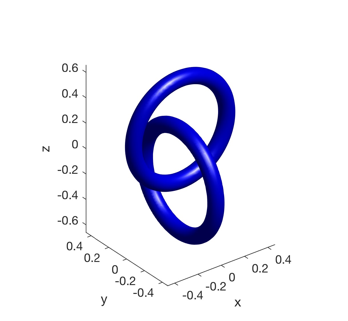
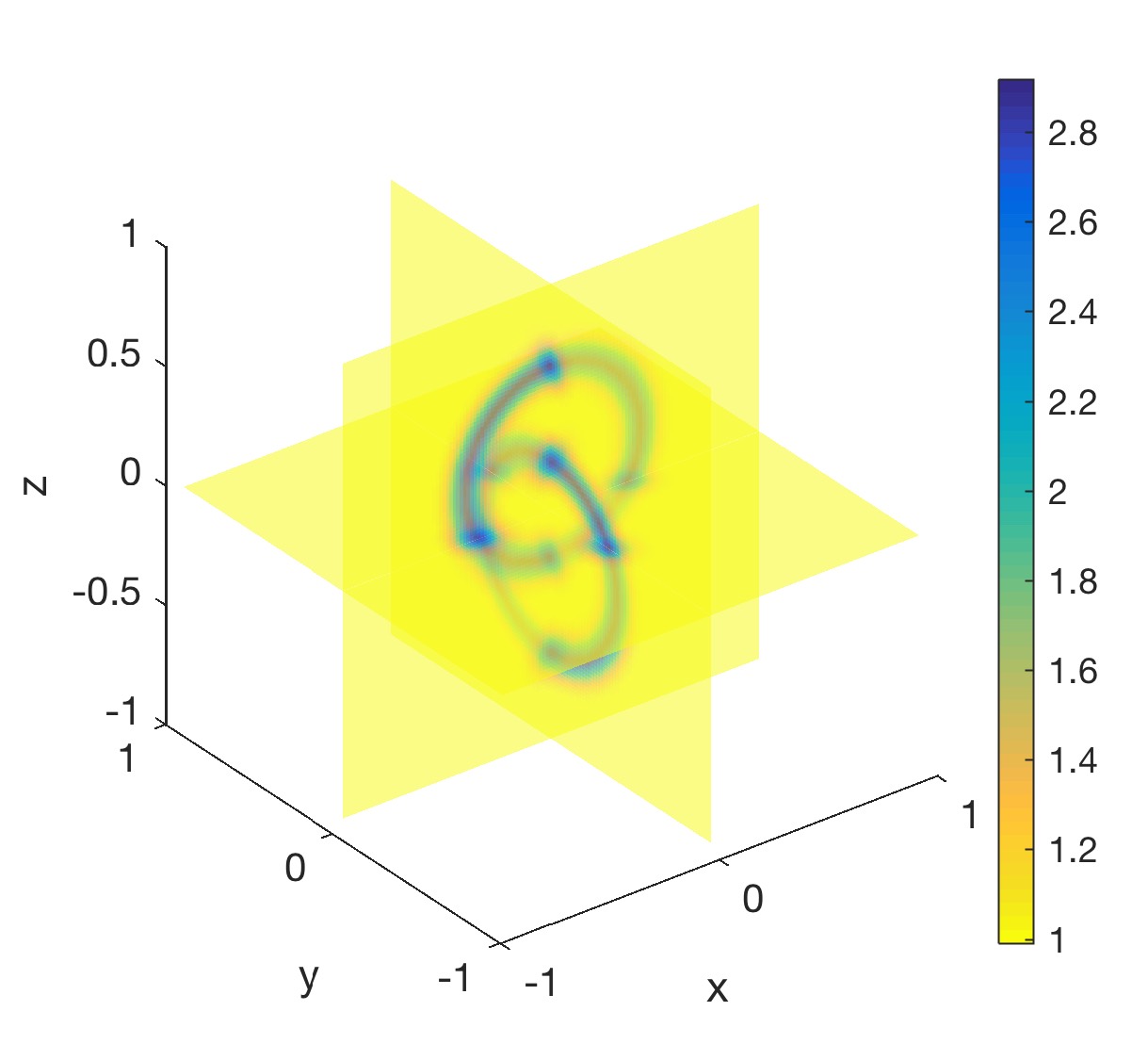
In this section, we define the conductivities γ1,γ2subscript𝛾1subscript𝛾2\gamma_{1},\gamma_{2} and γ3subscript𝛾3\gamma_{3} to be used for numerical experiments below. They will be the identity Id𝐼𝑑Id plus a tensor whose level set will be two interlocked tori like those shown on the right plot in Fig.1. Our experiments we will be conducted in the cubic domain, X=(1,1)3𝑋superscript113X=(-1,1)^{3}.

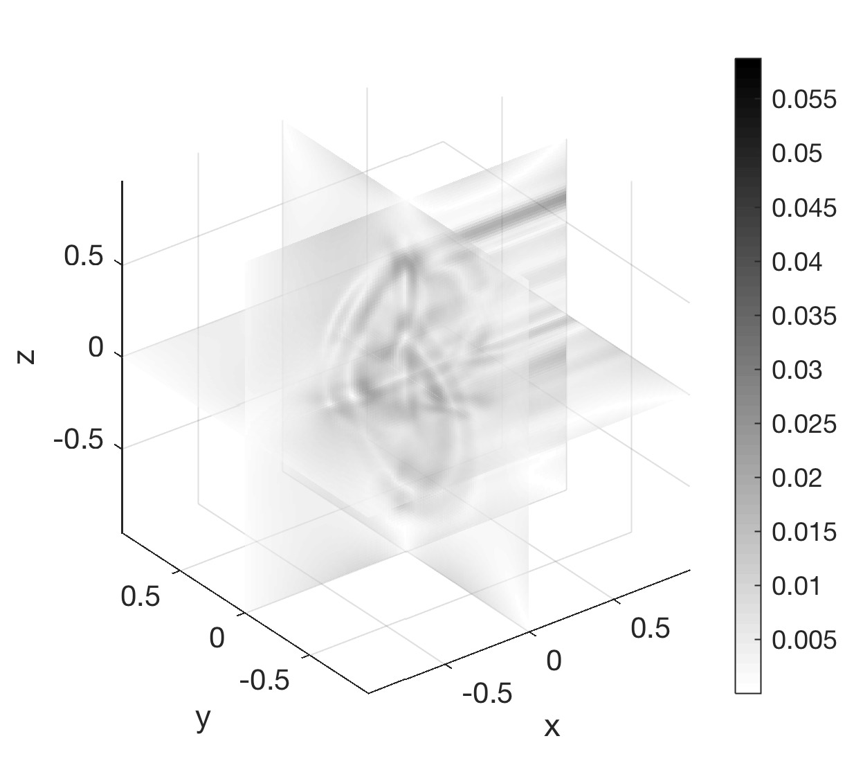
Refer to caption Refer to caption Refer to caption
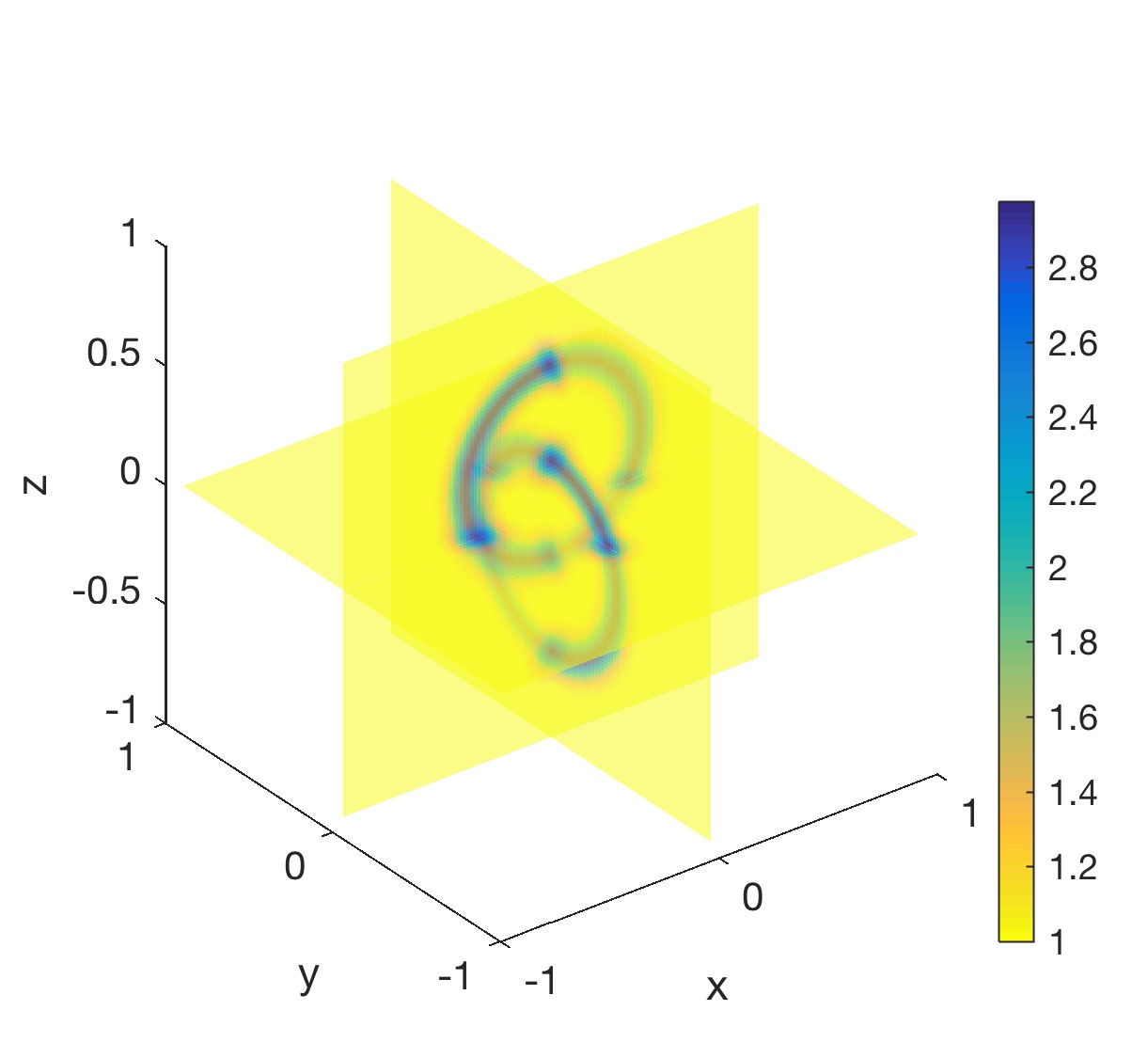
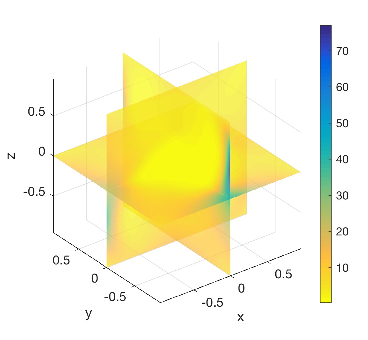
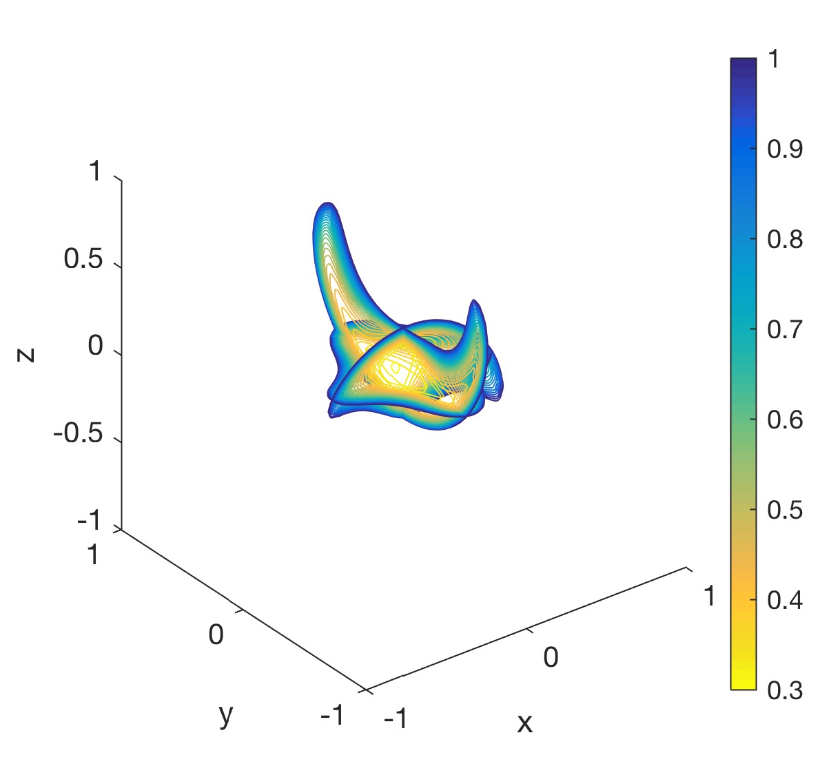
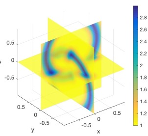
Figure 1: Parametrization of a torus (left), 3D slice plot of scalar interlocked tori γ1subscript𝛾1\gamma_{1} (64) (middle), and its isosurface {x:γ1(x)=1.8}conditional-setxsubscript𝛾1x1.8\{{\mathrm{x}}:\gamma_{1}({\mathrm{x}})=1.8\} (right)

Let us describe a torus T𝑇T by the quadruple T=(c,ϕ,R,r)𝑇citalic-ϕ𝑅𝑟T=({\mathrm{c}},\phi,R,r), see Fig.1 (left). The torus will be centered at c3csuperscript3{\mathrm{c}}\in\mathbb{R}^{3}, oriented by a unit vector ϕ3italic-ϕsuperscript3\phi\in\mathbb{R}^{3} orthogonal to the plane containing the generating circle, and have a radii of r𝑟r and R𝑅R for the small and great circles, respectively. Given a torus T𝑇T, let χTsubscript𝜒𝑇\chi_{T} be a smooth Gaussian kernel as a function of the distance to the generating circle. That is, χTsubscript𝜒𝑇\chi_{T} will have intensity one on the circle and will decay exponentially with respect to the distance to that circle.

χT(x):=exp(|xP(x)|22r2),assignsubscript𝜒𝑇xsuperscriptx𝑃x22superscript𝑟2\chi_{T}({\mathrm{x}}):=\exp\left(-\frac{|{\mathrm{x}}-P({\mathrm{x}})|^{2}}{2r^{2}}\right), (62)

where P(x)𝑃xP({\mathrm{x}}) maps xx{\mathrm{x}} to the its closest point on the generating circle of T𝑇T,

P(x):=c+Rxcxc,ϕϕ|xcxc,ϕϕ|.assign𝑃xc𝑅xcxcitalic-ϕitalic-ϕxcxcitalic-ϕitalic-ϕP({\mathrm{x}}):={\mathrm{c}}+R\,\frac{{\mathrm{x}}-{\mathrm{c}}-\left\langle{\mathrm{x}}-{\mathrm{c}},\phi\right\rangle\phi}{|{\mathrm{x}}-{\mathrm{c}}-\left\langle{\mathrm{x}}-{\mathrm{c}},\phi\right\rangle\phi|}. (63)

Then we define γTsubscript𝛾𝑇\gamma_{T} to be a smooth symmetric tensor of rank one, whose range belongs in the tangents of the generating circle of T𝑇T, whose amplitude will be adjusted by χTsubscript𝜒𝑇\chi_{T},

γT(x)subscript𝛾𝑇x\displaystyle\gamma_{T}({\mathrm{x}}) :=χT(x)(xc^×ϕ)(x^c×ϕ),wherex^c:=xc|xc|.formulae-sequenceassignabsenttensor-productsubscript𝜒𝑇x^subscriptxcitalic-ϕsubscript^xcitalic-ϕwhereassignsubscript^xcxcxc\displaystyle:=\chi_{T}({\mathrm{x}})(\widehat{{\mathrm{x}}_{\mathrm{c}}}\times\phi)\otimes(\widehat{{\mathrm{x}}}_{\mathrm{c}}\times\phi),\quad\text{where}\quad\widehat{{\mathrm{x}}}_{\mathrm{c}}:=\frac{{\mathrm{x}}-{\mathrm{c}}}{|{\mathrm{x}}-{\mathrm{c}}|}.

For each of our experiments, we will use two interlocked tori, one centered in the upper-half cube {z>0}𝑧0\{z>0\} (denoted by Tusubscript𝑇𝑢T_{u}), another centered in the lower-half cube {z<0}𝑧0\{z<0\} (denoted by Tdsubscript𝑇𝑑T_{d}). But we will vary the precise centers and radii.

Let the tori Tu1subscript𝑇𝑢1T_{u1}, Td1subscript𝑇𝑑1T_{d1}, Tu2subscript𝑇𝑢2T_{u2} and Td2subscript𝑇𝑑2T_{d2} given by

Tu1subscript𝑇𝑢1\displaystyle T_{u1} =(c1,ϕ1,R1,r1) and Td1=(c1,ϕ2,R1,r1) where {c1=(0,0,0.2),ϕ1=(1,0,0),ϕ2=(0,1,0),R1=0.4,r1=0.1,\displaystyle=({\mathrm{c}}_{1},\phi_{1},R_{1},r_{1})\quad\text{ and }\quad T_{d1}=(-{\mathrm{c}}_{1},\phi_{2},R_{1},r_{1})\quad\text{ where }\quad\left\{\begin{aligned} {\mathrm{c}}_{1}&=(0,0,0.2),\\ \phi_{1}&=(1,0,0),\\ \phi_{2}&=(0,1,0),\\ R_{1}&=0.4,\\ r_{1}&=0.1,\\ \end{aligned}\right.
Tu2subscript𝑇𝑢2\displaystyle T_{u2} =(c2,ϕ1,R2,r2) and Td2=(c2,ϕ2,R2,r2) where {c2=(0,0,0.5),R2=0.8,r2=0.1,\displaystyle=({\mathrm{c}}_{2},\phi_{1},R_{2},r_{2})\quad\text{ and }\quad T_{d2}=(-{\mathrm{c}}_{2},\phi_{2},R_{2},r_{2})\quad\text{ where }\quad\left\{\begin{aligned} {\mathrm{c}}_{2}&=(0,0,0.5),\\ R_{2}&=0.8,\\ r_{2}&=0.1,\\ \end{aligned}\right.

We then define the conductivities γ1,γ2subscript𝛾1subscript𝛾2\gamma_{1},\gamma_{2} and γ3subscript𝛾3\gamma_{3} as follows,

γ1subscript𝛾1\displaystyle\gamma_{1} =1+k1χTu1+k1χTd1 with k1=2,formulae-sequenceabsent1subscript𝑘1subscript𝜒subscript𝑇𝑢1subscript𝑘1subscript𝜒subscript𝑇𝑑1 with subscript𝑘12\displaystyle=1+k_{1}\chi_{T_{u1}}+k_{1}\chi_{T_{d1}}\qquad\text{ with }k_{1}=2, (64)
γ2subscript𝛾2\displaystyle\gamma_{2} =Id+k2γTu2+k2γTd2 with k2=2,formulae-sequenceabsent𝐼𝑑subscript𝑘2subscript𝛾subscript𝑇𝑢2subscript𝑘2subscript𝛾subscript𝑇𝑑2 with subscript𝑘22\displaystyle=Id+k_{2}\gamma_{T_{u2}}+k_{2}\gamma_{T_{d2}}\qquad\text{ with }k_{2}=2, (65)
γ3subscript𝛾3\displaystyle\gamma_{3} =Id+k3γTu2+k3γTd2 with k3=20.formulae-sequenceabsent𝐼𝑑subscript𝑘3subscript𝛾subscript𝑇𝑢2subscript𝑘3subscript𝛾subscript𝑇𝑑2 with subscript𝑘320\displaystyle=Id+k_{3}\gamma_{T_{u2}}+k_{3}\gamma_{T_{d2}}\qquad\text{ with }k_{3}=20. (66)

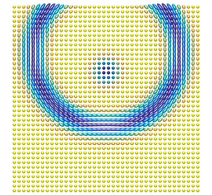
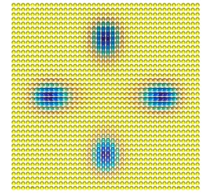
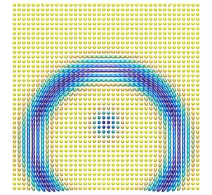
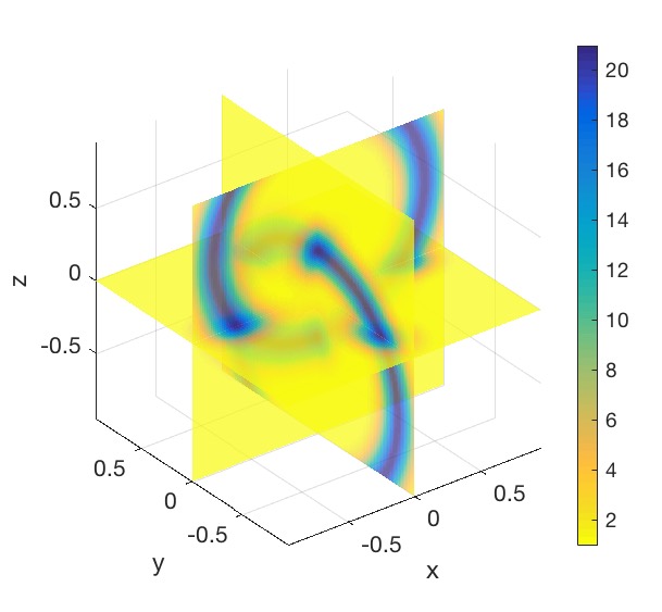
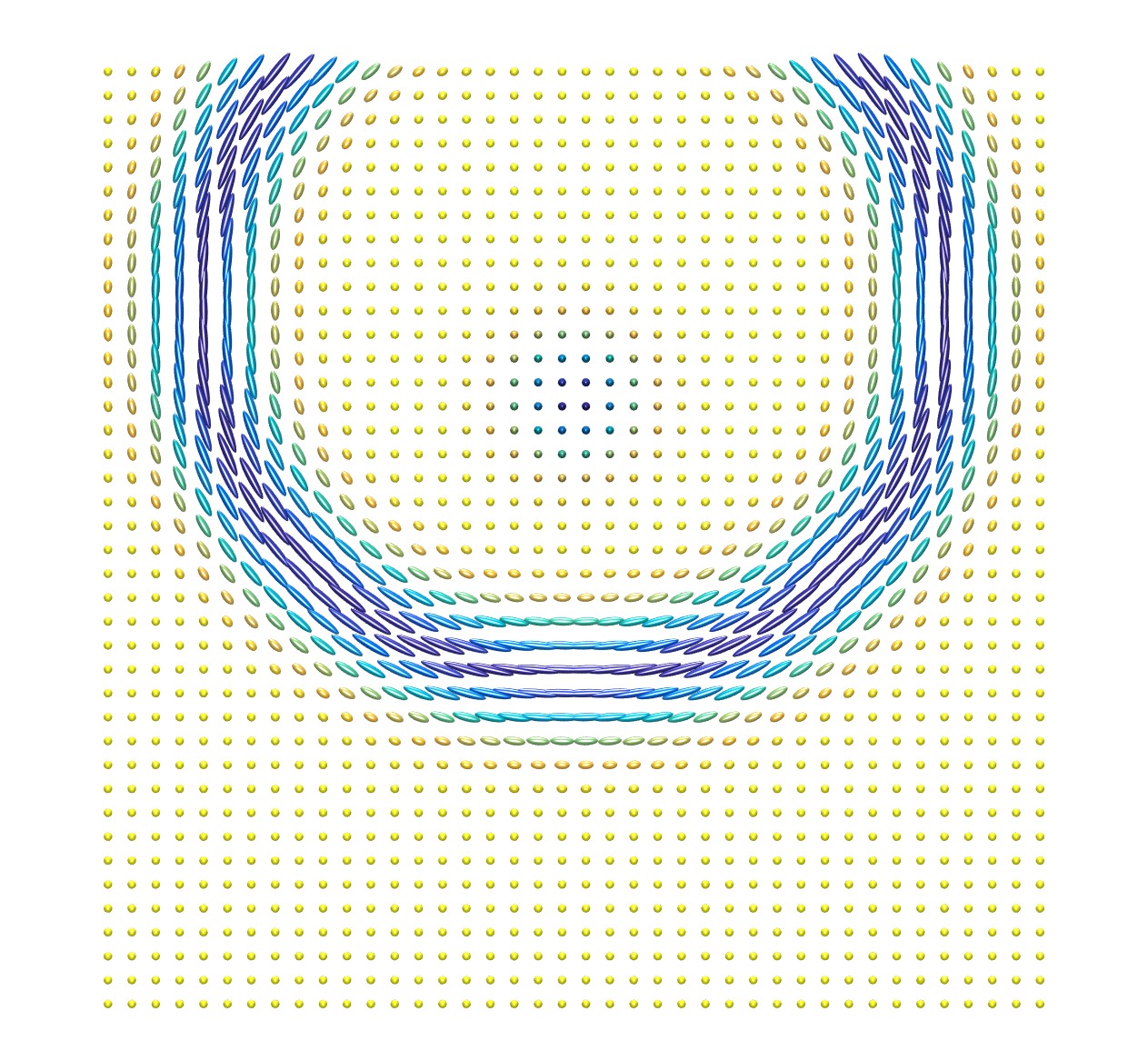
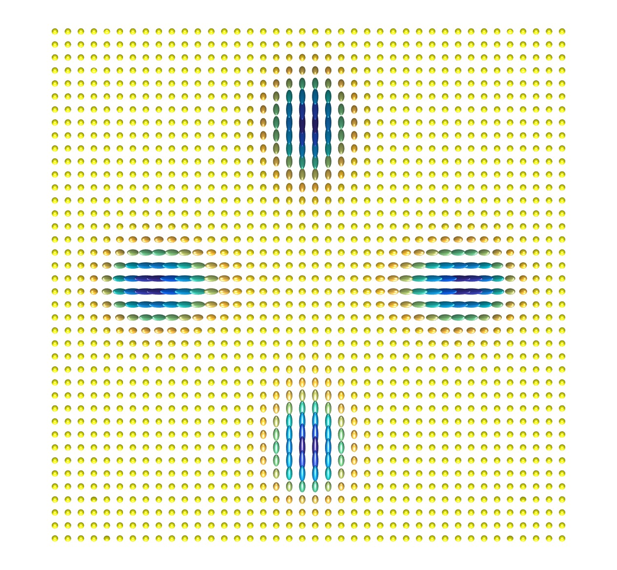
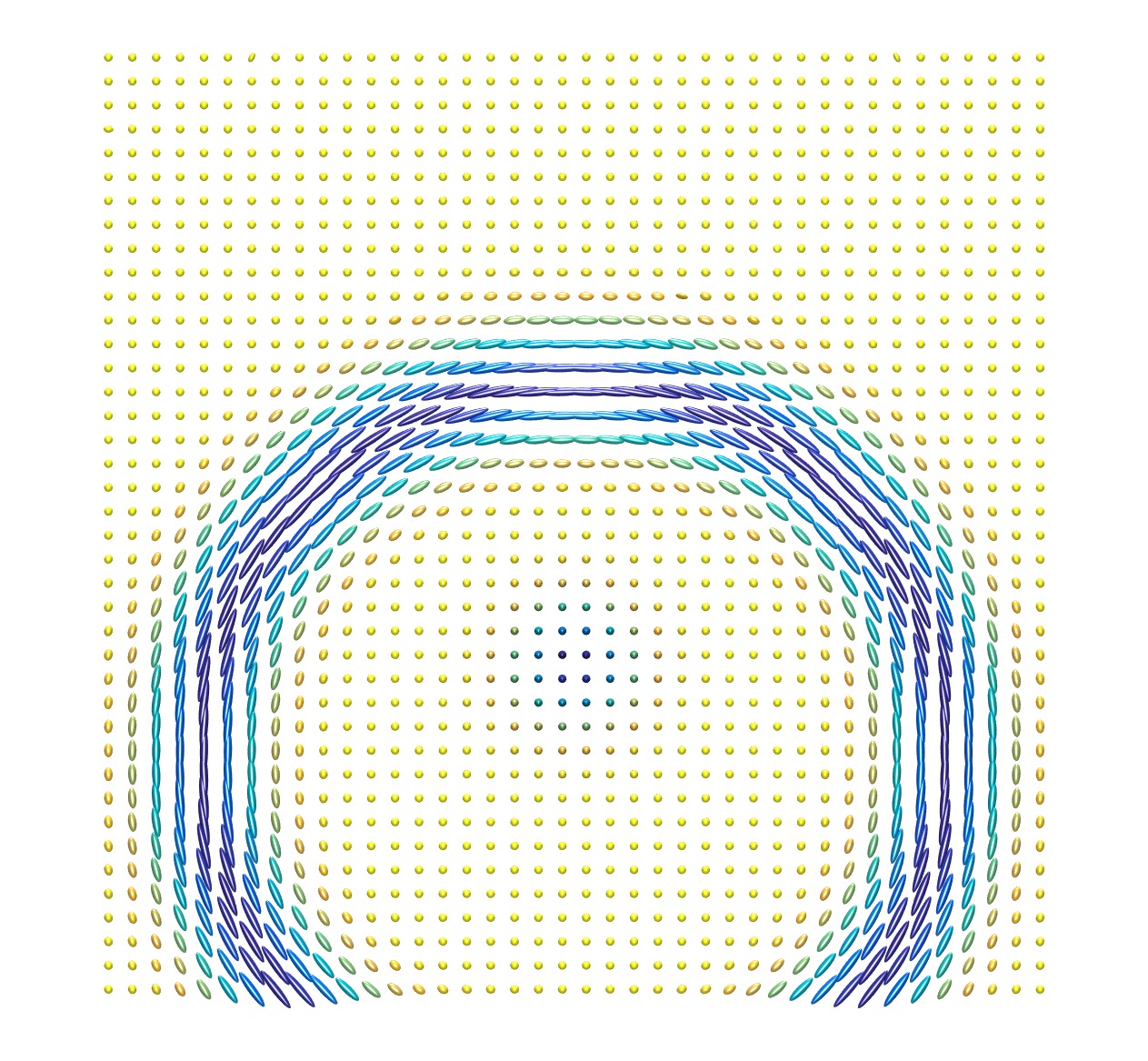
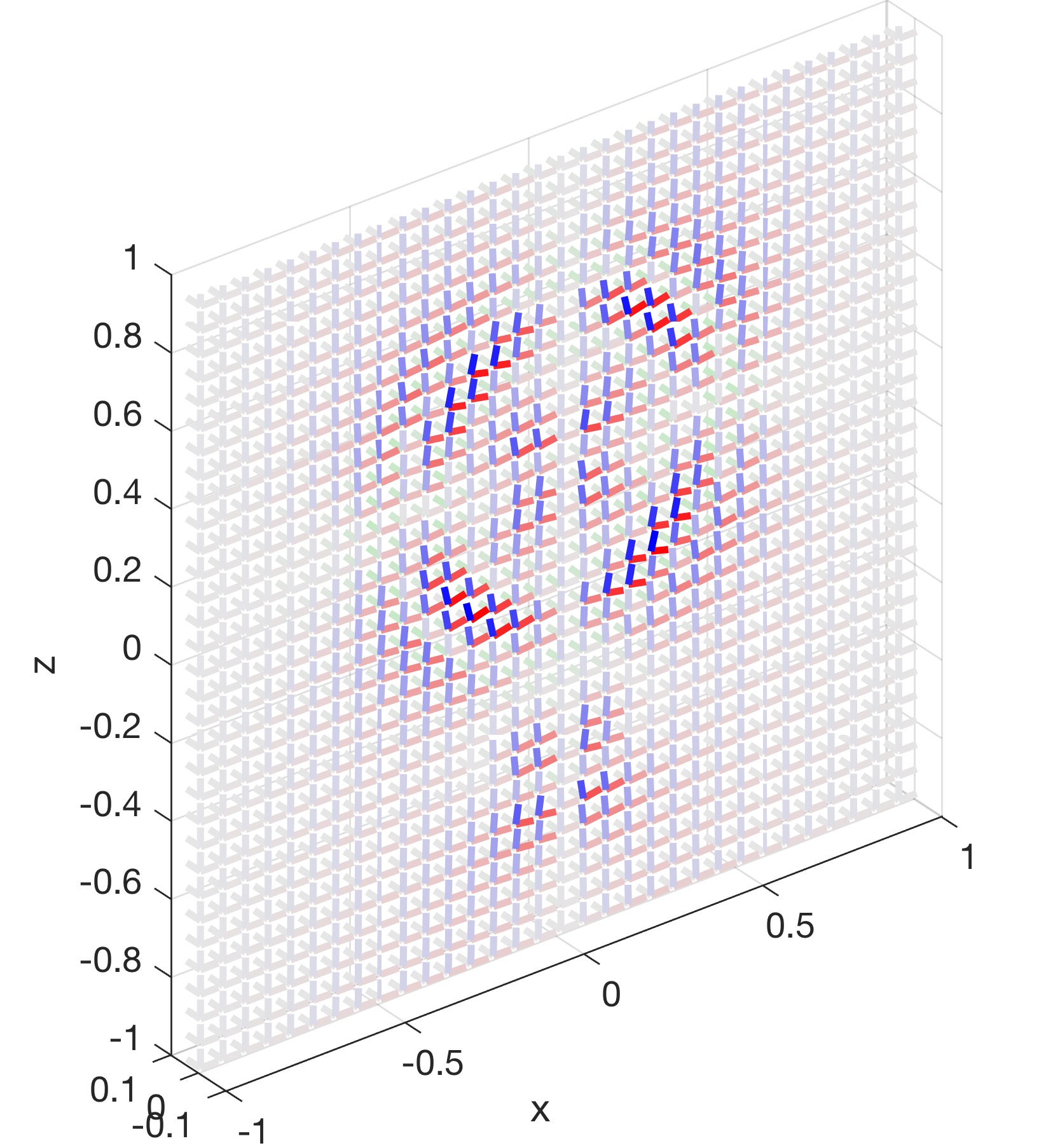
Note that γ1subscript𝛾1\gamma_{1} is a scalar corresponding to an isotropic case, whereas γ2subscript𝛾2\gamma_{2} and γ3subscript𝛾3\gamma_{3} are anisotropic. We plot the 3D slice plot of the scalar tori γ1subscript𝛾1\gamma_{1} along with an isosurface in Fig.1. The 3D slice plot of detγ𝛾\det\gamma as well as the representation of the anisotropy for each of the slices for γ1subscript𝛾1\gamma_{1} and γ2subscript𝛾2\gamma_{2} are given on Fig.2 and Fig.3, respectively. For this representation, we use the code developed in [16], where 3D ellipsoids are used to represent symmetric positive definite matrices; the principal axes correspond to the eigenvectors, and the widths along them correspond to the eigenvalues.
Refer to caption Refer to caption Refer to caption Refer to caption
3D slice plot of detγ2subscript𝛾2\det\gamma_{2} γ2subscript𝛾2\gamma_{2} on the yz𝑦𝑧yz-plane γ2subscript𝛾2\gamma_{2} on the xy𝑥𝑦xy-plane γ2subscript𝛾2\gamma_{2} on the xz𝑥𝑧xz-plane
Figure 2: Anisotropic interlocked tori γ2subscript𝛾2\gamma_{2} (65) of amplitude k2=2subscript𝑘22k_{2}=2. The axes of the ellipsoids represent the anisotropy at each spatial point [16].
Refer to caption Refer to caption Refer to caption Refer to caption
3D slice plot of detγ3subscript𝛾3\det\gamma_{3} γ3subscript𝛾3\gamma_{3} on the yz𝑦𝑧yz-plane γ3subscript𝛾3\gamma_{3} on the xy𝑥𝑦xy-plane γ3subscript𝛾3\gamma_{3} on the xz𝑥𝑧xz-plane
Figure 3: Anisotropic interlocked tori γ3subscript𝛾3\gamma_{3} (66) of amplitude k3=20subscript𝑘320k_{3}=20. The axes of the ellipsoids represent the anisotropy at each spatial point [16].

Our choice of conductivities is justified as follows. As is now well-known, certain conductivities γ𝛾\gamma are such that γ𝛾\gamma-harmonic extensions of global diffeomorphism of the boundary fail to make global diffeomorphism of the interior of the domain for dimension three (unlike in two). A famous example appears in [19], presented in the context of periodic structures. This was elaborated upon for a domain with boundary in [6]. The main idea therein is that for scalar interlocked tori with high conductivity (e.g., γ=1+kχT1+kχT2𝛾1𝑘subscript𝜒subscript𝑇1𝑘subscript𝜒subscript𝑇2\gamma=1+k\chi_{T_{1}}+k\chi_{T_{2}} with k𝑘k large), conduction of values along highly conductive regions creates topological changes in the isosurfaces of the solutions, which result in regions where three given solutions have linearly dependent gradients.

For our purposes in demonstrating the efficiency of our approach, we exacerbate these topological changes even more, by using the anisotropic tensor γ3subscript𝛾3\gamma_{3} defined in (66) whose diffusion is especially high along the generating circles of the two tori.

5.2 Numerical implementation

The forward problem for the three experiments that appear in Sections 5.3, 5.4, and 5.5 are solved using the finite element method [18]: the solutions to the conductivity problems are computed using piecewise quadratic elements on an unstructured tetrahedral mesh with maximal diameter hmax=0.05subscriptmax0.05h_{\textrm{max}}=0.05. The power densities {Hij}subscript𝐻𝑖𝑗\{H_{ij}\} are computed by first evaluating the finite element solutions and their gradients for uniform Cartesian grid-points, then computing the inner-product point-wise. The uniform grid of size 128×128×128128128128128\times 128\times 128 was used.

Once the power densities are generated as above, various reconstruction procedures outlined in Sections 3 and 4, are performed solely on the uniform Cartesian grid. For exampe, these procedures include the computation of the dynamical system (8) for quaternions, and the solution of the Poisson problems that follow from (34), (57), and (61) are solved on the uniform grid using the finite difference method [28]. Gradient computations necessary for preparing these systems are also computed using second-order finite differences.

5.3 Isotropic reconstructions via dynamical system

Experiment 1.

Here we reconstruct the scalar interlocked tori γ1subscript𝛾1\gamma_{1} (64) from the power densities Hij(x)subscript𝐻𝑖𝑗xH_{ij}({\mathrm{x}}) (i,j=1,2,3formulae-sequence𝑖𝑗123i,j=1,2,3) of three solutions

u1(x),u2(x),u3(x),subscript𝑢1xsubscript𝑢2xsubscript𝑢3xu_{1}({\mathrm{x}}),\qquad u_{2}({\mathrm{x}}),\qquad u_{3}({\mathrm{x}}), (67)

which satisfy the boundary conditions

u1(x)|X=x,u2(x)|X=y,u3(x)|X=z.u_{1}({\mathrm{x}})\big{\rvert}_{\partial X}=x,\qquad u_{2}({\mathrm{x}})\big{\rvert}_{\partial X}=y,\qquad u_{3}({\mathrm{x}})\big{\rvert}_{\partial X}=z. (68)

The determinant of the gradients of the solutions, i.e. det(u1,u2,u3)subscript𝑢1subscript𝑢2subscript𝑢3\det(\nabla u_{1},\nabla u_{2},\nabla u_{3}), does not vanish for this set of solutions, as shown in Fig.4.
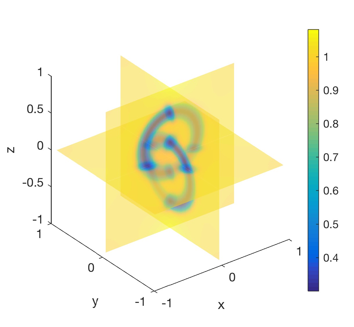
Refer to caption
Figure 4: Exp. 1: det(u1,u2,u3)subscript𝑢1subscript𝑢2subscript𝑢3\det(\nabla u_{1},\nabla u_{2},\nabla u_{3}) for three solutions (67, 68) obtained for the smooth scalar conductivity γ1subscript𝛾1\gamma_{1} (64). Computed minimum: 0.3000.

We proceed to use the algorithm proposed in Section 3 to reconstruct γ1subscript𝛾1\gamma_{1}. The dynamical system (8) for quaternions is solved along the straight line in the direction of the x𝑥x-axis, along a Cartesian grid. The computed quaternionic system allows the reconstruction of the SO(3)𝑆𝑂3SO(3)-valued function arising from the local gradient system (6). We denote this function by R=(R1,R2,R3)𝑅subscript𝑅1subscript𝑅2subscript𝑅3R=(R_{1},R_{2},R_{3}) where Risubscript𝑅𝑖R_{i} is the i𝑖i-th basis vector after applying the rotation matrix to the canonical basis. The true R𝑅R and the reconstruction error R𝑅R are visualized in and Fig.5, respectively. In the relative error, one can clearly see the direction-dependence of the reconstruction, as the errors accumulate as the dynamical system is being integrated from the boundary at x=1𝑥1x=-1.

Finally, we reconstruct γ1subscript𝛾1\gamma_{1} by solving the Poisson’s problem (34). The reconstruction, along with its corresponding relative error are plotted in Fig.6. The error is concentrated near the region of high conductivity at the generating circle of the two tori. The reconstruction errors are summarized in Table 1. The relative L1superscript𝐿1L^{1} error is at 0.1%percent0.10.1\% and pointwise relative error is less than 6%percent66\%.

γ1subscript𝛾1\gamma_{1}
Rel. L1superscript𝐿1L^{1} error 0.00127075
Rel. L2superscript𝐿2L^{2} error 0.00659273
Rel. Lsuperscript𝐿L^{\infty} error 0.05968462
Max. pointwise rel. error 0.06503202
Table 1: Exp. 1: Summary of reconstruction error for γ1subscript𝛾1\gamma_{1} (64).
Refer to caption Refer to caption
Figure 5: Exp. 1: True R𝑅R, visualized by showing three components of the rotated standard basis (𝐞1,𝐞2,𝐞3)subscript𝐞1subscript𝐞2subscript𝐞3(\mathbf{e}_{1},\mathbf{e}_{2},\mathbf{e}_{3}) under the action of R𝑅R, color-coded by red, green and blue, respectively (left). The strength of the colors indicate deviation from the identity measured in Frobenius norm. 3D slice plot of the relative reconstruction error, also measured in the Frobenius norm (right).
Refer to caption Refer to caption Refer to caption
Figure 6: Exp. 1: 3D slice plot of the reconstruction of smooth scalar interlocked tori γ1subscript𝛾1\gamma_{1} (64) (left) (to be compared with Fig.1, middle), the relative pointwise error (middle), and 1D comparison plot for γ1subscript𝛾1\gamma_{1} and its reconstruction, along the line parallel to the x𝑥x-axis through (y,z)=(0,0.25)𝑦𝑧00.25(y,z)=(0,0.25) (right). The line is indicated by the red dashed line in the middle plot.

5.4 Anisotropic reconstructions using 3+2323+2 solutions

Experiment 2.

We first demonstrate the success of the approach in a perturbative case where the unknown tensor γ2subscript𝛾2\gamma_{2} (65) is close enough to a known γ0subscript𝛾0\gamma_{0}, for which some background solutions (u1,u2,u3,v1,v2)subscript𝑢1subscript𝑢2subscript𝑢3subscript𝑣1subscript𝑣2(u_{1},u_{2},u_{3},v_{1},v_{2}) are known to fulfill the maximality conditions globally, that is, (u1,u2,u3)subscript𝑢1subscript𝑢2subscript𝑢3(\nabla u_{1},\nabla u_{2},\nabla u_{3}) forms a basis throughout X𝑋X. By continuity of solutions with respect to the conductivity, generating power densities using the traces of the background solutions will provide functionals which still satisfy the maximality conditions globally, so the proposed algorithm should recover γ2subscript𝛾2\gamma_{2} successfully.

Namely, let γ0=Idsubscript𝛾0𝐼𝑑\gamma_{0}=Id the identity tensor, and let the background conductivity solutions (u1,u2,u3,v1,v2)subscript𝑢1subscript𝑢2subscript𝑢3subscript𝑣1subscript𝑣2(u_{1},u_{2},u_{3},v_{1},v_{2}) be given by

u1=x,u2=y,u3=z,v1=(x+2)(y+2),v2=(x+2)(z+2).formulae-sequencesubscript𝑢1𝑥formulae-sequencesubscript𝑢2𝑦formulae-sequencesubscript𝑢3𝑧formulae-sequencesubscript𝑣1𝑥2𝑦2subscript𝑣2𝑥2𝑧2\displaystyle u_{1}=x,\quad u_{2}=y,\quad u_{3}=z,\quad v_{1}=(x+2)(y+2),\quad v_{2}=(x+2)(z+2).

For such solutions, we can compute directly that det(u1,u2,u3)=1subscript𝑢1subscript𝑢2subscript𝑢31\det(\nabla u_{1},\nabla u_{2},\nabla u_{3})=1 everywhere, and that the eight matrices defined in (56) are constant and equal to

𝐙1subscript𝐙1\displaystyle\mathbf{Z}_{1} =𝐞1𝐞2+𝐞2𝐞1,𝐙1HΩ1=𝐞1𝐞3,𝐙1HΩ2=𝐞2𝐞3,𝐙1HΩ3=𝐞2𝐞2𝐞1𝐞1,formulae-sequenceabsenttensor-productsubscript𝐞1subscript𝐞2tensor-productsubscript𝐞2subscript𝐞1formulae-sequencesubscript𝐙1𝐻subscriptΩ1tensor-productsubscript𝐞1subscript𝐞3formulae-sequencesubscript𝐙1𝐻subscriptΩ2tensor-productsubscript𝐞2subscript𝐞3subscript𝐙1𝐻subscriptΩ3tensor-productsubscript𝐞2subscript𝐞2tensor-productsubscript𝐞1subscript𝐞1\displaystyle=\mathbf{e}_{1}\otimes\mathbf{e}_{2}+\mathbf{e}_{2}\otimes\mathbf{e}_{1},\ \mathbf{Z}_{1}H\Omega_{1}=\mathbf{e}_{1}\otimes\mathbf{e}_{3},\ \mathbf{Z}_{1}H\Omega_{2}=-\mathbf{e}_{2}\otimes\mathbf{e}_{3},\ \mathbf{Z}_{1}H\Omega_{3}=\mathbf{e}_{2}\otimes\mathbf{e}_{2}-\mathbf{e}_{1}\otimes\mathbf{e}_{1},
𝐙2subscript𝐙2\displaystyle\mathbf{Z}_{2} =𝐞1𝐞3+𝐞3𝐞1,𝐙2HΩ1=𝐞1𝐞2,𝐙2HΩ2=𝐞1𝐞1𝐞3𝐞3,𝐙2HΩ3=𝐞3𝐞2.formulae-sequenceabsenttensor-productsubscript𝐞1subscript𝐞3tensor-productsubscript𝐞3subscript𝐞1formulae-sequencesubscript𝐙2𝐻subscriptΩ1tensor-productsubscript𝐞1subscript𝐞2formulae-sequencesubscript𝐙2𝐻subscriptΩ2tensor-productsubscript𝐞1subscript𝐞1tensor-productsubscript𝐞3subscript𝐞3subscript𝐙2𝐻subscriptΩ3tensor-productsubscript𝐞3subscript𝐞2\displaystyle=\mathbf{e}_{1}\otimes\mathbf{e}_{3}+\mathbf{e}_{3}\otimes\mathbf{e}_{1},\ \mathbf{Z}_{2}H\Omega_{1}=-\mathbf{e}_{1}\otimes\mathbf{e}_{2},\ \mathbf{Z}_{2}H\Omega_{2}=\mathbf{e}_{1}\otimes\mathbf{e}_{1}-\mathbf{e}_{3}\otimes\mathbf{e}_{3},\ \mathbf{Z}_{2}H\Omega_{3}=\mathbf{e}_{3}\otimes\mathbf{e}_{2}.

Therefore these matrices span {Id}M3()superscript𝐼𝑑perpendicular-tosubscript𝑀3\{Id\}^{\perp}\subset M_{3}(\mathbb{R}) at every point. Then by a perturbation argument, for γ2subscript𝛾2\gamma_{2} close enough to Id𝐼𝑑Id, the solutions of the problem (γ2u)=0subscript𝛾2𝑢0\nabla\cdot(\gamma_{2}\nabla u)=0 with u|Xevaluated-at𝑢𝑋u|_{\partial X} sucessively equal to the traces of (u1,u2,u3,v1,v2)subscript𝑢1subscript𝑢2subscript𝑢3subscript𝑣1subscript𝑣2(u_{1},u_{2},u_{3},v_{1},v_{2}), still satisfy the conditions of Hypothesis 4.2 globally, setting the stage for a sucessful reconstruction.
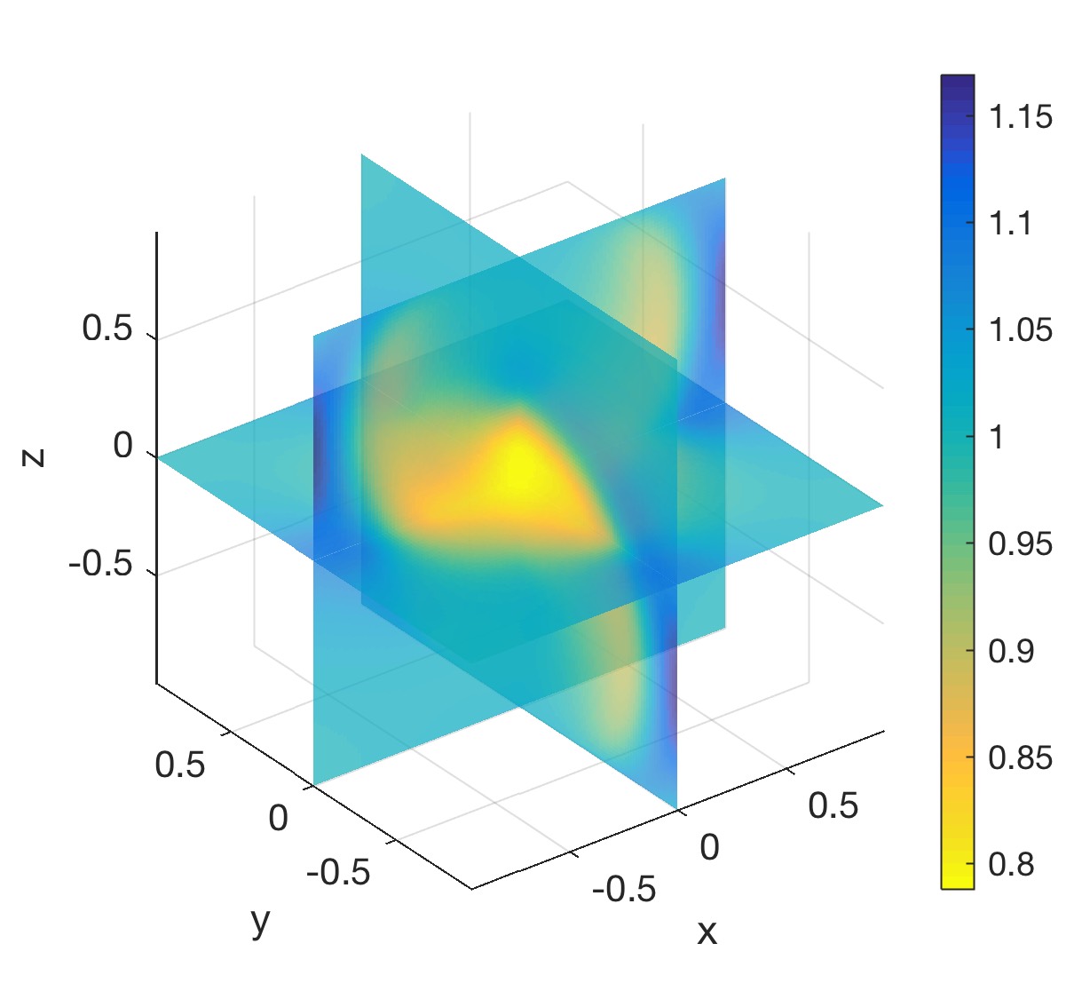
Refer to caption Refer to caption
Figure 7: Exp. 2: 3D slice plot of det(u1,u2,u3)subscript𝑢1subscript𝑢2subscript𝑢3\det(\nabla u_{1},\nabla u_{2},\nabla u_{3}) in which the computed minimum is 0.7881 (left). 3D slice plot of the error for reconstructed γ~2subscript~𝛾2\tilde{\gamma}_{2} in relative Frobenius norm (right).

First, we check numerically that the determinant of the gradients det(u1,u2,u3)subscript𝑢1subscript𝑢2subscript𝑢3\det(\nabla u_{1},\nabla u_{2},\nabla u_{3}) do not vanish. We plot the determinant to the left in Fig.7, which reveals that the determinant stays away from zero. Then we reconstruct the anisotropic tensor γ~2subscript~𝛾2\tilde{\gamma}_{2} using the 3+2 algorithm outlined in Section 4.2. The reconstruction error is shown in Fig.7 (right).

Using the reconstructed γ~2subscript~𝛾2\tilde{\gamma}_{2} we solve the Poisson problem (57), to obtain the scaling τ2subscript𝜏2\tau_{2}. The reconstructed τ2subscript𝜏2\tau_{2} and its relative error is shown in Fig.8. Finally, the error for the reconstructed γ2subscript𝛾2\gamma_{2} itself is shown to the right in the same figure. The reconstruction errors are summarized in Table 2. The relative L1superscript𝐿1L^{1} error is at 0.4%percent0.40.4\% and pointwise relative error is less than 15%percent1515\%. The volume of the domain that incurs pointwise relative error larger than 10%percent1010\% is 0.005%percent0.0050.005\%, hence the error is highly localized.

The error for the anisotropic part mostly originates from the approximation of the matrices orthogonal to (56) and (58), see discussion at the end of Experiment 3 (Section 5.5).

γ~2subscript~𝛾2\tilde{\gamma}_{2} τ2subscript𝜏2\tau_{2} γ2subscript𝛾2\gamma_{2}
Rel. L1superscript𝐿1L^{1} error 0.00375946 0.00030364 0.00407776
Rel. L2superscript𝐿2L^{2} error 0.00789942 0.00091769 0.00909787
Rel. Lsuperscript𝐿L^{\infty} error 0.11603989 0.01264201 0.12900887
Max. pointwise rel. error 0.16959084 0.01248439 0.15545096
Table 2: Exp. 2: Summary of reconstruction error for γ2subscript𝛾2\gamma_{2} (65). The error for the tensor-valued functions computed pointwise by the Frobenius norm.
Refer to caption Refer to caption Refer to caption
Figure 8: Exp. 2: 3D slice plots of reconstruction of τ2subscript𝜏2\tau_{2} (left), relative error for τ2subscript𝜏2\tau_{2} (middle) and relative error for γ2subscript𝛾2\gamma_{2} in log-scale (right). The errors are in terms of the Frobenius norm.

5.5 Anisotropic reconstructions using more than 3+2323+2 solutions

Experiment 3.

Here we perform the experiment for γ3subscript𝛾3\gamma_{3} (66) for which the 3+2 reconstruction algorithm fails, due to the fact that the gradient of three solutions become linearly dependent in some parts of the domain. To overcome this difficulty, we will employ additional solutions and employ the stabilized algorithm proposed in Section 4.3. We will use the solution set (u1,u2,u3,u4,u5,u6,v1,v2,v3)subscript𝑢1subscript𝑢2subscript𝑢3subscript𝑢4subscript𝑢5subscript𝑢6subscript𝑣1subscript𝑣2subscript𝑣3(u_{1},u_{2},u_{3},u_{4},u_{5},u_{6},v_{1},v_{2},v_{3}) which satisfy the Dirichlet data

u1|X\displaystyle u_{1}\big{\rvert}_{\partial X} =x,u4|X=x+32(z+2)2,v1|X=(x+2)(y+2),\displaystyle=x,\qquad u_{4}\big{\rvert}_{\partial X}=x+\frac{3}{2}(z+2)^{2},\qquad v_{1}\big{\rvert}_{\partial X}=(x+2)(y+2),
u2|X\displaystyle u_{2}\big{\rvert}_{\partial X} =y,u5|X=y+32(x+2)2,v2|X=(y+2)(z+2),\displaystyle=y,\qquad u_{5}\big{\rvert}_{\partial X}=y+\frac{3}{2}(x+2)^{2},\qquad v_{2}\big{\rvert}_{\partial X}=(y+2)(z+2),
u3|X\displaystyle u_{3}\big{\rvert}_{\partial X} =z,u6|X=z+32(y+2)2,v3|X=(z+2)(x+2).\displaystyle=z,\qquad u_{6}\big{\rvert}_{\partial X}=z+\frac{3}{2}(y+2)^{2},\qquad v_{3}\big{\rvert}_{\partial X}=(z+2)(x+2).

We will define the triples of these solutions as follows,
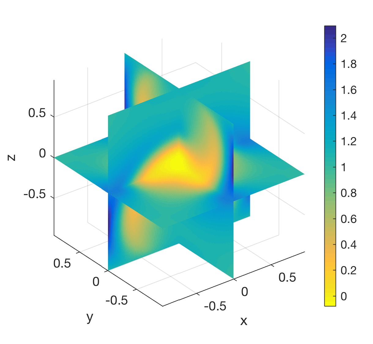
U(1):=(u1,u2,u3),U(2):=(u4,u2,u3),U(3):=(u1,u5,u3),U(4):=(u1,u2,u6).formulae-sequenceassignsuperscript𝑈1subscript𝑢1subscript𝑢2subscript𝑢3formulae-sequenceassignsuperscript𝑈2subscript𝑢4subscript𝑢2subscript𝑢3formulae-sequenceassignsuperscript𝑈3subscript𝑢1subscript𝑢5subscript𝑢3assignsuperscript𝑈4subscript𝑢1subscript𝑢2subscript𝑢6U^{(1)}:=(u_{1},u_{2},u_{3}),\quad U^{(2)}:=(u_{4},u_{2},u_{3}),\quad U^{(3)}:=(u_{1},u_{5},u_{3}),\quad U^{(4)}:=(u_{1},u_{2},u_{6}).
Refer to caption Refer to caption Refer to caption Refer to caption
detDU(1)𝐷superscript𝑈1\det DU^{(1)} detDU(2)𝐷superscript𝑈2\det DU^{(2)} detDU(3)𝐷superscript𝑈3\det DU^{(3)} detDU(4)𝐷superscript𝑈4\det DU^{(4)}
Figure 9: Exp. 3: Determinants detDU(j)𝐷superscript𝑈𝑗\det DU^{(j)} for j=1,2,3,4𝑗1234j=1,2,3,4. Top row: slice plots. Bottom row: iso-lines corresponding to the negative values.

The determinant for each of these triples are then denoted

detDU(1)=det(u1,u2,u3),𝐷superscript𝑈1subscript𝑢1subscript𝑢2subscript𝑢3\displaystyle\det DU^{(1)}=\det(\nabla u_{1},\nabla u_{2},\nabla u_{3}), detDU(2)=det(u4,u2,u3),𝐷superscript𝑈2subscript𝑢4subscript𝑢2subscript𝑢3\displaystyle\qquad\det DU^{(2)}=\det(\nabla u_{4},\nabla u_{2},\nabla u_{3}),
detDU(3)=det(u1,u5,u3),𝐷superscript𝑈3subscript𝑢1subscript𝑢5subscript𝑢3\displaystyle\det DU^{(3)}=\det(\nabla u_{1},\nabla u_{5},\nabla u_{3}), detDU(4)=det(u1,u2,u6).𝐷superscript𝑈4subscript𝑢1subscript𝑢2subscript𝑢6\displaystyle\qquad\det DU^{(4)}=\det(\nabla u_{1},\nabla u_{2},\nabla u_{6}).

For each of these triples, the determinant detDU(j)𝐷superscript𝑈𝑗\det DU^{(j)} vanishes and switches sign inside X𝑋X, as shown in the slice plots on Fig.9. Therefore, the determinants of H(j)superscript𝐻𝑗H^{(j)} (j=1,2,3,4𝑗1234j=1,2,3,4) also vanish and the 3+2 algorithm (based on a single triple of solutions) from Section 4.2 fails. On the other hand, one may visualize on Fig.10 that the quantity

|detDU(1)|2+|detDU(2)|2+|detDU(3)|2+|detDU(4)|2superscript𝐷superscript𝑈12superscript𝐷superscript𝑈22superscript𝐷superscript𝑈32superscript𝐷superscript𝑈42|\det DU^{(1)}|^{2}+|\det DU^{(2)}|^{2}+|\det DU^{(3)}|^{2}+|\det DU^{(4)}|^{2}

is everywhere positive on X𝑋X (that is, the intersection of the zero sets corresponding to the four triples is empty), setting the stage for an implementation of the stabilized algorithm.

Now one may reconstruct γ~(j)superscript~𝛾𝑗\tilde{\gamma}^{(j)} as in the 3+2 algorithm, for each solution triples U(j)superscript𝑈𝑗U^{(j)} but such individual reconstructions fail locally, though never simultaneously. The choices of solutions to use for the individual 3+2 algorithms are,

U(1)superscript𝑈1\displaystyle U^{(1)} =(u1,u2,u3) with (v1,v2),absentsubscript𝑢1subscript𝑢2subscript𝑢3 with subscript𝑣1subscript𝑣2\displaystyle=(u_{1},u_{2},u_{3})\quad\text{ with }\quad(v_{1},v_{2}),
U(2)superscript𝑈2\displaystyle U^{(2)} =(u4,u2,u3) with (v2,v3),absentsubscript𝑢4subscript𝑢2subscript𝑢3 with subscript𝑣2subscript𝑣3\displaystyle=(u_{4},u_{2},u_{3})\quad\text{ with }\quad(v_{2},v_{3}),
U(3)superscript𝑈3\displaystyle U^{(3)} =(u1,u5,u3) with (v1,v2),absentsubscript𝑢1subscript𝑢5subscript𝑢3 with subscript𝑣1subscript𝑣2\displaystyle=(u_{1},u_{5},u_{3})\quad\text{ with }\quad(v_{1},v_{2}),
U(4)superscript𝑈4\displaystyle U^{(4)} =(u1,u2,u6) with (v2,v3).absentsubscript𝑢1subscript𝑢2subscript𝑢6 with subscript𝑣2subscript𝑣3\displaystyle=(u_{1},u_{2},u_{6})\quad\text{ with }\quad(v_{2},v_{3}).

The individual errors are shown in Fig.11. However, when they are combined in the system (61) one can successfully recover the scaling τ3subscript𝜏3\tau_{3}, as shown in Fig.13.

For reconstruction of γ~3subscript~𝛾3\tilde{\gamma}_{3}, one may weight each individual reconstructions γ~(j)superscript~𝛾𝑗\tilde{\gamma}^{(j)} by |H(j)|superscript𝐻𝑗|H^{(j)}|,

γ~3,H:=|H(1)|γ~(1)+|H(2)|γ~(2)+|H(3)|γ~(3)+|H(4)|γ~(4)det(|H(1)|γ~(1)+|H(2)|γ~(2)+|H(3)|γ~(3)+|H(4)|γ~(4))1/3.assignsubscript~𝛾3Hsuperscript𝐻1superscript~𝛾1superscript𝐻2superscript~𝛾2superscript𝐻3superscript~𝛾3superscript𝐻4superscript~𝛾4superscriptsuperscript𝐻1superscript~𝛾1superscript𝐻2superscript~𝛾2superscript𝐻3superscript~𝛾3superscript𝐻4superscript~𝛾413\tilde{\gamma}_{3,\mathrm{H}}:=\frac{|H^{(1)}|\tilde{\gamma}^{(1)}+|H^{(2)}|\tilde{\gamma}^{(2)}+|H^{(3)}|\tilde{\gamma}^{(3)}+|H^{(4)}|\tilde{\gamma}^{(4)}}{\det\left(|H^{(1)}|\tilde{\gamma}^{(1)}+|H^{(2)}|\tilde{\gamma}^{(2)}+|H^{(3)}|\tilde{\gamma}^{(3)}+|H^{(4)}|\tilde{\gamma}^{(4)}\right)^{1/3}}. (69)

On the other hand, we observe numerically that the errors for the individual γ~(j)superscript~𝛾𝑗\tilde{\gamma}^{(j)}’s are inversely proportional to γ~(j)Fsubscriptdelimited-∥∥superscript~𝛾𝑗𝐹\lVert\tilde{\gamma}^{(j)}\rVert_{F}. An intuitive argument for this is that the orthogonalization to compute Bsuperscript𝐵B^{\prime} (see Step A in Section 4.2 or its stabilized equivalent Step A’ in Section 4.3) corresponds more naturally to the Frobenius norm. Hence Bsuperscript𝐵B^{\prime} is most accurate when normalized in this norm, and hence whenever the reconstructed approximation to γ~(j)superscript~𝛾𝑗\tilde{\gamma}^{(j)} has a large Frobenius norm γ~(j)Fsubscriptdelimited-∥∥superscript~𝛾𝑗𝐹\lVert\tilde{\gamma}^{(j)}\rVert_{F}, one may expect a large error. To exploit this observation, we first choose to exclude the approximation among {γ~(j)}superscript~𝛾𝑗\{\tilde{\gamma}^{(j)}\} that has the largest Frobenius norm. To this end, we first define the spatially dependent index set

𝒥(x)={1,2,3,4}argmaxi{γ~(i)(x)F}.𝒥x1234subscriptargmax𝑖subscriptdelimited-∥∥superscript~𝛾𝑖x𝐹\mathcal{J}({\mathrm{x}})=\{1,2,3,4\}\setminus\textrm{argmax}_{i}\{\lVert\tilde{\gamma}^{(i)}({\mathrm{x}})\rVert_{F}\}. (70)

Then, we define the approximation γ~3,Fsubscript~𝛾3F\tilde{\gamma}_{3,\mathrm{F}} using the weighted sum of the remaining members of {γ~(j)}superscript~𝛾𝑗\{\tilde{\gamma}^{(j)}\},

γ~3,F(x):=j𝒥(x)γ~(j)γ~(j)F/det(j𝒥(x)γ~(j)γ~(j)F)1/3.assignsubscript~𝛾3Fxsubscript𝑗𝒥x/superscript~𝛾𝑗subscriptdelimited-∥∥superscript~𝛾𝑗𝐹superscriptsubscript𝑗𝒥xsuperscript~𝛾𝑗subscriptdelimited-∥∥superscript~𝛾𝑗𝐹13\tilde{\gamma}_{3,\mathrm{F}}({\mathrm{x}}):=\left.\sum_{j\in\mathcal{J}({\mathrm{x}})}\frac{\tilde{\gamma}^{(j)}}{\lVert\tilde{\gamma}^{(j)}\rVert_{F}}\right/\det\left(\sum_{j\in\mathcal{J}({\mathrm{x}})}\frac{\tilde{\gamma}^{(j)}}{\lVert\tilde{\gamma}^{(j)}\rVert_{F}}\right)^{1/3}. (71)

This approximation yields an improvement over (69).

The full reconstruction for γ3subscript𝛾3\gamma_{3} is then achieved by τ3γ~3,Fsubscript𝜏3subscript~𝛾3F\tau_{3}\tilde{\gamma}_{3,\textrm{F}}. The errors from both reconstructions are summarized in Table 3. The relative L1superscript𝐿1L^{1} error for γ3subscript𝛾3\gamma_{3} is at 5%percent55\% and pointwise relative error is less than 139%percent139139\%. The volume of the domain that incurs pointwise relative error larger than 50%percent5050\% is 0.03%percent0.030.03\%, so here the error is highly localized, as was the case in Experiment 2. Figure 12 compares the relative errors between γ~3,Fsubscript~𝛾3F\tilde{\gamma}_{3,\mathrm{F}} and γ~3,Hsubscript~𝛾3H\tilde{\gamma}_{3,\mathrm{H}}. The weighting (71) significantly improves the error, numerically illustrating that the Frobenius norm serves as a good estimator of the accuracy of the anisotropic part.

γ~3,Hsubscript~𝛾3H\tilde{\gamma}_{3,\textrm{H}} γ~3,Fsubscript~𝛾3F\tilde{\gamma}_{3,\textrm{F}} τ3subscript𝜏3\tau_{3} γ3subscript𝛾3\gamma_{3}
Rel. L1superscript𝐿1L^{1} error 0.03778109 0.03233641 0.00151633 0.05352633
Rel. L2superscript𝐿2L^{2} error 0.08114189 0.07685639 0.00393286 0.10300765
Rel. Lsuperscript𝐿L^{\infty} error 2.48883708 0.73548767 0.08635811 0.73512348
Max. pointwise rel. error 10.93893332 1.40606227 0.11662169 1.39683706
Table 3: Exp. 3: Summary of reconstruction error for γ3subscript𝛾3\gamma_{3} (66). The error for the tensor-valued functions computed pointwise by the Frobenius norm, and γ3=τ3γ~3,Fsubscript𝛾3subscript𝜏3subscript~𝛾3F\gamma_{3}=\tau_{3}\tilde{\gamma}_{3,\textrm{F}}.
Refer to caption Refer to caption
Figure 10: Exp. 3: 3D slice plot of j=14|detDU(j)|2superscriptsubscript𝑗14superscript𝐷superscript𝑈𝑗2\sum_{j=1}^{4}|\det DU^{(j)}|^{2} (left) and 3D contour slice plot near its minimum (right). Computed minimum is 0.2981.
Refer to caption Refer to caption Refer to caption Refer to caption
Error for γ~3(1)superscriptsubscript~𝛾31\tilde{\gamma}_{3}^{(1)} Error for γ~3(2)superscriptsubscript~𝛾32\tilde{\gamma}_{3}^{(2)} Error for γ~3(3)superscriptsubscript~𝛾33\tilde{\gamma}_{3}^{(3)} Error for γ~3(4)superscriptsubscript~𝛾34\tilde{\gamma}_{3}^{(4)}
Figure 11: Exp. 3: Reconstruction error for γ~3(j)superscriptsubscript~𝛾3𝑗\tilde{\gamma}_{3}^{(j)} (j=1,2,3,4𝑗1234j=1,2,3,4) measured in Frobenius norm in log-scale.
Refer to caption Refer to caption Refer to caption
Figure 12: Exp. 3: Error for reconstruction of γ~3subscript~𝛾3\tilde{\gamma}_{3} measured in Frobenius norm. The error for γ~3,Hsubscript~𝛾3H\tilde{\gamma}_{3,\mathrm{H}} with weighting by detH(j)superscript𝐻𝑗\det H^{(j)} as in (69) (left), and for γ~3,Fsubscript~𝛾3F\tilde{\gamma}_{3,\mathrm{F}} with weighting by 1/γ~3(j)F1subscriptdelimited-∥∥superscriptsubscript~𝛾3𝑗𝐹1/\lVert\tilde{\gamma}_{3}^{(j)}\rVert_{F} as in (71) (middle), and relative error for γ3subscript𝛾3\gamma_{3} (right).
Refer to caption Refer to caption Refer to caption
Figure 13: Exp. 3: Reconstruction of τ3subscript𝜏3\tau_{3} (left), true τ3subscript𝜏3\tau_{3} (middle), and relative error for the reconstruction in log-scale (right).

6 Conclusion

We have presented two reconstruction approaches confirming the appeal of power density functionals for the purpose of reconstructing isotropic and anisotropic conductivity tensors.

The first approach, aimed at reconstructing an isotropic conductivity, uses power densities associated with 3 conductivity solutions, and solves a local dynamical system for a quaternion-valued function, followed by a Poisson problem for the conductivity σ𝜎\sigma. Note that one could also solve for σ𝜎\sigma by integrating (33) along curves, though the Poisson equation (34) presents the advantage of projecting out the curl part of the right-hand-side of (33) before resolution.

The second approach consists in exploiting power densities of at least 5 solutions to produce pointwise reconstruction methods for anisotropic conductivities. In addition, the data surplus (compared to the first scenario) allows to bypass the “dynamical” step of the first approach, even for the purpose of reconstructing the unknown scalar factor at the end. While such reconstruction methods rely on conditions which may fail locally, we have successfully and efficiently circumvented this issue by exploiting redundancies associated with additional solutions, and avoiding the burden of keeping track of which subset of solutions satisfies the reconstructibility conditions locally. The stabilized 3+2 algorithm presented is “stabilized” in the sense that the instabilities caused by vanishing determinants, a phenomenon which may or may not be avoided in theory, can be circumvented in practice.

Numerical experiments (Section 5) demonstrate that the introduced algorithms (Sections 3 and 4) are able to reconstruct isotropic and anisotropic conductivities, from noiseless data. In particular, results from Experiment 3 illustrates that a global reconstruction of an anisotropic conductivity that fails to satisfy Hypothesis 4.2 can be reconstructed via the stabilized 3+2 algorithm under the relaxed conditions given by Hypothesis 4.4.

A number of detailed investigations, such as the effect of noisy data, use of various regularizations, and further improvements to the algorithms will be investigated in future work.

References

  • [1] G. S. Alberti, G. Bal, and M. Di Cristo, Critical points for elliptic equations with prescribed boundary conditions, (2016). arXiv:1611.06989.
  • [2] G. Alessandrini and V. Nesi, Univalent eσsuperscript𝑒𝜎e^{\sigma}-harmonic mappings, Arch. Rat. Mech. Anal., 158 (2001), pp. 155–171.
  • [3] G. Alessandrini and V. Nesi, Quantitative estimates on jacobians for hybrid inverse problems, Bulletin of South Ural State University. Series: Mathematical modeling and programming, 8 (2015).
  • [4] H. Ammari, E. Bonnetier, Y. Capdeboscq, M. Tanter, and M. Fink, Electrical Impedance Tomography by elastic deformation, SIAM J. Appl. Math., 68 (2008), pp. 1557–1573.
  • [5] S. Arridge and O. Scherzer, Imaging from coupled physics, Inverse Problems, 28 (2012), p. 080201.
  • [6] G. Bal, Cauchy problem for Ultrasound Modulated EIT, Analysis & PDE, 6 (2013), pp. 751–775.
  • [7] G. Bal, Hybrid inverse problems and internal functionals, Inverse problems and applications: inside out. II, 60 (2013), pp. 325–368.
  • [8] G. Bal, C. Bellis, S. Imperiale, and F. Monard, Reconstruction of constitutive parameters in isotropic linear elasticity from full-field measurements, Inverse Problems, 30 (2014), p. 125004.
  • [9] G. Bal, E. Bonnetier, F. Monard, and F. Triki, Inverse diffusion from knowledge of power densities, Inverse Problems and Imaging, 7 (2013), pp. 353–375.
  • [10] G. Bal and M. Courdurier, Boundary control of elliptic solutions to enforce local constraints, Journal of Differential Equations, 255 (2013), pp. 1357–1381.
  • [11] G. Bal, C. Guo, and F. Monard, Imaging of anisotropic conductivities from current densities in two dimensions, SIAM J. on Imaging Sciences, 7 (2014), pp. 2538–2557.
  • [12]  , Inverse anisotropic conductivity from internal current densities, Inverse Problems, 30 (2014), p. 025001.
  • [13]  , Linearized internal functionals for anisotropic conductivities, Inv. Probl. and Imaging, 8 (2014), pp. 1–22.
  • [14] G. Bal, F. Monard, and G. Uhlmann, Reconstruction of a fully anisotropic elasticity tensor from knowledge of displacement fields, SIAM J. Appl. Math., 75 (2015), pp. 2214–2231.
  • [15] G. Bal, W. Naetar, O. Scherzer, and J. Schotland, The levenberg-marquardt iteration for numerical inversion of the power density operator, J. Inv. Ill-Posed Problems, 21 (2013), p. 265280.
  • [16] M. Bačák, R. Bergmann, G. Steidl, and A. Weinmann, A second order nonsmooth variational model for restoring manifold-valued images, SIAM Journal on Scientific Computing, 38 (2016), pp. A567–A597.
  • [17] C. Bellis and H. Moulinec, A full-field image conversion method for the inverse conductivity problem with internal measurements, in Proc. R. Soc. A, vol. 472, The Royal Society, 2016, p. 20150488.
  • [18] D. Braess, Finite Elements: Theory, Fast Solvers, and Applications in Solid Mechanics, Cambridge University Press, 3 ed., 2007.
  • [19] Briane, Milton, and V. Nesi, Change of sign of the corrector s determinant for homogenization in three-dimensional conductivity, Arch. Rat. Mech. Anal., 173 (2004), pp. 133–150.
  • [20] Y. Capdeboscq, On a counter-example to quantitative jacobian bounds, Journal de l École polytechnique Mathématiques, 2 (2015), pp. 171–178.
  • [21] Y. Capdeboscq, J. Fehrenbach, F. de Gournay, and O. Kavian, Imaging by modification: Numerical reconstruction of local conductivities from corresponding power density measurements, SIAM Journal on Imaging Sciences, 2 (2009), pp. 1003–1030.
  • [22] E. Değirmenci and B. M. Eyüboğlu, Anisotropic conductivity imaging with mreit using equipotential projection algorithm, Physics in Medicine and Biology, 52 (2007), p. 7229.
  • [23] G. Di Fazio, E. Francini, F. Raciti, and S. Vessella, Stable determination of a lamé coefficient by one internal measurement of displacement, Journal of Mathematical Analysis and Applications, 452 (2017), pp. 388–400.
  • [24] B. Gebauer and O. Scherzer, Impedance-Acoustic Tomography, SIAM J. Applied Math., 69 (2009), pp. 565–576.
  • [25] K. Hoffmann and K. Knudsen, Iterative reconstruction methods for hybrid inverse problems in impedance tomography, Sensing and Imaging, 15 (2014).
  • [26] I. Kocyigit, Acousto-electric tomography and cgo solutions with internal data, Inverse Problems, 28 (2012), p. 125004.
  • [27] R.-Y. Lai, Uniqueness and stability of lamé parameters in elastography, Journal of Spectral Theory, 4 (2014), pp. 841–877.
  • [28] R. LeVeque, Finite Difference Methods for Ordinary and Partial Differential Equations, Society for Industrial and Applied Mathematics, 2007.
  • [29] F. Monard, Taming unstable inverse problems. Mathematical routes toward high-resolution medical imaging modalities, PhD thesis, Columbia University, 2012.
  • [30] F. Monard and G. Bal, Inverse anisotropic diffusion from power density measurements in two dimensions, Inverse Problems, 28 (2012), p. 084001.
  • [31]  , Inverse diffusion problems with redundant internal information, Inv. Probl. Imaging, 6 (2012), pp. 289–313.
  • [32]  , Inverse anisotropic conductivity from power densities in dimension n3𝑛3n\geq 3, Comm. PDE, 38 (2013), pp. 1183–1207.
  • [33] F. Monard and D. Rim, Code archive, 2017. doi:10.5281/zenodo.1127682.
  • [34] C. Montalto and A. Tamasan, Stability in conductivity imaging from partial measurements of one interior current, Inverse Problems and Imaging, 11 (2017), pp. 339–353.
  • [35] A. Nachman, A. Tamasan, and A. Timonov, Recovering the conductivity from a single measurement of interior data, Inverse Problems, 25 (2009), p. 035014.
  • [36] A. Nachman, A. Tamasan, and A. Timonov, Current density impedance imaging, AMS series in Contemporary Mathematics, 559 (2011).
  • [37] J. Stuelpnagel, On the parametrization of the three-dimensional rotation group, SIAM Review, 6 (1964).
  • [38] D. Yan, W. Xu, J. Li, et al., Anisotropic wm conductivity reconstruction based on diffusion tensor magnetic resonance imaging: a simulation study, Journal of Biomedical Science and Engineering, 3 (2010), p. 776.