Holography and criticality in matchgate tensor networks

A. Jahn, M. Gluza, F. Pastawski, J. Eisert Dahlem Center for Complex Quantum Systems, Freie Universität Berlin, 14195 Berlin, Germany
Abstract

The AdS/CFT correspondence conjectures a holographic duality between gravity in a bulk space and a critical quantum field theory on its boundary. Tensor networks have come to provide toy models to understand such bulk-boundary correspondences, shedding light on connections between geometry and entanglement. We introduce a versatile and efficient framework for studying tensor networks, extending previous tools for Gaussian matchgate tensors in 1+1111{+}1 dimensions. Using regular bulk tilings, we show that the critical Ising theory can be realized on the boundary of both flat and hyperbolic bulk lattices, obtaining highly accurate critical data. Within our framework, we also produce translation-invariant critical states by an efficiently contractible tensor network with the geometry of the multi-scale entanglement renormalization ansatz. Furthermore, we establish a link between holographic quantum error correcting codes and tensor networks. This work is expected to stimulate a more comprehensive study of tensor-network models capturing bulk-boundary correspondences.

The notion of holography in the context of bulk-boundary dualities, most famously expressed through the AdS/CFT correspondence Maldacena (1998), has had an enormously stimulating effect on recent developments in theoretical physics. A key feature of these dualities is the relationship between bulk geometry and boundary entanglement entropies van Raamsdonk (2010); Pastawski and Preskill (2017); Eisert et al. (2010), prominently elucidated by the Ryu-Takayanagi formula Ryu and Takayanagi (2006). Due to the importance of entanglement in the context of AdS/CFT Swingle (2012), it was quickly realized that tensor networks are ideally suited for constructing holographic toy models, prominently the multiscale entanglement renormalization ansatz (MERA) Vidal (2008); Evenbly and Vidal (2009); Dawson et al. (2008). The realization that quantum error correction could be realized by a holographic duality Almheiri et al. (2015) further connected to ideas from quantum information theory. Despite the successful construction of several tensor network models that reproduce various aspects of AdS/CFT (see e.g. Refs. Lee and Qi (2016); Pastawski et al. (2015); Hayden et al. (2016)), a general understanding of the features and limits of tensor network holography is still lacking. Particular obstacles are the potentially large parameter spaces of tensor networks as well as the considerable computational cost of contraction.

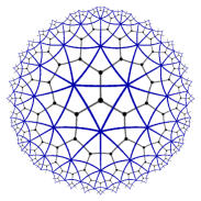
In this work, we overcome some of these challenges by applying highly efficient contraction techniques developed for matchgate tensors Valiant (2002a); Bravyi (2009), which replace tensor contraction by a Grassmann-variate integration scheme. These techniques allow us to comprehensively study the interplay of geometry and correlations in Gaussian fermionic tensor networks in a versatile fashion, incorporating toy models for quantum error correction and tensor network approaches for conformal field theory (CFT), such as the MERA, into a single framework, highlighting the connections between them. Furthermore, this framework includes highly symmetrical tensor networks based on regular tilings (see Fig. 1). We are thus in a position to efficiently probe the full space of Gaussian bulk-boundary correspondences from a small set of parameters, including the bulk curvature. We show that matchgate tensor networks with a variety of bulk geometries contain the Ising CFT in their parameter space to remarkably good approximation as a special case, with properties similar to the wavelet MERA model Evenbly and White (2016); Haegeman et al. (2018). While regular hyperbolic tilings have recently been considered as a MERA alternative Evenbly (2017), we show that flat tilings can lead to very similar boundary states. In our studies, we restrict ourselves to tensor networks that are non-unitary and real, resembling a Euclidean evolution from bulk to boundary. In particular, we do not require the causal constraints of the MERA for efficient contraction, thus providing new approaches in the context of tensor network renormalization Evenbly and Vidal (2015a, b). While we provide significant evidence that tensor networks are capable of describing bulk/boundary correspondences beyond known models and introduce a framework for their study, our work is by no means exhaustive. We do hope to provide a starting point for more systematic studies of holography in tensor networks.
Refer to caption
Refer to caption
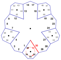
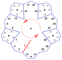
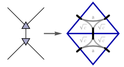
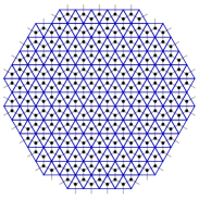
Figure 1: Triangular tilings of flat and hyperbolic space (blue edges) and the corresponding tensor network (black lattice). In the matchgate formalism, joint edges between triangles correspond to an integration over a pair of Grassmann numbers, analogous to tensor network contraction over indices.

Setting.

We construct two-dimensional planar tensor networks with fermionic bulk and boundary degrees of freedom. The bulk degrees of freedom are associated with a set V𝑉V of vertices of a tensor network. At each vertex vV𝑣𝑉v\,{\in}\,V, a local tensor Tvsubscript𝑇𝑣T_{v} with kvsubscript𝑘𝑣k_{v} indices is placed, which can be interpreted as a local fermionic state on kvsubscript𝑘𝑣k_{v} sites. After contraction over all connected bulk indices, the L𝐿L remaining open indices are interpreted as boundary sites, with the boundary state specified by the full contracted tensor. Due to the planarity of the network, the boundary sites form a loop. The bulk geometry can be flat or negatively curved (a positively curved network closes in on itself after finite distance). We visualize our tensor networks by representing each tensor Tvsubscript𝑇𝑣T_{v} as a kvsubscript𝑘𝑣k_{v}-gon whose edges correspond to indices. Thus, the tensor network is represented by a polygon tiling which determines the bulk geometry. Adjacent edges between two polygons correspond to contracted indices and boundary edges to open ones. See Fig. 1 for examples.

Concretely, each bulk degree of freedom vV𝑣𝑉v\,{\in}\,V is associated with a local tensor Tv:{0,1}×r:subscript𝑇𝑣superscript01absent𝑟T_{v}:\{0,1\}^{\times r}\,{\to}\,\mathbb{C} of tensor rank r𝑟r (equal to the number of edges of the corresponding tile), which are contracted to form tensors of higher rank. We denote the tensor component at indices j{0,1}×r𝑗superscript01absent𝑟j\,{\in}\,\{0,1\}^{\times r} as Tv(j)subscript𝑇𝑣𝑗T_{v}(j) and the standard computational basis for r𝑟r boundary spins as |jk=1r|jk\left.\left|{j}\right.\right\rangle\,{\coloneqq}\,\otimes_{k=1}^{r}\left.\left|{j_{k}}\right.\right\rangle. Each tensor is then equivalent to a state

|ψv=j{0,1}×rTv(j)|j .ketsubscript𝜓𝑣subscript𝑗superscript01absent𝑟subscript𝑇𝑣𝑗ket𝑗 .\displaystyle\left.\left|{\psi_{v}}\right.\right\rangle=\sum_{j\in\{0,1\}^{\times r}}T_{v}(j)\left.\left|{j}\right.\right\rangle\text{ .} (1)

For a broader introduction to tensor networks and their contractions, see Refs. Orus (2014); Schuch (2013); Verstraete et al. (2008); Eisert (2013).

Matchgate tensors.

Instead of explicit tensor contraction along pairs of indices, we use the formalism from Ref. Bravyi (2009) employing Grassmann integration. Any tensor T𝑇T can be represented by a Grassmann-variate characteristic function

ΦT(θ)=j{0,1}×rT(j)θ1j1θ2j2θrjr ,subscriptΦ𝑇𝜃subscript𝑗superscript01absent𝑟𝑇𝑗superscriptsubscript𝜃1subscript𝑗1superscriptsubscript𝜃2subscript𝑗2superscriptsubscript𝜃𝑟subscript𝑗𝑟 ,\displaystyle\Phi_{T}(\theta)=\sum_{j\in{\{0,1\}^{\times r}}}T(j)\theta_{1}^{j_{1}}\theta_{2}^{j_{2}}\ldots\theta_{r}^{j_{r}}\text{ ,} (2)

where the θksubscript𝜃𝑘\theta_{k} are Grassmann numbers defined by the anti-commutation relation θkθk+θkθk= 0subscript𝜃𝑘subscript𝜃superscript𝑘subscript𝜃superscript𝑘subscript𝜃𝑘 0\theta_{k}\theta_{k^{\prime}}+\theta_{k^{\prime}}\theta_{k}\,{=}\,0. The contraction T12subscript𝑇12T_{1\star 2} of two tensors T1subscript𝑇1T_{1} and T2subscript𝑇2T_{2} (of rank r1subscript𝑟1r_{1} and r2subscript𝑟2r_{2}, respectively) over the last index of T1subscript𝑇1T_{1} and the first index of T2subscript𝑇2T_{2} is given by

T12(x,y)=z{0,1}T1(x,z)T2(z,y) ,subscript𝑇12𝑥𝑦subscript𝑧01subscript𝑇1𝑥𝑧subscript𝑇2𝑧𝑦 ,T_{1\star 2}(x,y)=\sum_{z\in\{0,1\}}T_{1}(x,z)T_{2}(z,y)\text{ ,} (3)

where x{0,1}×(r11),y{0,1}×(r21)formulae-sequence𝑥superscript01absentsubscript𝑟11𝑦superscript01absentsubscript𝑟21x\,{\in}\,{\{0,1\}^{\times(r_{1}-1)}},y\,{\in}\,{\{0,1\}^{\times(r_{2}-1)}}. Clearly, T12subscript𝑇12T_{1\star 2} has rank r1+r22subscript𝑟1subscript𝑟22r_{1}+r_{2}-2. The characteristic function of the contraction is obtained as

ΦT12(ξ)=dη1dθr1ΦT1(θ)ΦT2(η)exp(θr1η1) ,subscriptΦsubscript𝑇12𝜉differential-dsubscript𝜂1differential-dsubscript𝜃subscript𝑟1subscriptΦsubscript𝑇1𝜃subscriptΦsubscript𝑇2𝜂subscript𝜃subscript𝑟1subscript𝜂1 ,\displaystyle\Phi_{T_{1\star 2}}(\xi)=\int{\rm d}\eta_{1}\int{\rm d}\theta_{r_{1}}\;\Phi_{T_{1}}(\theta)\Phi_{T_{2}}(\eta)\exp(\theta_{r_{1}}\eta_{1})\text{ ,} (4)

where we have used ξ=(θ1,,θr11,η2,,ηr2)𝜉subscript𝜃1subscript𝜃subscript𝑟11subscript𝜂2subscript𝜂subscript𝑟2\xi\,{=}\,(\theta_{1},\ldots,\theta_{r_{1}-1},\eta_{2},\ldots,\eta_{r_{2}}), and dη1dθr1differential-dsubscript𝜂1differential-dsubscript𝜃subscript𝑟1\int{\rm d}\eta_{1}\int{\rm d}\theta_{r_{1}} denotes Grassmann integrals, anti-commuting multilinear functionals obeying dξjξjzj=δzj,1differential-dsubscript𝜉𝑗superscriptsubscript𝜉𝑗subscript𝑧𝑗subscript𝛿subscript𝑧𝑗1\int{\rm d}\xi_{j}\,\xi_{j}^{z_{j}}\,{=}\,\delta_{z_{j},1} (see Refs. Berezin (1966); Cahill and Glauber (1999); Bravyi (2009, 2005) for more details). A self-contained derivation of the equivalence of (4) with tensor contraction, as well as a note on iterated integrals, is given in Appendix A. Anti-commutativity requires an appropriate labeling of all Grassmann variables, but such a labeling can always be found for contractions of planar networks Bravyi (2009). Such Grassmann integrations are particularly efficient to compute for the case of matchgate tensors, where their computation scales polynomially in the number of tensor indices.

Consider a rank-r𝑟r tensor T(x)𝑇𝑥T(x) with inputs x{0,1}×r𝑥superscript01absent𝑟x\,{\in}\,{\{0,1\}^{\times r}}. We call T(x)𝑇𝑥T(x) a matchgate if there exist an antisymmetric matrix Ar×r𝐴superscript𝑟𝑟A\,{\in}\,\mathbb{C}^{r\times r} and a z{0,1}×r𝑧superscript01absent𝑟z\,{\in}\,{\{0,1\}^{\times r}} so that we can write

T(x)=Pf(A|xXORz)T(z) ,T(x)=\mathrm{Pf}\left(A_{|x\ \texttt{XOR}\ z}\right)T(z)\text{ ,} (5)

where Pf(A)Pf𝐴\mathrm{Pf}\left(A\right) is the Pfaffian of A𝐴A, and A|xA_{|x} is the principal submatrix of A𝐴A acting on the subspace supported by x𝑥x. Furthermore, we call T(x)𝑇𝑥T(x) an even tensor if T(x)= 0𝑇𝑥 0T(x)\,{=}\,0 for any x𝑥x with odd jxjsubscript𝑗subscript𝑥𝑗\sum_{j}x_{j}.

A generic even matchgate has a simple Gaussian characteristic function of the form

ΦT(θ)=T(0)exp(12j,k=1rAj,kθjθk) ,subscriptΦ𝑇𝜃𝑇012superscriptsubscript𝑗𝑘1𝑟subscript𝐴𝑗𝑘subscript𝜃𝑗subscript𝜃𝑘 ,\Phi_{T}(\theta)=T(0)\exp\biggl{(}\frac{1}{2}\sum_{j,k=1}^{r}A_{j,k}\theta_{j}\theta_{k}\biggr{)}\ \text{ ,} (6)

where T(0)𝑇0T(0), the tensor component for all-zero input, acts as a normalization factor. Apart from normalization, the full tensor is completely determined by A𝐴A, which we therefore call the generating matrix. Thus, the rules for contracting matchgate tensors can be written as rules for combining generating matrices. Full derivations of these, including the calculation of physical covariance matrices from the generating matrices, are provided in Appendices C and D. With our contraction rules, the computational cost of contracting two tensors is quadratic in the number of indices of the final tensor. Thus, we can bound the total computational cost for contracting an entire network of the type considered here by O(L2N)𝑂superscript𝐿2𝑁O(L^{2}N), where L𝐿L is the number of boundary sites and N𝑁N is the number of contracted tensors (for similar bounds on matchgate contraction, see Ref. Bravyi (2009)).

Using Pauli matrices σαsuperscript𝜎𝛼\sigma^{\alpha} with α{x,y,z}𝛼𝑥𝑦𝑧\alpha\,{\in}\,\left\{x,y,z\right\}, we can define Majorana operators γisubscript𝛾𝑖\operatorname{\gamma}_{i} via the Jordan-Wigner transformation

γ2k1subscript𝛾2𝑘1\displaystyle{\operatorname{\gamma}}_{2k-1} =(σz)(k1)σx(𝟙2)(rk) ,absenttensor-productsuperscriptsuperscript𝜎𝑧tensor-productabsent𝑘1superscript𝜎𝑥superscriptsubscript12tensor-productabsent𝑟𝑘 ,\displaystyle=({\sigma^{z}})^{{\otimes}(k-1)}{\otimes}\,\sigma^{x}\,{\otimes}\left(\mathds{1}_{2}\right)^{\otimes(r-k)}\text{ ,} (7)
γ2ksubscript𝛾2𝑘\displaystyle{\operatorname{\gamma}}_{2k} =(σz)(k1)σy(𝟙2)(rk) .absenttensor-productsuperscriptsuperscript𝜎𝑧tensor-productabsent𝑘1superscript𝜎𝑦superscriptsubscript12tensor-productabsent𝑟𝑘 .\displaystyle=({\sigma^{z}})^{{\otimes}(k-1)}{\otimes}\,\sigma^{y}\,{\otimes}\left(\mathds{1}_{2}\right)^{\otimes(r-k)}\text{ .} (8)

The computational basis is then equivalent to an occupational basis. In this context, we prove in Appendix B that any fermionic Gaussian state vector in the form (1) has coefficients T(j)𝑇𝑗T(j) constituting a matchgate tensor. The converse is also true, providing a further perspective on the connection to free fermions Terhal and DiVincenzo (2002).

The holographic pentagon code.

We will now apply our framework to the highly symmetric class of regular bulk tilings, first implementing the holographic error correcting code (HaPPY code) proposed in Ref. Pastawski et al. (2015) and then exploiting the versatility of our framework to extend it towards more physical setups. The HaPPY code furnishes a mapping between additional (uncontracted) bulk degrees of freedom on each tensor and the boundary state, realized by a bulk tiling of pentagons. Each pentagon tile encodes one fault-tolerant logical qubit via the encoding isometry of the five qubit code. This [[5,1,3]]delimited-[]513[[5,1,3]] quantum error-correcting code Laflamme et al. (1996) saturates both the quantum Hamming bound Gottesman (1996); Terhal (2015) as well as the singleton bound Terhal (2015) and can be expressed as a stabilizer code Gottesman (1997).

We observe that fixing the bulk degrees of freedom to computational basis states gives rise to a matchgate tensor network, as the logical computational basis states of the holographic pentagon code can be viewed as ground states of a quadratic fermionic Hamiltonian. This can be seen directly by applying (7) onto the stabilizers Sksubscript𝑆𝑘S_{k} of the underlying [[5,1,3]]delimited-[]513[[5,1,3]] code, thus expressing it in terms of Majorana operators γisubscript𝛾𝑖\operatorname{\gamma}_{i} and a total parity operator 𝒫tot=(σz)5subscript𝒫totsuperscriptsuperscript𝜎𝑧tensor-productabsent5\mathcal{P}_{\text{tot}}=(\sigma^{z})^{\otimes 5}:

S1subscript𝑆1\displaystyle S_{1} =σxσzσzσx𝟙2=iγ7γ2 ,absenttensor-productsuperscript𝜎𝑥superscript𝜎𝑧superscript𝜎𝑧superscript𝜎𝑥subscript12isubscript𝛾7subscript𝛾2 ,\displaystyle=\sigma^{x}\otimes\sigma^{z}\otimes\sigma^{z}\otimes\sigma^{x}\otimes\mathds{1}_{2}=\,\mathrm{i}\operatorname{\gamma}_{7}\operatorname{\gamma}_{2}\text{ ,} (9)
S2subscript𝑆2\displaystyle S_{2} =𝟙2σxσzσzσx=iγ9γ4 ,absenttensor-productsubscript12superscript𝜎𝑥superscript𝜎𝑧superscript𝜎𝑧superscript𝜎𝑥isubscript𝛾9subscript𝛾4 ,\displaystyle=\mathds{1}_{2}\otimes\sigma^{x}\otimes\sigma^{z}\otimes\sigma^{z}\otimes\sigma^{x}=\,\mathrm{i}\operatorname{\gamma}_{9}\operatorname{\gamma}_{4}\text{ ,}
S3subscript𝑆3\displaystyle S_{3} =σx𝟙2σxσzσz=i𝒫totγ6γ1 ,absenttensor-productsuperscript𝜎𝑥subscript12superscript𝜎𝑥superscript𝜎𝑧superscript𝜎𝑧isubscript𝒫totsubscript𝛾6subscript𝛾1 ,\displaystyle=\sigma^{x}\otimes\mathds{1}_{2}\otimes\sigma^{x}\otimes\sigma^{z}\otimes\sigma^{z}=\,\mathrm{i}\,\mathcal{P}_{\text{tot}}\operatorname{\gamma}_{6}\operatorname{\gamma}_{1}\text{ ,}
S4subscript𝑆4\displaystyle S_{4} =σzσx𝟙2σxσz=i𝒫totγ8γ3 ,absenttensor-productsuperscript𝜎𝑧superscript𝜎𝑥subscript12superscript𝜎𝑥superscript𝜎𝑧isubscript𝒫totsubscript𝛾8subscript𝛾3 ,\displaystyle=\sigma^{z}\otimes\sigma^{x}\otimes\mathds{1}_{2}\otimes\sigma^{x}\otimes\sigma^{z}=\,\mathrm{i}\,\mathcal{P}_{\text{tot}}\operatorname{\gamma}_{8}\operatorname{\gamma}_{3}\text{ ,}
S5subscript𝑆5\displaystyle S_{5} =σzσzσx𝟙2σx=i𝒫totγ10γ5 .absenttensor-productsuperscript𝜎𝑧superscript𝜎𝑧superscript𝜎𝑥subscript12superscript𝜎𝑥isubscript𝒫totsubscript𝛾10subscript𝛾5 .\displaystyle=\sigma^{z}\otimes\sigma^{z}\otimes\sigma^{x}\otimes\mathds{1}_{2}\otimes\sigma^{x}=\,\mathrm{i}\,\mathcal{P}_{\text{tot}}\operatorname{\gamma}_{10}\operatorname{\gamma}_{5}\text{ .}

As the corresponding stabilizer Hamiltonian is given by H=k=15Sk𝐻superscriptsubscript𝑘15subscript𝑆𝑘H=-\sum_{k=1}^{5}S_{k}, we find a doubly degenerate ground state whose degeneracy is lifted by the parity operator 𝒫totsubscript𝒫tot\mathcal{P}_{\text{tot}}. The resulting two states with parity eigenvalues ±1plus-or-minus1\pm 1 correspond to the logical eigenstates 0¯¯0\bar{0} and 1¯¯1\bar{1}, which are themselves ground states of purely quadratic Hamiltonians with different parity factors. Thus both computational basis states are pure Gaussian, leading us to the conclusion that for fixed computational input in the bulk, the holographic pentagon code yields a matchgate tensor on the boundary (see Fig. 2). The explicit construction is given in Appendix E.5. Using the Schläfli symbol {p,q}𝑝𝑞\{p,q\}, where p𝑝p is the number of edges per polygon and q𝑞q the number of polygons around each corner, we can specify the hyperbolic geometry of the HaPPY model as a regular {5,4}54\{5,4\} tiling.

Refer to caption=Refer to captionRefer to captionRefer to caption\begin{gathered}\includegraphics[width=86.72267pt]{Figs/pentagons_hyp_code.pdf}\end{gathered}\scalebox{1.5}{$\;=\;$}\begin{gathered}\includegraphics[width=86.72267pt]{Figs/pentagons_hyp.pdf}\end{gathered}
Figure 2: The HaPPY code for fixed bulk inputs (left) is equal to a matchgate tensor network on a hyperbolic pentagon tiling (right).

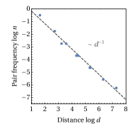
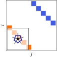
We find that the correlation structure of this model is best captured in the Majorana picture. Explicitly, consider the pentagon tiling of Ref. Pastawski et al. (2015) with all bulk inputs set to the positive-parity eigenvector |0¯ket¯0|\bar{0}\rangle. The entries of the Majorana covariance matrix Γi,j=i2ψ|[γi,γj]|ψsubscriptΓ𝑖𝑗i2quantum-operator-product𝜓subscript𝛾𝑖subscript𝛾𝑗𝜓\Gamma_{i,j}=\frac{\,\mathrm{i}\,}{2}\langle\psi|\left[\operatorname{\gamma}_{i},\operatorname{\gamma}_{j}\right]|\psi\rangle resulting from successive contraction steps are shown in Fig. 3. As we can see, both the individual pentagon state and the larger contracted states are characterized by a non-local pairing of Majorana fermions. Intriguingly, the contractions effectively connect Majorana pairs from each pentagon to a larger chain, so the pairs on the boundary of the contracted network can be seen as endpoints of a discretized “geodesic” spanning the bulk. While this discontinuous correlation pattern of Γi,jsubscriptΓ𝑖𝑗\Gamma_{i,j} makes the computation of CFT observables difficult, we can estimate the average correlation falloff by counting the relative frequency n(d)𝑛𝑑n(d) of Majorana pairs at distance d=|ij|𝑑𝑖𝑗d=|i-j| over which they connect points on the boundary. According to the results shown in Fig. 4 (left), correlation falloff follows a power law n(d)d1proportional-to𝑛𝑑superscript𝑑1n(d)\propto d^{-1}, as expected of a CFT. Furthermore, we compute the entanglement entropy SAsubscript𝑆𝐴S_{A} of a subsystem A𝐴A of size \ell averaged over all boundary positions, defined as

𝔼(S)=k=1LS[k,k+] .subscript𝔼𝑆superscriptsubscript𝑘1𝐿subscript𝑆𝑘𝑘 .\mathbb{E}_{\ell}(S)=\sum_{k=1}^{L}S_{[k,k+\ell]}\text{ .} (10)

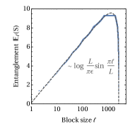
The result, shown in Fig. 4 (right), closely follows the Calabrese-Cardy formula for periodic 1+1111{+}1-dimensional CFTs, given by Holzhey et al. (1994); Calabrese and Cardy (2004)

SA=c3log(LπϵsinπL)c3logϵ+O((/L)2) ,subscript𝑆𝐴𝑐3𝐿𝜋italic-ϵ𝜋𝐿similar-to-or-equals𝑐3italic-ϵ𝑂superscript𝐿2 ,S_{A}=\frac{c}{3}\log\left(\frac{L}{\pi\epsilon}\sin\frac{\pi\ell}{L}\right)\simeq\frac{c}{3}\log\frac{\ell}{\epsilon}+O\left((\ell/L)^{2}\right)\text{ ,} (11)

with a numerical fit yielding c4.2𝑐4.2c\approx 4.2 and ϵ1.1italic-ϵ1.1\epsilon\approx 1.1 for a cutoff at L=2605𝐿2605L=2605 boundary sites.

The peculiar pair-wise correlation of boundary Majorana modes, suggesting a connection to Majorana dimer models Ware et al. (2016), will be more rigorously explored in the future. However, as the correlation structure clearly breaks the translation and scale invariance expected of CFT ground states, we now consider regular tilings with generic matchgate input.
Refer to caption
Refer to caption
Refer to caption
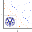
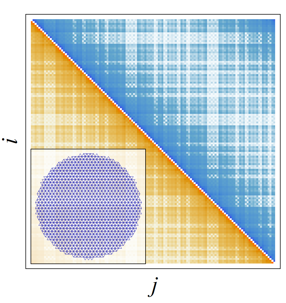
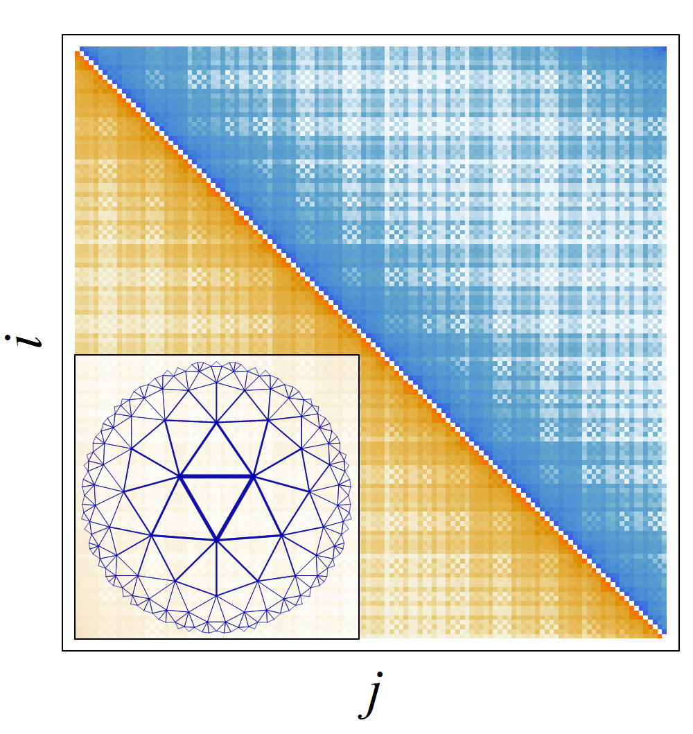
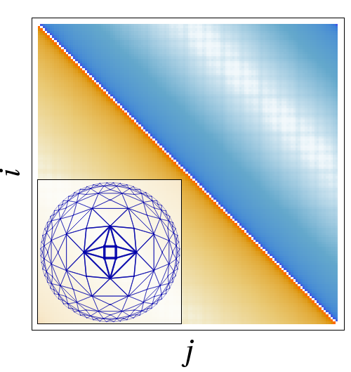
Figure 3: Majorana covariance matrix ΓΓ\Gamma for a boundary state of a pentagon tiling with 10, 40, and 50 boundary Majorana fermions (left to right). Entries Γi,jsubscriptΓ𝑖𝑗\Gamma_{i,j} are color-coded (orange = +11+1, blue = 11-1). The corresponding tiling/tensor network is shown in the lower left corner.
Refer to caption
Refer to caption
Figure 4: Boundary state properties of the HaPPY code at 2605 boundary sites. Left: Average correlations at boundary distance d𝑑d, computed as the relative frequency n𝑛n of Majorana pairs. Dashed gray line shows an n(d)1/dsimilar-to𝑛𝑑1𝑑n(d)\sim 1/d numerical fit. Right: Scaling of average entanglement entropy 𝔼(S)subscript𝔼𝑆\mathbb{E}_{\ell}(S) with subsystem size \ell. Dashed gray line shows numerical fit using (11).

Regular triangulations.

As the boundary states of triangular tilings are necessarily Gaussian Bravyi (2009), we can study their properties comprehensively using matchgate tensors. The simplest such tilings are regular and isotropic, i.e. with each local tensor specified by the same antisymmetric 3× 3333\,{\times}\,3 generating matrix A𝐴A. Isotropy constrains its components to one parameter a=A1,2=A1,3=A2,3𝑎subscript𝐴12subscript𝐴13subscript𝐴23a\,{=}\,A_{1,2}\,{=}\,A_{1,3}\,{=}\,A_{2,3}. The bulk topology follows from our choice of tiling. For triangular tilings (p= 3𝑝3p\,{=}\,3), setting q= 6𝑞6q\,{=}\,6 produces a flat tiling, whereas q> 6𝑞6q\,{>}\,6 leads to a hyperbolic one (see Fig. 1). Triangular tilings with q< 6𝑞6q\,{<}\,6 produce closed polyhedra that are positively curved and lack the notion of an asymptotic boundary. As a convention, we choose the local orientation of the triangles so that the generating matrix for the contracted boundary state satisfies Ai,j> 0subscriptsuperscript𝐴𝑖𝑗 0A^{\prime}_{i,j}\,{>}\,0 for i>j𝑖𝑗i\,{>}\,j, corresponding to anti-periodic boundary conditions: Covariance matrix entries Γi,jsubscriptΓ𝑖𝑗\Gamma_{i,j} acquire a sign flip when cyclic permutions push either index i𝑖i or j𝑗j over the boundary, as relative ordering is reversed.

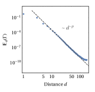
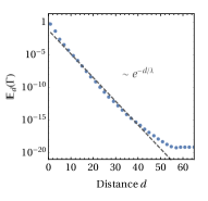
We now consider the boundary states of {3,k}3𝑘\{3,k\} bulk tilings. The falloff of correlations along the boundary generally depends on k𝑘k, i.e. the bulk curvature, as shown in Fig. 5 (top row) for the a= 0.25𝑎0.25a\,{=}\,0.25 case. While correlations between the boundary Majorana fermions of a flat bulk fall off exponentially, a hyperbolic bulk produces a polynomial decay (up to finite-size effects at large distances and rounding errors at very small correlations). In the hyperbolic case, geodesics between boundary points scale logarithmically in boundary distance, so the falloff is still exponential in bulk distance, as we would expect in AdS/CFT Balasubramanian and Ross (2000).
Refer to caption
Refer to caption
Refer to caption
Refer to caption
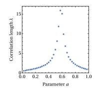
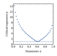
Figure 5: Top: Mean value of Majorana covariance 𝔼d(Γ)=subscript𝔼𝑑Γabsent\mathbb{E}_{d}(\Gamma)\,{=}\, k=1L|Γk,k+d|/Lsuperscriptsubscript𝑘1𝐿subscriptΓ𝑘𝑘𝑑𝐿\sum_{k=1}^{L}|\Gamma_{k,k+d}|/L (with Γi,L+j=Γi,jsubscriptΓ𝑖𝐿𝑗subscriptΓ𝑖𝑗\Gamma_{i,L+j}\,{=}\,\Gamma_{i,j}) at boundary distance d𝑑d. For {3,6}36\{3,6\} tiling with 150 boundary Majorana fermions (left) and {3,7}37\{3,7\} tiling with 348 (right). a= 0.25𝑎0.25a\,{=}\,0.25 in both cases. Bottom: Dependence of correlation falloff on a𝑎a, for {3,6}36\{3,6\} tiling with falloff ed/λsimilar-toabsentsuperscript𝑒𝑑𝜆\sim e^{-d/\lambda} (left) and {3,7}37\{3,7\} tiling with dpproportional-toabsentsuperscript𝑑𝑝\propto d^{-p} (right).
Refer to caption
Refer to caption
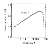
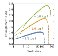
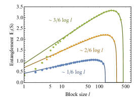
Figure 6: Average entanglement entropy 𝔼(S)subscript𝔼𝑆\mathbb{E}_{\ell}(S) of a boundary subsystem with size \ell, numerical data and exact CFT solutions (11) (dashed lines). Left: Results for {3,6}36\{3,6\} tiling (blue) at a=0.580𝑎0.580a=0.580 and {3,7}37\{3,7\} tiling (yellow) at a=0.609𝑎0.609a=0.609 (for 348 Majorana sites each). Right: {3,8}38\{3,8\} tiling with bond dimension χ=2,4,8𝜒248\chi=2,4,8 on 144, 288, and 432 sites, respectively.

Restricting ourselves to the 0a 10𝑎10\,{\leq}\,a\,{\leq}\,1 region, we explore how quickly correlations decay in both settings. At a= 0𝑎 0a\,{=}\,0 and a= 1𝑎1a\,{=}\,1, the boundary Majorana fermions only have neighboring pair correlations, either pairing within each edge (a= 0𝑎 0a\,{=}\,0) or across the corners (a= 1𝑎1a\,{=}\,1). Thus correlation decay becomes infinite in the limits a 0𝑎 0a\,{\to}\,0 and a 1𝑎1a\,{\to}\,1, independent of bulk geometry. We use numerical fits to study the remaining region 0<a< 10𝑎10\,{<}\,a\,{<}\,1 (see Fig. 5, bottom row). For a hyperbolic bulk geometry the power law is generic with the slowest decay at a 0.61𝑎0.61a\,{\approx}\,0.61, where we see a d1proportional-toabsentsuperscript𝑑1\propto d^{-1} falloff over distance d𝑑d. The exponential decay ed/λproportional-toabsentsuperscript𝑒𝑑𝜆\propto e^{-d/\lambda} generally produced by a flat bulk geometry, however, slows down to a power law (with correlation length λ𝜆\lambda diverging) around a 0.58𝑎0.58a\,{\approx}\,0.58, where correlations again decay as d1proportional-toabsentsuperscript𝑑1\propto d^{-1}. At their critical values, the boundary states of both bulk geometries have the same average properties.

Parameter Exact {3,6}36\{3,6\} bulk {3,7}37\{3,7\} bulk mMERA Wavelets
ϵ0subscriptitalic-ϵ0\epsilon_{0} 0.63660.6366-0.6366 0.61390.6139-0.6139 0.56170.5617-0.5617 0.63650.6365-0.6365 0.62110.6211-0.6211
c𝑐c 0.50000.5000\phantom{-}0.5000 0.50060.5006\phantom{-}0.5006 0.50180.5018\phantom{-}0.5018 0.49580.4958\phantom{-}0.4958 0.49570.4957\phantom{-}0.4957
Δψ,Δψ¯subscriptΔ𝜓subscriptΔ¯𝜓\Delta_{\psi},\Delta_{\bar{\psi}} 0.50000.5000\phantom{-}0.5000 0.49480.4948\phantom{-}0.4948 0.49510.4951\phantom{-}0.4951 0.50230.5023\phantom{-}0.5023 0.50000.5000\phantom{-}0.5000
ΔϵsubscriptΔitalic-ϵ\Delta_{\epsilon} 1.00001.0000\phantom{-}1.0000 0.98560.9856\phantom{-}0.9856 1.01211.0121\phantom{-}1.0121 1.00271.0027\phantom{-}1.0027 1.00001.0000\phantom{-}1.0000
ΔσsubscriptΔ𝜎\Delta_{\sigma} 0.12500.1250\phantom{-}0.1250 0.14030.1403\phantom{-}0.1403 0.13680.1368\phantom{-}0.1368 0.14170.1417\phantom{-}0.1417 0.14020.1402\phantom{-}0.1402
Cσ,σ,ϵsubscript𝐶𝜎𝜎italic-ϵC_{\sigma,\sigma,\epsilon} 0.50000.5000\phantom{-}0.5000 0.54700.5470\phantom{-}0.5470 0.53360.5336\phantom{-}0.5336 0.51560.5156\phantom{-}0.5156 0.45840.4584\phantom{-}0.4584
Table 1: Table of conformal data for the regular {3,6}36\{3,6\} and {3,7}37\{3,7\} bulk tilings as well as the mMERA, compared to the exact results and the wavelet MERA Evenbly and White (2016). Listed are the ground-state energy density ϵ0subscriptitalic-ϵ0\epsilon_{0}, central charge c𝑐c, scaling dimensions ΔϕsubscriptΔitalic-ϕ\Delta_{\phi} of the fields ϕ=ψ,ψ¯,ϵ,σitalic-ϕ𝜓¯𝜓italic-ϵ𝜎\phi=\psi,\bar{\psi},\epsilon,\sigma, and the structure constant Cσ,σ,ϵsubscript𝐶𝜎𝜎italic-ϵC_{\sigma,\sigma,\epsilon}. The non-scaling of the identity 𝟙1\mathds{1} is discussed in Appendix E.3.

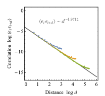
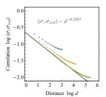
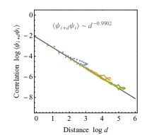
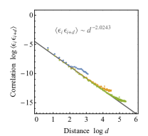
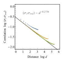
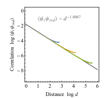
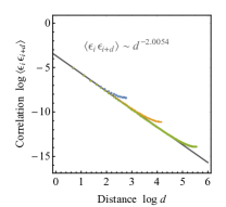
Up to finite-size effects, this critical boundary theory turns out to be the Ising CFT, as we confirm by computing a range of critical properties from the covariance matrix, shown in Table 1. The entanglement entropy scaling, shown in Fig. 6 (left), again matches the expected form (11) irrespective of the choice of tiling. The Ising CFT state that we observe at the critical value of a𝑎a is the ground state of the Hamiltonian

H=i(i=1N1γiγi+1+γ1γN) ,𝐻isuperscriptsubscript𝑖1𝑁1subscript𝛾𝑖subscript𝛾𝑖1subscript𝛾1subscript𝛾𝑁 ,H=\,\mathrm{i}\left(\sum_{i=1}^{N-1}\operatorname{\gamma}_{i}\operatorname{\gamma}_{i+1}+\operatorname{\gamma}_{1}\operatorname{\gamma}_{N}\right)\text{ ,} (12)

where the sign of the boundary term γ1γNsubscript𝛾1subscript𝛾𝑁\operatorname{\gamma}_{1}\operatorname{\gamma}_{N} signifies anti-periodic boundary conditions. Triangular tilings also incorporate more generic models: By associating each edge with a bond dimension χ> 2𝜒2\chi\,{>}\,2, it is possible to produce boundary theories with central charges in multiples of 1/2121/2, as laid out in Appendix E.6 and shown in Fig. 6 (right). Furthermore, by changing the tensor content in a central region of the network, a mass gap can be introduced, highlighting how radii in a hyperbolic bulk correspond to a renormalization scale on the boundary. Details are provided in Appendix E.4.

Translation invariance and MERA.

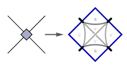
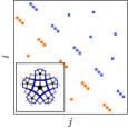
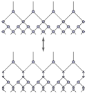
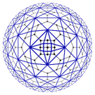
The regular bulk tilings considered so far possess a set of discrete symmetries. When choosing identical tensors on each polygon, the boundary states neccessarily inherit these symmetries, breaking translation invariance. To recover it, we consider a tiling with the same geometry as the MERA network. As we restrict ourselves to real generating matrices for the 3- and 4-leg matchgate tensors in this geometry, our model is not a unitary circuit but a model of Euclidean entanglement renormalization resembling imaginary time evolution, extending ideas from Refs. Evenbly and Vidal (2015a, b). This may provide a more realistic representation of the causal structure of an AdS time-slice than the standard MERA. Accordingly, the tensors of our matchgate MERA (mMERA) do not correspond to the usual (norm-preserving) isometries and disentanglers. Remarkably, we can still produce almost perfectly translation-invariant boundary states (Fig. 8) while optimizing over only three parameters and recover the expected CFT properties (Table 1). In particular, at bond dimension χ= 2𝜒2\chi\,{=}\,2 the ground-state energy has a relative error of only 0.02%percent0.020.02\% compared to the exact solution. Note that the optimization process only takes a few minutes on a desktop computer for a network with hundreds of tensors. We also find that the χ= 2𝜒2\chi\,{=}\,2 mMERA possesses a symmetry that allows us to write its 4-leg tensors as contractions of simpler 3-leg tensors (see Fig. 7), yielding a non-regular triangular tiling. Whether alternating or quasi-periodic tilings with a larger parameter space than regular tilings can also produce translation-invariant states is an interesting open question.
Refer to caption
Refer to caption
Figure 7: Left: Mapping between standard MERA tensor network and a network of 3-leg tensors. Right: Mapping of the corresponding mMERA network onto a triangular tiling in the Poincaré disk.
Refer to caption
Refer to caption
Refer to caption
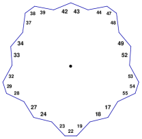
Figure 8: Color-coded entries of the field correlation matrix ψiψj=(Γ2i,2j1+Γ2i1,2j)/4delimited-⟨⟩subscript𝜓𝑖subscript𝜓𝑗subscriptΓ2𝑖2𝑗1subscriptΓ2𝑖12𝑗4\langle\psi_{i}\psi_{j}\rangle\,{=}\,(\Gamma_{2i,2j-1}+\Gamma_{2i-1,2j})/4 for boundary states of the {3,6}36\{3,6\}, {3,7}37\{3,7\} and mMERA tiling at criticality (from left to right) with 129, 126 and 128 boundary sites, respectively. The corresponding tiling is shown in the lower left corner.

Discussion

In this work, we have studied bulk-boundary correspondences in fermionic Gaussian tensor networks, introducing a versatile framework and a highly efficient contraction method based on matchgate tensors Valiant (2002a); Bravyi (2009) for a wide class of flat and hyperbolic bulk tilings. We showed that our framework includes the holographic pentagon code built from 555-qubit stabilizer states for fixed bulk inputs. Its boundary states correspond to a non-local bulk pairing of Majorana fermions, opening an avenue to studying the state properties of this holographic model at large sizes. We explicitly computed 2-point correlators and entanglement entropies, which were found to exhibit critical scaling. Beyond known models, we showed that critical and gapped Gaussian boundary states can be realized by various bulk tilings. In particular, the average scaling properties of the c= 1/2𝑐12c\,{=}\,1/2 Ising CFT (and multiples thereof) can be reproduced using regular one-parameter bulk triangulations with both flat and hyperbolic curvature. This is particularly unexpected for the flat case where boundary theories are typically gapped, and raises the question whether this appearance of criticality is retained in strongly interacting models, as well. Intriguingly, the appearance of equivalent boundary CFT states for flat and hyperbolic bulks resembles the effect of local Weyl transformations in Euclidean path-integrals Caputa et al. (2017). Furthermore, we constructed the mMERA, a Euclidean matchgate tensor network based on the MERA geometry. Beyond the results achievable with regular triangulations, this tiling - which can also be expressed as a triangulation - recovers the Ising CFT with translation invariance, while requiring only three free parameters and little computational cost. Within the Gaussian setting, further studies could focus on positively curved bulks, higher-dimensional models and random tensors. Beyond Gaussianity, our framework is extendable to interacting bulk-boundary models which can be explored with interacting fermionic tensor networks Barthel et al. (2009); Corboz et al. (2010); Kraus et al. (2010); Wille et al. (2017); Bultinck et al. (2017), yet avoiding the prohibitive computational effort of general methods for exact tensor contraction.

Acknowledgements.

We would like to thank Aleksander Kubica for pointing out that [[5,1,3]]delimited-[]513[[5,1,3]] code states Laflamme et al. (1996) are in fact ground states of quadratic Majorana Hamiltonians. We also thank Xiao-Liang Qi, Tadashi Takayanagi, and Pawel Caputa for helpful discussions. We thank the ERC (TAQ), the DFG (CRC 183, EI 519/7-1, EI 519/14-1), the Templeton Foundation, the EC (PASQuanS), the Studienstiftung, and the A.v.-Humboldt Foundation for support.

Appendix

This appendix contains additional details, technical calculations and proofs of the assertions made in the main text. We begin by showing how to perform tensor contraction using Grassmann integration in Section A, followed by a minimal example of contracting two matchgate tensors. In Section B, we restructure the definitions made in Ref. Bravyi (2009) in order to bring the theory of matchgates closer to the free fermionic formalism. In particular, we prove the correspondence between matchgate tensors and fermionic Gaussian states. In Section C, we show how to convert a generating matrix of a matchgate tensor to the covariance matrix of the corresponding state, yielding the physically relevant correlations. In Section D, we provide technical details and calculations for the contraction rules in the Grassmann formalism used in the numerical implementation. In Section E, we give explicit examples of generating matrices relevant to the main text, show the extracted critical data from the respective covariance matrices, and present a construction of states with higher central charges.

Appendix A Tensor contractions in the Grassmann formalism

In this section, we review the approach to contraction of matchgate tensor networks through Grassmann integration Bravyi (2009). In particular we present a simplified version of Lemma 5 from Ref. Bravyi (2009) and explain this result through an example. Grassmann variables will be denoted by θ𝜃\theta and are a set of anti-commuting generators of an algebra (θiθj=θjθi)subscript𝜃𝑖subscript𝜃𝑗subscript𝜃𝑗subscript𝜃𝑖(\theta_{i}\theta_{j}=-\theta_{j}\theta_{i}) which nevertheless commutes with ordinary scalars x𝑥x (xθi=θix).𝑥subscript𝜃𝑖subscript𝜃𝑖𝑥(x\theta_{i}=\theta_{i}x). A general element in this algebra may be written as

z=k=0ni1,,ikci1ikθi1θik,𝑧superscriptsubscript𝑘0𝑛subscriptsubscript𝑖1subscript𝑖𝑘subscript𝑐subscript𝑖1subscript𝑖𝑘subscript𝜃subscript𝑖1subscript𝜃subscript𝑖𝑘\displaystyle z=\sum_{k=0}^{n}\sum_{i_{1},\cdots,i_{k}}c_{i_{1}\cdots i_{k}}\theta_{i_{1}}\cdots\theta_{i_{k}}, (13)

where ci1iksubscript𝑐subscript𝑖1subscript𝑖𝑘c_{i_{1}\cdots i_{k}} can be arbitrary complex coefficients and iksubscript𝑖𝑘i_{k} form an increasing sequence in {1,2,,n}12𝑛\{1,2,\ldots,n\}. In particular, given a tensor T:{0,1}×r:𝑇superscript01absent𝑟T:{\{0,1\}^{\times r}}\rightarrow\mathbb{C} we associate to it a polynomial in Grassmann numbers given by

ΦT(θ)=j{0,1}×rT(j)θ1j1θ2j2θrjr ,subscriptΦ𝑇𝜃subscript𝑗superscript01absent𝑟𝑇𝑗superscriptsubscript𝜃1subscript𝑗1superscriptsubscript𝜃2subscript𝑗2superscriptsubscript𝜃𝑟subscript𝑗𝑟 ,\displaystyle\Phi_{T}(\theta)=\sum_{j\in{\{0,1\}^{\times r}}}T(j)\theta_{1}^{j_{1}}\theta_{2}^{j_{2}}\ldots\theta_{r}^{j_{r}}\text{ ,} (14)

which we call its characteristic function.

For simplicity, we consider contracting the last index of a rank-r1subscript𝑟1r_{1} tensor T1subscript𝑇1T_{1} with the first index of a rank-r2subscript𝑟2r_{2} tensor T2subscript𝑇2T_{2} where r1,r21subscript𝑟1subscript𝑟21r_{1},r_{2}\geq 1. Let us denote r1=r11superscriptsubscript𝑟1subscript𝑟11r_{1}^{\prime}=r_{1}-1 and r2=r21superscriptsubscript𝑟2subscript𝑟21r_{2}^{\prime}=r_{2}-1 This operation gives rise to a rank-(r1+r2)superscriptsubscript𝑟1superscriptsubscript𝑟2(r_{1}^{\prime}+r_{2}^{\prime}) tensor T12subscript𝑇12T_{1\star 2} with entries

T12(x,y)=z{0,1}T1(x,z)T2(z,y)subscript𝑇12𝑥𝑦subscript𝑧01subscript𝑇1𝑥𝑧subscript𝑇2𝑧𝑦\displaystyle T_{1\star 2}(x,y)=\sum_{z\in\{0,1\}}T_{1}(x,z)T_{2}(z,y) (15)

for x{0,1}×r1𝑥superscript01absentsuperscriptsubscript𝑟1x\in{\{0,1\}^{\times r_{1}^{\prime}}} and y{0,1}×r2𝑦superscript01absentsuperscriptsubscript𝑟2y\in{\{0,1\}^{\times r_{2}^{\prime}}} being binary words. The characteristic function for the contraction of two tensors can be obtained by

ΦT12(θ~,η~)=𝑑η1𝑑θr1ΦT1(θ)ΦT2(η)exp(θr1η1)subscriptΦsubscript𝑇12~𝜃~𝜂differential-dsubscript𝜂1differential-dsubscript𝜃subscript𝑟1subscriptΦsubscript𝑇1𝜃subscriptΦsubscript𝑇2𝜂subscript𝜃subscript𝑟1subscript𝜂1\displaystyle\Phi_{T_{1\star 2}}(\tilde{\theta},\tilde{\eta})=\int d\eta_{1}\int d\theta_{r_{1}}\;\Phi_{T_{1}}(\theta)\Phi_{T_{2}}(\eta)\exp(\theta_{r_{1}}\eta_{1}) (16)

where θ~=(θ1,,θr1)~𝜃subscript𝜃1subscript𝜃superscriptsubscript𝑟1\tilde{\theta}=(\theta_{1},\ldots,\theta_{r_{1}^{\prime}}), η~=(η1,,ηr2)~𝜂subscript𝜂1subscript𝜂superscriptsubscript𝑟2\tilde{\eta}=(\eta_{1},\ldots,\eta_{r_{2}^{\prime}}) correspond to uncontracted indices and θr1subscript𝜃subscript𝑟1\theta_{r_{1}} and η1subscript𝜂1\eta_{1} are the two Grassmann numbers of the two indices that are being contracted. Let us use exp(θr1η1)=1+θr1η1subscript𝜃subscript𝑟1subscript𝜂11subscript𝜃subscript𝑟1subscript𝜂1\exp(\theta_{r_{1}}\eta_{1})=1+\theta_{r_{1}}\eta_{1} on the right hand side

RHS=x{0,1}×r1y{0,1}×r2a,b{0,1}T1(x,a)T2(b,y)𝑑η1𝑑θr1θ1x1θ2x2θr1xr1θr1aη1bη2y1ηr2yr2(1+θr1η1)𝑅𝐻𝑆subscript𝑥superscript01absentsuperscriptsubscript𝑟1𝑦superscript01absentsuperscriptsubscript𝑟2subscript𝑎𝑏01subscript𝑇1𝑥𝑎subscript𝑇2𝑏𝑦differential-dsubscript𝜂1differential-dsubscript𝜃subscript𝑟1superscriptsubscript𝜃1subscript𝑥1superscriptsubscript𝜃2subscript𝑥2superscriptsubscript𝜃superscriptsubscript𝑟1subscript𝑥superscriptsubscript𝑟1superscriptsubscript𝜃subscript𝑟1𝑎superscriptsubscript𝜂1𝑏superscriptsubscript𝜂2subscript𝑦1superscriptsubscript𝜂subscript𝑟2subscript𝑦superscriptsubscript𝑟21subscript𝜃subscript𝑟1subscript𝜂1\displaystyle RHS=\sum_{\begin{subarray}{c}x\in{\{0,1\}^{\times r_{1}^{\prime}}}\\ y\in{\{0,1\}^{\times r_{2}^{\prime}}}\end{subarray}}\sum_{a,b\in\{0,1\}}T_{1}(x,a)T_{2}(b,y)\int d\eta_{1}\int d\theta_{r_{1}}\ \theta_{1}^{x_{1}}\theta_{2}^{x_{2}}\ldots\theta_{r_{1}^{\prime}}^{x_{r_{1}^{\prime}}}\theta_{r_{1}}^{a}\eta_{1}^{b}\eta_{2}^{y_{1}}\ldots\eta_{r_{2}}^{y_{r_{2}^{\prime}}}(1+\theta_{r_{1}}\eta_{1}) (17)

and observe that the two integrals commute with the first r11subscript𝑟11r_{1}-1 of the θ𝜃\theta’s and exponential factor commutes with the η𝜂\eta’s. This gives

RHS=x{0,1}×r1y{0,1}×r2a,b{0,1}T1(x,a)T2(b,y)θ1x1θ2x2θr1xr1[𝑑η1𝑑θr1θr1aη1b(1+θr1η1)]η2y1ηr2yr2.𝑅𝐻𝑆subscript𝑥superscript01absentsuperscriptsubscript𝑟1𝑦superscript01absentsuperscriptsubscript𝑟2subscript𝑎𝑏01subscript𝑇1𝑥𝑎subscript𝑇2𝑏𝑦superscriptsubscript𝜃1subscript𝑥1superscriptsubscript𝜃2subscript𝑥2superscriptsubscript𝜃superscriptsubscript𝑟1subscript𝑥superscriptsubscript𝑟1delimited-[]differential-dsubscript𝜂1differential-dsubscript𝜃subscript𝑟1superscriptsubscript𝜃subscript𝑟1𝑎superscriptsubscript𝜂1𝑏1subscript𝜃subscript𝑟1subscript𝜂1superscriptsubscript𝜂2subscript𝑦1superscriptsubscript𝜂subscript𝑟2subscript𝑦superscriptsubscript𝑟2\displaystyle RHS=\sum_{\begin{subarray}{c}x\in{\{0,1\}^{\times r_{1}^{\prime}}}\\ y\in{\{0,1\}^{\times r_{2}^{\prime}}}\end{subarray}}\sum_{a,b\in\{0,1\}}T_{1}(x,a)T_{2}(b,y)\theta_{1}^{x_{1}}\theta_{2}^{x_{2}}\ldots\theta_{r_{1}^{\prime}}^{x_{r_{1}^{\prime}}}\left[\int d\eta_{1}\int d\theta_{r_{1}}\ \theta_{r_{1}}^{a}\eta_{1}^{b}(1+\theta_{r_{1}}\eta_{1})\right]\;\eta_{2}^{y_{1}}\ldots\eta_{r_{2}}^{y_{r_{2}^{\prime}}}. (18)

For the middle bracket, we obtain

𝑑η1𝑑θr1θr1aη1b(1+θr1η1)=δa,bdifferential-dsubscript𝜂1differential-dsubscript𝜃subscript𝑟1superscriptsubscript𝜃subscript𝑟1𝑎superscriptsubscript𝜂1𝑏1subscript𝜃subscript𝑟1subscript𝜂1subscript𝛿𝑎𝑏\displaystyle\int d\eta_{1}\int d\theta_{r_{1}}\ \theta_{r_{1}}^{a}\eta_{1}^{b}(1+\theta_{r_{1}}\eta_{1})=\delta_{a,b} (19)

and therefore

RHS=x{0,1}×r1y{0,1}×r2[z{0,1}T1(x,z)T2(z,y)]θ1x1θ2x2θr1xr1η2y1ηr2yr2.𝑅𝐻𝑆subscript𝑥superscript01absentsuperscriptsubscript𝑟1𝑦superscript01absentsuperscriptsubscript𝑟2delimited-[]subscript𝑧01subscript𝑇1𝑥𝑧subscript𝑇2𝑧𝑦superscriptsubscript𝜃1subscript𝑥1superscriptsubscript𝜃2subscript𝑥2superscriptsubscript𝜃superscriptsubscript𝑟1subscript𝑥superscriptsubscript𝑟1superscriptsubscript𝜂2subscript𝑦1superscriptsubscript𝜂subscript𝑟2subscript𝑦superscriptsubscript𝑟2\displaystyle RHS=\sum_{\begin{subarray}{c}x\in{\{0,1\}^{\times r_{1}^{\prime}}}\\ y\in{\{0,1\}^{\times r_{2}^{\prime}}}\end{subarray}}\left[\sum_{z\in\{0,1\}}T_{1}(x,z)T_{2}(z,y)\right]\theta_{1}^{x_{1}}\theta_{2}^{x_{2}}\ldots\theta_{r_{1}^{\prime}}^{x_{r_{1}^{\prime}}}\eta_{2}^{y_{1}}\ldots\eta_{r_{2}}^{y_{r_{2}^{\prime}}}. (20)

We see that this is exactly the characteristic function for the tensor contraction. Note that it is important that we contract the last index with the first one. Lemma 5 of Ref. Bravyi (2009) generalizes this calculation to an arbitrary number of indices that are being contracted in an appropriate order – this essentially could be derived by iterating the formula that we derived for the case of self-contractions.

A.1 Minimal example

As an example, we want to show the contraction of two tensors TA,TBsubscript𝑇𝐴subscript𝑇𝐵T_{A},T_{B} with Gaussian characteristic functions of the form

ΦTA(θ)=exp(12j,k=1LAj,kθjθk),ΦTB(θ)=exp(12j,k=1LBj,kθjθk).formulae-sequencesubscriptΦsubscript𝑇𝐴𝜃12superscriptsubscript𝑗𝑘1𝐿subscript𝐴𝑗𝑘subscript𝜃𝑗subscript𝜃𝑘subscriptΦsubscript𝑇𝐵𝜃12superscriptsubscript𝑗𝑘1𝐿subscript𝐵𝑗𝑘subscript𝜃𝑗subscript𝜃𝑘\displaystyle\Phi_{T_{A}}(\theta)=\exp\biggl{(}\frac{1}{2}\sum_{j,k=1}^{L}A_{j,k}\theta_{j}\theta_{k}\biggr{)}\;,\quad\quad\Phi_{T_{B}}(\theta)=\exp\biggl{(}\frac{1}{2}\sum_{j,k=1}^{L}B_{j,k}\theta_{j}\theta_{k}\biggr{)}\;. (21)

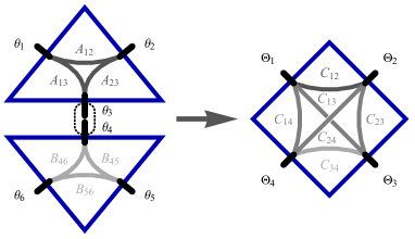
As we summarize in Fig. 9, we associate the Grassmann numbers θ1,θ2,θ3subscript𝜃1subscript𝜃2subscript𝜃3\theta_{1},\theta_{2},\theta_{3} to A𝐴A and θ4,θ5,θ6subscript𝜃4subscript𝜃5subscript𝜃6\theta_{4},\theta_{5},\theta_{6} to B𝐵B, and fix θ3subscript𝜃3\theta_{3} and θ4subscript𝜃4\theta_{4} on the edges between the triangles to be integrated out, yielding a state with four edges whose correlation matrix C𝐶C shall be computed from A𝐴A and B𝐵B via Grassmann integration

ΦC(Θ)=dθ4dθ3eθ3θ4+12j,k=16(AB)j,kθjθksubscriptΦ𝐶Θdsubscript𝜃4dsubscript𝜃3superscript𝑒subscript𝜃3subscript𝜃412superscriptsubscript𝑗𝑘16subscriptdirect-sum𝐴𝐵𝑗𝑘subscript𝜃𝑗subscript𝜃𝑘\Phi_{C}(\Theta)=\int\text{d}\theta_{4}\text{d}\theta_{3}\,e^{\theta_{3}\theta_{4}+\frac{1}{2}\sum_{j,k=1}^{6}(A\oplus B)_{j,k}\theta_{j}\theta_{k}} (22)

where Θ=(θ1,θ2,θ5,θ6)Θsuperscriptsubscript𝜃1subscript𝜃2subscript𝜃5subscript𝜃6top\Theta=(\theta_{1},\theta_{2},\theta_{5},\theta_{6})^{\top} contains the four Grassmann numbers that remain after integration. Taking A,B𝐴𝐵A,B as input, we find that after the integration ΦTCsubscriptΦsubscript𝑇𝐶\Phi_{T_{C}} is again Gaussian (the technicalities of integration will be dealt with in Section D) and the generating matrix is

C=(0A1,2A1,3B4,5A1,3B4,6A1,20A2,3B4,5A2,3B4,6A1,3B4,5A2,3B4,50B5,6A1,3B4,6A2,3B4,6B5,60) .𝐶matrix0subscript𝐴12subscript𝐴13subscript𝐵45subscript𝐴13subscript𝐵46subscript𝐴120subscript𝐴23subscript𝐵45subscript𝐴23subscript𝐵46subscript𝐴13subscript𝐵45subscript𝐴23subscript𝐵450subscript𝐵56subscript𝐴13subscript𝐵46subscript𝐴23subscript𝐵46subscript𝐵560 .C=\left(\begin{matrix}0&A_{1,2}&A_{1,3}B_{4,5}&A_{1,3}B_{4,6}\\ -A_{1,2}&0&A_{2,3}B_{4,5}&A_{2,3}B_{4,6}\\ -A_{1,3}B_{4,5}&-A_{2,3}B_{4,5}&0&B_{5,6}\\ -A_{1,3}B_{4,6}&-A_{2,3}B_{4,6}&-B_{5,6}&0\\ \end{matrix}\right)\text{ .} (23)

We observe that the newly created entries in the upper right corner are in fact a dyadic product and this block is a lower-rank matrix.
Refer to caption
Figure 9: Contraction of two triangle states with Grassmann-variable edges {θ1,θ2,θ3}subscript𝜃1subscript𝜃2subscript𝜃3\{\theta_{1},\theta_{2},\theta_{3}\} and {θ4,θ5,θ6}subscript𝜃4subscript𝜃5subscript𝜃6\{\theta_{4},\theta_{5},\theta_{6}\} into a state with four edges {Θ1,Θ2,Θ3,Θ4}subscriptΘ1subscriptΘ2subscriptΘ3subscriptΘ4\{\Theta_{1},\Theta_{2},\Theta_{3},\Theta_{4}\}.

Appendix B Matchgates and fermionic Gaussian states

We first discuss definitions of matchgate tensors and then explain the connection to fermionic Gaussian states.

B.1 Definitions of matchgates

For completeness, we shortly recapitulate the characterization of matchgates by Bravyi in Ref. Bravyi (2009). Originally matchgates Valiant (2002b) were characterized as the local tensors of a tensor network that can be contracted efficiently through the Fisher-Kastelyn-Temperley method Temperley and Fisher (1961); Kasteleyn (1961). Subsequently, the following algebraic characterization has been found Cai et al. (2007).

Definition 1 (Matchgate equations).

A rank-r𝑟r tensor T𝑇T is a matchgate if for all x,y{0,1}×r𝑥𝑦superscript01absent𝑟x,y\in{\{0,1\}^{\times r}} it holds that

k:xkykT(xXORek)T(yXORek)(1)j=1k1(xj+yj)=0subscript:𝑘subscript𝑥𝑘subscript𝑦𝑘𝑇𝑥XORsuperscript𝑒𝑘𝑇𝑦XORsuperscript𝑒𝑘superscript1superscriptsubscript𝑗1𝑘1subscript𝑥𝑗subscript𝑦𝑗0\displaystyle\sum_{k:\ x_{k}\neq y_{k}}T(x\ \texttt{XOR}\ e^{k})T(y\ \texttt{XOR}\ e^{k})(-1)^{\sum_{j=1}^{k-1}(x_{j}+y_{j})}=0 (24)

where (ek)q=δk,qsubscriptsuperscript𝑒𝑘𝑞subscript𝛿𝑘𝑞(e^{k})_{q}=\delta_{k,q}.

Proposition 2 of Ref. Bravyi (2009) shows that one can equivalently define matchgates through Pfaffians, leading to the following equivalent definition.

Definition 2 (Matchgates as Pfaffians).

A rank-r𝑟r tensor T𝑇T is a matchgate if there exists a reference index z{0,1}×r𝑧superscript01absent𝑟z\in{\{0,1\}^{\times r}} and an anti-symmetric matrix Ar×r𝐴superscript𝑟𝑟A\in\mathbb{C}^{r\times r}, such that for any x{0,1}×r𝑥superscript01absent𝑟x\in{\{0,1\}^{\times r}}

T(x)=Pf(A|xXORz)T(z).\displaystyle T(x)=\mathrm{Pf}\left(A_{|x\ \texttt{XOR}\ z}\right)T(z). (25)

In particular, A𝐴A is explicitly given by Aj,k=T(ejXORekXORz)/T(z)subscript𝐴𝑗𝑘𝑇superscript𝑒𝑗XORsuperscript𝑒𝑘XOR𝑧𝑇𝑧A_{j,k}=T(e^{j}\ \texttt{XOR}\ e^{k}\ \texttt{XOR}\ z)/T(z) for j<k𝑗𝑘j<k if T(z)0𝑇𝑧0T(z)\neq 0 or A0𝐴0A\equiv 0 if T0𝑇0T\equiv 0 and we denote by A|xXORzA_{|x\ \texttt{XOR}\ z} the restriction of A𝐴A to the entries indicated by xXORz𝑥XOR𝑧x\ \texttt{XOR}\ z.

Proof of the equivalence of these definitions. In particular, proposition 2 of Ref. Bravyi (2009) shows that whenever T(z)0𝑇𝑧0T(z)\neq 0 then a new matchgate tensor Tsuperscript𝑇T^{\prime} fulfills T(x)=T(xXORz)/T(z)=Pf(A|x)T^{\prime}(x)=T(x\ \texttt{XOR}\ z)/T(z)=\mathrm{Pf}\left(A_{|x}\right) which is derived from the matchgate equations. From this we have that T(xXORz)=T(xXORzXORz)/T(z)=T(x)/T(z)=Pf(A|xXORz)T(z)T^{\prime}(x\ \texttt{XOR}\ z)=T(x\ \texttt{XOR}\ z\ \texttt{XOR}\ z)/T(z)=T(x)/T(z)=\mathrm{Pf}\left(A_{|x\ \texttt{XOR}\ z}\right)T(z) and therefore T(x)=Pf(A|xXORz)T(z)T(x)=\mathrm{Pf}\left(A_{|x\ \texttt{XOR}\ z}\right)T(z). Finally, for the trivial matchgate tensor T=0𝑇0T=0 both definitions agree, too.

The converse direction can be shown by a simplification of the argument of Theorem 2 of Ref. Bravyi (2009). We start with T(x)=Pf(A|xXORz)T(z)T(x)=\mathrm{Pf}\left(A_{|x\ \texttt{XOR}\ z}\right)T(z). If T(z)=0𝑇𝑧0T(z)=0 then T𝑇T fulfills the matchgate equations trivially. Otherwise we consider Tsuperscript𝑇T^{\prime} with entries T(x)=T(xXORz)/T(z)=Pf(A|x)T^{\prime}(x)=T(x\ \texttt{XOR}\ z)/T(z)=\mathrm{Pf}\left(A_{|x}\right) which has a Gaussian characteristic function

ΦT(θ)=exp(12j,k=1LAj,kθjθk).subscriptΦsuperscript𝑇𝜃12superscriptsubscript𝑗𝑘1𝐿subscript𝐴𝑗𝑘subscript𝜃𝑗subscript𝜃𝑘\displaystyle\Phi_{T^{\prime}}(\theta)=\exp\biggl{(}\frac{1}{2}\sum_{j,k=1}^{L}A_{j,k}\theta_{j}\theta_{k}\biggr{)}\;. (26)

This is argued as follows. As this is a Gaussian characteristic function by the theory of Ref. Bravyi (2005) the Lemma 1 in Ref. Bravyi (2009) applies which shows that Tsuperscript𝑇T^{\prime} fulfills matchgate equations. Finally, from Proposition 1 in op. cit., or by a shift of variables, we find that T𝑇T also satisfies these equations. ∎

The following lemma shows that matchgates have Gaussian characteristic functions.

Lemma 3 (Grassmann exponentials).

Let A=Ar×r𝐴superscript𝐴topsuperscript𝑟𝑟A=-A^{\top}\in\mathbb{C}^{r\times r} for some positive integer r𝑟r, then we have

exp(12j,k=1LAj,kθjθk)=x{0,1}×rPf(A|x)θ1x1θ2x2θrxr.\exp\biggl{(}\frac{1}{2}\sum_{j,k=1}^{L}A_{j,k}\theta_{j}\theta_{k}\biggr{)}=\sum_{x\in{\{0,1\}^{\times r}}}\mathrm{Pf}\left(A_{|x}\right)\ \theta_{1}^{x_{1}}\theta_{2}^{x_{2}}\ldots\theta_{r}^{x_{r}}\;. (27)

We omit the proof which proceeds by using the definition of the exponential series which is truncated to first n/2𝑛2\lfloor n/2\rfloor powers of the quadratic form and then regrouping terms that have the same normal ordered Grassmann monomial. Keeping track of the sign in such reordering, yields the sign of the permutation and subsequently the Pfaffian can be identified. From this it follows that an even matchgate with z=0¯𝑧¯0z=\overline{0} and covariance matrix A𝐴A has a Gaussian characteristic function

ΦT(θ)=T(0¯)exp(12j,k=1LAj,kθjθk).subscriptΦ𝑇𝜃𝑇¯012superscriptsubscript𝑗𝑘1𝐿subscript𝐴𝑗𝑘subscript𝜃𝑗subscript𝜃𝑘\Phi_{T}(\theta)=T(\overline{0})\exp\biggl{(}\frac{1}{2}\sum_{j,k=1}^{L}A_{j,k}\theta_{j}\theta_{k}\biggr{)}\;. (28)

For matchgates with z0¯𝑧¯0z\neq\overline{0} we refer the reader to Theorem 2 of Ref. Bravyi (2009) for a general form of the characteristic function. Note that the set of creation operators generates a Grassmann algebra too because {fj,fk}=fjfk+fkfj=0subscriptsuperscriptf𝑗subscriptsuperscriptf𝑘subscriptsuperscriptf𝑗subscriptsuperscriptf𝑘subscriptsuperscriptf𝑘subscriptsuperscriptf𝑗0\{\operatorname{f}^{\dagger}_{j},\operatorname{f}^{\dagger}_{k}\}=\operatorname{f}^{\dagger}_{j}\operatorname{f}^{\dagger}_{k}+\operatorname{f}^{\dagger}_{k}\operatorname{f}^{\dagger}_{j}=0. This means that if we calculate exp((1/2)j,k=1LAj,kfjfk)12superscriptsubscript𝑗𝑘1𝐿subscript𝐴𝑗𝑘subscriptsuperscriptf𝑗subscriptsuperscriptf𝑘\exp((1/2)\sum_{j,k=1}^{L}A_{j,k}\operatorname{f}^{\dagger}_{j}\operatorname{f}^{\dagger}_{k}) from the definition and simplify all terms, we will make the same reordering as in the Grassmann number case, picking up the same sign differences. Hence, (27) is valid if we replace Grassmann numbers by the creation operators, which gives a physical interpretation to the characteristic function as normal-ordered operators.

B.2 Fermionic Gaussian states

Our statements will concern even Gaussian state vectors of the form |ψG=UG|ketsubscript𝜓𝐺subscript𝑈𝐺ket\left.\left|{\psi_{G}}\right.\right\rangle=U_{G}{\left.\left|{\emptyset}\right.\right\rangle}. This means that we fix the reference state vector |ket{\left.\left|{\emptyset}\right.\right\rangle} to be the vacuum and use a Gaussian unitary that has an even and quadratic generator

H(G)=i4j,k=12LGj,kγjγk𝐻𝐺i4superscriptsubscript𝑗𝑘12𝐿subscript𝐺𝑗𝑘subscript𝛾𝑗subscript𝛾𝑘H(G)=\frac{\,\mathrm{i}\,}{4}\sum_{j,k=1}^{2L}G_{j,k}\operatorname{\gamma}_{j}\operatorname{\gamma}_{k} (29)

where G=G2L×2K𝐺superscript𝐺topsuperscript2𝐿2𝐾G=-G^{\top}\in\mathbb{R}^{2L\times 2K} and the {γj}subscript𝛾𝑗\{\operatorname{\gamma}_{j}\} are the self-adjoint Majorana operators which satisfy the Clifford relations {γj,γk}=2δj,k𝟙subscript𝛾𝑗subscript𝛾𝑘2subscript𝛿𝑗𝑘1\{\operatorname{\gamma}_{j},\operatorname{\gamma}_{k}\}=2\delta_{j,k}\mathds{1}. Alternatively, they can be defined via Jordan-Wigner transformation or by relating them to the canonically anticommuting creation-annihilation operators through γ2j1=fj+fjsubscript𝛾2𝑗1subscriptsuperscriptfabsent𝑗subscriptsuperscriptf𝑗\operatorname{\gamma}_{2j-1}=\operatorname{f}^{\phantom{\dagger}}_{j}+\operatorname{f}^{\dagger}_{j} and γ2j=i(fjfj)subscript𝛾2𝑗isubscriptsuperscriptfabsent𝑗subscriptsuperscriptf𝑗\operatorname{\gamma}_{2j}=-\,\mathrm{i}(\operatorname{f}^{\phantom{\dagger}}_{j}-\operatorname{f}^{\dagger}_{j}). As we are using even generators, the resulting state will conform to the fermionic parity superselection rule. Note that as reference state one could in principle use a Fock-basis state with an odd particle content and again use a Gaussian unitary, however either choice results in the same physics and can be related by an appropriate particle-hole redefinition.

The Bloch-Messiah reduction Bloch and Messiah (1962); Kraus (2009) employs a unitary transformation U1subscript𝑈1U_{1} of the single particle basis to decouple a given Gaussian state vector as

|ψG=U1k=1L/2(vk+ukf2k1f2k)|ketsubscript𝜓𝐺subscript𝑈1superscriptsubscriptproduct𝑘1𝐿2subscript𝑣𝑘subscript𝑢𝑘subscriptsuperscriptf2𝑘1subscriptsuperscriptf2𝑘ket\displaystyle\left.\left|{\psi_{G}}\right.\right\rangle=U_{1}\prod_{k=1}^{L/2}(v_{k}+u_{k}\operatorname{f}^{\dagger}_{2k-1}\operatorname{f}^{\dagger}_{2k}){\left.\left|{\emptyset}\right.\right\rangle} (30)

where the coefficients v,u𝑣𝑢v,u depend on G𝐺G. A particle number preserving (PNP) Gaussian transformation is a unitary of the form U1=eiH1subscript𝑈1superscript𝑒isubscript𝐻1U_{1}=e^{-\,\mathrm{i}H_{1}} where H1=j,k=1Lhj,kfjfksubscript𝐻1superscriptsubscript𝑗𝑘1𝐿subscript𝑗𝑘subscriptsuperscriptf𝑗subscriptsuperscriptfabsent𝑘H_{1}=\sum_{j,k=1}^{L}h_{j,k}\operatorname{f}^{\dagger}_{j}\operatorname{f}^{\phantom{\dagger}}_{k} with h=hL×Lsuperscriptsuperscript𝐿𝐿h=h^{\dagger}\in\mathbb{C}^{L\times L}. For the above defined Gaussian states we have the following result Bloch and Messiah (1962); Kraus (2009).

Lemma 4 (Bloch-Messiah reduction).

There exists a PNP transformation U1subscript𝑈1U_{1} decoupling the state vector |ψGketsubscript𝜓𝐺\left.\left|{\psi_{G}}\right.\right\rangle in the following sense

|ψG=k=1L/2(vk𝟙+ukp2k1p2k)|.ketsubscript𝜓𝐺superscriptsubscriptproduct𝑘1𝐿2subscript𝑣𝑘1subscript𝑢𝑘subscriptsuperscript𝑝2𝑘1subscriptsuperscript𝑝2𝑘ket\displaystyle\left.\left|{\psi_{G}}\right.\right\rangle=\prod_{k=1}^{\lfloor L/2\rfloor}(v_{k}\mathds{1}+u_{k}p^{\dagger}_{2k-1}p^{\dagger}_{2k}){\left.\left|{\emptyset}\right.\right\rangle}. (31)

Here, v,u×L/2𝑣𝑢superscriptabsent𝐿2v,u\in\mathbb{C}^{\times\lfloor L/2\rfloor} and pj=U1fjU1subscript𝑝𝑗subscript𝑈1subscriptsuperscriptfabsent𝑗superscriptsubscript𝑈1p_{j}=U_{1}\operatorname{f}^{\phantom{\dagger}}_{j}U_{1}^{\dagger}.

Proof.

We recapitulate the idea of the proof that can be found in the Appendix A of Ref. Kraus (2009) or in Ref. Bloch and Messiah (1962). The main idea is to show that there exists a unitary transformation that puts into the normal form both the coherent hopping correlations Cj,k=fjfksubscript𝐶𝑗𝑘delimited-⟨⟩subscriptsuperscriptf𝑗subscriptsuperscriptfabsent𝑘C_{j,k}=\langle\operatorname{f}^{\dagger}_{j}\operatorname{f}^{\phantom{\dagger}}_{k}\rangle and pairing terms Pj,k=fjfksubscript𝑃𝑗𝑘delimited-⟨⟩subscriptsuperscriptfabsent𝑗subscriptsuperscriptfabsent𝑘P_{j,k}=\langle\operatorname{f}^{\phantom{\dagger}}_{j}\operatorname{f}^{\phantom{\dagger}}_{k}\rangle. A relation first derived by Bogoliubov between C𝐶C and P𝑃P shows that both matrices can be put into a normal form simultaneously by a unitary transformation UL×L𝑈superscript𝐿𝐿U\in\mathbb{C}^{L\times L} Bloch and Messiah (1962); Kraus (2009). For C𝐶C due to hermiticity we seek a diagonal form, while for P𝑃P a block diagonal form. The transformation U𝑈U that achieves this can be viewed as a representation in mode space of a PNP transformation U1subscript𝑈1U_{1} which defines the special mode operators pk=U1fkU1=kUk,kfksubscript𝑝𝑘subscript𝑈1subscriptsuperscriptfabsent𝑘superscriptsubscript𝑈1subscriptsuperscript𝑘subscript𝑈𝑘superscript𝑘subscriptsuperscriptfabsent𝑘p_{k}=U_{1}\operatorname{f}^{\phantom{\dagger}}_{k}U_{1}^{\dagger}=\sum_{k^{\prime}}U_{k,k^{\prime}}\operatorname{f}^{\phantom{\dagger}}_{k} where the correlation matrices are particularly simple. The state vector |ψGketsubscript𝜓𝐺\left.\left|{\psi_{G}}\right.\right\rangle expressed in the {pk}subscript𝑝𝑘\{p_{k}\} takes the particularly simple form

|ψ=k=1L/2(v2k1𝟙+u2kp2k1p2k)|,ket𝜓superscriptsubscriptproduct𝑘1𝐿2subscript𝑣2𝑘11subscript𝑢2𝑘subscriptsuperscript𝑝2𝑘1subscriptsuperscript𝑝2𝑘ket\displaystyle\left.\left|{\psi}\right.\right\rangle=\prod_{k=1}^{L/2}(v_{2k-1}\mathds{1}+u_{2k}p^{\dagger}_{2k-1}p^{\dagger}_{2k}){\left.\left|{\emptyset}\right.\right\rangle}\;, (32)

where |vk|2+|uk|2=1superscriptsubscript𝑣𝑘2superscriptsubscript𝑢𝑘21|v_{k}|^{2}+|u_{k}|^{2}=1 and we use the invariance of the vacuum under PNP transformations. ∎

This means that normal-ordering of a generic UGsubscript𝑈𝐺U_{G} with respect to the vacuum is again Gaussian, i.e., it is a quadratic operator exponential which now only contains creation operators

|ψ=:UG:|=Z1exp(12j,k=1LAj,kfjfk)|.\displaystyle\left.\left|{\psi}\right.\right\rangle={:U_{G}:}{\left.\left|{\emptyset}\right.\right\rangle}=\sqrt{Z}^{-1}\exp\biggl{(}\frac{1}{2}\sum_{j,k=1}^{L}A_{j,k}\operatorname{f}^{\dagger}_{j}\operatorname{f}^{\dagger}_{k}\biggr{)}{\left.\left|{\emptyset}\right.\right\rangle}\;. (33)

Indeed, let us for now assume that vk0subscript𝑣𝑘0v_{k}\neq 0. We now use f2=0superscript𝑓absent20f^{\dagger 2}=0 to write (31) as

|ψket𝜓\displaystyle\left.\left|{\psi}\right.\right\rangle =k=1L/2v2k1eu2kv2k1p2k1p2k|absentsuperscriptsubscriptproduct𝑘1𝐿2subscript𝑣2𝑘1superscript𝑒subscript𝑢2𝑘subscript𝑣2𝑘1subscriptsuperscript𝑝2𝑘1subscriptsuperscript𝑝2𝑘ket\displaystyle=\prod_{k=1}^{L/2}v_{2k-1}e^{\frac{u_{2k}}{v_{2k-1}}p^{\dagger}_{2k-1}p^{\dagger}_{2k}}{\left.\left|{\emptyset}\right.\right\rangle} (34)
=Z1ek=1L/2u2k2v2k1[p2k1,p2k]|,absentsuperscript𝑍1superscript𝑒superscriptsubscript𝑘1𝐿2subscript𝑢2𝑘2subscript𝑣2𝑘1subscriptsuperscript𝑝2𝑘1subscriptsuperscript𝑝2𝑘ket\displaystyle=\sqrt{Z}^{-1}e^{\sum_{k=1}^{L/2}\frac{u_{2k}}{2v_{2k-1}}[p^{\dagger}_{2k-1},p^{\dagger}_{2k}]}{\left.\left|{\emptyset}\right.\right\rangle}\;, (35)

where we have defined

Z1:=k=1L/2v2k1.assignsuperscript𝑍1superscriptsubscriptproduct𝑘1𝐿2subscript𝑣2𝑘1\sqrt{Z}^{-1}:=\prod_{k=1}^{L/2}v_{2k-1}. (36)

In the next step, we exploit the result that any complex anti-symmetric matrix A~~𝐴\tilde{A} can be put into a normal form by a unitary conjugation, i.e., A~=UN(λ)U~𝐴𝑈𝑁𝜆superscript𝑈\tilde{A}=UN(\lambda)U^{\dagger} where

N(λ)=k(0λkλk0)𝑁𝜆subscriptdirect-sum𝑘matrix0subscript𝜆𝑘subscript𝜆𝑘0N(\lambda)=\bigoplus_{k}\begin{pmatrix}0&\lambda_{k}\\ -\lambda_{k}&0\end{pmatrix} (37)

when L𝐿L is even, with complex {λk}subscript𝜆𝑘\{\lambda_{k}\} Bloch and Messiah (1962); Kraus (2009). If L𝐿L is odd, it takes the same form, with an additional 1×1111\times 1 block of 00’s. Thus, if U1subscript𝑈1U_{1} acts as U𝑈U on modes we will have for pk=U1fkU1=kUk,kfksubscript𝑝𝑘subscript𝑈1subscriptsuperscriptfabsent𝑘superscriptsubscript𝑈1subscriptsuperscript𝑘subscript𝑈𝑘superscript𝑘subscriptsuperscriptfabsent𝑘p_{k}=U_{1}\operatorname{f}^{\phantom{\dagger}}_{k}U_{1}^{\dagger}=\sum_{k^{\prime}}U_{k,k^{\prime}}\operatorname{f}^{\phantom{\dagger}}_{k}

|ψ=Z1exp(12j,k=1LAj,kfjfk)|=:UG:|,\displaystyle\left.\left|{\psi}\right.\right\rangle=\sqrt{Z}^{-1}\exp\biggl{(}\frac{1}{2}\sum_{j,k=1}^{L}A_{j,k}\operatorname{f}^{\dagger}_{j}\operatorname{f}^{\dagger}_{k}\biggr{)}{\left.\left|{\emptyset}\right.\right\rangle}={:U_{G}:}{\left.\left|{\emptyset}\right.\right\rangle}\;, (38)

where

λk=u2k2v2k1.subscript𝜆𝑘subscript𝑢2𝑘2subscript𝑣2𝑘1\displaystyle\lambda_{k}=\frac{u_{2k}}{2v_{2k-1}}. (39)

Clearly, by tuning u,v𝑢𝑣u,v we can reach any spectrum so any complex anti-symmetric matrix A𝐴A can be obtained. For generic states this is enough, while basis states can be expressed as a limit of such expressions.

Finally, we observe that the algebra of creation operators alone is isomorphic to that of Grassmann by replacing θjsubscript𝜃𝑗\theta_{j} by fjsubscriptsuperscriptf𝑗\operatorname{f}^{\dagger}_{j}. Then we can rewrite

|ψket𝜓\displaystyle\left.\left|{\psi}\right.\right\rangle =j{0,1}×L𝒯(j)(f1)j1(fL)jL|absentsubscript𝑗superscript01absent𝐿𝒯𝑗superscriptsubscriptsuperscriptf1subscript𝑗1superscriptsubscriptsuperscriptf𝐿subscript𝑗𝐿ket\displaystyle=\sum_{j\in\{0,1\}^{\times L}}\mathcal{T}(j)(\operatorname{f}^{\dagger}_{1})^{j_{1}}\ldots(\operatorname{f}^{\dagger}_{L})^{j_{L}}{\left.\left|{\emptyset}\right.\right\rangle} (40)

where 𝒯(j)=Z1Pf(A|j)\mathcal{T}(j)=\sqrt{Z}^{-1}\mathrm{Pf}\left(A_{|j}\right) which is by definition a matchgate tensor. Conversely, one can go the other direction defining as state using a matchgate tensor which will be a fermionic Gaussian state. An alternative derivation of this fact based on a generalized Wick’s theorem Bravyi and Gosset (2016) is given below.

B.3 Alternative proof for matchgates corresponding to Gaussian states

We express a fermionic Gaussian state vector in the occupation basis

|ψ=x{0,1}n𝒯(x)|x,ket𝜓subscript𝑥superscript01𝑛𝒯𝑥ket𝑥\displaystyle\left.\left|{\psi}\right.\right\rangle=\sum_{x\in\{0,1\}^{n}}\mathcal{T}(x)\left.\left|{x}\right.\right\rangle, (41)

where we have defined the amplitude tensor 𝒯𝒯\mathcal{T}. Its components can be obtained via 𝒯(x)=x|ψ𝒯𝑥inner-product𝑥𝜓\mathcal{T}(x)=\left\langle x\middle|\psi\right\rangle where |x=(f1)x1(fL)xL|ket𝑥superscriptsubscriptsuperscriptf1subscript𝑥1superscriptsubscriptsuperscriptf𝐿subscript𝑥𝐿ket\left.\left|{x}\right.\right\rangle=(\operatorname{f}^{\dagger}_{1})^{x_{1}}\ldots(\operatorname{f}^{\dagger}_{L})^{x_{L}}{\left.\left|{\emptyset}\right.\right\rangle} denotes an occupation basis state. Note, that identifying |=|Lketsuperscriptkettensor-productabsent𝐿{\left.\left|{\emptyset}\right.\right\rangle}={\left.\left|{\downarrow}\right.\right\rangle}^{\otimes L} and using the Jordan-Wigner transformation as in the main-text, this ordering of creation operators will yield |x=(σ1+)x1(σL+)xL|L=j=1L|xj\left.\left|{x}\right.\right\rangle=(\sigma_{1}^{+})^{x_{1}}\ldots(\sigma_{L}^{+})^{x_{L}}\left.\left|{\downarrow}\right.\right\rangle^{\otimes L}=\otimes_{j=1}^{L}\left.\left|{x_{j}}\right.\right\rangle. Fixing a basis state |zket𝑧\left.\left|{z}\right.\right\rangle, we may define the z𝑧z-offset basis |xz=(γ2L1)xL(γ1)x1|zsubscriptket𝑥𝑧superscriptsubscript𝛾2𝐿1subscript𝑥𝐿superscriptsubscript𝛾1subscript𝑥1ket𝑧\left.\left|{x}\right.\right\rangle_{z}=(\operatorname{\gamma}_{2L-1})^{x_{L}}\ldots(\operatorname{\gamma}_{1})^{x_{1}}\left.\left|{z}\right.\right\rangle. We would like to show that 𝒯𝒯\mathcal{T} is a matchgate tensor by making use of the following result Bravyi and Gosset (2016).

Lemma 5 (Generalized Wick’s theorem).

For two Gaussian state vectors |ϕ1,|ϕ2ketsubscriptitalic-ϕ1ketsubscriptitalic-ϕ2\left.\left|{\phi_{1}}\right.\right\rangle,\left.\left|{\phi_{2}}\right.\right\rangle and corresponding covariance matrices M1subscript𝑀1M_{1}, M2subscript𝑀2M_{2}, we have the generalized Wick’s theorem

ϕ1|(γ1)x1(γ2L)x2L|ϕ2=ϕ1|ϕ2Pf(iΔ|x)\displaystyle\left.\left\langle{\phi_{1}}\right.\right|(\operatorname{\gamma}_{1})^{x_{1}}\ldots(\operatorname{\gamma}_{2L})^{x_{2L}}\left.\left|{\phi_{2}}\right.\right\rangle=\langle{\phi_{1}}|{\phi_{2}}\rangle\mathrm{Pf}\left(\,\mathrm{i}\Delta_{|x}\right) (42)

where

Δ=(2𝟙+iM1iM2)(M1+M2)1.Δ21isubscript𝑀1isubscript𝑀2superscriptsubscript𝑀1subscript𝑀21\displaystyle\Delta=(-2\mathds{1}+\,\mathrm{i}M_{1}-\,\mathrm{i}M_{2})(M_{1}+M_{2})^{-1}\;. (43)

This general result should also be useful in various settings, in particular for studying non-Gaussian states with the methods of fermionic linear optics as it allows to calculate observables in linear combinations of pure Gaussian states. Here is a first possible application.

Lemma 6 (Matchgates and Gaussian states).

For a Gaussian state vector |ψ=UG|ket𝜓subscript𝑈𝐺ket\left.\left|{\psi}\right.\right\rangle=U_{G}{\left.\left|{\emptyset}\right.\right\rangle} define the z𝑧z-offset such that z|ψ0inner-product𝑧𝜓0\left\langle z\middle|\psi\right\rangle\neq 0. Then the amplitude tensor 𝒯𝒯\mathcal{T} in the z𝑧z-offset basis representation |ψ=x{0,1}L𝒯(x)|xzket𝜓subscript𝑥superscript01𝐿𝒯𝑥subscriptket𝑥𝑧\left.\left|{\psi}\right.\right\rangle=\sum_{x\in\{0,1\}^{L}}\mathcal{T}(x)\left.\left|{x}\right.\right\rangle_{z} is a matchgate tensor.

Proof.

We define 𝒯(x)=x|ψz\mathcal{T}(x)=~{}_{z}\left\langle x\middle|\psi\right\rangle. We want to show that there exists an anti-symmetric matrix A𝐴A such that we have 𝒯(x)=𝒯(0¯)Pf(A|x)\mathcal{T}(x)=\mathcal{T}(\overline{0})\mathrm{Pf}\left(A_{|x}\right) for all x𝑥x. Let us observe that |zket𝑧\left.\left|{z}\right.\right\rangle is Gaussian and we can obtain the components via 𝒯(x)=z|(γ1)x1(γ2L1)xL|ψ𝒯𝑥quantum-operator-product𝑧superscriptsubscript𝛾1subscript𝑥1superscriptsubscript𝛾2𝐿1subscript𝑥𝐿𝜓\mathcal{T}(x)=\left.\left\langle{z}\right.\right|(\operatorname{\gamma}_{1})^{x_{1}}\ldots(\operatorname{\gamma}_{2L-1})^{x_{L}}\left.\left|{\psi}\right.\right\rangle. Next, we use the generalized Wick’s theorem as stated above for the Gaussian state vectors |zket𝑧\left.\left|{z}\right.\right\rangle and |ψket𝜓\left.\left|{\psi}\right.\right\rangle which gives us 𝒯(x)=z|ψPf(iΔ|x¯)=𝒯(0¯)Pf(iΔ|x¯)\mathcal{T}(x)=\left\langle z\middle|\psi\right\rangle\mathrm{Pf}\left(\,\mathrm{i}\Delta_{|\overline{x}}\right)=\mathcal{T}(\overline{0})\mathrm{Pf}\left(\,\mathrm{i}\Delta_{|\overline{x}}\right) where x¯=x(1,0)¯𝑥tensor-product𝑥superscript10top\overline{x}=x\otimes(1,0)^{\top} and therefore 𝒯𝒯\mathcal{T} is a matchgate tensor because we have A=iΔ|1¯(1,0)A=\,\mathrm{i}\Delta_{|\overline{1}\otimes(1,0)^{\top}} such that 𝒯(x)=𝒯(0¯)Pf(A|x)\mathcal{T}(x)=\mathcal{T}(\overline{0})\mathrm{Pf}\left(A_{|x}\right). ∎

Appendix C Conversion of generating matrices to covariance matrices

We now convert generating matrices to their corresponding covariance matrix, the entries of which are given by

Γj,k(ψ)=ψ|i2[γj,γk]|ψ.subscriptΓ𝑗𝑘𝜓quantum-operator-product𝜓i2subscript𝛾𝑗subscript𝛾𝑘𝜓\displaystyle\Gamma_{j,k}(\psi)=\left.\left\langle{\psi}\right.\right|\tfrac{\,\mathrm{i}\,}{2}[\operatorname{\gamma}_{j},\operatorname{\gamma}_{k}]\left.\left|{\psi}\right.\right\rangle. (44)

This can be seen as the inverse procedure to the Bloch-Messiah reduction that was used above to calculate the normal ordering. Again, the calculation is based on the normal form of anti-symmetric matrices: We use the fact that any anti-symmetric matrix AL×L𝐴superscript𝐿𝐿A\in\mathbb{C}^{L\times L} can be put into a normal form A=WΣW𝐴superscript𝑊topΣ𝑊A=W^{\top}\Sigma W where WO(L)𝑊𝑂𝐿W\in O(L) and ΣΣ\Sigma is block-diagonal consisting of 2×2222\times 2 blocks of the form

12(0λkλk0)12matrix0subscript𝜆𝑘subscript𝜆𝑘0\displaystyle\tfrac{1}{2}\begin{pmatrix}0&\lambda_{k}\\ -\lambda_{k}&0\end{pmatrix} (45)

for L𝐿L even and additionally a 00 block if it is odd. If A𝐴A is real, it is easy to find W𝑊W from the eigenvectors of the hermitian matrix iAi𝐴\,\mathrm{i}A, while in the general case the appendix of Ref. Bloch and Messiah (1962) provides implicitly a possible algorithm. In the following we will prove a conversion formula for the case of real anti-symmetric generating matrices, as the general case is not necessary for the main-text results. In this case λksubscript𝜆𝑘\lambda_{k}’s are real and we will assume that W𝑊W is such that λk>0subscript𝜆𝑘0\lambda_{k}>0 without loss of generality. Using this convention we define a set of angles ϕksubscriptitalic-ϕ𝑘\phi_{k} by identifying

cos(ϕk):=1/(1+λk2)1/2andsin(ϕk):=λk/(1+λk2)1/2.formulae-sequenceassignsubscriptitalic-ϕ𝑘1superscript1superscriptsubscript𝜆𝑘212andassignsubscriptitalic-ϕ𝑘subscript𝜆𝑘superscript1superscriptsubscript𝜆𝑘212\displaystyle\cos(\phi_{k}):=1/(1+\lambda_{k}^{2})^{1/2}\quad\text{and}\quad\sin(\phi_{k}):=\lambda_{k}/(1+\lambda_{k}^{2})^{1/2}. (46)

With these definitions, we state the following conversion lemma.

Lemma 7 (AΓ𝐴ΓA\rightarrow\Gamma conversion).

Let A=AL×L𝐴superscript𝐴topsuperscript𝐿𝐿A=-A^{\top}\in\mathbb{R}^{L\times L} with normal form A=WΣW𝐴superscript𝑊topΣ𝑊A=W^{\top}\Sigma W as above. Then the state vector |ψ=Z1exp(12j,k=1LAj,kfjfk)|ket𝜓superscript𝑍112superscriptsubscript𝑗𝑘1𝐿subscript𝐴𝑗𝑘subscriptsuperscriptf𝑗subscriptsuperscriptf𝑘ket\left.\left|{\psi}\right.\right\rangle=\sqrt{Z}^{-1}\exp(\frac{1}{2}\sum_{j,k=1}^{L}A_{j,k}\operatorname{f}^{\dagger}_{j}\operatorname{f}^{\dagger}_{k}){\left.\left|{\emptyset}\right.\right\rangle} has the covariance matrix

Γ(ψ)=ΞW~VϕΞ1Γ()(ΞW~VϕΞ1)Γ𝜓Ξ~𝑊subscript𝑉italic-ϕsuperscriptΞ1ΓsuperscriptΞ~𝑊subscript𝑉italic-ϕsuperscriptΞ1top\displaystyle\Gamma(\psi)=\Xi\tilde{W}V_{\phi}\Xi^{-1}\Gamma(\emptyset)(\Xi\tilde{W}V_{\phi}\Xi^{-1})^{\top} (47)

where W~=W𝟙2~𝑊tensor-product𝑊subscript12\tilde{W}=W\otimes\mathds{1}_{2}, Vϕ=k=1L/2(cos(ϕk)𝟙+isin(ϕk)σyσx)subscript𝑉italic-ϕsuperscriptsubscriptdirect-sum𝑘1𝐿2subscriptitalic-ϕ𝑘1tensor-productisubscriptitalic-ϕ𝑘superscript𝜎𝑦superscript𝜎𝑥V_{\phi}=\oplus_{k=1}^{L/2}(\cos(\phi_{k})\mathds{1}+\,\mathrm{i}\sin(\phi_{k})\sigma^{y}\otimes\sigma^{x}) when L𝐿L is even, or append 𝟙1direct-sumsubscript11\oplus\mathds{1}_{1} if it is odd and Ξ=k=1n(11ii)Ξsuperscriptsubscriptdirect-sum𝑘1𝑛matrix11ii\Xi=\oplus_{k=1}^{n}\begin{pmatrix}1&1\\ -\,\mathrm{i}&\,\mathrm{i}\end{pmatrix}.

Proof.

Let UWsubscript𝑈𝑊U_{W} be the Gaussian particle number preserving unitary that implements the W𝑊W action on the modes

fj=UWfjUW=k=1LWj,kfk.subscriptsuperscriptfabsent𝑗subscript𝑈𝑊subscriptsuperscriptf𝑗superscriptsubscript𝑈𝑊superscriptsubscript𝑘1𝐿subscript𝑊𝑗𝑘subscriptsuperscriptf𝑘\displaystyle\operatorname{f}^{\phantom{\dagger}}_{j}=U_{W}\operatorname{f}^{\dagger}_{j}U_{W}^{\dagger}=\sum_{k=1}^{L}W_{j,k}\operatorname{f}^{\dagger}_{k}. (48)

This choice puts the quadratic form into the normal form because

j,k=1LAj,kfjfk=j,k=1Lj,k=1L(W)j,jΣj,kWk,kfjfk=j,k=1LΣj,kf~jf~ksuperscriptsubscript𝑗𝑘1𝐿subscript𝐴𝑗𝑘subscriptsuperscriptf𝑗subscriptsuperscriptf𝑘superscriptsubscript𝑗𝑘1𝐿superscriptsubscriptsuperscript𝑗superscript𝑘1𝐿subscriptsuperscript𝑊top𝑗superscript𝑗subscriptΣsuperscript𝑗superscript𝑘subscript𝑊superscript𝑘𝑘subscriptsuperscriptf𝑗subscriptsuperscriptf𝑘superscriptsubscriptsuperscript𝑗superscript𝑘1𝐿subscriptΣsuperscript𝑗superscript𝑘subscriptsuperscript~fsuperscript𝑗subscriptsuperscript~fsuperscript𝑘\displaystyle\sum_{j,k=1}^{L}A_{j,k}\operatorname{f}^{\dagger}_{j}\operatorname{f}^{\dagger}_{k}=\sum_{j,k=1}^{L}\sum_{j^{\prime},k^{\prime}=1}^{L}(W^{\top})_{j,j^{\prime}}\Sigma_{j^{\prime},k^{\prime}}W_{k^{\prime},k}\operatorname{f}^{\dagger}_{j}\operatorname{f}^{\dagger}_{k}=\sum_{j^{\prime},k^{\prime}=1}^{L}\Sigma_{j^{\prime},k^{\prime}}\tilde{\operatorname{f}}^{\dagger}_{j^{\prime}}\tilde{\operatorname{f}}^{\dagger}_{k^{\prime}} (49)

which gives

|ψ=Z1ej,k=1LAj,kfjfk|=Z1k=1L/2eλkf~2k1f~2k|=Z1k=1L/2(1+λkf~2k1f~2k)|.ket𝜓superscript𝑍1superscript𝑒superscriptsubscript𝑗𝑘1𝐿subscript𝐴𝑗𝑘subscriptsuperscriptf𝑗subscriptsuperscriptf𝑘ketsuperscript𝑍1superscriptsubscriptproduct𝑘1𝐿2superscript𝑒subscript𝜆𝑘subscriptsuperscript~f2𝑘1subscriptsuperscript~f2𝑘ketsuperscript𝑍1superscriptsubscriptproduct𝑘1𝐿21subscript𝜆𝑘subscriptsuperscript~f2𝑘1subscriptsuperscript~f2𝑘ket\displaystyle\left.\left|{\psi}\right.\right\rangle=\sqrt{Z}^{-1}e^{\sum_{j,k=1}^{L}A_{j,k}\operatorname{f}^{\dagger}_{j}\operatorname{f}^{\dagger}_{k}}{\left.\left|{\emptyset}\right.\right\rangle}=\sqrt{Z}^{-1}\prod_{k=1}^{L/2}e^{\lambda_{k}\tilde{\operatorname{f}}^{\dagger}_{2k-1}\tilde{\operatorname{f}}^{\dagger}_{2k}}{\left.\left|{\emptyset}\right.\right\rangle}=\sqrt{Z}^{-1}\prod_{k=1}^{L/2}(1+\lambda_{k}\tilde{\operatorname{f}}^{\dagger}_{2k-1}\tilde{\operatorname{f}}^{\dagger}_{2k}){\left.\left|{\emptyset}\right.\right\rangle}. (50)

For ease of notation all sums and products going up to L/2𝐿2\lfloor L/2\rfloor will be denoted with an L/2𝐿2L/2 upper limit. From this form we can read off the normalization of |ψket𝜓\left.\left|{\psi}\right.\right\rangle

ψ|ψ=Z1k=1L/2(1+λk2)=1,inner-product𝜓𝜓superscript𝑍1superscriptsubscriptproduct𝑘1𝐿21superscriptsubscript𝜆𝑘21\displaystyle\left\langle\psi\middle|\psi\right\rangle=Z^{-1}\prod_{k=1}^{L/2}(1+\lambda_{k}^{2})=1, (51)

i.e., Z=k=1L/2(1+λk2)𝑍superscriptsubscriptproduct𝑘1𝐿21superscriptsubscript𝜆𝑘2Z=\prod_{k=1}^{L/2}({1+\lambda_{k}^{2}}). Having found that the state is decoupled, for fixed k𝑘k each term can be promoted to a unitary with the same action on the vacuum |ket{\left.\left|{\emptyset}\right.\right\rangle}. Using the angles ϕksubscriptitalic-ϕ𝑘\phi_{k} defined above through (46) we find that

1+λkf~2k1f~2k1+λk2|=(cosϕk𝟙+sinϕkΩk)|.1subscript𝜆𝑘subscriptsuperscript~f2𝑘1subscriptsuperscript~f2𝑘1superscriptsubscript𝜆𝑘2ketsubscriptitalic-ϕ𝑘1subscriptitalic-ϕ𝑘subscriptΩ𝑘ket\displaystyle\frac{1+\lambda_{k}\tilde{\operatorname{f}}^{\dagger}_{2k-1}\tilde{\operatorname{f}}^{\dagger}_{2k}}{\sqrt{1+\lambda_{k}^{2}}}{\left.\left|{\emptyset}\right.\right\rangle}=(\cos\phi_{k}\mathds{1}+\sin\phi_{k}\Omega_{k}){\left.\left|{\emptyset}\right.\right\rangle}. (52)

where we have defined

Ωk:=f~2k1f~2k+f~2k1f~2kassignsubscriptΩ𝑘subscriptsuperscript~f2𝑘1subscriptsuperscript~f2𝑘subscriptsuperscript~fabsent2𝑘1subscriptsuperscript~fabsent2𝑘\displaystyle\Omega_{k}:=\tilde{\operatorname{f}}^{\dagger}_{2k-1}\tilde{\operatorname{f}}^{\dagger}_{2k}+\tilde{\operatorname{f}}^{\phantom{\dagger}}_{2k-1}\tilde{\operatorname{f}}^{\phantom{\dagger}}_{2k} (53)

which is anti-symmetric and hence can be used as a generator for a unitary operator in Hilbert space. By observing that Ωk2|=|superscriptsubscriptΩ𝑘2ketket\Omega_{k}^{2}{\left.\left|{\emptyset}\right.\right\rangle}=-{\left.\left|{\emptyset}\right.\right\rangle} we find that Uϕk=cosϕk𝟙+sinϕkΩk=eϕkΩksubscript𝑈subscriptitalic-ϕ𝑘subscriptitalic-ϕ𝑘1subscriptitalic-ϕ𝑘subscriptΩ𝑘superscript𝑒subscriptitalic-ϕ𝑘subscriptΩ𝑘U_{\phi_{k}}=\cos\phi_{k}\mathds{1}+\sin\phi_{k}\Omega_{k}=e^{\phi_{k}\Omega_{k}} and using that the {Ωk}subscriptΩ𝑘\{\Omega_{k}\} commute we finally arrive at

|ψ=ek=1L/2ϕkΩk|=:Uϕ|\displaystyle\left.\left|{\psi}\right.\right\rangle=e^{\sum_{k=1}^{L/2}\phi_{k}\Omega_{k}}{\left.\left|{\emptyset}\right.\right\rangle}=:U_{\phi}{\left.\left|{\emptyset}\right.\right\rangle} (54)

which is an explicit (even) Gaussian rotation of the vacuum. To summarize this decoupling step, we have decoupled the normal-form of the state with UWsubscript𝑈𝑊U_{W} to the Bloch-Messiah form and found the Gaussian unitary Uϕsubscript𝑈italic-ϕU_{\phi} that rotates the vacuum into the state vector |ψket𝜓\left.\left|{\psi}\right.\right\rangle.Note, that this allows to split any Gaussian unitary UGsubscript𝑈𝐺U_{G} acting on the vacuum into a particle number preserving part UWsubscript𝑈𝑊U_{W} and a squeezing part Uϕsubscript𝑈italic-ϕU_{\phi}. For Majorana operators γ~2k1=f~k+f~ksubscript~𝛾2𝑘1subscriptsuperscript~fabsent𝑘subscriptsuperscript~f𝑘\tilde{\operatorname{\gamma}}_{2k-1}=\tilde{\operatorname{f}}^{\phantom{\dagger}}_{k}+\tilde{\operatorname{f}}^{\dagger}_{k} and γ~2k=i(f~kf~k)subscript~𝛾2𝑘isubscriptsuperscript~fabsent𝑘subscriptsuperscript~f𝑘\tilde{\operatorname{\gamma}}_{2k}=-\,\mathrm{i}(\tilde{\operatorname{f}}^{\phantom{\dagger}}_{k}-\tilde{\operatorname{f}}^{\dagger}_{k}), we define the matrix Γ~~Γ\widetilde{\Gamma} with entries

Γ~j,k(ψ):=ψ|i2[γ~j,γ~k]|ψ.assignsubscript~Γ𝑗𝑘𝜓quantum-operator-product𝜓i2subscript~𝛾𝑗subscript~𝛾𝑘𝜓\widetilde{\Gamma}_{j,k}(\psi):=\left.\left\langle{\psi}\right.\right|\tfrac{\,\mathrm{i}\,}{2}[\tilde{\operatorname{\gamma}}_{j},\tilde{\operatorname{\gamma}}_{k}]\left.\left|{\psi}\right.\right\rangle. (55)

By noting that γ~2k1=j=1LWk,jγ2j1subscript~𝛾2𝑘1superscriptsubscript𝑗1𝐿subscript𝑊𝑘𝑗subscript𝛾2𝑗1\tilde{\operatorname{\gamma}}_{2k-1}=\sum_{j=1}^{L}W_{k,j}\operatorname{\gamma}_{2j-1} and γ~2k=j=1LWk,jγ2jsubscript~𝛾2𝑘superscriptsubscript𝑗1𝐿subscript𝑊𝑘𝑗subscript𝛾2𝑗\tilde{\operatorname{\gamma}}_{2k}=\sum_{j=1}^{L}W_{k,j}\operatorname{\gamma}_{2j}, we find the relation Γ~(ψ)=W~Γ(ψ)W~t~Γ𝜓~𝑊Γ𝜓superscript~𝑊𝑡\widetilde{\Gamma}(\psi)=\tilde{W}\Gamma(\psi)\tilde{W}^{t} where

W~=W(1001).~𝑊tensor-product𝑊matrix1001\tilde{W}=W\otimes\begin{pmatrix}1&0\\ 0&1\end{pmatrix}. (56)

Denoting by

Γ()=k=1L(0110)Γsuperscriptsubscriptdirect-sum𝑘1𝐿matrix0110\Gamma(\emptyset)=\bigoplus_{k=1}^{L}\begin{pmatrix}0&1\\ -1&0\end{pmatrix} (57)

the vacuum covariance matrix, it remains to show that Γ~=WϕΓ()Wϕ~Γsubscript𝑊italic-ϕΓsuperscriptsubscript𝑊italic-ϕtop\widetilde{\Gamma}=W_{\phi}\Gamma(\emptyset)W_{\phi}^{\top} where Wϕsubscript𝑊italic-ϕW_{\phi} is defined by Uϕγ~jUϕ=k=12L(Wϕ)j,kγ~ksuperscriptsubscript𝑈italic-ϕsubscript~𝛾𝑗subscript𝑈italic-ϕsuperscriptsubscript𝑘12𝐿subscriptsubscript𝑊italic-ϕ𝑗𝑘subscript~𝛾𝑘U_{\phi}^{\dagger}\tilde{\operatorname{\gamma}}_{j}U_{\phi}=\sum_{k=1}^{2L}(W_{\phi})_{j,k}\tilde{\operatorname{\gamma}}_{k}. Indeed we find that for f~k(ϕ)=Uϕf~kUϕsubscriptsuperscript~fabsent𝑘italic-ϕsuperscriptsubscript𝑈italic-ϕsubscriptsuperscript~fabsent𝑘subscript𝑈italic-ϕ\tilde{\operatorname{f}}^{\phantom{\dagger}}_{k}(\phi)=U_{\phi}^{\dagger}\tilde{\operatorname{f}}^{\phantom{\dagger}}_{k}U_{\phi} we have the block-decoupled equations of motion

ϕk[f~2k1(ϕ)f~2k1(ϕ)f~2k(ϕ)f~2k(ϕ)]=[0001001001001000][f~2k1(ϕ)f~2k1(ϕ)f~2k(ϕ)f~2k(ϕ)]=iσyσx[f~2k1(ϕ)f~2k1(ϕ)f~2k(ϕ)f~2k(ϕ)]subscriptsubscriptitalic-ϕ𝑘matrixsubscriptsuperscript~fabsent2𝑘1italic-ϕsubscriptsuperscript~f2𝑘1italic-ϕsubscriptsuperscript~fabsent2𝑘italic-ϕsubscriptsuperscript~f2𝑘italic-ϕmatrix0001001001001000matrixsubscriptsuperscript~fabsent2𝑘1italic-ϕsubscriptsuperscript~f2𝑘1italic-ϕsubscriptsuperscript~fabsent2𝑘italic-ϕsubscriptsuperscript~f2𝑘italic-ϕtensor-productisuperscript𝜎𝑦superscript𝜎𝑥matrixsubscriptsuperscript~fabsent2𝑘1italic-ϕsubscriptsuperscript~f2𝑘1italic-ϕsubscriptsuperscript~fabsent2𝑘italic-ϕsubscriptsuperscript~f2𝑘italic-ϕ\displaystyle\partial_{\phi_{k}}\begin{bmatrix}\tilde{\operatorname{f}}^{\phantom{\dagger}}_{2k-1}(\phi)\\ \tilde{\operatorname{f}}^{\dagger}_{2k-1}(\phi)\\ \tilde{\operatorname{f}}^{\phantom{\dagger}}_{2k}(\phi)\\ \tilde{\operatorname{f}}^{\dagger}_{2k}(\phi)\end{bmatrix}=\begin{bmatrix}0&0&0&1\\ 0&0&1&0\\ 0&-1&0&0\\ -1&0&0&0\end{bmatrix}\begin{bmatrix}\tilde{\operatorname{f}}^{\phantom{\dagger}}_{2k-1}(\phi)\\ \tilde{\operatorname{f}}^{\dagger}_{2k-1}(\phi)\\ \tilde{\operatorname{f}}^{\phantom{\dagger}}_{2k}(\phi)\\ \tilde{\operatorname{f}}^{\dagger}_{2k}(\phi)\end{bmatrix}=\,\mathrm{i}\sigma^{y}\otimes\sigma^{x}\begin{bmatrix}\tilde{\operatorname{f}}^{\phantom{\dagger}}_{2k-1}(\phi)\\ \tilde{\operatorname{f}}^{\dagger}_{2k-1}(\phi)\\ \tilde{\operatorname{f}}^{\phantom{\dagger}}_{2k}(\phi)\\ \tilde{\operatorname{f}}^{\dagger}_{2k}(\phi)\end{bmatrix} (58)

and therefore

[f~2k1(ϕ)f~2k1(ϕ)f~2k(ϕ)f~2k(ϕ)]=[cos(ϕk)00sin(ϕk)0cos(ϕk)sin(ϕk)00sin(ϕk)cos(ϕk)0sin(ϕk)00cos(ϕk)][f~2k1f~2k1f~2kf~2k]=(cos(ϕk)𝟙+sin(ϕk)iσyσx)[f~2k1f~2k1f~2kf~2k].matrixsubscriptsuperscript~fabsent2𝑘1italic-ϕsubscriptsuperscript~f2𝑘1italic-ϕsubscriptsuperscript~fabsent2𝑘italic-ϕsubscriptsuperscript~f2𝑘italic-ϕmatrixsubscriptitalic-ϕ𝑘00subscriptitalic-ϕ𝑘0subscriptitalic-ϕ𝑘subscriptitalic-ϕ𝑘00subscriptitalic-ϕ𝑘subscriptitalic-ϕ𝑘0subscriptitalic-ϕ𝑘00subscriptitalic-ϕ𝑘matrixsubscriptsuperscript~fabsent2𝑘1subscriptsuperscript~f2𝑘1subscriptsuperscript~fabsent2𝑘subscriptsuperscript~f2𝑘subscriptitalic-ϕ𝑘1tensor-productsubscriptitalic-ϕ𝑘isuperscript𝜎𝑦superscript𝜎𝑥matrixsubscriptsuperscript~fabsent2𝑘1subscriptsuperscript~f2𝑘1subscriptsuperscript~fabsent2𝑘subscriptsuperscript~f2𝑘\displaystyle\begin{bmatrix}\tilde{\operatorname{f}}^{\phantom{\dagger}}_{2k-1}(\phi)\\ \tilde{\operatorname{f}}^{\dagger}_{2k-1}(\phi)\\ \tilde{\operatorname{f}}^{\phantom{\dagger}}_{2k}(\phi)\\ \tilde{\operatorname{f}}^{\dagger}_{2k}(\phi)\end{bmatrix}=\begin{bmatrix}\cos(\phi_{k})&0&0&\sin(\phi_{k})\\ 0&\cos(\phi_{k})&\sin(\phi_{k})&0\\ 0&-\sin(\phi_{k})&\cos(\phi_{k})&0\\ -\sin(\phi_{k})&0&0&\cos(\phi_{k})\end{bmatrix}\begin{bmatrix}\tilde{\operatorname{f}}^{\phantom{\dagger}}_{2k-1}\\ \tilde{\operatorname{f}}^{\dagger}_{2k-1}\\ \tilde{\operatorname{f}}^{\phantom{\dagger}}_{2k}\\ \tilde{\operatorname{f}}^{\dagger}_{2k}\end{bmatrix}=(\cos(\phi_{k})\mathds{1}+\sin(\phi_{k})\,\mathrm{i}\sigma^{y}\otimes\sigma^{x})\begin{bmatrix}\tilde{\operatorname{f}}^{\phantom{\dagger}}_{2k-1}\\ \tilde{\operatorname{f}}^{\dagger}_{2k-1}\\ \tilde{\operatorname{f}}^{\phantom{\dagger}}_{2k}\\ \tilde{\operatorname{f}}^{\dagger}_{2k}\end{bmatrix}. (59)

We collect all such rotations to Vϕ=k=1L/2(cos(ϕk)𝟙+isin(ϕk)σyσx)subscript𝑉italic-ϕsuperscriptsubscriptdirect-sum𝑘1𝐿2subscriptitalic-ϕ𝑘1tensor-productisubscriptitalic-ϕ𝑘superscript𝜎𝑦superscript𝜎𝑥V_{\phi}=\oplus_{k=1}^{L/2}(\cos(\phi_{k})\mathds{1}+\,\mathrm{i}\sin(\phi_{k})\sigma^{y}\otimes\sigma^{x}) when L𝐿L is even, and append 𝟙1direct-sumsubscript11\oplus\mathds{1}_{1} if it is odd. Using the relation m~=Ξf~~𝑚Ξsuperscript~𝑓\tilde{m}=\Xi\widetilde{f}^{\dagger} with

Ξ=k=1n(11ii)Ξsuperscriptsubscriptdirect-sum𝑘1𝑛matrix11ii\displaystyle\Xi=\oplus_{k=1}^{n}\begin{pmatrix}1&1\\ -\,\mathrm{i}&\,\mathrm{i}\end{pmatrix} (60)

we can switch between the vector of creation anihiliation operators and Majorana operators which gives Wϕ=ΞVϕΞ1subscript𝑊italic-ϕΞsubscript𝑉italic-ϕsuperscriptΞ1W_{\phi}=\Xi V_{\phi}\Xi^{-1}, so we find

Γ(ψ)=ΞW~VϕΞ1Γ()(ΞW~VϕΞ1).Γ𝜓Ξ~𝑊subscript𝑉italic-ϕsuperscriptΞ1ΓsuperscriptΞ~𝑊subscript𝑉italic-ϕsuperscriptΞ1top\displaystyle\Gamma(\psi)=\Xi\tilde{W}V_{\phi}\Xi^{-1}\Gamma(\emptyset)(\Xi\tilde{W}V_{\phi}\Xi^{-1})^{\top}\ . (61)

Appendix D Contraction rules for generating matrices

D.1 Contracting two tensors

Now, we explicitly show how contracting two tensors U𝑈U and V𝑉V into a tensor W𝑊W combines the generating matrices A𝐴A and B𝐵B of the two original tensors into a larger generating matrix C𝐶C. We assume that all three tensors are even matchgates, and can thus be written as

U(ΘU)𝑈subscriptΘ𝑈\displaystyle U\left(\Theta_{U}\right) =cUexp(12ΘUTAΘU) ,absentsubscript𝑐𝑈12superscriptsubscriptΘ𝑈𝑇𝐴subscriptΘ𝑈 ,\displaystyle=c_{U}\exp\left(\frac{1}{2}\Theta_{U}^{T}A\Theta_{U}\right)\text{ ,} (62)
V(ΘV)𝑉subscriptΘ𝑉\displaystyle V\left(\Theta_{V}\right) =cVexp(12ΘVTBΘV) ,absentsubscript𝑐𝑉12superscriptsubscriptΘ𝑉𝑇𝐵subscriptΘ𝑉 ,\displaystyle=c_{V}\exp\left(\frac{1}{2}\Theta_{V}^{T}B\Theta_{V}\right)\text{ ,} (63)
W(ΘW)𝑊subscriptΘ𝑊\displaystyle W\left(\Theta_{W}\right) =cWexp(12ΘWTCΘW) ,absentsubscript𝑐𝑊12superscriptsubscriptΘ𝑊𝑇𝐶subscriptΘ𝑊 ,\displaystyle=c_{W}\exp\left(\frac{1}{2}\Theta_{W}^{T}C\Theta_{W}\right)\text{ ,} (64)

where we have defined the vectors ΘUsubscriptΘ𝑈\Theta_{U}, ΘVsubscriptΘ𝑉\Theta_{V}, and ΘWsubscriptΘ𝑊\Theta_{W} of Grassmann variables θisubscript𝜃𝑖\theta_{i} as

ΘUsubscriptΘ𝑈\displaystyle\Theta_{U} :=(θ1,,θdU)T ,assignabsentsuperscriptsubscript𝜃1subscript𝜃subscript𝑑𝑈𝑇 ,\displaystyle:=(\theta_{1},\dots,\theta_{d_{U}})^{T}\text{ ,} (65)
ΘVsubscriptΘ𝑉\displaystyle\Theta_{V} :=(θdU+1,,θdU+dV)T ,assignabsentsuperscriptsubscript𝜃subscript𝑑𝑈1subscript𝜃subscript𝑑𝑈subscript𝑑𝑉𝑇 ,\displaystyle:=(\theta_{d_{U}+1},\dots,\theta_{d_{U}+d_{V}})^{T}\text{ ,} (66)
ΘWsubscriptΘ𝑊\displaystyle\Theta_{W} :=(θ1,,θdU1,θdU+2,,θdU+dV)T .assignabsentsuperscriptsubscript𝜃1subscript𝜃subscript𝑑𝑈1subscript𝜃subscript𝑑𝑈2subscript𝜃subscript𝑑𝑈subscript𝑑𝑉𝑇 .\displaystyle:=(\theta_{1},\dots,\theta_{d_{U}-1},\theta_{d_{U}+2},\dots,\theta_{d_{U}+d_{V}})^{T}\text{ .} (67)

Thus, A𝐴A, B𝐵B, and C𝐶C are dU×dUsubscript𝑑𝑈subscript𝑑𝑈d_{U}\times d_{U}, dV×dVsubscript𝑑𝑉subscript𝑑𝑉d_{V}\times d_{V} and (dU+dV2)×(dU+dV2)subscript𝑑𝑈subscript𝑑𝑉2subscript𝑑𝑈subscript𝑑𝑉2(d_{U}+d_{V}-2)\times(d_{U}+d_{V}-2) matrices, respectively. All are anti-symmetric. Note that we want to trace out the degrees of freedom corresponding to the Grassmann variables θdUsubscript𝜃subscript𝑑𝑈\theta_{d_{U}} and θdU+1subscript𝜃subscript𝑑𝑈1\theta_{d_{U}+1}, i.e., the last index of U𝑈U and the first index of V𝑉V. As we showed earlier, the contraction is equivalent to the Grassmann integration

W(ΘW)𝑊subscriptΘ𝑊\displaystyle W(\Theta_{W}) =dθdU+1dθdUexp(θdUθdU+1)U(ΘU)V(ΘV)absentdsubscript𝜃subscript𝑑𝑈1dsubscript𝜃subscript𝑑𝑈subscript𝜃subscript𝑑𝑈subscript𝜃subscript𝑑𝑈1𝑈subscriptΘ𝑈𝑉subscriptΘ𝑉\displaystyle=\int\text{d}\theta_{d_{U}+1}\int\text{d}\theta_{d_{U}}\exp\left(\theta_{d_{U}}\theta_{d_{U}+1}\right)U(\Theta_{U})V(\Theta_{V}) (68)
=cUcVdθdU+1dθdUexp(θdUθdU+1+12ΘUTAΘU+12ΘVTBΘV).absentsubscript𝑐𝑈subscript𝑐𝑉dsubscript𝜃subscript𝑑𝑈1dsubscript𝜃subscript𝑑𝑈subscript𝜃subscript𝑑𝑈subscript𝜃subscript𝑑𝑈112superscriptsubscriptΘ𝑈𝑇𝐴subscriptΘ𝑈12superscriptsubscriptΘ𝑉𝑇𝐵subscriptΘ𝑉\displaystyle=c_{U}c_{V}\int\text{d}\theta_{d_{U}+1}\int\text{d}\theta_{d_{U}}\exp\left(\theta_{d_{U}}\theta_{d_{U}+1}+\frac{1}{2}\Theta_{U}^{T}A\Theta_{U}+\frac{1}{2}\Theta_{V}^{T}B\Theta_{V}\right). (69)

Notice that we can easily factorize exponentials because binomial terms in Grassmann variables commute, thus making the Baker-Campbell-Hausdorff formula trivial. This also allows us the remove all terms independent of θdUsubscript𝜃subscript𝑑𝑈\theta_{d_{U}} and θdU+1subscript𝜃subscript𝑑𝑈1\theta_{d_{U}+1} from the integral

W(ΘW)𝑊subscriptΘ𝑊\displaystyle W(\Theta_{W}) =cUcVexp(i=1dU2j=i+1dU1Ai,jθiθj+i=2dV1j=i+1dVBi,jθdU+iθdU+j)absentsubscript𝑐𝑈subscript𝑐𝑉superscriptsubscript𝑖1subscript𝑑𝑈2superscriptsubscript𝑗𝑖1subscript𝑑𝑈1subscript𝐴𝑖𝑗subscript𝜃𝑖subscript𝜃𝑗superscriptsubscript𝑖2subscript𝑑𝑉1superscriptsubscript𝑗𝑖1subscript𝑑𝑉subscript𝐵𝑖𝑗subscript𝜃subscript𝑑𝑈𝑖subscript𝜃subscript𝑑𝑈𝑗\displaystyle=c_{U}c_{V}\exp\left(\sum_{i=1}^{d_{U}-2}\sum_{j=i+1}^{d_{U}-1}A_{i,j}\theta_{i}\theta_{j}+\sum_{i=2}^{d_{V}-1}\sum_{j=i+1}^{d_{V}}B_{i,j}\theta_{d_{U}+i}\theta_{d_{U}+j}\right)
dθdU+1dθdUexp(θdUθdU+1+i=1dU1Ai,dUθiθdU+j=2dVB1,jθdU+1θdU+j).\displaystyle\cdot\int\text{d}\theta_{d_{U}+1}\int\text{d}\theta_{d_{U}}\exp\left(\theta_{d_{U}}\theta_{d_{U}+1}+\sum_{i=1}^{d_{U}-1}A_{i,d_{U}}\theta_{i}\theta_{d_{U}}+\sum_{j=2}^{d_{V}}B_{1,j}\theta_{d_{U}+1}\theta_{d_{U}+j}\right). (70)

The expansion of the integrand exponential is fairly simple, as all powers higher than two vanish, according to

exp(θdUθdU+1+i=1dU1Ai,dUθiθdU+j=2dVB1,jθdU+1θdU+j)=1subscript𝜃subscript𝑑𝑈subscript𝜃subscript𝑑𝑈1superscriptsubscript𝑖1subscript𝑑𝑈1subscript𝐴𝑖subscript𝑑𝑈subscript𝜃𝑖subscript𝜃subscript𝑑𝑈superscriptsubscript𝑗2subscript𝑑𝑉subscript𝐵1𝑗subscript𝜃subscript𝑑𝑈1subscript𝜃subscript𝑑𝑈𝑗1\displaystyle\exp\left(\theta_{d_{U}}\theta_{d_{U}+1}+\sum_{i=1}^{d_{U}-1}A_{i,d_{U}}\theta_{i}\theta_{d_{U}}+\sum_{j=2}^{d_{V}}B_{1,j}\theta_{d_{U}+1}\theta_{d_{U}+j}\right)=1 +θdUθdU+1+i=1dU1Ai,dUθiθdU+j=2dVB1,jθdU+1θdU+jsubscript𝜃subscript𝑑𝑈subscript𝜃subscript𝑑𝑈1superscriptsubscript𝑖1subscript𝑑𝑈1subscript𝐴𝑖subscript𝑑𝑈subscript𝜃𝑖subscript𝜃subscript𝑑𝑈superscriptsubscript𝑗2subscript𝑑𝑉subscript𝐵1𝑗subscript𝜃subscript𝑑𝑈1subscript𝜃subscript𝑑𝑈𝑗\displaystyle+\theta_{d_{U}}\theta_{d_{U}+1}+\sum_{i=1}^{d_{U}-1}A_{i,d_{U}}\theta_{i}\theta_{d_{U}}+\sum_{j=2}^{d_{V}}B_{1,j}\theta_{d_{U}+1}\theta_{d_{U}+j}
+i=1dU1j=2dVAi,dUB1,jθiθdUθdU+1θdU+j.superscriptsubscript𝑖1subscript𝑑𝑈1superscriptsubscript𝑗2subscript𝑑𝑉subscript𝐴𝑖subscript𝑑𝑈subscript𝐵1𝑗subscript𝜃𝑖subscript𝜃subscript𝑑𝑈subscript𝜃subscript𝑑𝑈1subscript𝜃subscript𝑑𝑈𝑗\displaystyle+\sum_{i=1}^{d_{U}-1}\sum_{j=2}^{d_{V}}A_{i,d_{U}}B_{1,j}\theta_{i}\theta_{d_{U}}\theta_{d_{U}+1}\theta_{d_{U}+j}. (71)

Applying the integral leaves us with

W(ΘW)𝑊subscriptΘ𝑊\displaystyle W(\Theta_{W}) =cUcVexp(i=1dU2j=i+1dU1Ai,jθiθj+i=2dV1j=i+1dVBi,jθdU+iθdU+j)(1+i=1dU1j=2dVAi,dUB1,jθiθdU+j)absentsubscript𝑐𝑈subscript𝑐𝑉superscriptsubscript𝑖1subscript𝑑𝑈2superscriptsubscript𝑗𝑖1subscript𝑑𝑈1subscript𝐴𝑖𝑗subscript𝜃𝑖subscript𝜃𝑗superscriptsubscript𝑖2subscript𝑑𝑉1superscriptsubscript𝑗𝑖1subscript𝑑𝑉subscript𝐵𝑖𝑗subscript𝜃subscript𝑑𝑈𝑖subscript𝜃subscript𝑑𝑈𝑗1superscriptsubscript𝑖1subscript𝑑𝑈1superscriptsubscript𝑗2subscript𝑑𝑉subscript𝐴𝑖subscript𝑑𝑈subscript𝐵1𝑗subscript𝜃𝑖subscript𝜃subscript𝑑𝑈𝑗\displaystyle=c_{U}c_{V}\exp\left(\sum_{i=1}^{d_{U}-2}\sum_{j=i+1}^{d_{U}-1}A_{i,j}\theta_{i}\theta_{j}+\sum_{i=2}^{d_{V}-1}\sum_{j=i+1}^{d_{V}}B_{i,j}\theta_{d_{U}+i}\theta_{d_{U}+j}\right)\left(1+\sum_{i=1}^{d_{U}-1}\sum_{j=2}^{d_{V}}A_{i,d_{U}}B_{1,j}\theta_{i}\theta_{d_{U}+j}\right)
=cUcVexp(i=1dU2j=i+1dU1Ai,jθiθj+i=2dV1j=i+1dVBi,jθdU+iθdU+j+i=1dU1j=2dVAi,dUB1,jθiθdU+j) .absentsubscript𝑐𝑈subscript𝑐𝑉superscriptsubscript𝑖1subscript𝑑𝑈2superscriptsubscript𝑗𝑖1subscript𝑑𝑈1subscript𝐴𝑖𝑗subscript𝜃𝑖subscript𝜃𝑗superscriptsubscript𝑖2subscript𝑑𝑉1superscriptsubscript𝑗𝑖1subscript𝑑𝑉subscript𝐵𝑖𝑗subscript𝜃subscript𝑑𝑈𝑖subscript𝜃subscript𝑑𝑈𝑗superscriptsubscript𝑖1subscript𝑑𝑈1superscriptsubscript𝑗2subscript𝑑𝑉subscript𝐴𝑖subscript𝑑𝑈subscript𝐵1𝑗subscript𝜃𝑖subscript𝜃subscript𝑑𝑈𝑗 .\displaystyle=c_{U}c_{V}\exp\left(\sum_{i=1}^{d_{U}-2}\sum_{j=i+1}^{d_{U}-1}A_{i,j}\theta_{i}\theta_{j}+\sum_{i=2}^{d_{V}-1}\sum_{j=i+1}^{d_{V}}B_{i,j}\theta_{d_{U}+i}\theta_{d_{U}+j}+\sum_{i=1}^{d_{U}-1}\sum_{j=2}^{d_{V}}A_{i,d_{U}}B_{1,j}\theta_{i}\theta_{d_{U}+j}\right)\text{ .} (72)

We were able to turn the last factor into an exponential because higher powers of the contraction sum are zero, i.e.,

(i=1dU1j=2dVAi,dUB1,jθiθdU+j)2=(i=1dU1Ai,dUθi)2(j=2dVB1,jθdU+j)2=0 ,superscriptsuperscriptsubscript𝑖1subscript𝑑𝑈1superscriptsubscript𝑗2subscript𝑑𝑉subscript𝐴𝑖subscript𝑑𝑈subscript𝐵1𝑗subscript𝜃𝑖subscript𝜃subscript𝑑𝑈𝑗2superscriptsuperscriptsubscript𝑖1subscript𝑑𝑈1subscript𝐴𝑖subscript𝑑𝑈subscript𝜃𝑖2superscriptsuperscriptsubscript𝑗2subscript𝑑𝑉subscript𝐵1𝑗subscript𝜃subscript𝑑𝑈𝑗20 ,\left(\sum_{i=1}^{d_{U}-1}\sum_{j=2}^{d_{V}}A_{i,d_{U}}B_{1,j}\theta_{i}\theta_{d_{U}+j}\right)^{2}=\left(\sum_{i=1}^{d_{U}-1}A_{i,d_{U}}\theta_{i}\right)^{2}\left(\sum_{j=2}^{d_{V}}B_{1,j}\theta_{d_{U}+j}\right)^{2}=0\text{ ,} (73)

where we have used the fact that any linear combination of Grassmann numbers iaiθisubscript𝑖subscript𝑎𝑖subscript𝜃𝑖\sum_{i}a_{i}\theta_{i} is again a Grassmann number, squaring to zero. We can now write the explicit structure of W(ΘW)𝑊subscriptΘ𝑊W(\Theta_{W}) in terms of cWsubscript𝑐𝑊c_{W} and C𝐶C in (64). Obviously, cW=cUcVsubscript𝑐𝑊subscript𝑐𝑈subscript𝑐𝑉c_{W}=c_{U}c_{V}. The matrix C𝐶C is composed of A𝐴A and B𝐵B according the pattern

C𝐶\displaystyle C =(A1,1A1,dU1A1,dUB1,2A1,dUB1,dVA1,dU1AdU1,dU1AdU1,dUB1,2AdU1,dUB1,dVA1,dUB1,1AdU1,dUB1,1B2,2B2,dVA1,dUB1,dVAdU1,dUB1,dVBdV,2BdV,dV)absentmatrixsubscript𝐴11subscript𝐴1subscript𝑑𝑈1subscript𝐴1subscript𝑑𝑈subscript𝐵12subscript𝐴1subscript𝑑𝑈subscript𝐵1subscript𝑑𝑉subscript𝐴1subscript𝑑𝑈1subscript𝐴subscript𝑑𝑈1subscript𝑑𝑈1subscript𝐴subscript𝑑𝑈1subscript𝑑𝑈subscript𝐵12subscript𝐴subscript𝑑𝑈1subscript𝑑𝑈subscript𝐵1subscript𝑑𝑉subscript𝐴1subscript𝑑𝑈subscript𝐵11subscript𝐴subscript𝑑𝑈1subscript𝑑𝑈subscript𝐵11subscript𝐵22subscript𝐵2subscript𝑑𝑉subscript𝐴1subscript𝑑𝑈subscript𝐵1subscript𝑑𝑉subscript𝐴subscript𝑑𝑈1subscript𝑑𝑈subscript𝐵1subscript𝑑𝑉subscript𝐵subscript𝑑𝑉2subscript𝐵subscript𝑑𝑉subscript𝑑𝑉\displaystyle=\begin{pmatrix}A_{1,1}&\cdots&A_{1,d_{U}-1}&A_{1,d_{U}}B_{1,2}&\cdots&A_{1,d_{U}}B_{1,d_{V}}\\ \vdots&\ddots&\vdots&\vdots&\ddots&\vdots\\ -A_{1,d_{U}-1}&\cdots&A_{d_{U}-1,d_{U}-1}&A_{d_{U}-1,d_{U}}B_{1,2}&\cdots&A_{d_{U}-1,d_{U}}B_{1,d_{V}}\\ -A_{1,d_{U}}B_{1,1}&\cdots&-A_{d_{U}-1,d_{U}}B_{1,1}&B_{2,2}&\cdots&B_{2,d_{V}}\\ \vdots&\ddots&\vdots&\vdots&\ddots&\vdots\\ -A_{1,d_{U}}B_{1,d_{V}}&\vdots&-A_{d_{U}-1,d_{U}}B_{1,d_{V}}&B_{d_{V},2}&\cdots&B_{d_{V},d_{V}}\\ \end{pmatrix} (74)
=(AUL(A1,dUAdU1,dU)(B1,2B1,dV)(B1,2B1,dV)(A1,dUAdU1,dU)BBR) .absentmatrixsubscript𝐴ULmatrixsubscript𝐴1subscript𝑑𝑈subscript𝐴subscript𝑑𝑈1subscript𝑑𝑈matrixsubscript𝐵12subscript𝐵1subscript𝑑𝑉matrixsubscript𝐵12subscript𝐵1subscript𝑑𝑉matrixsubscript𝐴1subscript𝑑𝑈subscript𝐴subscript𝑑𝑈1subscript𝑑𝑈subscript𝐵BR .\displaystyle=\begin{pmatrix}A_{\text{UL}}&\begin{pmatrix}A_{1,d_{U}}\\ \vdots\\ A_{d_{U}-1,d_{U}}\end{pmatrix}\begin{pmatrix}B_{1,2}&\cdots&B_{1,d_{V}}\end{pmatrix}\\ -\begin{pmatrix}B_{1,2}\\ \vdots\\ B_{1,d_{V}}\end{pmatrix}\begin{pmatrix}A_{1,d_{U}}&\cdots&A_{d_{U}-1,d_{U}}\end{pmatrix}&B_{\text{BR}}\end{pmatrix}\text{ .} (75)

The submatrices AULsubscript𝐴ULA_{\text{UL}} and BBRsubscript𝐵BRB_{\text{BR}} are the upper-left and bottom-right part of the matrices A𝐴A and B𝐵B, respectively, with one row and column removed. anti-symmetry of AULsubscript𝐴ULA_{\text{UL}} and BBRsubscript𝐵BRB_{\text{BR}}, and by extensions C𝐶C, implies that all diagonal elements are zero.

This result is indeed quite natural, seen from a diagrammatic perspective, where the matrix C𝐶C defines the 2-point correlators of the contracted state. The correlation between uncontracted Grassmann variables that lie either completely in ΘUsubscriptΘ𝑈\Theta_{U} or ΘVsubscriptΘ𝑉\Theta_{V} remains unaffected by the contraction. Correlators Ci,jsubscript𝐶𝑖𝑗C_{i,j} between a θisubscript𝜃𝑖\theta_{i} in ΘUsubscriptΘ𝑈\Theta_{U} and a θjsubscript𝜃𝑗\theta_{j} in ΘVsubscriptΘ𝑉\Theta_{V} are simply given by Ai,dUB1jsubscript𝐴𝑖subscript𝑑𝑈subscript𝐵1𝑗A_{i,d_{U}}B_{1j}, i.e., the product of the correlators over the contracted edge (θdU,θdU+1)subscript𝜃subscript𝑑𝑈subscript𝜃subscript𝑑𝑈1(\theta_{d_{U}},\theta_{d_{U}+1}).

D.2 Self-contractions

Now, consider the more complicated case of self-contraction. We start with the tensor T(Θ)𝑇ΘT(\Theta) given by

T(Θ)=cexp(12ΘTAΘ)=cexp(i=1d1j=i+1dAi,jθiθj) ,𝑇Θ𝑐12superscriptΘ𝑇𝐴Θ𝑐superscriptsubscript𝑖1𝑑1superscriptsubscript𝑗𝑖1𝑑subscript𝐴𝑖𝑗subscript𝜃𝑖subscript𝜃𝑗 ,T\left(\Theta\right)=c\exp\left(\frac{1}{2}\Theta^{T}A\Theta\right)=c\exp\left(\sum_{i=1}^{d-1}\sum_{j=i+1}^{d}A_{i,j}\theta_{i}\theta_{j}\right)\text{ ,} (76)

using the d𝑑d Grassmann variables Θ=(θ1,,θd)Θsubscript𝜃1subscript𝜃𝑑\Theta=(\theta_{1},\dots,\theta_{d}). Without loss of generality (we can always perform index permutation), we want to contract the first two indices of T𝑇T, i.e., contract over θ1subscript𝜃1\theta_{1} and θ2subscript𝜃2\theta_{2}. Again writing the contraction as a Grassmann integration, we find

T(Θ)12𝑇subscriptΘ12\displaystyle T(\Theta)_{1\star 2} =cdθ2dθ1exp(θ1θ2+i=1d1j=i+1dAi,jθiθj)absent𝑐dsubscript𝜃2dsubscript𝜃1subscript𝜃1subscript𝜃2superscriptsubscript𝑖1𝑑1superscriptsubscript𝑗𝑖1𝑑subscript𝐴𝑖𝑗subscript𝜃𝑖subscript𝜃𝑗\displaystyle=c\int\text{d}\theta_{2}\int\text{d}\theta_{1}\exp\left(\theta_{1}\theta_{2}+\sum_{i=1}^{d-1}\sum_{j=i+1}^{d}A_{i,j}\theta_{i}\theta_{j}\right)
=cexp(i=3d1j=i+1dAi,jθiθj)dθ2dθ1exp((1+A1,2)θ1θ2+j=3d(A1,jθ1θj+A2,jθ2θj)).absent𝑐superscriptsubscript𝑖3𝑑1superscriptsubscript𝑗𝑖1𝑑subscript𝐴𝑖𝑗subscript𝜃𝑖subscript𝜃𝑗dsubscript𝜃2dsubscript𝜃11subscript𝐴12subscript𝜃1subscript𝜃2superscriptsubscript𝑗3𝑑subscript𝐴1𝑗subscript𝜃1subscript𝜃𝑗subscript𝐴2𝑗subscript𝜃2subscript𝜃𝑗\displaystyle=c\exp\left(\sum_{i=3}^{d-1}\sum_{j=i+1}^{d}A_{i,j}\theta_{i}\theta_{j}\right)\int\text{d}\theta_{2}\int\text{d}\theta_{1}\exp\left((1+A_{1,2})\theta_{1}\theta_{2}+\sum_{j=3}^{d}\left(A_{1,j}\theta_{1}\theta_{j}+A_{2,j}\theta_{2}\theta_{j}\right)\right). (77)

Again, we can expand the exponential explicitly, as all terms beyond second order vanish:

exp((1+A1,2)θ1θ2+j=3d(A1,jθ1θj+A2,jθ2θj))=1subscript𝐴12subscript𝜃1subscript𝜃2superscriptsubscript𝑗3𝑑subscript𝐴1𝑗subscript𝜃1subscript𝜃𝑗subscript𝐴2𝑗subscript𝜃2subscript𝜃𝑗absent\displaystyle\exp\left((1+A_{1,2})\theta_{1}\theta_{2}+\sum_{j=3}^{d}\left(A_{1,j}\theta_{1}\theta_{j}+A_{2,j}\theta_{2}\theta_{j}\right)\right)= 1+(1+A1,2)θ1θ2+j=3d(A1,jθ1θj+A2,jθ2θj)11subscript𝐴12subscript𝜃1subscript𝜃2superscriptsubscript𝑗3𝑑subscript𝐴1𝑗subscript𝜃1subscript𝜃𝑗subscript𝐴2𝑗subscript𝜃2subscript𝜃𝑗\displaystyle 1+(1+A_{1,2})\theta_{1}\theta_{2}+\sum_{j=3}^{d}\left(A_{1,j}\theta_{1}\theta_{j}+A_{2,j}\theta_{2}\theta_{j}\right)
+i=3d1j=i+1d(Ai,1A2,jAi,2A1,j)θ1θ2θiθj.superscriptsubscript𝑖3𝑑1superscriptsubscript𝑗𝑖1𝑑subscript𝐴𝑖1subscript𝐴2𝑗subscript𝐴𝑖2subscript𝐴1𝑗subscript𝜃1subscript𝜃2subscript𝜃𝑖subscript𝜃𝑗\displaystyle+\sum_{i=3}^{d-1}\sum_{j=i+1}^{d}(A_{i,1}A_{2,j}-A_{i,2}A_{1,j})\theta_{1}\theta_{2}\theta_{i}\theta_{j}. (78)

Only the second and fourth term survive the integration, giving us

T(Θ)12𝑇subscriptΘ12\displaystyle T(\Theta)_{1\star 2} =cexp(i=3d1j=i+1dAi,jθiθj)(1+A1,2+i=3d1j=i+1d(Ai,1A2,jAi,2A1,j)θiθj)absent𝑐superscriptsubscript𝑖3𝑑1superscriptsubscript𝑗𝑖1𝑑subscript𝐴𝑖𝑗subscript𝜃𝑖subscript𝜃𝑗1subscript𝐴12superscriptsubscript𝑖3𝑑1superscriptsubscript𝑗𝑖1𝑑subscript𝐴𝑖1subscript𝐴2𝑗subscript𝐴𝑖2subscript𝐴1𝑗subscript𝜃𝑖subscript𝜃𝑗\displaystyle=c\exp\left(\sum_{i=3}^{d-1}\sum_{j=i+1}^{d}A_{i,j}\theta_{i}\theta_{j}\right)\left(1+A_{1,2}+\sum_{i=3}^{d-1}\sum_{j=i+1}^{d}(A_{i,1}A_{2,j}-A_{i,2}A_{1,j})\theta_{i}\theta_{j}\right)
=c(1+A1,2)exp(i=3d1j=i+1dAi,jθiθj)exp(i=3d1j=i+1dAi,1A2,jAi,2A1,j1+A1,2θiθj)absent𝑐1subscript𝐴12superscriptsubscript𝑖3𝑑1superscriptsubscript𝑗𝑖1𝑑subscript𝐴𝑖𝑗subscript𝜃𝑖subscript𝜃𝑗superscriptsubscript𝑖3𝑑1superscriptsubscript𝑗𝑖1𝑑subscript𝐴𝑖1subscript𝐴2𝑗subscript𝐴𝑖2subscript𝐴1𝑗1subscript𝐴12subscript𝜃𝑖subscript𝜃𝑗\displaystyle=c(1+A_{1,2})\exp\left(\sum_{i=3}^{d-1}\sum_{j=i+1}^{d}A_{i,j}\theta_{i}\theta_{j}\right)\exp\left(\sum_{i=3}^{d-1}\sum_{j=i+1}^{d}\frac{A_{i,1}A_{2,j}-A_{i,2}A_{1,j}}{1+A_{1,2}}\theta_{i}\theta_{j}\right)
=c(1+A1,2)exp(i=3d1j=i+1d(Ai,j+Ai,1A2,jAi,2A1,j1+A1,2)θiθj).absent𝑐1subscript𝐴12superscriptsubscript𝑖3𝑑1superscriptsubscript𝑗𝑖1𝑑subscript𝐴𝑖𝑗subscript𝐴𝑖1subscript𝐴2𝑗subscript𝐴𝑖2subscript𝐴1𝑗1subscript𝐴12subscript𝜃𝑖subscript𝜃𝑗\displaystyle=c(1+A_{1,2})\exp\left(\sum_{i=3}^{d-1}\sum_{j=i+1}^{d}\left(A_{i,j}+\frac{A_{i,1}A_{2,j}-A_{i,2}A_{1,j}}{1+A_{1,2}}\right)\theta_{i}\theta_{j}\right). (79)

To get to the second line, we require that the square (and thus higher powers) of the O(θiθj)𝑂subscript𝜃𝑖subscript𝜃𝑗O(\theta_{i}\theta_{j}) term vanish:

(i=3d1j=i+1d(Ai,1A2,jAi,2A1,j)θiθj)2superscriptsuperscriptsubscript𝑖3𝑑1superscriptsubscript𝑗𝑖1𝑑subscript𝐴𝑖1subscript𝐴2𝑗subscript𝐴𝑖2subscript𝐴1𝑗subscript𝜃𝑖subscript𝜃𝑗2\displaystyle\left(\sum_{i=3}^{d-1}\sum_{j=i+1}^{d}(A_{i,1}A_{2,j}-A_{i,2}A_{1,j})\theta_{i}\theta_{j}\right)^{2} =(i=3dj=3dAi,1A2,jθiθj)2absentsuperscriptsuperscriptsubscript𝑖3𝑑superscriptsubscript𝑗3𝑑subscript𝐴𝑖1subscript𝐴2𝑗subscript𝜃𝑖subscript𝜃𝑗2\displaystyle=\left(\sum_{i=3}^{d}\sum_{j=3}^{d}A_{i,1}A_{2,j}\theta_{i}\theta_{j}\right)^{2}
=(i=3dAi,1θi)2(j=3dA2,jθj)2=0.absentsuperscriptsuperscriptsubscript𝑖3𝑑subscript𝐴𝑖1subscript𝜃𝑖2superscriptsuperscriptsubscript𝑗3𝑑subscript𝐴2𝑗subscript𝜃𝑗20\displaystyle=\left(\sum_{i=3}^{d}A_{i,1}\theta_{i}\right)^{2}\left(\sum_{j=3}^{d}A_{2,j}\theta_{j}\right)^{2}=0. (80)

Thus, we can express the contracted tensor in the form

T(Θ)12=c12exp(12Θ12TA12Θ12) ,𝑇subscriptΘ12subscript𝑐1212superscriptsubscriptΘ12𝑇subscript𝐴12subscriptΘ12 ,T(\Theta)_{1\star 2}=c_{1\star 2}\exp\left(\frac{1}{2}\Theta_{1\star 2}^{T}A_{1\star 2}\Theta_{1\star 2}\right)\text{ ,} (81)

where Θ12=(θ3,θ4,,θd)subscriptΘ12subscript𝜃3subscript𝜃4subscript𝜃𝑑\Theta_{1\star 2}=(\theta_{3},\theta_{4},\dots,\theta_{d}) contains the uncontracted Grassmann variables, and the constant c12subscript𝑐12c_{1\star 2} and (d2)×(d2)𝑑2𝑑2(d-2)\times(d-2) matrix A12subscript𝐴12A_{1\star 2} are given by the original constant c𝑐c and matrix A𝐴A according to

c12subscript𝑐12\displaystyle c_{1\star 2} =(1+A1,2)c ,absent1subscript𝐴12𝑐 ,\displaystyle=(1+A_{1,2})c\text{ ,} (82)
(A12)i,jsubscriptsubscript𝐴12𝑖𝑗\displaystyle(A_{1\star 2})_{i,j} =Ai,j+Ai,1A2,jAi,2A1,j1+A1,2absentsubscript𝐴𝑖𝑗subscript𝐴𝑖1subscript𝐴2𝑗subscript𝐴𝑖2subscript𝐴1𝑗1subscript𝐴12\displaystyle=A_{i,j}+\frac{A_{i,1}A_{2,j}-A_{i,2}A_{1,j}}{1+A_{1,2}}
=Ai,j+Ai,jA1,2+Ai,1A2,jAi,2A1,j1+A1,2 .absentsubscript𝐴𝑖𝑗subscript𝐴𝑖𝑗subscript𝐴12subscript𝐴𝑖1subscript𝐴2𝑗subscript𝐴𝑖2subscript𝐴1𝑗1subscript𝐴12 .\displaystyle=\frac{A_{i,j}+A_{i,j}A_{1,2}+A_{i,1}A_{2,j}-A_{i,2}A_{1,j}}{1+A_{1,2}}\text{ .} (83)

The self-contraction integrates out the A1,2subscript𝐴12A_{1,2} correlator, redefining our “vacuum term” c𝑐c. (A12)i,jsubscriptsubscript𝐴12𝑖𝑗(A_{1\star 2})_{i,j} now contains all connected and disconnected correlations between site i𝑖i and j𝑗j, divided by the vacuum contributions.

D.3 Cyclic permutations

In order to contract smaller matchgate tensors into larger ones, we need one additional ingredient: rules for cyclic permutation. Our prescription for contracting two tensors U𝑈U and V𝑉V works by contracting the last index of U𝑈U with the first index V𝑉V, while in the self-contraction case we contracted the first two indices of a tensor T𝑇T. Clearly, we can satisfy both conditions by cyclically permuting the indices of the tensors in question, i.e., relabeling the Grassmann variables. We write a cyclic permutation by n𝑛n bits as σn(Θ)subscript𝜎𝑛Θ\sigma_{n}(\Theta), for example

σ1(θ1θ2θ2θ3)=θ1θ3+θ2θ3 .subscript𝜎1subscript𝜃1subscript𝜃2subscript𝜃2subscript𝜃3subscript𝜃1subscript𝜃3subscript𝜃2subscript𝜃3 .\sigma_{1}\left(\theta_{1}\theta_{2}-\theta_{2}\theta_{3}\right)=\theta_{1}\theta_{3}+\theta_{2}\theta_{3}\text{ .} (84)

It is easy to see that the cyclic permutation of a Gaussian matchgate tensor T(Θ)𝑇ΘT(\Theta) is given by

σn(T(Θ))=σn(cexp(12ΘTAΘ))=cexp(12ΘTσn(A)Θ) ,subscript𝜎𝑛𝑇Θsubscript𝜎𝑛𝑐12superscriptΘ𝑇𝐴Θ𝑐12superscriptΘ𝑇subscript𝜎𝑛𝐴Θ ,\displaystyle\sigma_{n}\left(T(\Theta)\right)=\sigma_{n}\left(c\exp\left(\frac{1}{2}\Theta^{T}A\Theta\right)\right)=c\exp\left(\frac{1}{2}\Theta^{T}\sigma_{n}(A)\Theta\right)\text{ ,} (85)

where the new correlation matrix σn(A)subscript𝜎𝑛𝐴\sigma_{n}(A) is simply A𝐴A where the i𝑖i-th row and j𝑗j-th colummn is replaced by the (i+n)𝑖𝑛(i+n)th row and the (j+n)𝑗𝑛(j+n)th column modulo m𝑚m (where m𝑚m is the length of the vector of Grassman variables ΘΘ\Theta). With these rules for permutations, contractions and self-contractions, we can contract any planar network of Gaussian matchgate tensors. For odd tensors, where an integral over an additional source term of auxiliary Grassmann variables is required, the rules become significantly more complicated.

D.4 Graph orientation and boundary conditions

We now show how a complete network is contracted using the tools developed earlier. As a concrete example, consider the contraction of 11 pentagons (i.e., tensors with five indices) in a {5,4}54\{5,4\} tiling shown in Fig.  10. We start with an initial labeling of all pentagon edges in a clockwise orientation, with each index i𝑖i corresponding to an independent Grassmann variable θisubscript𝜃𝑖\theta_{i}. Starting from the central tensor, we start contracting adjacent tensors, using cyclic permutations of the indices to ensure that the largest index of the first tensor is adjacent to the smallest index of the second tensor. This process can be easily repeated until a tensor with two adjacent edges is encountered. We then contract from the edge with the smaller index (in clockwise orientation), which leaves a protruding double-edge that can be removed through self-contraction.
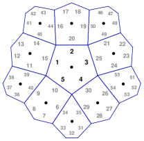
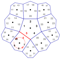
Refer to caption
Refer to caption
Refer to caption
Refer to caption
Refer to caption
Refer to caption
Figure 10: Schematic contraction of 11 pentagons, using contractions over joint edges, self-contractions and cyclic permutations of indices. Contracted edges and indices are marked in red, while cyclic permutations are shown by circular arrows.

After all tensors are contracted, we are left with a boundary of edges whose indices are still clockwise-oriented, provided that our inital labeling of pentagon edges followed the order in which we contracted the respective tensors. We can think of the remaining indices as specifying our boundary sites, and the contracted indices being bulk sites that were “integrated out”. Note that this contraction process is possible for planar graphs for which a Kasteleyn orientation is guaranteed to exist Kasteleyn (1961).

In principle, we have the freedom to cyclically permute the indices of each inital tensor. We can fix this freedom by using symmetry constraints on the generating matrix Ai,jsubscript𝐴𝑖𝑗A_{i,j}. For anti-periodic boundary conditions, we require Ai,jsubscript𝐴𝑖𝑗A_{i,j} to be positive for i>j𝑖𝑗i>j and negative for i<j𝑖𝑗i<j. The condition is retained for the full contracted state if we restrict ourselves to applying cyclic permutations only on the indices of the “inner” tensor from which we contract outwards, and affix the lowest index of each “outer tensor” to the edge over which it is first contracted. These conditions on Ai,jsubscript𝐴𝑖𝑗A_{i,j} allowed us to produce physical covariance matrices with Γi,j>0subscriptΓ𝑖𝑗0\Gamma_{i,j}>0 for i>j𝑖𝑗i>j, as well.

For periodic boundary conditions, Ai,jsubscript𝐴𝑖𝑗A_{i,j} should be positive for |ij|<L/2𝑖𝑗𝐿2|i-j|<L/2 (with number of indices L𝐿L) and negative otherwise. This can be achieved using the same index labeling rules, but choosing only the central tensor’s generating matrix to produce a locally anti-periodic state, while keeping the states corresponding to all other local tensors as periodic.

Periodic boundary conditions are less convenient for numerical studies, as overlap between positive and negative correlations can occur for networks of finite size. For this reason, we have focused on anti-periodic boundary conditions in our work. In the infinite-size limit, of course, both choices of boundary conditions should lead to the same physical properties of the boundary states.

Appendix E Explicit generating matrices and numerical results

E.1 Regular tilings

We start by discussing the correlations achieved for regular tilings. We can produce the boundary theory with 1/dsimilar-toabsent1𝑑\sim 1/d falloff using a regular {3,k}3𝑘\{3,k\} tiling with k6𝑘6k\geq 6. The critical parameter a=acrit𝑎subscript𝑎crita=a_{\text{crit}} for each k𝑘k can be found by maximizing mean long-range correlations (2/L)k=1L/2|Γk,k+L/2|2𝐿superscriptsubscript𝑘1𝐿2subscriptΓ𝑘𝑘𝐿2({2}/{L})\sum_{k=1}^{L/2}|\Gamma_{k,k+L/2}| in the covariance matrix. For k>6𝑘6k>6, the tilings can be embedded into the Poincaré disk with metric

ds2=4dr2+r2dϕ2(1r2)2 ,dsuperscript𝑠24dsuperscript𝑟2superscript𝑟2dsuperscriptitalic-ϕ2superscript1superscript𝑟22 ,\text{d}s^{2}=4\,\frac{\text{d}r^{2}+r^{2}\text{d}\phi^{2}}{(1-r^{2})^{2}}\text{ ,} (86)

using polar coordinates (r,ϕ)𝑟italic-ϕ(r,\phi) with 0r<10𝑟10\leq r<1 and 0ϕ<2π0italic-ϕ2𝜋0\leq\phi<2\pi. As the Poincaré disk represents an infinite volume, we cut off our tilings at a radius r=rc𝑟subscript𝑟𝑐r=r_{c}. For the flat case k=6𝑘6k=6, we simply cut off at Euclidean distance dcsubscript𝑑𝑐d_{c} (with all edges set to unit length). We find the following values of acritsubscript𝑎crita_{\text{crit}} for a given d𝑑d (k=6𝑘6k=6) or rcsubscript𝑟𝑐r_{c} (k>6𝑘6k>6):

       dcsubscript𝑑𝑐d_{c} k=6𝑘6k=6: rcsubscript𝑟𝑐r_{c} k=7𝑘7k=7: k=8𝑘8k=8: k=9𝑘9k=9: k=10𝑘10k=10: k=11𝑘11k=11: k=12𝑘12k=12:
       10 0.5779 0.95 0.6063 0.6213 0.6378 0.6482 0.6529 0.6650
       15 0.5804 0.98 0.6051 0.6203 0.6404 0.6447 0.6618 0.6639
       20 0.5806 0.99 0.6082 0.6244 0.6393 0.6502 0.6575 0.6661

Note that increasing k𝑘k leads to a larger acsubscript𝑎𝑐a_{c}. We argue that this may compensate for the “leaking” of correlations into the higher-curvature bulk. While in principle it is possible to extend this reasoning to positive-curvature (spherical) tilings, the largest triangular tiling {3,5}35\{3,5\} corresponds to an icosahedron with only 20 triangles. Thus, no proper choice of an asymptotic boundary can be made.

E.2 MERA

We now turn to discussing how the MERA framework can be related to our approach. The MERA tensor network consists of two types of tensors, isometries and disentanglers with three and four legs, respectively. Thus, the lattice for the equivalent matchgate tensor consists of triangles and quadrilaterals. In the matchgate setting, the MERA tensors are thus fully specified by a 3×3333\times 3 generating matrix S𝑆S and a 4×4444\times 4 matrix B𝐵B, corresponding to isometries and disentanglers, respectively. For norm-preserving tensors, i.e. unitary disentanglers and isometries, real generating matrices are restricted to the components

A𝐴\displaystyle A =(01+x2cosθ1+x2sinθ1+x2cosθ0x1+x2sinθx0) ,absent01superscript𝑥2𝜃1superscript𝑥2𝜃1superscript𝑥2𝜃0𝑥1superscript𝑥2𝜃𝑥0 ,\displaystyle=\left(\begin{array}[]{ccc}\phantom{-}0&\phantom{-}\sqrt{1+x^{2}}\cos\theta&\phantom{-}\sqrt{1+x^{2}}\sin\theta\\ -\sqrt{1+x^{2}}\cos\theta&\phantom{-}0&\phantom{-}x\\ -\sqrt{1+x^{2}}\sin\theta&-x&\phantom{-}0\end{array}\right)\text{ , } (90)
B𝐵\displaystyle B =(0y1+y2cosϕ1+y2sinϕy01+y2sinϕ1+y2cosϕ1+y2cosϕ1+y2sinϕ0y1+y2sinϕ1+y2cosϕy0) ,absent0𝑦1superscript𝑦2italic-ϕ1superscript𝑦2italic-ϕ𝑦01superscript𝑦2italic-ϕ1superscript𝑦2italic-ϕ1superscript𝑦2italic-ϕ1superscript𝑦2italic-ϕ0𝑦1superscript𝑦2italic-ϕ1superscript𝑦2italic-ϕ𝑦0 ,\displaystyle=\left(\begin{array}[]{cccc}\phantom{-}0&\phantom{-}y&\phantom{-}\sqrt{1+y^{2}}\cos\phi&\phantom{-}\sqrt{1+y^{2}}\sin\phi\\ -y&\phantom{-}0&-\sqrt{1+y^{2}}\sin\phi&\phantom{-}\sqrt{1+y^{2}}\cos\phi\\ -\sqrt{1+y^{2}}\cos\phi&\phantom{-}\sqrt{1+y^{2}}\sin\phi&\phantom{-}0&\phantom{-}y\\ -\sqrt{1+y^{2}}\sin\phi&-\sqrt{1+y^{2}}\cos\phi&-y&\phantom{-}0\end{array}\right)\text{ ,} (95)

with x,y𝑥𝑦x,y\in\mathbb{R} and θ,ϕ[0,2π]𝜃italic-ϕ02𝜋\theta,\phi\in[0,2\pi]. These free parameters of the model can be set by numerically minimizing the ground-state energy of the translation-invariant Ising Hamiltonian (12). However, with these inputs we were unable to find boundary states that are any more translation-invariant than the regular tilings considered earlier. Instead, we consider a more generic “matchgate MERA” (mMERA) with three- and four-leg generating matrices

A=(0aaa0bab0) , B=(0cefc0deed0cfec0) ,𝐴0𝑎𝑎𝑎0𝑏𝑎𝑏0 , 𝐵0𝑐𝑒𝑓𝑐0𝑑𝑒𝑒𝑑0𝑐𝑓𝑒𝑐0 ,\displaystyle A=\left(\begin{array}[]{ccc}\phantom{-}0&\phantom{-}a&\phantom{-}a\\ -a&\phantom{-}0&\phantom{-}b\\ -a&-b&\phantom{-}0\end{array}\right)\text{ , }\;B=\left(\begin{array}[]{cccc}\phantom{-}0&\phantom{-}c&\phantom{-}e&\phantom{-}f\\ -c&\phantom{-}0&\phantom{-}d&\phantom{-}e\\ -e&-d&\phantom{-}0&\phantom{-}c\\ -f&-e&-c&\phantom{-}0\end{array}\right)\text{ ,} (103)

with the parameters a,b,,f𝑎𝑏𝑓a,b,\dots,f\in\mathbb{R}. Now, again minimizing according to (12), we find that numerical solutions obey the symmetries ce𝑐𝑒c\approx e and adf𝑎𝑑𝑓a\approx d\approx f, thus leaving us with three free parameters to optimize. Intriguingly, these symmetries allow us to express the 4-leg “disentanglers” as contractions of a 3-leg tensor with its conjugate, visualized in Fig. 11. While the individual tensors of our model are no longer norm-preserving, we show in the next section that for large networks, norm preservation can still be achieved. Note that while the usual MERA identities for isometries and disentanglers no longer hold, contractions of the mMERA are still efficient, owing to the matchgate setting.

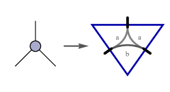
Refer to caption
Refer to caption
Refer to caption
Refer to caption
Figure 11: Top: The standard MERA tensor network (left) in our numerical matchgate setting is equivalent to a network of purely 3-leg tensors (right). Bottom: Isometries, disentanglers, and triangulated disentanglers (from left to right) expressed as matchgate tensors. The free parameters a,b,c𝑎𝑏𝑐a,b,c fix the components of the generating matrices (103).

The central 4-leg tensor of the MERA describes a CFT ground state on four sites, for which the generating matrix A0subscript𝐴0A_{0} and normalization c0subscript𝑐0c_{0} can be given explicitly:

A0=(0a0b0a0a00a0b0b0a00a0a0b0a00) ,c0=11+4a022b02+(2a02b02)2 ,formulae-sequencesubscript𝐴00subscript𝑎0subscript𝑏0subscript𝑎0subscript𝑎00subscript𝑎0subscript𝑏0subscript𝑏0subscript𝑎00subscript𝑎0subscript𝑎0subscript𝑏0subscript𝑎00 ,subscript𝑐0114superscriptsubscript𝑎022superscriptsubscript𝑏02superscript2superscriptsubscript𝑎02superscriptsubscript𝑏022 ,A_{0}=\left(\begin{array}[]{cccc}\phantom{-}0&\phantom{-}a_{0}&\phantom{-}b_{0}&\phantom{-}a_{0}\\ -a_{0}&\phantom{-}0&\phantom{-}a_{0}&\phantom{-}b_{0}\\ -b_{0}&-a_{0}&\phantom{-}0&\phantom{-}a_{0}\\ -a_{0}&-b_{0}&-a_{0}&\phantom{-}0\end{array}\right)\text{ ,}\quad c_{0}=\frac{1}{\sqrt{1+4a_{0}^{2}-2b_{0}^{2}+(2a_{0}^{2}-b_{0}^{2})^{2}}}\text{ ,} (104)

where the constants a0subscript𝑎0a_{0} and b0subscript𝑏0b_{0} are found by analytically minimizing (12), yielding

a0=1+1210.3066 ,b0=68+8a0+532a02616a03290a0458a0543+16a0340a02474a03250a0450a050.2346 .formulae-sequencesubscript𝑎011210.3066 ,subscript𝑏0688subscript𝑎0532superscriptsubscript𝑎02616superscriptsubscript𝑎03290superscriptsubscript𝑎0458superscriptsubscript𝑎054316subscript𝑎0340superscriptsubscript𝑎02474superscriptsubscript𝑎03250superscriptsubscript𝑎0450superscriptsubscript𝑎050.2346 .a_{0}=\sqrt{1+\frac{1}{\sqrt{2}}}-1\approx 0.3066\text{ ,}\quad b_{0}=\frac{68+8a_{0}+532a_{0}^{2}-616a_{0}^{3}-290a_{0}^{4}-58a_{0}^{5}}{43+16a_{0}-340a_{0}^{2}-474a_{0}^{3}-250a_{0}^{4}-50a_{0}^{5}}\approx 0.2346\text{ .} (105)

All remaining tensors are numerically optimized within our three-parameter model. As shown in Fig. 12, the minimal energy density ϵ=H/Litalic-ϵdelimited-⟨⟩𝐻𝐿\epsilon=\langle H\rangle/L converges quadratically with the number of boundary sites L𝐿L. The optimal values for a,b,c𝑎𝑏𝑐a,b,c converge as well. At L=1024𝐿1024L=1024, those are given by a=0.6854𝑎0.6854a=0.6854, b=0.5246𝑏0.5246b=0.5246, and c=0.2172𝑐0.2172c=0.2172, yielding a ground-state energy density ϵ0=0.636533subscriptitalic-ϵ00.636533\epsilon_{0}=-0.636533 (decimals given up to convergent digits). The relative error with respect to the continuum solution ϵ0=2/πsubscriptitalic-ϵ02𝜋\epsilon_{0}=2/\pi is about 0.014%percent0.0140.014\%. Note that this MERA model only has bond dimension χ=2𝜒2\chi=2, and that increasing χ𝜒\chi would increase the size of the generating matrices and the number of free parameters, presumably allowing for even higher accuracy.
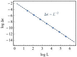
Refer to caption
Figure 12: Energy density ϵitalic-ϵ\epsilon of the MERA boundary state of L𝐿L sites, minimized with respect to the Ising Hamiltonian (12). Plotted are the differences Δϵ=ϵ(2L)ϵ(L)Δitalic-ϵitalic-ϵ2𝐿italic-ϵ𝐿\Delta\epsilon=\epsilon(2L)-\epsilon(L) between two MERA layers, with a quadratic falloff, fitted from the data, shown as a gray line.

E.3 Conformal data

In this subsection, we show how to obtain conformal data from the approach taken here. The Ising theory at criticality can be described by a 1+1-dimensional conformal field theory (CFT) Francesco et al. (1997). The operator content of this theory is defined by its primary fields, whose scaling behavior is exactly known. This is because two-dimensional CFTs can be solved exactly, usually by mapping the space and time coordinates (x,t)𝑥𝑡(x,t) to a complex number z=x+it𝑧𝑥i𝑡z=x+\,\mathrm{i}\,t and its complex conjugate z¯=xit¯𝑧𝑥i𝑡\bar{z}=x-\,\mathrm{i}\,t. (Quasi-) primary fields ϕ(z)italic-ϕ𝑧\phi(z) have associated conformal weights hϕsubscriptitalic-ϕh_{\phi} and h¯ϕsubscript¯italic-ϕ\bar{h}_{\phi}, with correlations between different space-time points z𝑧z and w𝑤w being given by

ϕ(z)ϕ(w)=Cϕ,ϕ(zw)2hϕ(z¯w¯)2h¯ϕ .delimited-⟨⟩italic-ϕ𝑧italic-ϕ𝑤subscript𝐶italic-ϕitalic-ϕsuperscript𝑧𝑤2subscriptitalic-ϕsuperscript¯𝑧¯𝑤2subscript¯italic-ϕ .\langle\phi(z)\phi(w)\rangle=\frac{C_{\phi,\phi}}{(z-w)^{2h_{\phi}}(\bar{z}-\bar{w})^{2\bar{h}_{\phi}}}\text{ .} (106)

The constant Cϕ,ϕsubscript𝐶italic-ϕitalic-ϕC_{\phi,\phi} is not a fundamental CFT parameter, but determined by the normalization of ϕitalic-ϕ\phi. As we are restricting ourselves to correlations on time-slices, we will find correlators of the form

ϕ(x)ϕ(y)=Cϕ,ϕ|xy|2(hϕ+h¯ϕ)=Cϕ,ϕ|xy|2Δϕ ,delimited-⟨⟩italic-ϕ𝑥italic-ϕ𝑦subscript𝐶italic-ϕitalic-ϕsuperscript𝑥𝑦2subscriptitalic-ϕsubscript¯italic-ϕsubscript𝐶italic-ϕitalic-ϕsuperscript𝑥𝑦2subscriptΔitalic-ϕ ,\langle\phi(x)\phi(y)\rangle=\frac{C_{\phi,\phi}}{|x-y|^{2(h_{\phi}+\bar{h}_{\phi})}}=\frac{C_{\phi,\phi}}{|x-y|^{2\Delta_{\phi}}}\text{ ,} (107)

expressed in terms of the scaling dimension Δϕ=hϕ+h¯ϕsubscriptΔitalic-ϕsubscriptitalic-ϕsubscript¯italic-ϕ\Delta_{\phi}=h_{\phi}+\bar{h}_{\phi}. The three-point functions of primary fields ϕ,χitalic-ϕ𝜒\phi,\chi and ω𝜔\omega have the form

ϕ(x)χ(y)ω(z)=Cϕ,ϕCχ,χCω,ωCϕ,χ,ω|xy|Δϕ+ΔχΔω|yz|Δχ+ΔωΔϕ|zx|Δω+ΔϕΔχ ,delimited-⟨⟩italic-ϕ𝑥𝜒𝑦𝜔𝑧subscript𝐶italic-ϕitalic-ϕsubscript𝐶𝜒𝜒subscript𝐶𝜔𝜔subscript𝐶italic-ϕ𝜒𝜔superscript𝑥𝑦subscriptΔitalic-ϕsubscriptΔ𝜒subscriptΔ𝜔superscript𝑦𝑧subscriptΔ𝜒subscriptΔ𝜔subscriptΔitalic-ϕsuperscript𝑧𝑥subscriptΔ𝜔subscriptΔitalic-ϕsubscriptΔ𝜒 ,\langle\phi(x)\chi(y)\omega(z)\rangle=\frac{\sqrt{C_{\phi,\phi}C_{\chi,\chi}C_{\omega,\omega}}\;C_{\phi,\chi,\omega}}{|x-y|^{\Delta_{\phi}+\Delta_{\chi}-\Delta_{\omega}}\;|y-z|^{\Delta_{\chi}+\Delta_{\omega}-\Delta_{\phi}}\;|z-x|^{\Delta_{\omega}+\Delta_{\phi}-\Delta_{\chi}}}\text{ ,} (108)

with the structure constants Cϕ,χ,ωsubscript𝐶italic-ϕ𝜒𝜔C_{\phi,\chi,\omega} being fundamental CFT quantities.

For the Ising CFT in two dimensions, there are three primary fields: The identity 𝟙1\mathds{1}, the energy density ϵitalic-ϵ\epsilon and the spin (or “order parameter”) σ𝜎\sigma. The Jordan-Wigner transformation gives us an alternative description in terms of the fermionic fields ψ𝜓\psi and ψ¯¯𝜓\bar{\psi}. The corresponding scaling dimensions are the following.

       Field ϕitalic-ϕ\phi 𝟙1\mathds{1} ϵitalic-ϵ\epsilon σ𝜎\sigma ψ𝜓\psi ψ¯¯𝜓\bar{\psi}
       hϕsubscriptitalic-ϕh_{\phi} 0 1/2 1/16 1/2 0
       h¯ϕsubscript¯italic-ϕ\bar{h}_{\phi} 0 1/2 1/16 0 1/2
       ΔϕsubscriptΔitalic-ϕ\Delta_{\phi} 0 1 1/8 1/2 1/2

Furthermore, the structure constants in the spin sector are Cσ,σ,𝟙=1subscript𝐶𝜎𝜎11C_{\sigma,\sigma,\mathds{1}}=1 and Cσ,σ,ϵ=12subscript𝐶𝜎𝜎italic-ϵ12C_{\sigma,\sigma,\epsilon}=\frac{1}{2}.

For the Gaussian states produced by our matchgate tensor networks, all the information on correlators is stored in the Majorana covariance matrix with entries Γj,k=i2[γj,γk]subscriptΓ𝑗𝑘delimited-⟨⟩i2subscript𝛾𝑗subscript𝛾𝑘\Gamma_{j,k}=\langle\tfrac{\,\mathrm{i}\,}{2}[\operatorname{\gamma}_{j},\operatorname{\gamma}_{k}]\rangle. Before calculating the scaling dimensions, let us first prove a useful identity regarding the covariance matrix of odd-pairing Hamiltonians of the form

HOP=ik,dJk,dγkγk+2d1 ,subscript𝐻OPisubscript𝑘𝑑subscript𝐽𝑘𝑑subscript𝛾𝑘subscript𝛾𝑘2𝑑1 ,H_{\text{OP}}=\,\mathrm{i}\,\sum_{k,d}J_{k,d}\,\operatorname{\gamma}_{k}\operatorname{\gamma}_{k+2d-1}\text{ ,} (109)

with the couplings Jk,dsubscript𝐽𝑘𝑑J_{k,d}\in\mathbb{R} between Majorana sites at odd distance. In particular, this includes Hamiltonians with only nearest-neighbor Majorana coupling with Jk,d=δd,1Jksubscript𝐽𝑘𝑑subscript𝛿𝑑1subscript𝐽𝑘J_{k,d}=\delta_{d,1}\,J_{k}, such as the Ising model considered above.

Lemma 8 (Covariance matrices of odd-pairing Majorana Hamiltonians).

Eigenstates of Hamiltonians HOPsubscript𝐻OPH_{\text{OP}} of the form (109) are described by a covariance matrix ΓΓ\Gamma whose entries Γj,ksubscriptΓ𝑗𝑘\Gamma_{j,k} vanish for even j+k𝑗𝑘j\,{+}\,k.

Proof.

Consider an eigenstate |ψ=x{0,1}n𝒯(x)|xket𝜓subscript𝑥superscript01𝑛𝒯𝑥ket𝑥\left.\left|{\psi}\right.\right\rangle=\sum_{x\in\{0,1\}^{n}}\mathcal{T}(x)\left.\left|{x}\right.\right\rangle of HOPsubscript𝐻OPH_{\text{OP}} with eigenenergy E𝐸E. We will first prove that 𝒯(x)𝒯𝑥\mathcal{T}(x)\in\mathbb{R} for all x{0,1}n𝑥superscript01𝑛x\in\{0,1\}^{n}. We first note that we can write

HOPsubscript𝐻OP\displaystyle H_{\text{OP}} =ii,d(J2i1,dγ2i1γ2i+2d2+J2i,dγ2iγ2i+2d1)absentisubscript𝑖𝑑subscript𝐽2𝑖1𝑑subscript𝛾2𝑖1subscript𝛾2𝑖2𝑑2subscript𝐽2𝑖𝑑subscript𝛾2𝑖subscript𝛾2𝑖2𝑑1\displaystyle=\,\mathrm{i}\,\sum_{i,d}\left(J_{2i-1,d}\,\operatorname{\gamma}_{2i-1}\operatorname{\gamma}_{2i+2d-2}+J_{2i,d}\,\operatorname{\gamma}_{2i}\operatorname{\gamma}_{2i+2d-1}\right)
=i,d(J2i1,d(fi+fi)(fi+d1fi+d1)+J2i,d(fifi)(fi+d+fi+d)) ,absentsubscript𝑖𝑑subscript𝐽2𝑖1𝑑subscriptsuperscriptfabsent𝑖subscriptsuperscriptf𝑖subscriptsuperscriptfabsent𝑖𝑑1subscriptsuperscriptf𝑖𝑑1subscript𝐽2𝑖𝑑subscriptsuperscriptfabsent𝑖subscriptsuperscriptf𝑖subscriptsuperscriptfabsent𝑖𝑑subscriptsuperscriptf𝑖𝑑 ,\displaystyle=\sum_{i,d}\left(J_{2i-1,d}(\operatorname{f}^{\phantom{\dagger}}_{i}+\operatorname{f}^{\dagger}_{i})(\operatorname{f}^{\phantom{\dagger}}_{i+d-1}-\operatorname{f}^{\dagger}_{i+d-1})+J_{2i,d}(\operatorname{f}^{\phantom{\dagger}}_{i}-\operatorname{f}^{\dagger}_{i})(\operatorname{f}^{\phantom{\dagger}}_{i+d}+\operatorname{f}^{\dagger}_{i+d})\right)\text{ ,} (110)

which implies that the Hamiltonian is not only Hermitian but also invariant under complex conjugation HOP=HOPsuperscriptsubscript𝐻OPsubscript𝐻OPH_{\text{OP}}^{*}=H_{\text{OP}}. We now decompose our eigenstate into its real and imaginary part denoted by |ψ=[|ψ]+i[|ψ]ket𝜓ket𝜓iket𝜓\left.\left|{\psi}\right.\right\rangle=\Re[\left.\left|{\psi}\right.\right\rangle]+\,\mathrm{i}\,\Im[\left.\left|{\psi}\right.\right\rangle]. The eigenequation reads

HOP|ψ=E|ψsubscript𝐻OPket𝜓𝐸ket𝜓\displaystyle H_{\text{OP}}\left.\left|{\psi}\right.\right\rangle=E\left.\left|{\psi}\right.\right\rangle (111)

and its complex conjugate can be expressed as

(HOP|ψ)=HOP|ψ=HOP[|ψ]iHOP[|ψ]=!E[|ψ]iE[|ψ]superscriptsubscript𝐻OPket𝜓subscript𝐻OPsuperscriptket𝜓subscript𝐻OPket𝜓isubscript𝐻OPket𝜓𝐸ket𝜓i𝐸ket𝜓\displaystyle(H_{\text{OP}}\left.\left|{\psi}\right.\right\rangle)^{*}=H_{\text{OP}}\left.\left|{\psi}\right.\right\rangle^{*}=H_{\text{OP}}\,\Re[\left.\left|{\psi}\right.\right\rangle]-\,\mathrm{i}\,H_{\text{OP}}\,\Im[\left.\left|{\psi}\right.\right\rangle]\overset{!}{=}E\,\Re[\left.\left|{\psi}\right.\right\rangle]-\,\mathrm{i}\,E\,\Im[\left.\left|{\psi}\right.\right\rangle] (112)

where the only difference to the original equation is the minus sign. Adding and subtracting these two equations yields

HOP[|ψ]=E[|ψ]subscript𝐻OPket𝜓𝐸ket𝜓\displaystyle H_{\text{OP}}\,\Re[\left.\left|{\psi}\right.\right\rangle]=E\,\Re[\left.\left|{\psi}\right.\right\rangle] (113)

and

HOP[|ψ]=E[|ψ]subscript𝐻OPket𝜓𝐸ket𝜓\displaystyle H_{\text{OP}}\,\Im[\left.\left|{\psi}\right.\right\rangle]=E\,\Im[\left.\left|{\psi}\right.\right\rangle] (114)

which means that [|ψ]ket𝜓\Re[\left.\left|{\psi}\right.\right\rangle] and [|ψ]ket𝜓\Im[\left.\left|{\psi}\right.\right\rangle] are both eigenvectors. If the spectrum is non-degenerate then they are collinear and hence we can assume that |ψ=|ψsuperscriptket𝜓ket𝜓\left.\left|{\psi}\right.\right\rangle^{*}=\left.\left|{\psi}\right.\right\rangle up to a phase. If the spectrum is degenerate then we can also choose real eigenstates because span(|ψ,|ψ)=span([|ψ],[|ψ])spanket𝜓superscriptket𝜓spanket𝜓ket𝜓\text{span}(\left.\left|{\psi}\right.\right\rangle,\left.\left|{\psi}\right.\right\rangle^{*})=\text{span}(\Re[\left.\left|{\psi}\right.\right\rangle],\Im[\left.\left|{\psi}\right.\right\rangle]). In the context of matchgates, this means that all eigenstates are expressed by real generating matrices, which are therefore a suitable ansatz for ground states of such Hamiltonians.

Next, we show that the matrix elements of the covariance matrix vanish for even j+k𝑗𝑘j\,{+}\,k. For j=k𝑗𝑘j\,{=}\,k this is true by definition, so we assume jk𝑗𝑘j\,{\neq}\,k. For even j𝑗j and k𝑘k we find i2[γj,γk]=iγjγk=i(fj/2fj/2)(fk/2fk/2)i2subscript𝛾𝑗subscript𝛾𝑘isubscript𝛾𝑗subscript𝛾𝑘isubscriptsuperscriptfabsent𝑗2subscriptsuperscriptf𝑗2subscriptsuperscriptfabsent𝑘2subscriptsuperscriptf𝑘2\frac{\,\mathrm{i}\,}{2}[\operatorname{\gamma}_{j},\operatorname{\gamma}_{k}]=\,\mathrm{i}\,\operatorname{\gamma}_{j}\operatorname{\gamma}_{k}=-\,\mathrm{i}\,(\operatorname{f}^{\phantom{\dagger}}_{j/2}-\operatorname{f}^{\dagger}_{j/2})(\operatorname{f}^{\phantom{\dagger}}_{k/2}-\operatorname{f}^{\dagger}_{k/2}) while for odd j𝑗j and k𝑘k we have i2[γj,γk]=iγjγk=i(f(j+1)/2+f(j+1)/2)(f(k+1)/2+f(k+1)/2)i2subscript𝛾𝑗subscript𝛾𝑘isubscript𝛾𝑗subscript𝛾𝑘isubscriptsuperscriptfabsent𝑗12subscriptsuperscriptf𝑗12subscriptsuperscriptfabsent𝑘12subscriptsuperscriptf𝑘12\frac{\,\mathrm{i}\,}{2}[\operatorname{\gamma}_{j},\operatorname{\gamma}_{k}]=\,\mathrm{i}\,\operatorname{\gamma}_{j}\operatorname{\gamma}_{k}=\,\mathrm{i}\,(\operatorname{f}^{\phantom{\dagger}}_{(j+1)/2}+\operatorname{f}^{\dagger}_{(j+1)/2})(\operatorname{f}^{\phantom{\dagger}}_{(k+1)/2}+\operatorname{f}^{\dagger}_{(k+1)/2}). Either way, these Hermitian operators have purely imaginary coefficients in terms of creation and annihilation operators. Evaluated in a state with real amplitudes, as shown above, the expectation value can only be imaginary. As all observables are real, it must therefore vanish altogether. ∎

Now let us relate the covariance matrix entries Γj,ksubscriptΓ𝑗𝑘\Gamma_{j,k} to the primary fields. By construction of our covariance matrix in Section C, ψ|ψ=1inner-product𝜓𝜓1\left\langle\psi\middle|\psi\right\rangle=1 and thus the identity 𝟙1\mathds{1} does not scale. However, the normalization factor Z𝑍Z in (51) can in principle scale with the size of the contracted network. To ensure normalization, we have to act on each of the NTsubscript𝑁𝑇N_{T} contracted tensors with a scaling factor f=Z1/(2NT)𝑓superscript𝑍12subscript𝑁𝑇f=Z^{-1/(2N_{T})}. We find that this factor f𝑓f converges for large systems, ensuring Δ𝟙=0subscriptΔ10\Delta_{\mathds{1}}=0. Explicitly, f{3,6}0.972subscript𝑓360.972f_{\{3,6\}}\approx 0.972 and f{3,7}0.941subscript𝑓370.941f_{\{3,7\}}\approx 0.941 for the regular tilings and fmMERA0.959subscript𝑓mMERA0.959f_{\text{mMERA}}\approx 0.959 for the mMERA.

We identify the fermionic fields ψ𝜓\psi and ψ¯¯𝜓\bar{\psi} with physical operators ψk:=fk=12(γ2k1+iγ2k)assignsubscript𝜓𝑘subscriptsuperscriptfabsent𝑘12subscript𝛾2𝑘1isubscript𝛾2𝑘\psi_{k}:=\operatorname{f}^{\phantom{\dagger}}_{k}=\frac{1}{2}(\operatorname{\gamma}_{2k-1}+\,\mathrm{i}\,\operatorname{\gamma}_{2k}) and ψ¯k:=ifk=12(iγ2k1+γ2k)assignsubscript¯𝜓𝑘isubscriptsuperscriptf𝑘12isubscript𝛾2𝑘1subscript𝛾2𝑘\bar{\psi}_{k}:=\,\mathrm{i}\,\operatorname{f}^{\dagger}_{k}=\frac{1}{2}(\,\mathrm{i}\,\operatorname{\gamma}_{2k-1}+\operatorname{\gamma}_{2k}). We then find that

ψjψk=ψ¯jψ¯k=14(Γ2j,2k1+Γ2j1,2k) .delimited-⟨⟩subscript𝜓𝑗subscript𝜓𝑘delimited-⟨⟩subscript¯𝜓𝑗subscript¯𝜓𝑘14subscriptΓ2𝑗2𝑘1subscriptΓ2𝑗12𝑘 .\langle\psi_{j}\psi_{k}\rangle=\langle\bar{\psi}_{j}\bar{\psi}_{k}\rangle=\frac{1}{4}\left(\Gamma_{2j,2k-1}+\Gamma_{2j-1,2k}\right)\text{ .} (115)

Note that we have used Lemma 8 to simplify the result. As we are considering Gaussian states, ψk=ψ¯k=0delimited-⟨⟩subscript𝜓𝑘delimited-⟨⟩subscript¯𝜓𝑘0\langle\psi_{k}\rangle=\langle\bar{\psi}_{k}\rangle=0 for any k𝑘k, so we do not have to consider expectation values of the individual fields. Next, we compute the energy density ϵitalic-ϵ\epsilon. On site k𝑘k, we simply consider the local operator ϵk:=iψkψ¯k=i2γ2k1γ2kassignsubscriptitalic-ϵ𝑘isubscript𝜓𝑘subscript¯𝜓𝑘i2subscript𝛾2𝑘1subscript𝛾2𝑘\epsilon_{k}:=\,\mathrm{i}\,\psi_{k}\bar{\psi}_{k}=\frac{\,\mathrm{i}\,}{2}\operatorname{\gamma}_{2k-1}\operatorname{\gamma}_{2k}. Using Wick’s theorem, the two-point functions follow as 111With our definition, ϵ0delimited-⟨⟩italic-ϵ0\langle\epsilon\rangle\neq 0, so we need to subtract the field’s expectation value, equivalent to using a field ϵ=ϵϵsuperscriptitalic-ϵitalic-ϵdelimited-⟨⟩italic-ϵ\epsilon^{\prime}=\epsilon-\langle\epsilon\rangle.

ϵjϵkϵjϵk=14(γ2j1γ2jγ2k1γ2k+γ2j1γ2jγ2k1γ2k)=14Γ2j1,2kΓ2j,2k1 .delimited-⟨⟩subscriptitalic-ϵ𝑗subscriptitalic-ϵ𝑘delimited-⟨⟩subscriptitalic-ϵ𝑗delimited-⟨⟩subscriptitalic-ϵ𝑘14delimited-⟨⟩subscript𝛾2𝑗1subscript𝛾2𝑗subscript𝛾2𝑘1subscript𝛾2𝑘delimited-⟨⟩subscript𝛾2𝑗1subscript𝛾2𝑗delimited-⟨⟩subscript𝛾2𝑘1subscript𝛾2𝑘14subscriptΓ2𝑗12𝑘subscriptΓ2𝑗2𝑘1 .\langle\epsilon_{j}\epsilon_{k}\rangle-\langle\epsilon_{j}\rangle\langle\epsilon_{k}\rangle=\frac{1}{4}\left(-\langle\operatorname{\gamma}_{2j-1}\operatorname{\gamma}_{2j}\operatorname{\gamma}_{2k-1}\operatorname{\gamma}_{2k}\rangle+\langle\operatorname{\gamma}_{2j-1}\operatorname{\gamma}_{2j}\rangle\langle\operatorname{\gamma}_{2k-1}\operatorname{\gamma}_{2k}\rangle\right)=\frac{1}{4}\Gamma_{2j-1,2k}\Gamma_{2j,2k-1}\text{ .} (116)

The order σ𝜎\sigma is a nonlocal operator in the Majorana picture but corresponds to a σxsuperscript𝜎𝑥\sigma^{x} operator222In fact, ϵitalic-ϵ\epsilon can be related to the σzsuperscript𝜎𝑧\sigma^{z} operator, which conveniently acts locally in terms of Majorana operators, as well. in the spin picture, obtained through a Jordan-Wigner transformation. A two-point correlator of σkxsubscriptsuperscript𝜎𝑥𝑘\sigma^{x}_{k} at different sites k𝑘k corresponds to a chain of Majorana operators,

σkxσk+1xdelimited-⟨⟩subscriptsuperscript𝜎𝑥𝑘subscriptsuperscript𝜎𝑥𝑘1\displaystyle\langle\sigma^{x}_{k}\sigma^{x}_{k+1}\rangle =iγ2kγ2k+1=Pf(Γ2k,2kΓ2k,2k+1Γ2k+1,2kΓ2k+1,2k+1) ,absentidelimited-⟨⟩subscript𝛾2𝑘subscript𝛾2𝑘1PfsubscriptΓ2𝑘2𝑘subscriptΓ2𝑘2𝑘1subscriptΓ2𝑘12𝑘subscriptΓ2𝑘12𝑘1 ,\displaystyle=-\,\mathrm{i}\,\langle\operatorname{\gamma}_{2k}\operatorname{\gamma}_{2k+1}\rangle=-\mathrm{Pf}\left(\begin{array}[]{ll}\Gamma_{2k,2k}&\Gamma_{2k,2k+1}\\ \Gamma_{2k+1,2k}&\Gamma_{2k+1,2k+1}\end{array}\right)\text{ ,} (119)
σkxσk+2xdelimited-⟨⟩subscriptsuperscript𝜎𝑥𝑘subscriptsuperscript𝜎𝑥𝑘2\displaystyle\langle\sigma^{x}_{k}\sigma^{x}_{k+2}\rangle =γ2kγ2k+1γ2k+2γ2k+3=Pf(Γ2k,2kΓ2k,2k+1Γ2k,2k+2Γ2k,2k+3Γ2k+1,2kΓ2k+1,2k+1Γ2k+1,2k+2Γ2k+1,2k+3Γ2k+2,2kΓ2k+2,2k+1Γ2k+2,2k+2Γ2k+2,2k+3Γ2k+3,2kΓ2k+3,2k+1Γ2k+3,2k+2Γ2k+3,2k+3) ,absentdelimited-⟨⟩subscript𝛾2𝑘subscript𝛾2𝑘1subscript𝛾2𝑘2subscript𝛾2𝑘3PfsubscriptΓ2𝑘2𝑘subscriptΓ2𝑘2𝑘1subscriptΓ2𝑘2𝑘2subscriptΓ2𝑘2𝑘3subscriptΓ2𝑘12𝑘subscriptΓ2𝑘12𝑘1subscriptΓ2𝑘12𝑘2subscriptΓ2𝑘12𝑘3subscriptΓ2𝑘22𝑘subscriptΓ2𝑘22𝑘1subscriptΓ2𝑘22𝑘2subscriptΓ2𝑘22𝑘3subscriptΓ2𝑘32𝑘subscriptΓ2𝑘32𝑘1subscriptΓ2𝑘32𝑘2subscriptΓ2𝑘32𝑘3 ,\displaystyle=-\langle\,\operatorname{\gamma}_{2k}\operatorname{\gamma}_{2k+1}\operatorname{\gamma}_{2k+2}\operatorname{\gamma}_{2k+3}\rangle=\mathrm{Pf}\left(\begin{array}[]{llll}\Gamma_{2k,2k}&\Gamma_{2k,2k+1}&\Gamma_{2k,2k+2}&\Gamma_{2k,2k+3}\\ \Gamma_{2k+1,2k}&\Gamma_{2k+1,2k+1}&\Gamma_{2k+1,2k+2}&\Gamma_{2k+1,2k+3}\\ \Gamma_{2k+2,2k}&\Gamma_{2k+2,2k+1}&\Gamma_{2k+2,2k+2}&\Gamma_{2k+2,2k+3}\\ \Gamma_{2k+3,2k}&\Gamma_{2k+3,2k+1}&\Gamma_{2k+3,2k+2}&\Gamma_{2k+3,2k+3}\\ \end{array}\right)\text{ ,} (124)
σjxσkxdelimited-⟨⟩subscriptsuperscript𝜎𝑥𝑗subscriptsuperscript𝜎𝑥𝑘\displaystyle\langle\sigma^{x}_{j}\sigma^{x}_{k}\rangle =(i)kjγ2jγ2j+1γ2k2γ2k1=(1)kjPf(Γ|[2j,2k1]) .\displaystyle=(-\,\mathrm{i})^{k-j}\,\langle\operatorname{\gamma}_{2j}\operatorname{\gamma}_{2j+1}\dots\operatorname{\gamma}_{2k-2}\operatorname{\gamma}_{2k-1}\rangle=(-1)^{k-j}\,\mathrm{Pf}\left(\Gamma_{|[2j,2k-1]}\right)\text{ .} (125)

The absolute value of the Pfaffian is given by |Pf(M)|=detMPf𝑀𝑀|\mathrm{Pf}\left(M\right)|=\sqrt{\det{M}}. Note that because σkxsubscriptsuperscript𝜎𝑥𝑘\sigma^{x}_{k} is an odd product of Majorana operators, σkx=0delimited-⟨⟩subscriptsuperscript𝜎𝑥𝑘0\langle\sigma^{x}_{k}\rangle=0.

Additionally, we compute the structure constant Cσ,σ,ϵsubscript𝐶𝜎𝜎italic-ϵC_{\sigma,\sigma,\epsilon} from the corresponding three-point correlator:

σjxσkxϵlσjxσkxϵldelimited-⟨⟩subscriptsuperscript𝜎𝑥𝑗subscriptsuperscript𝜎𝑥𝑘subscriptitalic-ϵ𝑙delimited-⟨⟩subscriptsuperscript𝜎𝑥𝑗subscriptsuperscript𝜎𝑥𝑘delimited-⟨⟩subscriptitalic-ϵ𝑙\displaystyle\langle\sigma^{x}_{j}\sigma^{x}_{k}\epsilon_{l}\rangle-\langle\sigma^{x}_{j}\sigma^{x}_{k}\rangle\langle\epsilon_{l}\rangle =12((i)kj+1γ2jγ2j+1γ2k2γ2k1γ2l1γ2l+(1)kjPf(Γ|[2j,2k1])Γ2l1,2l)\displaystyle=\frac{-1}{2}\left((-\,\mathrm{i})^{k-j+1}\langle\operatorname{\gamma}_{2j}\operatorname{\gamma}_{2j+1}\dots\operatorname{\gamma}_{2k-2}\operatorname{\gamma}_{2k-1}\operatorname{\gamma}_{2l-1}\operatorname{\gamma}_{2l}\rangle+(-1)^{k-j}\,\mathrm{Pf}\left(\Gamma_{|[2j,2k-1]}\right)\Gamma_{2l-1,2l}\right) (126)
=(1)kj2(Pf(Γ|[2j,2k1]{2l1,2l})Pf(Γ|[2j,2k1])Γ2l1,2l) .\displaystyle=\frac{(-1)^{k-j}}{2}\left(\mathrm{Pf}\left(\Gamma_{|[2j,2k-1]\cap\{2l-1,2l\}}\right)-\mathrm{Pf}\left(\Gamma_{|[2j,2k-1]}\right)\Gamma_{2l-1,2l}\right)\text{ .} (127)

In order to use this result to compute the value of Cσ,σ,ϵsubscript𝐶𝜎𝜎italic-ϵC_{\sigma,\sigma,\epsilon} as in (108), we consider the special case kj=lk=d𝑘𝑗𝑙𝑘𝑑k-j=l-k=d, for some integer distance d𝑑d. We then expect a scaling

σjxσj+dxϵj+2dσjxσj+dxϵj+2d=Cσ,σCϵ,ϵCσ,σ,ϵ2Δϵd 2Δσ+Δϵ .delimited-⟨⟩subscriptsuperscript𝜎𝑥𝑗subscriptsuperscript𝜎𝑥𝑗𝑑subscriptitalic-ϵ𝑗2𝑑delimited-⟨⟩subscriptsuperscript𝜎𝑥𝑗subscriptsuperscript𝜎𝑥𝑗𝑑delimited-⟨⟩subscriptitalic-ϵ𝑗2𝑑subscript𝐶𝜎𝜎subscript𝐶italic-ϵitalic-ϵsubscript𝐶𝜎𝜎italic-ϵsuperscript2subscriptΔitalic-ϵsuperscript𝑑2subscriptΔ𝜎subscriptΔitalic-ϵ .\langle\sigma^{x}_{j}\sigma^{x}_{j+d}\epsilon_{j+2d}\rangle-\langle\sigma^{x}_{j}\sigma^{x}_{j+d}\rangle\langle\epsilon_{j+2d}\rangle=\frac{C_{\sigma,\sigma}\sqrt{C_{\epsilon,\epsilon}}\;C_{\sigma,\sigma,\epsilon}}{2^{\Delta_{\epsilon}}d^{\,2\Delta_{\sigma}+\Delta_{\epsilon}}}\text{ .} (128)

Using these tools for extracting two- and three-point correlators, we compute the scaling powers pϕsubscript𝑝italic-ϕp_{\phi} for the various fields ϕitalic-ϕ\phi by fitting the dependence of ϕiϕi+ddelimited-⟨⟩subscriptitalic-ϕ𝑖subscriptitalic-ϕ𝑖𝑑\langle\phi_{i}\phi_{i+d}\rangle on distance d𝑑d. The resulting graphs for ϕ{ψ,ϵ,σ}italic-ϕ𝜓italic-ϵ𝜎\phi\in\{\psi,\epsilon,\sigma\} are presented for the regular {3,6}36\{3,6\} and {3,7}37\{3,7\} tilings as well as for the mMERA tiling in figures 13, 14 and 15, respectively. We also compute Cσ,σ,ϵsubscript𝐶𝜎𝜎italic-ϵC_{\sigma,\sigma,\epsilon} with (126) and (128), using the scaling dimensions Δσ,ΔϵsubscriptΔ𝜎subscriptΔitalic-ϵ\Delta_{\sigma},\Delta_{\epsilon} and normalizations Cσ,σ,Cϵ,ϵsubscript𝐶𝜎𝜎subscript𝐶italic-ϵitalic-ϵC_{\sigma,\sigma},C_{\epsilon,\epsilon} from the previous fits as inputs. Furthermore, we compute the energy density ϵ0=H/Lsubscriptitalic-ϵ0delimited-⟨⟩𝐻𝐿\epsilon_{0}=\langle H\rangle/L with respect to the Ising Hamiltonian (12). Note that the regular {3,6}36\{3,6\} and {3,7}37\{3,7\} tilings are not translation invariant, leading to irregularities on small scales and amplified finite-size effects. This also leads to larger deviations from the exact ground state energy density ϵ0=2/πsubscriptitalic-ϵ02𝜋\epsilon_{0}=-2/\pi.

Finally, we can compute the central charge c𝑐c characterizing the CFT. This is achieved by considering the scaling of the entanglement entropy SAsubscript𝑆𝐴S_{A} with the subsystem size =|A|𝐴\ell=|A|. We expect the exact result (11) for a critical theory, with c=1/2𝑐12c=1/2 for an Ising CFT. For a subsystem A=[k,k+]𝐴𝑘𝑘A=[k,k+\ell], SAsubscript𝑆𝐴S_{A} can be computed from the symplectic eigenvalue spectrum of the partial covariance matrix Γ|A\Gamma_{|A} Serafini et al. (2004). In detail, one performs an orthogonal transformation Γ|A=QΓ~|AQT\Gamma_{|A}=Q\,\tilde{\Gamma}_{|A}\,Q^{T} into the form

Γ~|A=i=1L(0λiλi0) ,\tilde{\Gamma}_{|A}=\bigoplus_{i=1}^{L}\left(\begin{matrix}0&\lambda_{i}\\ -\lambda_{i}&0\end{matrix}\right)\text{ ,} (129)

which is most conveniently achieved using numerical Schur decomposition, and then reading off the entanglement entropy as

SA=i=1L(1+λi2log1+λi21λi2log1λi2) .subscript𝑆𝐴superscriptsubscript𝑖1𝐿1subscript𝜆𝑖21subscript𝜆𝑖21subscript𝜆𝑖21subscript𝜆𝑖2 .S_{A}=\sum_{i=1}^{L}\left(-\frac{1+\lambda_{i}}{2}\log\frac{1+\lambda_{i}}{2}-\frac{1-\lambda_{i}}{2}\log\frac{1-\lambda_{i}}{2}\right)\text{ .} (130)

Our combined results for scaling dimensions, the structure constant Cσ,σ,ϵsubscript𝐶𝜎𝜎italic-ϵC_{\sigma,\sigma,\epsilon}, the ground state energy ϵ0subscriptitalic-ϵ0\epsilon_{0} and the central charge c𝑐c are summarized in Table 1 of the main text.
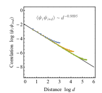
Refer to caption
Refer to caption
Refer to caption
Figure 13: Scaling of primary operators ψ𝜓\psi, ϵitalic-ϵ\epsilon and σ𝜎\sigma in the regular {3,6}36\{3,6\} tiling for boundary states of 84, 282, and 870 Majorana sites (blue, yellow and green points, respectively). Numerical fit of scaling power law shown as grey line. Correlators ϕiϕi+ddelimited-⟨⟩subscriptitalic-ϕ𝑖subscriptitalic-ϕ𝑖𝑑\langle\phi_{i}\phi_{i+d}\rangle of fields ϕitalic-ϕ\phi at distance d𝑑d are averaged over all sites i𝑖i.
Refer to caption
Refer to caption
Refer to caption
Figure 14: Scaling of primary operators ψ𝜓\psi, ϵitalic-ϵ\epsilon and σ𝜎\sigma in the regular {3,7}37\{3,7\} tiling for boundary states of 90, 360, and 876 Majorana sites (blue, yellow and green points, respectively). Numerical fit of scaling power law shown as grey line. Correlators ϕiϕi+ddelimited-⟨⟩subscriptitalic-ϕ𝑖subscriptitalic-ϕ𝑖𝑑\langle\phi_{i}\phi_{i+d}\rangle of fields ϕitalic-ϕ\phi at distance d𝑑d are averaged over all sites i𝑖i.
Refer to caption
Refer to caption
Refer to caption
Figure 15: Scaling of primary operators ψ𝜓\psi, ϵitalic-ϵ\epsilon and σ𝜎\sigma in the mMERA tiling for boundary states of 64, 256, and 1024 Majorana sites (blue, yellow and green points, respectively). Numerical fit of scaling power law shown as grey line. Correlators ϕiϕi+ddelimited-⟨⟩subscriptitalic-ϕ𝑖subscriptitalic-ϕ𝑖𝑑\langle\phi_{i}\phi_{i+d}\rangle of fields ϕitalic-ϕ\phi at distance d𝑑d are averaged over all sites i𝑖i.
Refer to caption
Refer to caption
Refer to caption
Figure 16: Scaling of the three-point function σiσi+dϵi+2ddelimited-⟨⟩subscript𝜎𝑖subscript𝜎𝑖𝑑subscriptitalic-ϵ𝑖2𝑑\langle\sigma_{i}\sigma_{i+d}\epsilon_{i+2d}\rangle at distance d𝑑d, averaged over all sites i𝑖i, for the regular {3,6}36\{3,6\} and {3,7}37\{3,7\}, as well as the mMERA tilings (from left to right). Numerical fit of scaling power law, based on the data from Fig. 13-15, shown as grey line.

E.4 IR cutoff

While the matchgate model is restricted to planar graphs, it is possible to construct an effective IR cutoff, i.e. a “black hole horizon”, by changing the tensor content of tensors in the center of the network. For a regular {3,k}3𝑘\{3,k\} tiling with k7𝑘7k\geq 7 this cutoff is simply a cutoff radius rcutsubscript𝑟cutr_{\text{cut}} in the Poincaré disk with 0rcut<10subscript𝑟cut10\leq r_{\text{cut}}<1. For a flat {3,6}36\{3,6\} tiling rcutsubscript𝑟cutr_{\text{cut}} becomes a radius in the flat Euclidean plane with 0rcut<0subscript𝑟cut0\leq r_{\text{cut}}<\infty. While the MERA can also be embedded in the Poincaré disk, it is more convenient to define a cutoff layer ncutsubscript𝑛cutn_{\text{cut}}, with the first ncutsubscript𝑛cutn_{\text{cut}} MERA layers (isometries and disentanglers) and the central tensor being affected.

There are two natural choices for the tensor’s generating matrices A𝐴A in the cutoff region: Either setting all components Ai,jsubscript𝐴𝑖𝑗A_{i,j} with i<j𝑖𝑗i<j to zero or to one, corresponding to a local vacuum or a fully occupied state, respectively. We find that both produce gapped states on the boundary, but that the former choice leads to periodic boundary conditions, while the latter produces anti-periodic ones. As we have been considering the anti-periodic case in the previous examples, we also choose this case here.

The results are shown in Fig. 17 with regard to the scaling of the fermionic field ψ𝜓\psi and the dependence of the entanglement entropy SAsubscript𝑆𝐴S_{A} on the length l𝑙l of the subsystem A𝐴A. Outside of the cutoff region, the tensor content is identical to the one used to produce a boundary Ising CFT in the previous section.

After a characteristic length scale ξ𝜉\xi depending on the cutoff, we see that the ψ𝜓\psi field’s power law scaling transitions to an exponential falloff, as would be expected in a gapped (massive) theory. Furthermore, SAsubscript𝑆𝐴S_{A} saturates for l>ξ𝑙𝜉l>\xi, which allows us to directly extract ξ𝜉\xi from the entanglement entropy formula for a massive QFT Calabrese and Cardy (2004),

SA=c3logξa ,subscript𝑆𝐴𝑐3𝜉𝑎 ,S_{A}=\frac{c}{3}\log\frac{\xi}{a}\text{ ,} (131)

which holds in the limit where ξ𝜉\xi is much larger than the lattice spacing a𝑎a. The values for c𝑐c and a𝑎a are given by the full entanglement entropy scaling (11) at zero cutoff (note that a𝑎a depends on the tiling). Without a cutoff, ξ𝜉\xi can be identified with the length of the system, which is infinite in the CFT limit.
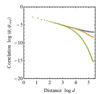
Refer to caption
Refer to caption
Refer to caption
Refer to caption
Refer to caption
Refer to caption
Figure 17: Scaling of the ψiψi+ddelimited-⟨⟩subscript𝜓𝑖subscript𝜓𝑖𝑑\langle\psi_{i}\psi_{i+d}\rangle correlator with distance d𝑑d (top) as well as the entanglement entropy SAsubscript𝑆𝐴S_{A} with subsystem length l=|A|𝑙𝐴l=|A| (bottom) at various cutoffs for the {3,6}36\{3,6\}, {3,7}37\{3,7\} and MERA tiling (left to right). The cutoffs are rc=0,50,75subscript𝑟𝑐05075r_{c}=0,50,75 ({3,6}36\{3,6\} case with 870 Majorana boundary sites), rc=0.0,0.8,0.9subscript𝑟𝑐0.00.80.9r_{c}=0.0,0.8,0.9 ({3,7}37\{3,7\} case with 876 sites), and nc=0,2,4subscript𝑛𝑐024n_{c}=0,2,4 (MERA case with 1024 sites), the data for each cutoff plotted in blue, yellow and green, respectively.

E.5 Pentagon code for quantum error correction

First, consider the boundary state of a single pentagon. Explicitly, the +11+1 logical state vector of the quantum error correcting code is given by

|0¯=Nexp(12i,jAi,j+fifj)| ,ket¯0𝑁12subscript𝑖𝑗subscriptsuperscript𝐴𝑖𝑗subscriptsuperscriptf𝑖subscriptsuperscriptf𝑗ket ,\left.\left|{\overline{0}}\right.\right\rangle=N\exp\left(\frac{1}{2}\sum_{i,j}A^{+}_{i,j}\operatorname{f}^{\dagger}_{i}\operatorname{f}^{\dagger}_{j}\right){\left.\left|{\emptyset}\right.\right\rangle}\text{ ,} (132)

with a normalization factor N=14𝑁14N=\frac{1}{4} and the 5×5555\times 5 generating matrix

A+=(0111110111110111110111110) .superscript𝐴0111110111110111110111110 .A^{+}=\left(\begin{array}[]{ccccc}\phantom{-}0&-1&\phantom{-}1&\phantom{-}1&-1\\ \phantom{-}1&\phantom{-}0&-1&\phantom{-}1&\phantom{-}1\\ -1&\phantom{-}1&\phantom{-}0&-1&\phantom{-}1\\ -1&-1&\phantom{-}1&\phantom{-}0&-1\\ \phantom{-}1&-1&-1&\phantom{-}1&\phantom{-}0\end{array}\right)\text{ .}

Correspondingly, the 11-1 logical state vector is given by

|1¯=Nexp(12i,jAi,jfifj)dηexp(ηiBifi)|~ ,ket¯1𝑁12subscript𝑖𝑗subscriptsuperscript𝐴𝑖𝑗subscriptsuperscriptf𝑖subscriptsuperscriptf𝑗d𝜂𝜂subscript𝑖subscriptsuperscript𝐵𝑖subscriptsuperscriptf𝑖~ket ,\left.\left|{\overline{1}}\right.\right\rangle=N\exp\left(\frac{1}{2}\sum_{i,j}A^{-}_{i,j}\operatorname{f}^{\dagger}_{i}\operatorname{f}^{\dagger}_{j}\right)\int\text{d}\eta\exp\left(\eta\sum_{i}B^{-}_{i}\operatorname{f}^{\dagger}_{i}\right)\widetilde{{\left.\left|{\emptyset}\right.\right\rangle}}\text{ ,} (133)

containing an integration over the auxiliary Grassmann variable η𝜂\eta, fulfilling ηfi=fiη𝜂subscriptsuperscriptf𝑖subscriptsuperscriptf𝑖𝜂\eta\operatorname{f}^{\dagger}_{i}=-\operatorname{f}^{\dagger}_{i}\eta. The generating matrix Asuperscript𝐴A^{-} and coupling matrix Bsuperscript𝐵B^{-} between η𝜂\eta and the fisubscriptsuperscriptf𝑖\operatorname{f}^{\dagger}_{i} are given by

A=(00.20.60.60.20.200.20.60.60.60.200.20.60.60.60.200.20.20.60.60.20) ,B=(11111) .formulae-sequencesuperscript𝐴00.20.60.60.20.200.20.60.60.60.200.20.60.60.60.200.20.20.60.60.20 ,superscript𝐵11111 .A^{-}=\left(\begin{array}[]{ccccc}\phantom{-}0&\phantom{-}0.2&-0.6&\phantom{-}0.6&-0.2\\ -0.2&\phantom{-}0&\phantom{-}0.2&-0.6&\phantom{-}0.6\\ \phantom{-}0.6&-0.2&\phantom{-}0&\phantom{-}0.2&-0.6\\ -0.6&\phantom{-}0.6&-0.2&\phantom{-}0&\phantom{-}0.2\\ \phantom{-}0.2&-0.6&\phantom{-}0.6&-0.2&\phantom{-}0\end{array}\right)\text{ ,}\quad B^{-}=\left(\begin{array}[]{ccccc}1&1&1&1&1\end{array}\right)\text{ .} (134)

However, we can also write this state in a purely Gaussian form by acting with annihilation operators on the fully occupied state vector |~=ifi|~ketsubscriptproduct𝑖subscriptsuperscriptf𝑖ket\widetilde{{\left.\left|{\emptyset}\right.\right\rangle}}=\prod_{i}\operatorname{f}^{\dagger}_{i}{\left.\left|{\emptyset}\right.\right\rangle},

|1¯=Nexp(12i,jAi,j+fifj)|~ .ket¯1𝑁12subscript𝑖𝑗subscriptsuperscript𝐴𝑖𝑗subscriptsuperscriptfabsent𝑖subscriptsuperscriptfabsent𝑗~ket .\left.\left|{\overline{1}}\right.\right\rangle=-N\exp\left(\frac{1}{2}\sum_{i,j}A^{+}_{i,j}\operatorname{f}^{\phantom{\dagger}}_{i}\operatorname{f}^{\phantom{\dagger}}_{j}\right)\widetilde{{\left.\left|{\emptyset}\right.\right\rangle}}\text{ .} (135)

Note that the generating matrix A+superscript𝐴A^{+} in this form is the same as for the positive-parity state, highlighting the symmetry between the positive- and negative-parity eigenstate. The additional minus sign can be removed by redefining either N𝑁N or |0~ket~0|\tilde{0}\rangle.

E.6 Higher central charges and critical scaling of entanglement entropies

By associating a higher bond dimension χ=2n𝜒superscript2𝑛\chi=2^{n} with each geometric edge, it is possible to increase the central charge c𝑐c of the conformal field theory capturing the boundary state. The corresponding 3n×3n3𝑛3𝑛3n\times 3n correlation matrix A𝐴A of each triangle state can be chosen so that correlations separate into n𝑛n parts. An example for χ=4𝜒4\chi=4 is given by

A=(00a0b0000a0ba000c00a000cb0c0000b0c 0 0) ,𝐴matrix00𝑎0𝑏0000𝑎0𝑏𝑎000𝑐00𝑎000𝑐𝑏0𝑐0000𝑏0𝑐 0 0 ,A=\left(\begin{matrix}0&0&a&0&b&0\\ 0&0&0&a&0&b\\ -a&0&0&0&c&0\\ 0&-a&0&0&0&c\\ -b&0&-c&0&0&0\\ 0&-b&0&-c&\;0\;&\;0\;\\ \end{matrix}\right)\text{ ,} (136)

where a=b=c𝑎𝑏𝑐a=b=c again corresponds to a rotation-invariant state. The construction of states with higher χ𝜒\chi is visualized in Fig. 18. Note that this separation into n𝑛n independent “channels” can only be sustained in contracted {p,q}𝑝𝑞\{p,q\} tilings if q𝑞q is even; otherwise, self-contractions lead to mixing between different channels. Also shown in Fig. 18 is the entanglement entropy scaling of the boundary states of such triangular bulks, yielding a central charge of the equivalent CFT description of c=n/2=log2χ𝑐𝑛2subscript2𝜒c=n/2=\log_{2}\sqrt{\chi}. The expected entanglement growth (11) is only reached when the subsystem size l𝑙l is larger than the size of one geometrical edge, i.e. 2n2𝑛2n Majorana fermions. Indeed, by construction of our Gaussian model, a site of one Majorana fermion always has an entanglement entropy of 1/2log21221/2\log 2, independent of χ𝜒\chi.

Refer to caption
Refer to caption
Figure 18: Left: Construction of triangle states with bond dimension χ=2,4,8𝜒248\chi=2,4,8. Colored connections between boundary sites {θi}subscript𝜃𝑖\{\theta_{i}\} denote non-zero correlations. Right: Mean value of entanglement entropy 𝔼(S)=subscript𝔼𝑆absent\mathbb{E}_{\ell}(S)= k=1LS[k,k+]superscriptsubscript𝑘1𝐿subscript𝑆𝑘𝑘\sum_{k=1}^{L}S_{[k,k+\ell]} of a boundary subsystem of size \ell. Results for {3,8}38\{3,8\} tiling with bond dimension χ=2,4,8𝜒248\chi=2,4,8 (bottom to top; with 144,288,432144288432144,288,432 Majorana fermions, respectively).

References

  • Maldacena (1998) J. M. Maldacena, Adv. Theor. Math. Phys. 2, 231 (1998).
  • van Raamsdonk (2010) M. van Raamsdonk, Gen. Rev. Grav. 42, 2323 (2010)arXiv:1005.3035 .
  • Pastawski and Preskill (2017) F. Pastawski and J. Preskill, Phys. Rev. X 7, 021022 (2017)arXiv:1612.00017 .
  • Eisert et al. (2010) J. Eisert, M. Cramer,  and M. B. Plenio, Rev. Mod. Phys. 82, 277 (2010).
  • Ryu and Takayanagi (2006) S. Ryu and T. Takayanagi, Phys. Rev. Lett. 96, 181602 (2006).
  • Swingle (2012) B. Swingle, Phys. Rev. D 86, 065007 (2012).
  • Vidal (2008) G. Vidal, Phys. Rev. Lett. 101, 110501 (2008).
  • Evenbly and Vidal (2009) G. Evenbly and G. Vidal, Phys. Rev. B 79, 144108 (2009).
  • Dawson et al. (2008) C. M. Dawson, J. Eisert,  and T. J. Osborne, Phys. Rev. Lett. 100, 130501 (2008).
  • Almheiri et al. (2015) A. Almheiri, X. Dong,  and D. Harlow, JHEP 1504, 163 (2015).
  • Lee and Qi (2016) C. H. Lee and X. L. Qi, Phys. Rev. B 93 (2016), 1503.08592 .
  • Pastawski et al. (2015) F. Pastawski, B. Yoshida, D. Harlow,  and J. Preskill, JHEP 2015, 149 (2015).
  • Hayden et al. (2016) P. Hayden, S. Nezami, X.-L. Qi, N. Thomas, M. Walter,  and Z. Yang, J. High En. Phys. 2016, 9 (2016).
  • Valiant (2002a) L. G. Valiant, SIAM J. Comp. 31, 1229 (2002a).
  • Bravyi (2009) S. Bravyi, Cont. Math. 482, 179 (2009).
  • Evenbly and White (2016) G. Evenbly and S. R. White, Phys. Rev. Lett. 116, 140403 (2016).
  • Haegeman et al. (2018) J. Haegeman, B. Swingle, M. Walter, J. Cotler, G. Evenbly,  and V. B. Scholz, Phys. Rev. X 8, 011003 (2018).
  • Evenbly (2017) G. Evenbly, Phys. Rev. Lett. 119, 141602 (2017).
  • Evenbly and Vidal (2015a) G. Evenbly and G. Vidal, Phys. Rev. Lett. 115, 180405 (2015a).
  • Evenbly and Vidal (2015b) G. Evenbly and G. Vidal, Phys. Rev. Lett. 115, 200401 (2015b).
  • Orus (2014) R. Orus, Ann. Phys. 349, 117 (2014).
  • Schuch (2013) N. Schuch, Lecture notes for the 44th IFF Spring School “Quantum Information Processing” in Juelich  (2013).
  • Verstraete et al. (2008) F. Verstraete, J. I. Cirac,  and V. Murg, Adv. Phys. 57, 143 (2008).
  • Eisert (2013) J. Eisert, Mod. Sim. 3, 520 (2013).
  • Berezin (1966) F. Berezin, The method of second quantization (Academic Press, 1966).
  • Cahill and Glauber (1999) K. E. Cahill and R. J. Glauber, Phys. Rev. A 59, 1538 (1999).
  • Bravyi (2005) S. Bravyi, Quantum Inf. and Comp. 5, 216 (2005).
  • Terhal and DiVincenzo (2002) B. M. Terhal and D. P. DiVincenzo, Phys. Rev. A 65, 032325 (2002).
  • Laflamme et al. (1996) R. Laflamme, C. Miquel, J. P. Paz,  and W. H. Zurek, Phys. Rev. Lett. 77, 198 (1996).
  • Gottesman (1996) D. Gottesman, Phys. Rev. A 54, 1862 (1996).
  • Terhal (2015) B. M. Terhal, Rev. Mod. Phys. 87, 307 (2015).
  • Gottesman (1997) D. Gottesman,   (1997), arXiv:quant-ph/9705052 [quant-ph] .
  • Holzhey et al. (1994) C. Holzhey, F. Larsen,  and F. Wilczek, Nucl. Phys. B 424, 443 (1994).
  • Calabrese and Cardy (2004) P. Calabrese and J. Cardy, J. Stat.Mech. 0406, P06002 (2004).
  • Ware et al. (2016) B. Ware, J. H. Son, M. Cheng, R. V. Mishmash, J. Alicea,  and B. Bauer, Phys. Rev. B 94, 115127 (2016).
  • Balasubramanian and Ross (2000) V. Balasubramanian and S. F. Ross, Phys. Rev. D61, 044007 (2000)arXiv:hep-th/9906226 [hep-th] .
  • Caputa et al. (2017) P. Caputa, N. Kundu, M. Miyaji, T. Takayanagi,  and K. Watanabe, Phys. Rev. Lett. 119, 071602 (2017)arXiv:1703.00456 [hep-th] .
  • Barthel et al. (2009) T. Barthel, C. Pineda,  and J. Eisert, Phys. Rev. A 80, 042333 (2009).
  • Corboz et al. (2010) P. Corboz, R. Orus, B. Bauer,  and G. Vidal, Phys. Rev. B 81, 165104 (2010).
  • Kraus et al. (2010) C. V. Kraus, N. Schuch, F. Verstraete,  and J. I. Cirac, Phys. Rev. A 81, 052338 (2010).
  • Wille et al. (2017) C. Wille, O. Buerschaper,  and J. Eisert, Phys. Rev. B 95, 245127 (2017).
  • Bultinck et al. (2017) N. Bultinck, D. J. Williamson, J. Haegeman,  and F. Verstraete, Phys. Rev. B 95, 075108 (2017).
  • Valiant (2002b) L. G. Valiant, SIAM J. Comp. 31, 1229 (2002b).
  • Temperley and Fisher (1961) H. N. V. Temperley and M. E. Fisher, Phil. Mag. 6, 1061 (1961).
  • Kasteleyn (1961) P. Kasteleyn, Physica 27, 1209 (1961).
  • Cai et al. (2007) J.-Y. Cai, V. Choudhary,  and P. Lu, in Computational Complexity, 2007. CCC’07. Twenty-Second Annual IEEE Conference on (IEEE, 2007) pp. 305–318.
  • Bloch and Messiah (1962) C. Bloch and A. Messiah, Nucl. Phys. 39, 95 (1962).
  • Kraus (2009) C. V. Kraus, A quantum information perspective of fermionic quantum many-body systems, Ph.D. thesis, Universität München (2009).
  • Bravyi and Gosset (2016) S. Bravyi and D. Gosset, arXiv:1609.00735  (2016).
  • Francesco et al. (1997) P. Francesco, P. Mathieu,  and D. Senechal, Conformal Field Theory (Springer, 1997) pp. 439–486.
  • Serafini et al. (2004) A. Serafini, F. Illuminati,  and S. De Siena, J. Phys. B37, L21 (2004)arXiv:quant-ph/0307073 [quant-ph] .