Recursive Neural Networks in Quark/Gluon Tagging

Abstract

Since the machine learning techniques are improving rapidly, it has been shown that the image recognition techniques in deep neural networks can be used to detect jet substructure. And it turns out that deep neural networks can match or outperform traditional approach of expert features. However, there are disadvantages such as sparseness of jet images. Based on the natural tree-like structure of jet sequential clustering, the recursive neural networks (RecNNs), which embed jet clustering history recursively as in natural language processing, have a better behavior when confronted with these problems. We thus try to explore the performance of RecNNs in quark/gluon discrimination. The results show that RecNNs work better than the baseline boosted decision tree (BDT) by a few percent in gluon rejection rate. However, extra implementation of particle flow identification only increases the performance slightly. We also experimented on some relevant aspects which might influence the performance of the networks. It shows that even taking only particle flow identification as input feature without any extra information on momentum or angular position is already giving a fairly good result, which indicates that the most of the information for quark/gluon discrimination is already included in the tree-structure itself. As a bonus, a rough up/down quark jets discrimination is also explored.

1 Introduction

The study of jet substructure has been the very advanced topic in jet physics at the Large Hadron Collider (LHC). The techniques in distinguishing different substructures have been established well Larkoski:2017jix ; Adams:2015hiv . And at this stage, different jet observables have been invented to improve our understanding about jets. As for application, we can use jet substructure to detect new physics such as Supersymmetry or Two Higgs Doublet Models. For theoretical development, demand on theoretical calculation of jet substructure observables actually pushes our precision calculation forward and helps us understand QCD better. And the development of Monte Carlo tools also interacts with jet measurements at the LHC.

When the experimental environment gets more complex and the problem has larger and larger dimension, the number of observables we need is increasing, and sometimes gets so large that exceeds our actual computation capability . Artificial neural networks have already been employed for high dimensional problems. Earlier research using neural networks are carried out in a framework of designing observables by hand at first and then feeding these observables into neural networks to do classification. It strongly relies on the pre-stage of expert-features designing, and thus depends on physicists’ understanding on the problem. The expert-feature approach has a very long history in high energy physics, but there are several pros and cons. They generally have clear physical intuition. The observables are designed according to physical understanding and theoretical insights. And their behavior are well understood, and based on theoretical framework. However, they can only deal with problems case by case, and highly depend on the specific processes worked with. And there are always strong correlation between observables. At last, since we are not guaranteed that all the information can be captured in the observables, the best we can do is just approaching the limit by trial and error. And there is no guide for how much information we have captured.

Along with the new framework in machine learning (ML) getting more and more mature, relevant techniques have been employed in high energy physics. The new machine learning framework augmented our ability to fully utilize experimental data. On one hand, the input data can be taken from the raw detector measurements, which means we don’t have to lose information because of data transformation or specific observable designing. On the other hand, this new input formulation also brings new insights on how we organize our observations. Finally, the uniform formulation and general approach might help us out of the busy tasks of too-many-sub-channels designing. Especially for jets and their structure analysis, we have the opportunity to improve our working culture to adapt to the ML era.

There have already been some works using deep neural networks (DNN) in jet physics. The very first attempt was made in using computer vision Cogan:2014oua to help with jet tagging. And later people started to use image recognition in boosted top tagging Almeida:2015jua ; Pearkes:2017hku ; Kasieczka:2017nvn , boosted W tagging Baldi:2016fql , heavy flavour classification Guest:2016iqz , and the investigation of parton shower uncertainties is also made Barnard:2016qma . A detailed report on image recognition in jet substructure is given in reference deOliveira:2015xxd . And more interestingly, colored version of image recognition inspired by particle flow has also been proposed Komiske:2016rsd . Based on all these recent development, it can be shown that deep neural networks generally match or outperform the conventional expert feature approach. And the colored version can perform better than gray scale in some cases since it employs more information. The basic idea of image recognition in jet physics is mapping a jet onto the $({\rm azimuthal~{}angle}~{}\eta,~{}{\rm pseudorapidity}~{}\phi)$ plane and translating the transverse momentum $p_{T}$ of every constituent of the jet into intensity of the pixel. Thus the higher $p_{T}$, the darker the pixel will be. By feeding these jet images after some preprocessing into deep neural networks, we can discriminate signal from background with the raw data from the detector while avoiding too much human designing on the physics problem. And at experiments, CMS has already carried out heavy flavor identification using DNN recently CMS-DP-2017-005 .

Until now, most of the work is done in the regime of image recognition, since it is the most intuitive, simple and general approach. However, there are some disadvantages for image recognition:

• sparseness: in most cases only 5%-10% pixels are active in jet images of fixed size deOliveira:2015xxd . Thus most of the parameter space is actually wasted.

• the pixelization process causes information loss.

• computation cost: too many model parameters require more computation power. Not very efficient for larger image size.

• it’s more complicated to do the event-level analysis. Of course one can channel the output of image classifier into later classifier based on expert features or other network architecture, but that will anyway bring some complication and detailed investigation is necessary.

Aside from image recognition, another natural approach is recurrent neural networks (RNN) Goodfellow-et-al-2016 , which takes sequences as input and is widely used in natural language processing. RNN adapts to the problems confronted in image recognition better since it can properly deal with sequential input of variable length. And also the parameter sharing makes it very efficient. To be more concrete, a recurrent network is structured as a recurrent chain, in which every step takes in the output of the last computation, and all the steps share the same set of parameters. Recursive Neural Networks (here abbreviated as RecNN in order not to be confused with recurrent neural networks), rather, has a tree-like structure, other than the chain-like one of RNN. Respect to RNN, RecNN reduces the computation depth from $\tau$ to $\mathcal{O}(\log\tau)$. As an example, RNN is explored in Guest:2016iqz for heavy flavor tagging, by taking low level track and vertex information as input for the neural networks.

Base on the natural analogy of the sequentially clustered jet and the input structure of RecNN, a group Louppe:2017ipp has implemented the RecNN version of jet analysis. In their work, the framework is built for embedding jet recursively into a root jet node, and then feeding it into the sequential classifier. And by a simple extension, event-level analysis can be easily implemented in a structure-in-structure manner, although right now only dealing with jets-only events with very limited application range. The work is done in the regime of jet substructure for boosted gauge boson. And the results show that the RecNN outperforms the expert feature approach and image version in DNN.

Motivated by all these progresses and the prospects, we try to explore the performance of RecNN in another very interesting topic: quark/gluon discrimination. Quark/gluon tagging is gaining great potential at the LHC. Since gluon has a larger color factor than quarks, gluon jets will generally have more radiation and also broader radiation pattern. The ratio of final state counts for gluon and quark jets is predicted by an asymptotic value of 9/4. The measurements at the LHC Aad:2016oit also support this prediction, where the charged particle multiplicity is measured, and shows the tendency of approaching the limit.

Figure 1: Distributions of jet scaled mass, girth, and track count for quark and gluon jets with $p_{T}=$ 1 TeV.

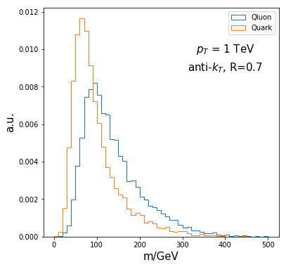
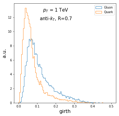
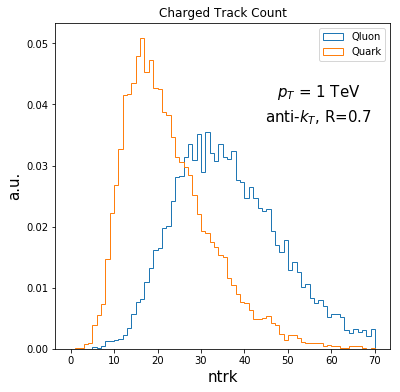
The conventional approach in quark/gluon discrimination is defining some jet observables, such as charge multiplicity, jet mass, jet subjettiness Gallicchio:2012ez (Fig. 1 shows the distributions of a few observables for 1 TeV quark and gluon jets). These jet observables have turned to be very efficient and well-motivated discriminants. For a multivariable analysis, the general performance is: for a 50% quark acceptance, the gluon rejection can reach 80 % - 90 %, and the corresponding significance can have an increase by a factor of 2 - 3. These results show a great potential in helping new physics search, and thus the exploration in DNN which can make use of all the low level information is worthwhile. The image approach using Convolutional Neural Networks (CNN) has been explored Komiske:2016rsd , showing performance matching or outperforming conventional expert feature approach. And the DNN simulation from ATLAS ATL-PHYS-PUB-2017-017 and CMS CMS-DP-2017-027 using either CNN or RNN also confirm the potential. For a 50% quark acceptance at jet $p_{T}\sim 200$ GeV, mis-identification rate is approximately $10\%$ (a few percent away from the pythia-level results).

In this work, we aim to address the following questions:

• At first, how does the RecNN generally perform in quark/gluon discrimination at the LHC.

• We include fast detector simulation in our analysis, trying to bring a more realistic picture to the problem.

• How to better implement particle flow identification in RecNN, in order to gain a more containing information set.

The paper is organized as following: in Section 2, we describe in detail the process of jet embedding and the neural network architecture. Then we explore the RecNN performance in quark/gluon discrimination in Section 3. Besides, a brief investigation in up/down quark discrimination using RecNN is also presented in Section 3. Conclusions are given in Section 4. And finally a short discussion and outlook in Section 5 is presented.

2 Methodology

2.1 Jets at the LHC

There are several different definitions Gras:2017jty of a ”jet”. How to connect the theoretical parton and the experimental measurements on a collimated spray of hadrons is not a trivial problem. But in practice, the jet is operationally defined by the jet algorithm used to group particles into clusters.

The basic idea of sequential jet clustering Salam:2009jx is to recombine the particles into pseudojets recurrently according to some measure and recombination scheme. The “closest” particles will be combined into pseudojets at first. And by this QCD-inspired measure, we can get soft and collinear safe jet definition. And through this recursive clustering process, the global information including number of particles, their momenta, clustering history, is embedded in the tree structure of the clustering sequence.

Here shows the typical tree-structures of a 1 TeV gluon jet and quark jet in Fig. 2.

Figure 2: Typical tree structures for 1 TeV gluon jet (left) and quark jet (right).

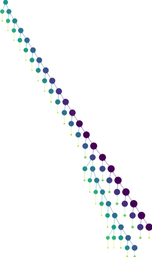
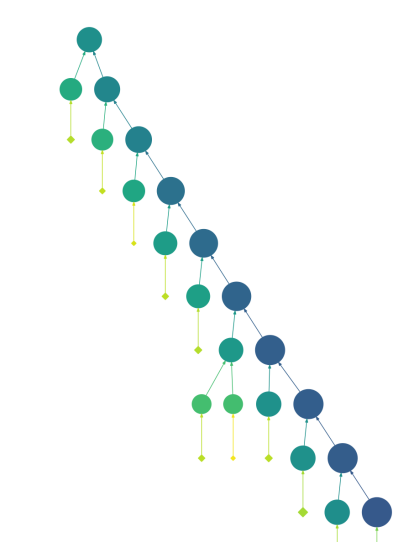
A naive impression is that the gluon jet has more constituents and accordingly more complicated clustering structure. Actually the mean content number of a 1 TeV gluon jet is $\sim$ 90, while for a quark jet is approximately 50. And the typical number of charged constituents for a 1 TeV gluon jet is 36, and for a quark jet is 22. Thus if we input all the measured degrees of freedom (d.o.f.) into analysis, for every final state particle we have 3 d.o.f. ($p_{T}$, $\eta$ and $\phi$) and one more if particle flow identification is taken into account, thus for a whole jet the total d.o.f can reach $\sim 4\times 100$. If we want to utilize all the information we’ve gotten, such high dimensionality naturally brings us to the DNN approach, although there are arguments about how much information actually is included in a jet Datta:2017rhs .

2.2 Network Architecture

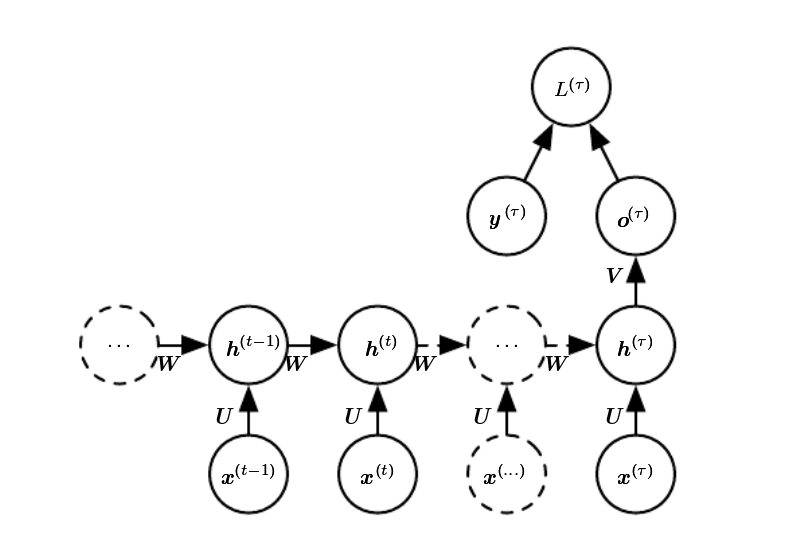
Here first gives a short introduction to RNN. Recurrent neural networks are initially designed for processing sequential data. The state of the system is recurrently defined. For the t-th step, the state ${\bf h}^{(t)}$ is defined by the output of last step and the new feed as:

$$\textbf{h}^{(t)} = g^{(t)}(x^{(t)},x^{(t-1)},...,x^{(1)})$$ (1)

$$= f(h^{(t-1)},x^{(t)};\theta)$$

where the same transition function f is applied for every step. Thus this parameter sharing makes the model very simple and efficient. And the recursive networks, rather, use a tree-structure instead of a chain-like structure. As shown in the right part of Fig. 3, the matrices W, U and V are shared parameters by all the steps. In Fig. 3, unfolded computational graphs of a typical RNN and a RecNN are depicted. And there is one hidden-to-output at the end of the sequence. This output can be a final loss function or can be fed into following classifier. In brief, it summarizes a sequence and gives a fixed-length representation.

Figure 3: Left: Time-unfolded computational graph for a RNN which only takes the output at the end of the sequence. Right: Time-unfolded computational graph for a RecNN. Plots are taken from Ref. Goodfellow-et-al-2016 with permission.

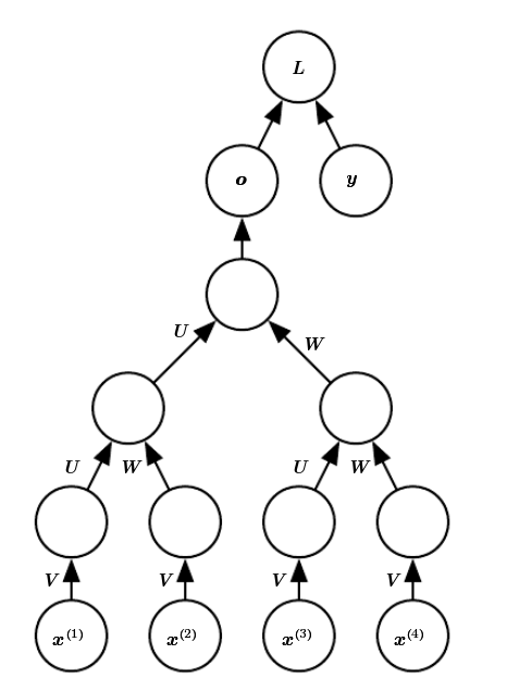
Based on the similarity between jet clustering and RecNN architecture, the application of RecNN is straightforward. The raw data from detector can be used as direct input to the networks. The measured transverse momentum $p_{T}$ and the angular location ($\eta,~{}\phi$) give the basic feature set. After a regular jet clustering process, the jet (defined by the clustering structure t with its contents $\{v_{i},i=1,..,N_{j}\}$, where $v_{i}$ denotes the four-momentum vector of i-th particle within the jet) is embedded recursively into an embedding space of fixed size, then the embedded jet node will be channeled to following classifier (a MLP).

According to Ref. Louppe:2017ipp , a jet is recursively embedded into a single jet node ${\bf h}^{\rm jet}_{1}$. And through this recursive embedding, the history of jet clustering can be included in the final jet node. The procedure of embedding is a mapping from the feature space (with dimension f) to the embedding space (with dimension q) $R^{f}\to R^{q}$. For every jet with $N_{j}$ constituents, there are $2N_{j}-1$ clustering nodes. Every node is represented by an input vector in the embedding space ${\bf u}\in R^{q}$ after a transformation from feature vector x (generally can be defined as ($p_{T}$, $\eta$, $\phi$) or other version with the same information contents) as following:

$$\textbf{u}_{k}=\sigma(W_{u}{\bf x}_{k}+b_{u})~{}\,\textrm{ for~{}the~{}k-th~{}node~{}~{}}$$ (2)

where $W_{u}\in R^{q\times f}$, $b_{u}\in R^{q}$ and $\sigma$ denotes the ReLU activation function.

Then, the embedding of every node is defined by its children and its own input feed (we can also define the embedding by simply using the children. This version is also explored and shows similar performance while reducing the model parameters, see discussion in the next section):

$$\textbf{h}_{k}=\sigma\left(W_{h}\left[\begin{array}[]{c}\textbf{h}^{\rm jet}_{k_{L}}\\ \textbf{h}^{\rm jet}_{k_{R}}\\ \textbf{u}_{k}\end{array}\right]+b_{h}\right)$$ (3)

where we have model parameters $W_{h}\in R^{q\times 3q}$, $b_{h}\in R^{q}$. $k_{L}$ and $k_{R}$ are left and right child of node k respectively. Down to the leaves (the original jet constituents), we have directly ${\bf h}_{k}={\bf u}_{k}$. Thus, combining the raw input of detector measurements and jet clustering history, we can embed the information finally into a single root jet node ${\bf h}_{1}$, which is passed to a following classifier for final classification. All the embedding parameters ($W_{u}$, $b_{u}$, $W_{h}$ and $b_{h}$) are learned using backpropagation jointly with the parameters of the following classifier $W_{\rm clf}{\rm~{}and~{}}b_{\rm clf}$, by trying to minimize the loss function.

The procedure is depicted as following:

$$[\{{\bf t},\{v_{i},i=1,..,N_{j}\}\}\to{\bf h}^{\rm jet}\in R^{q}]\to{\rm ReLU}\to{\rm ReLU}\to{\rm Sigmoid}~{}\,$$ (4)

where the rectified linear unit pmlr-v15-glorot11a (ReLU) $={\rm max}\{0,z\}$ is used for the hidden layers in the classifier, and Sigmoid ($\frac{1}{1+e^{-z}}$) activation is used for the output layer. And the log loss function is employed:

$$L=-\frac{1}{N}\sum_{i}^{N}(y_{i}\log(y_{i}^{pred})+(1-y_{i})\log(1-y_{i}^{pred}))~{}\,$$ (5)

where $y_{i}$ is the label for i-th jet, and $y_{i}^{pred}$ is the prediction of the model.

Recursively defined jet charge:

Other than the very basic input set ($p_{T}$, $\eta$, $\phi$), more information can be included. At the LHC, the particle flow algorithm Sirunyan:2017ulk combines the information through different parts of the detector thus gives more identification ability. It can match tracks to the energy deposit in the calorimeters, thus we have more accurate knowledge about the final states, and also higher precision on their transverse momenta. Right now, we can identify charged tracks, neutral particles and photons within one jet. But how to implement this information in RecNN deserves some exploration. They can be implemented in a naive way as one-hot vectors (($i_{\rm neutral~{}hadron}$, $i_{\rm photon}$, $i_{\rm+}$, $i_{\rm-}$), $i=0~{}{\rm or}~{}1$, activated by the particle flow identification, e.g., a photon is represented by (0, 1, 0, 0)) added to the feature vector. However, since the one-hot implementation doesn’t have an additive nature (or, the particle flow identification of the inner nodes is not well-defined), the recursive embedding can’t utilize this information effectively. In Ref. Louppe:2017ipp , the authors claimed that including particle flow identification wouldn’t gain any significant improvement for their attempt in discriminating boosted W jets and QCD jets.

In order to search for a better way to implement the particle flow identification, we ask help from a jet observable: jet electric charge. Jet charge is a very useful observable for identifying jet flavor and the identification of W’ and Z’. The pt-weighted jet charge Field:1977fa ; Krohn:2012fg is defined as following:

$$Q_{\kappa}^{J}=\sum_{i\in J}(\frac{p_{T}^{i}}{p_{T}^{J}})^{\kappa}q_{i}~{},$$ (6)

where $q_{i}$ is the electric charge of the particle within the jet, and $p_{T}^{i}$ is the transverse momentum of the component, while $p_{T}^{J}$ denotes the total transverse momentum of the jet. $\kappa$ is a free parameter, and $\kappa\to 0$ gives the limit of simply adding charges of the components while $\kappa\to\infty$ gives the limit of the charge of the hardest component. The typical value has been used by experiments lies between 0.2 and 1.0.

Trying to carry the particle flow information in the RecNN, we construct the recursively defined pt-weighted charge for the clustering tree:

$$Q_{k}^{\rm rec}=\frac{Q_{k_{L}}^{\rm rec}(p_{T}^{k_{L}})^{\kappa}+Q_{k_{R}}^{\rm rec}(p_{T}^{k_{R}})^{\kappa}}{(p_{T}^{k})^{\kappa}}~{}\,$$ (7)

while for the leaves $Q_{k}^{\rm rec}=q_{i}$. The pt-weighted charge of k-th node $Q_{k}^{\rm rec}$ is defined by its children in the same manner as in Eqn. 6. In this way, we still get the right pt-weighted charge for the jet node at the end of the embedding. This $Q_{k}^{\rm rec}$ along with the traditional feature set contributes to an almost-complete set of the information we get from detectors. $\kappa=0.5$ will be used throughout this work.

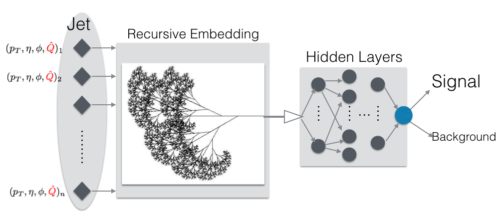
Prepared with all the basic settings, we depict the whole architecture in Fig. 4.

Figure 4: Workflow including jet embedding and the following classification (schematic plot of the recursion is credited to Brentsmith101 under Wikimedia Commons).

2.3 Setup

HEP Data Preparation:

In preparing sample jets, Pythia8 Sjostrand:2014zea is used to generate events and carry out the parton shower and the following haronization. Delphes deFavereau:2013fsa is used for fast detector simulation (pile-up effects are left aside for the time being). Jets are first clustered using FastJet Cacciari:2011ma with anti-kt algorithm Cacciari:2008gp . After preprocessing, the constituents within one jet will be reclustered and then the four-momenta of the particles in a jet along with the clustering tree will be passed into RecNN embedding as described in the previous subsection. And the data is generally formatted in hd5f using interfaces in deepjets Barnard:2016qma . The details concerning processes used for sample signal and background jets, and other parameters are described in the next section.

Preprocessing:

Before being fed into the RecNN embedding, some basic preprocessing steps are applied to the jet samples. We only apply the necessary translation and rotation to extract ”pure“ jets disconnected to the rest of the event.

• translation: jets are translated to be centered at $(\eta,\phi)=(0,0)$.

• rotation: the jet is rotated in the ($\eta,\phi$) plane such that the energy deposition axis is the same (here is (1,0)) for all samples in order to eliminate the effects of global influence from color connections with the remnants of the event (but it will be very interesting that we have a solution on event level which takes the color connections seriously). Thus only the intra-jet correlation is used for analysis. The rotation reads as:

  $$\eta =\hat{\eta}\cos\alpha+\hat{\phi}\sin\alpha$$ (8)

  $$\phi =-\hat{\eta}\sin\alpha+\hat{\phi}\cos\alpha$$ (9)

  where the rotation angle $\alpha$ is defined by the ”principal axis” Almeida:2015jua :

  $$\tan\alpha=\frac{\sum_{i}\frac{\hat{\phi}_{i}E_{i}}{\Delta\hat{R}_{i}}}{\sum_{i}\frac{\hat{\eta}_{i}E_{i}}{\Delta\hat{R}_{i}}}$$ (10)

Neural Networks Setup:

The training is carried out with library Scikit-learn scikit-learn and the RecNN framework built by Louppe:2017ipp . And the subsequent classifier we are using consists of two hidden layers with rectified linear unit (ReLU) activations, and the final output node is equiped with sigmoid activation. And the Adam DBLP:journals/corr/KingmaB14 algorithm is employed for the minimization.

The input feature vector finally fed into the networks is ${\bf x}_{i}=(p_{i},\eta_{i},\phi_{i},E_{i},E_{i}/E_{J},p_{Ti},\theta_{i}=2\arctan(\exp(-\eta_{i})))$. The dimension of embedding space is set to be 40 (which has been proven to be large enough for the case we are examining and also not too large to preserve computation time). The training is done through 10 epoches with the batch size of 64. The learning rate is set to be 0.0005 initially and is decayed linearly by a rate of 0.9 for every epoch. The training set consists of 50,000 - 100,000 (the exact number depends on the case) data samples and among which 5,000 is used as validation set to prevent overfitting. And the performance is tested with a dataset of 10,000 - 20,000 samples.

3 Results

In this section we show the performance of RecNN on the task of discriminating quark/gluon (q/g) jets. And some effects from variants are discussed. As a byproduct, we also explored the first step on (light-)jet flavor identification in Subsection 3.2.

We show here the discrimination power in use of Receiver Operating Characteristic (ROC) curve, which is the standard measure (1/(false positive rate) v.s true positive rate) and sometimes is plotted as the signal efficiency v.s. background rejection rate (i.e., 1 - false positive rate) for a more intuitive presentation. The Area Under the Curve (AUC) of ROC is the overall metric to measure the performance. Generally, the larger the AUC, the better the performance. And as baseline, we also give the Boosted Decision Tree (BDT) results using expert features as input.

3.1 Quark/Gluon Discrimination

The processes used to sample jets are $q\bar{q}\to gg$ and $gg\to gg$ for gluon jets, and $gg\to q\bar{q}$, $q\bar{q}\to q\bar{q},qq\to qq$ for light quarks (u,d,s), at $\sqrt{s}=13$ TeV. A set of benchmark jet $p_{T}$s are examined. The $p_{T}$ bins are set to be: [90,110], [180, 220], [480, 520], [950, 1050] (in GeV). Jets are clustered using anti-kt algorithm Cacciari:2008gp and cone size is set to be $R=0.7$ for high $p_{T}$ ($p_{T}=1$ TeV) and $R=0.4$ for other relatively lower $p_{T}$s.

The performace for different simulation levels are explored: pythia level, delphes e-flow and delphes towers. According to our experiments, using only towers can’t provide significant discrimination for q/g, thus we don’t put the results here. For pythia level analysis, we employ the constraints of $|\eta|<2.5$, and discard neutrinos before clustering.

We first investigated the RecNN performance with the architecture indicated in the previous section, ROCs are shown and comparison with image approach (CNN) and BDT is also carried out. The baseline BDT is composed of scaled mass ($m_{J}/p_{T}$), charged particle multiplicity, and girth ($g=\sum_{i\in{\rm Jet}}\frac{p_{T}^{i}}{p_{T}^{J}}r_{i}$). For adding information of particle flow, three scenarios are considered: 1) without extra particle flow identification; 2) with one-hot vector implementation of particle flow identification; 3) with recursively defined pt-weighted charge $Q^{\rm rec}$ instead. Then the jet-$p_{T}$ dependence is studied. Furthermore, we explored the behavior of several variants: changing cone size for jet clustering; modification of the input feature set; modification of the embedding feed; etc.

To show the physical implications more clearly, the acceptance and rejection rate can be translated into a significance improvement (SI) factor for any working point as:

$$\sigma\equiv\frac{S}{\sqrt{B}}~{}\to~{}\frac{\epsilon_{S}S}{\sqrt{\epsilon_{B}B}}=\left(\frac{\epsilon_{S}}{\sqrt{\epsilon_{B}}}\right)\sigma~{}\to~{}{\rm SI}=\frac{\epsilon_{S}}{\sqrt{\epsilon_{B}}}$$ (11)

Thus, the ROCs can be mapped into significance improvement curves (SICs) Gallicchio:2010dq . We also show the corresponding SICs in the following.

	Gluon Jet Efficiency (%) at 50 % Quark Jet Acceptance	200 GeV	1000 GeV
Pythia	BDT of all jet variables	5.2∗	5.2∗
	Deep CNN without Color	4.8∗	4.0∗
	Deep CNN with Color	4.6∗	3.4∗
	RecNN without pflow	6.4	4.5
Delphes	BDT	9.5	6.2
	RecNN without pflow	7.8	4.6
	RecNN with categorical pflow	7.1	4.5
	RecNN with pt-weighted charge	7.8	4.9
Full Sim.	DNN@CMS	$\sim$10.0†	–

Table 1: Results displayed for different scenarios for comparison. Data with ^∗ is CNN results taken from Ref. Komiske:2016rsd , and data with ^† is take from CMS-DP-2017-027 (with extrapolation) for quick comparison. In the upper part, we show the particle level (pythia level) results; and in the lower part, detector simulation is included, thus generally reduces the discrimination power a bit.

In Table 1, we present the gluon efficiency at the working point of 50% quark acceptance, at benchmarks $p_{T}=200,1000$ GeV. We first show the results for pythia level in the upper part of the table. And the performance after detector simulation is shown in the lower part.

In Pythia-level, we also take numbers from Ref. Komiske:2016rsd for CNNs (pythia level) as a quick comparison. From the numbers, RecNN is not working much better, but still matches the previous results from BDT and CNN. In Delphes-level, the RecNN is still giving excellent performance after fast detector simulation. And compared to pythia level, the delphes level got more influence from $p_{T}$. The decrease in jet $p_{T}$ reduces the performance much quicker. The detector responses at different $p_{T}$s deserve more careful investigation. The numbers show that RecNNs are obviously surpassing BDT and there is a potential for full detector simulation. In Ref. CMS-DP-2017-027 , CMS Collaboration has carried out full simulation in DNNs for q/g tagging (CMS Collaboration has done the simulation within three different DNN architectures: DeepJet, LSTM, CNN). We put the number from there (with extrapolation. Since the three DNN architectures give similar results for the relevant benchmark working point, we only show one representative number for them.) in Table 1 as reference.

For CNNs within image recognition approach, the particle flow information implemented in colored channels Komiske:2016rsd (where the detector effects are not taken into account) gives slight improvement for high $p_{T}$ jets (500 GeV - 1 TeV) (for $p_{T}=1$ TeV, the gluon efficiency drops from 4.0% to 3.4% for working point of 50% quark acceptance, and the best SI increases by a factor of 1.2), while leaving performance on low $p_{T}$ jets not much changed. Since the particle flow is actually a concept closely related to detector structure, we only consider the implementation of particle flow after fast simulation using Delphes. With extra particle flow information implemented in either one-hot vectors or recursively defined pt-weighted jet charge, the performance is not improved much (although there is a slight increase. And in contrast to CNN, here the increase is more visible for relatively lower jet $p_{T}$s. See Table. 2 for detailed numbers), as claimed in Louppe:2017ipp for W tagging. This might indicate that by taking particle four-momenta directly as input, RecNN is already fully extracting information for q/g tagging. Actually the investigation on input features in later part of this section will also confirm that there is information saturation.

Figure 5: ROCs (left) and SICs (right) for jet $p_{T}=1$ TeV. Baseline BDT and three scenarios concerning particle flow information are displayed.“nopflow”: no extra particle flow identification is added to RecNN; “one-hot”: one-hot implementation of particle flow; “ptwcharge”: recursively defined pt-weighted charge implemented in the embedding process.

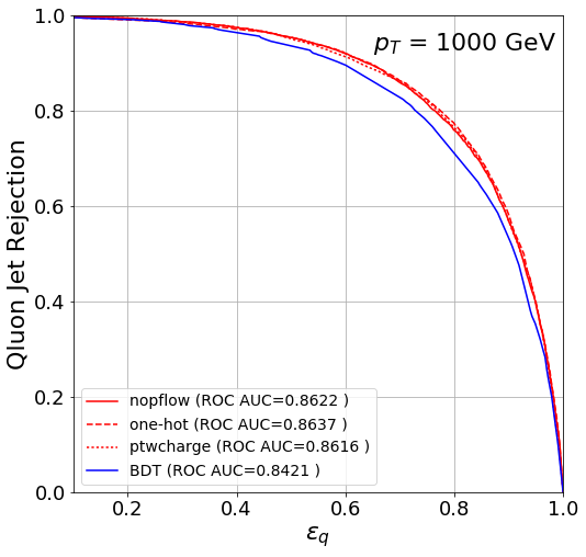
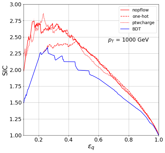
In Fig. 5, the ROCs and corresponding SICs for benchmark transverse momentum $p_{T}=1$ TeV are displayed. On the left panel, we show the ROCs curves for RecNNs and the baseline BDT. For a signal efficiency of 50%, the $\sim 95\%$ background can be rejected. The three RecNNs give better performance than BDT. And for a signal efficiency of 80%, the mis-identification rate is about 23%. On the right hand side of Fig. 5, we show the SICs. The significance can be improved by a factor of $\sim$2.75 (best SI) for a signal efficiency of 0.2 - 0.3, and by a factor of $\sim$1.7 for $\epsilon_{S}=0.8$.

Figure 6: ROCs of RecNNs for various jet $p_{T}$s: 200 GeV, 300 GeV, 500 GeV, and 1 TeV. Notations are the same as in Fig. 5.

Figure 7: SICs of RecNNs for various jet $p_{T}$s: 200 GeV, 300 GeV, 500 GeV, and 1 TeV. Notations are the same as in Fig. 5.

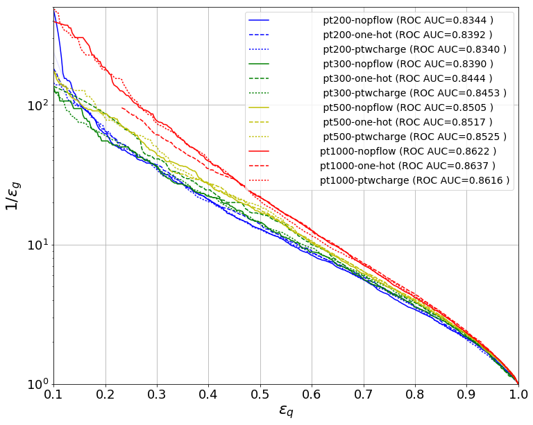
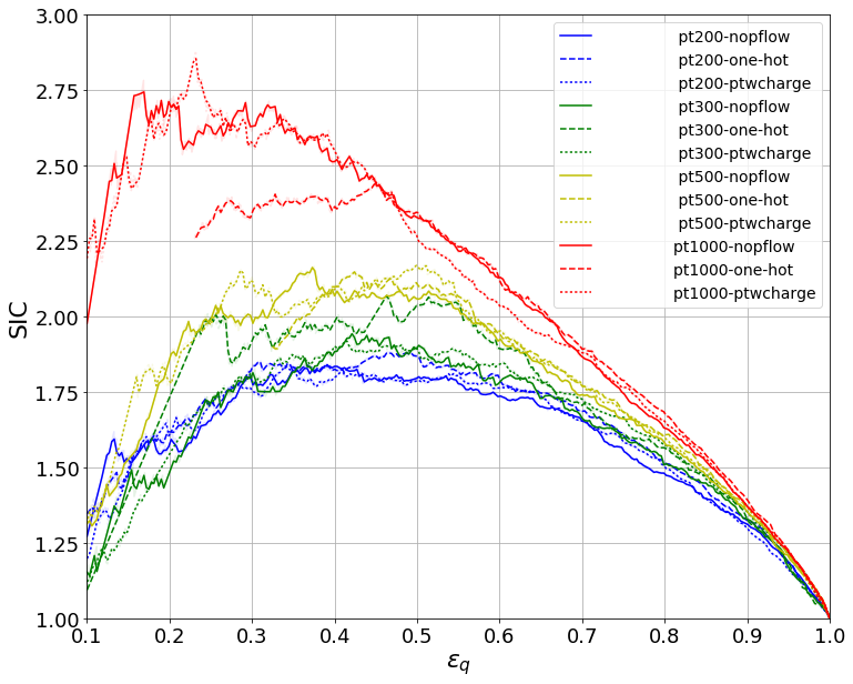
To see the $p_{T}$ dependence, we show the ROC curves of RecNN for different bins of jet $p_{T}$ in Fig. 6. Different from Fig. 5, here we are showing the (1/$\epsilon_{g}$ v.s $\epsilon_{q}$) for a clear comparison. The discriminating power increases along with jet $p_{T}$, which coincides with the behavior in conventional approach, since for higher $p_{T}$, the multiplicity ratio between gluon and quark $\frac{N_{g}}{N_{q}}\sim\frac{C_{A}}{C_{F}}=\frac{9}{4}$ increases and slowly reaches its asymptotic limit. The SICs are shown in Fig. 7.

For a detailed tabulation of results in numbers, one can find the AUCs and background rejection rates for different $p_{T}$s in Table 2. Here the rejection rate is defined as $R_{\epsilon_{S}}=1/\epsilon_{B}~{}@~{}\epsilon_{S}$.

ROC AUC $\mid$ $R_{\epsilon=80\%}$ $\mid$ $R_{\epsilon=50\%}$	200 GeV	300 GeV	500 GeV	1000 GeV
BDT	0.8164 $\mid$ 3.1 $\mid$ 10.5	0.8443 $\mid$ 3.8 $\mid$ 16.5	0.8385 $\mid$ 3.5 $\mid$ 14.1	0.8421 $\mid$ 3.6 $\mid$ 16.1
RecNN without pflow identification	0.8344 $\mid$ 3.4 $\mid$ 12.9	0.8390 $\mid$ 3.6 $\mid$ 14.4	0.8505 $\mid$ 3.9 $\mid$ 16.9	0.8623 $\mid$ 4.2 $\mid$ 21.9
RecNN with categorical pflow	0.8392 $\mid$ 3.6 $\mid$ 14.0	0.8443 $\mid$ 3.8 $\mid$ 16.5	0.8517 $\mid$ 4.0 $\mid$ 17.8	0.8637 $\mid$ 4.4 $\mid$ 22.0
RecNN with pt-weighted charge	0.8340 $\mid$ 3.5 $\mid$ 12.8	0.8453 $\mid$ 3.9 $\mid$ 14.5	0.8525 $\mid$ 4.0 $\mid$ 18.6	0.8616 $\mid$ 4.3 $\mid$ 20.4

Table 2: AUCs and background rejection rates for different jet $p_{T}s$. The baseline BDT and three scenarios concerning particle flow identification are considered. The largest AUCs and $R_{\epsilon=50\%}$s are highlighted in bold.

Variants in Network Details and Jet Clustering

In order to find out how the performance is affected by relevant factors, several variants of the procedure are examined. For simplicity, the experiments are only carried with samples of $p_{T}=200$ GeV. The results are shown in Table. 3.

• Cone size: larger cone size of jet clustering of 0.7 is examined.

• Dismissing the self-representation $u_{k}$ for embedding (since all the information is already contained by the children) in Eqn. 3, i.e. Eqn. 12. Thus the number of embedding parameters is reduced almost by 1/3 with $W_{h}\in\mathcal{R}^{q*3q}\to W_{h}\in\mathcal{R}^{q*2q}$. Not much difference is found for the performance, which means one can even reduce the size of the model while maintaining the performance.

  $$\textbf{h}_{k}=\sigma\left(W_{h}\left[\begin{array}[]{c}\textbf{h}^{\rm jet}_{k_{L}}\\ \textbf{h}^{\rm jet}_{k_{R}}\end{array}\right]+b_{h}\right)$$ (12)

• Different input feature sets are tested. The default input feature vector is ${\bf x}_{i}=(p_{i},\eta_{i},\phi_{i},E_{i},E_{i}/E_{J},p_{Ti},\theta_{i}=2\arctan(\exp(-\eta_{i})))$. And here other possibilities are experimented: ($p_{T}$, $\eta$, $\phi$); ($\eta$, $\phi$); ($p_{T}$); and only particle flow identification (either one-hot implementation (“only one-hot”) or recursively defined pt-weighted charge). One can find in Table 3 that for all the sets we have tried, $R_{\epsilon=50\%}$ can at least reach 11.3 (i.e. mis-identification rate is 8.8%). What is intriguing, only particle flow information without any other information from the momentum or angular location already gives us a fairly good result. This again corresponds to the dominance of constituents count. There might be redundant information in the full set.

• Multiparton Interaction (MPI): we examined the effects of MPI, and no significant difference was observed.

Variants	AUC	$R_{\epsilon=50\%}$
Baseline	0.8344	12.9
R=0.7	0.8210	12.4
$W_{h}\to R^{q\times 2q}$	0.8268	12.3
$W_{h}\to R^{q\times 2q}$ with one-hot	0.8313	13.7
x=($p_{T}$, $\eta$, $\phi$)	0.8291	11.8
x=($\eta$, $\phi$)	0.8249	11.9
x=($p_{T}$)	0.8264	11.6
only one-hot	0.8255	11.9
x=($Q^{\rm rec}_{\kappa=50\%}$)	0.8234	11.3

Table 3: Comparison of variants in the network settings. Here ”Baseline” is the original RecNN without pflow in Table. 2.

These experiments have shown that in the case of q/g discrimination, RecNN is quite robust against the variances in input features. And there is still large space for even simplifying the model. This is partially due to the fact that in q/g tagging the discrete particle count already dominates, thus most of the information is already contained in the tree structure itself.

3.2 (Light) Quark Jet Flavor

As a bonus, we also checked the RecNN performance on a more difficult task: light quark flavor identification. Since for all the light quarks, the dominant QCD effects are universal. And also no heavy-flavor final states, which can have long enough life time such that leave secondary vertices at the detector, are present. A possible discriminating element would be remnant electric charge, although the main effects might be washed out by parton show and hadronization. However it’s been shown Krohn:2012fg that even at the LHC, there is still a great potential for measuring jet electric charge. In Fig. 8, we show the distributions of pt-weighted jet charge ($\kappa=0.5$) for u-quark initiating jets and d-quark initiating jets with $p_{T}=1$ TeV.

Jet charge as a useful tool to identify initiating light quark flavor has been measured at the LHC Sirunyan:2017tyr ; Aad:2015cua . And it’s obviously promising if we can proceed further in this direction.

Figure 8: Distributions of pt-weighted jet charge ($\kappa=0.5$) for jets initiating from u-quark and d-quark with $p_{T}=1$ TeV.

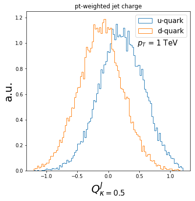
We take u/d discrimination as an attempt. Jets corresponding to u and d partons are sampled from the production processes of scaled-up W and Z bosons, at the 13 TeV LHC: $pp\to W^{\prime}/Z^{\prime}\to q\bar{q}$. Reconstructed jets are matched to the initiating partons by the criterion of $\Delta R<0.5$ between the center of jet and the parton. The network architecture and the training settings are similar to the ones in Subsection 3.1.

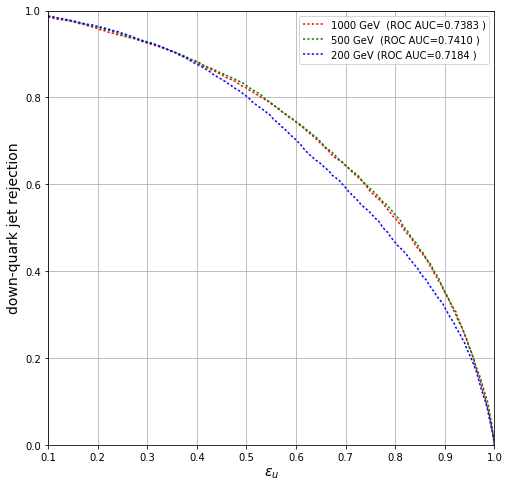
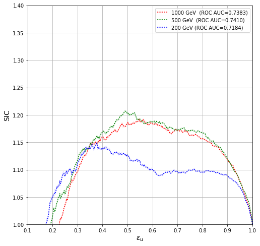
Results are shown in Fig. 9 and Table 4. The RecNN without particle flow and RecNN with the one-hot implementation are not showing any discriminating power. Only the hybrid version with pt-weighted charge carried in the embedding is behaving. We also examined several variants: using only tracks; using tracks and photons. The results showed that using only tracks is enough. A comparison is made between the single observable pt-weighted jet charge and RecNN. This hybrid implementation gives matching performance to the pt-weighted charge.

This small experiment shows although no significant improvements respect to the original observable of jet pt-weighted charge, but it can be useful for a larger framework for multi-class classification in jet flavors (gluon, b-tagging, c-tagging, light flavor identification). And it also might be useful for boosted W/Z jet tagging.

Figure 9: On the left panel, ROCs of RecNNs are shown for u/d discrimination; on the right hand side, corresponding SICs are shown. Benchmark $p_{T}$s include 200 GeV, 500 GeV and 1 TeV.

ROC AUC $\mid$ $R_{\epsilon}=50\%$	200 GeV	500 GeV	1000 GeV
$Q_{\kappa=0.5}$	0.7317 $\mid$ 5.3	0.7487 $\mid$ 5.9	0.7437 $\mid$ 5.7
RecNN with pt-weighted charge	0.7184 $\mid$ 5.1	0.7410 $\mid$ 5.8	0.7383 $\mid$ 5.6

Table 4: Discriminating u/d quark with pt-weighted charge information implemented in RecNN. The traditional single pt-weighted charge ($Q_{\kappa=0.5}$) is used as baseline.

4 Conclusions

In Ref. Louppe:2017ipp , the framework of RecNNs for jet physics is built and for the first time tested on W/QCD tagging. Motivated by the advantages of efficiency and nice structure of RecNN, and the previous findings on its capability, we in this work try to further explore its application in an advanced topic for jet physics at the LHC: quark/gluon discrimination. And in order to make use of all the information collected at the detectors, we also explored the implementation of particle flow in RecNN. Besides, some variants for the network details are examined in Section 3.1 to figure out the relevant factors. Moreover, a first attempt to identify jet electric charge was made in Section 3.2 , using recursively embedded pt-weighted charge. These results show a great potential for RecNNs in broader application and in realistic use.

In the RecNN approach, the raw data taken from detectors are fed into the networks directly without information loss. By embedding the jet data through a tree-like recursive process and subsequently feeding into following classifier, one has a natural and efficient DNN strategy for jet tagging. We first investigated the performance of RecNN on pythia-level data, i.e. the hadrons without detector effects. Then we employed fast detector simulation and took the detector measurements as input. At this stage, RecNNs can give discrimination power of rejecting $\sim$95% gluon jets at $\epsilon_{q}=50\%$ for $p_{T}=1$ TeV. As for extra particle flow identification implemented in RecNNs, slight increase can be generally observed (especially for lower jet $p_{T}$s), but not significant enough. We examined several variants on the details of the procedure, and interestingly the results showed that even only with particle flow identification, RecNNs still give fairly good performance. This might indicate that most of the information for q/g discrimination is already contained in the tree-structure itself. Pile up effects are not taken into account in this work, and jet grooming is also not examined here. These can be left for future work.

As a byproduct, we also apply the RecNN with recursively defined charge to a more difficult task in jet physics: jet flavor (light quarks) identification. It actually is the simplest extension from the conventional pt-weighted jet charge to its DNN version. And it’s showing no better performance, but still gives the discrimination power at the same level. We hope it will help in further study on multi-class classification in jet physics.

Thus as conclusions, we have:

• The results with detector simulation indicate a great potential for RecNN in q/g discrimination.

• RecNN is robust against the variances in input feature sets. The tree structure itself already contains most of the information in q/g discrimination. This is partly due to the fact that the particle multiplicity dominates in q/g tagging.

• Extra particle flow identification is not showing significant effects in q/g discrimination, indicating the saturation of input information here.

5 Discussion and Outlook

There are several interesting aspects and extensions which deserve further investigation. Here we briefly discuss on a few of them.

Event Level Analysis

Actually a jet can’t be isolated from the remnants of the event, although we can get quite “pure” jets by grooming. Color connections can be very useful in many cases. How to manifest these effects also deserves attention. And it might be potential if we can deal with them better in event-level analysis.

Easy to be extended to event-level analysis is an important motivation for RecNN. It is natural to be augmented into lager hierarchical structure. The event analysis with only jets has been explored in Louppe:2017ipp . A simple RNN chain is used there for constructing events from jets. About the implementation in event-level, how to structure the whole event is not trivial. Every event can be seen as a structured data tree, and the whole information of one event just reside within the properties of the nodes and links between these nodes. How to properly represent every object and its connections with other parts of the event would be crucial for designing NN architectures.

Jet Algorithms as Unsupervised Learning Procedure

In the framework of DNN, accordingly adjusting the jet clustering might help to gain better performance. Actually jet finding itself can be treated as a minimization problem Angelini:2004ac ; Grigoriev:2003yc ; Grigoriev:2003tn ; Volobouev:2009rv , thus it will be very interesting if we can naturally include the process of jet finding in event-level implementation.

Application: New Physics

Generally speaking, new physics will have interesting patterns when concerned with their new particle spectrum and decay modes. For example, SUSY events will generally produce large amounts of final states (more complicated hierarchical structure), and sometimes several soft leptons in electroweakino search. Whether DNNs have better tolerance on this kind of topologies is also worthwhile for investigation.