Lisco: A Continuous Approach in LiDAR Point-cloud Clustering

Abstract

The light detection and ranging (LiDAR) technology allows to sense surrounding objects with fine-grained resolution in a large areas. Their data (aka point clouds), generated continuously at very high rates, can provide information to support automated functionality in cyberphysical systems. Clustering of point clouds is a key problem to extract this type of information. Methods for solving the problem in a continuous fashion can facilitate improved processing in e.g. fog architectures, allowing continuous, streaming processing of data close to the sources. We propose Lisco, a single-pass continuous Euclidean-distance-based clustering of LiDAR point clouds, that maximizes the granularity of the data processing pipeline. Besides its algorithmic analysis, we provide a thorough experimental evaluation and highlight its up to 3x improvements and its scalability benefits compared to the baseline, using both real-world datasets as well as synthetic ones to fully explore the worst-cases.

I Introduction

Active sensors that are able to measure properties of the surrounding environment with very fine-grained time resolution are utilized more and more in cyber-physical systems, such as autonomous vehicles, digitalized automated industrial environments and more. These sensors can produce large streams of readings, with the LiDAR (light detection and ranging) sensor being a prominent example. A LiDAR sensor commonly mounts several lasers on a rotating column; at each rotation step, these lasers shoot light rays and, based on the time the reflected rays take to reach back the sensor, they produce a stream of distance readings at high rates, in the realm of million of readings per second.

As common in big data applications, one of the challenges in leveraging the information carried by such large streams is the need for efficient methods that can rapidly distill the valuable information from the raw measurements [8, 5, 17, 28]. A common problem in the analysis of the LiDAR sensor data is clustering of the raw distance measurements, in order to detect objects surrounding the sensor [22]. This can, for instance, enable the detection of surrounding obstacles and prevent accidents (e.g. avoiding pedestrians in autonomous driving) or study the motion feasibility of objects in factories’ production paths [1].

Challenges and contributions

The processing time incurred by clustering of raw measurements (aka point clouds) represents one of the main challenges in this context because of the high rates and the need for the clustering outcome to be available in a timely manner for it to be useful. Furthermore, the accuracy of the clustering is challenging as well, since readings from objects that are at different distances from the sensor can vary a lot in density.

A key performance enabler for high-rate data streaming analysis is the pipelining of its composing tasks. Nevertheless, common state-of-the art approaches for clustering of LiDAR data (cf [27],[21],[24] and more detail in § VII elaborating on related work) first organize the points to be clustered (e.g. sorting them so that points close in space are also close in the data structure maintaining them) and only then perform the clustering by querying the organized data (e.g. by running neighbor-query as discussed in § II). By doing this, they introduce a batch based processing that affects the clustering performance.

To overcome this, we target a single-pass analysis that will enable fine-grained pipelining in processing the data. We propose a new method that achieves LiDAR data-point clustering, called Lisco, that allows to boost processing throughput by maximizing the internal pipelining of the analysis steps, through a key idea that can exploit the inner ordering of the data generated by a LiDAR sensor.

In more detail, we make the following contributions:

1. We introduce Lisco, a new algorithm for Euclidean-distance-based clustering of LiDAR point clouds, that maximizes the granularity of the data processing pipeline, without the need for supporting sorting data structures.

2. We provide a fully implemented prototype and we discuss Lisco’s complexity in connection to the state-of-the-art Euclidean-distance-based clustering method in the Point Cloud Library (PCL), which we adopt as baseline due to its known accuracy, efficiency and wide use-base [22].

3. We perform a thorough comparative evaluation, using both real-world datasets as well as synthetic ones to fully explore the worst-cases and the spectrum of trade-offs. We achieve a significant improvement, up to 3 times faster than the baseline and we also show significant scalability benefits.

The rest of the paper is organized as follows. § II overviews the LiDAR sensor, the data it produces and clustering-related techniques that exist for such data. § III presents the main idea, the outline and argues about the properties of the proposed Lisco method, while the algorithmic implementation is given in § IV. We evaluate the proposed method in § VI. Finally, we discuss related work and conclude in § VII and § VIII, respectively.

II Preliminaries

In this section, we give details about the key properties of LiDAR sensors and the data they generate. We also provide a detailed problem description and evaluation criteria of solutions. Finally, we briefly describe the Euclidean-distance based clustering method in PCL, which we use as baseline as explained in the introduction.

II-A LiDAR - sensor and data

The light detection and ranging (LiDAR) technology allows sensing surrounding objects with fine-grained resolution in a large areas.

The LiDAR sensor mounts $L$ lasers in a column, each measuring the distance from the target by means of the time difference from emitted and reflected light pulses. The column of lasers performs $R$ rotations per second, each consisting of $S$ steps, producing a set of $n$ points, also called point cloud. The number of points reported by the LiDAR sensor for each rotation can be lower than $L\times S$, since some of the emitted pulses might not hit any obstacle. We refer to the angle in the x-y plane between two consecutive steps as $\Delta\alpha$ (e.g. measured in radians) and to the elevation angle from the x-y plane between two consecutive lasers as $\Delta\theta$. Each point $p$ is described through attributes $\left<d,l,s\right>$ where $d$, $l$, $s$ are the measured distance, the laser index and the step index. The measured distance, $d$, is a value greater than or equal to 0. Value 0 for $d$ shows no reflection in the point. In the following, we use the notation $p_{x}$ to refer to attribute $x$ of point $p$ (i.e., $p_{d}$ refers to the distance reported for point $p$).

Figure 1: Top and side views for the LiDAR’s emitted light pulses showing steps and lasers, together with the resulting 2D view. In the 2D view, non-reflected pulses are white while reflected ones are coloured.

Let us consider in the following examples that $L=8$ and $S=8$. We visually present the points by unfolding them as a 2D matrix, where each column contains $L$ rows and each rotation step is a column. We assume that new data is delivered from the physical sensor with the granularity of one rotation step (Figure 1).

II-B Problem formulation: from point clouds to clusters

Given a set of points corresponding to LiDAR measurements, we want to identify disjoint groups of them that can be potential objects in the environment surrounding the sensor. A natural criterion, commonly used in the literature and applications, is the distance between points. In particular, adopting the problem definition in [20] (Chapter 4), which we paraphrase here for ease of reference:

Definition 1.

[Euclidean-distance based clustering] Given $n$ points in 3D space, we seek to partition them into some (unknown) number of clusters $C$ using the Euclidean-distance metric, such that every cluster contains at least a predefined number of points ($minPts$), that is $\forall j,|C_{j}|\geq minPts$, and all clusters are disjoint, that is $C_{i}\cap C_{j}=\emptyset,\forall i\neq j$. Two points $p_{i}$ and $p_{j}$ should be clustered together if their Euclidean distance $||p_{i}-p_{j}||_{2}$ is at most $\epsilon$, with $\epsilon$ being a predefined threshold.

To facilitate the presentation of the baseline algorithm and our proposed one, we introduce the $\epsilon$-neighborhood of a point $p$: the set of points of the input whose Euclidean distance from $p$ is at most $\epsilon$. A set of points closed under the union of their $\epsilon$-neighborhoods is characterized as noise if its cardinality is less than $minPts$.

It should be noticed that, when clustering data from scenarios like the vehicular one, a pre-processing task is usually defined to filter out points that refer to the ground, since many objects laying on it would be otherwise clustered together. Since ground removal can be implemented as a non expensive and continuous filtering operation [10] (e.g. by removing points below a certain threshold, as we do in § VI) we do not further discuss it in the remainder.

II-C Euclidean-distance based clustering in PCL

PCL [22] provides a set of tools based on a collection of state-of-the-art algorithms to process 3D data, including filtering, clustering, surface reconstruction and more. In this section we review its method for cluster extraction, which is an Euclidean-distance based clustering and we use it as a baseline. For brevity we call this algorithm PCL_E_Cluster in the rest of this document.

PCL_E_Cluster works on batches of data points. It first builds a kd-tree to facilitate finding the nearest neighbors of points. Subsequently, it proceeds as described by algorithm 1 to extract the clusters.

Algorithm 1 Main loop of PCL_E_Cluster

1:clusters = $\emptyset$

2:for $p\in$ P do

3:    Q = $\emptyset$

4:    if $p$.status $\neq$ processed then

5:         Q.add($p$)

6:         for $q\in$ Q do

7:             $q$.status = ’processed’

8:             $N$ = GetNeighbors($q,\epsilon$)

9:             Q.addAll($N$)          

10:         if $\text{size(Q)}\geq\text{{minPts}{}}$ then clusters.add(Q)              

Starting from any arbitrary unprocessed point $p$, the algorithm adds it in an empty list, $Q$ (line 5). Then, PCL_E_Cluster adds all the points of the $\epsilon$-neighborhood of each member of Q to it. After processing all members of the list $Q$, if its size is greater than or equal to minPts, the list is returned a cluster. The algorithm continues with the next unprocessed point, to explore another cluster. The procedure is terminated when all input points have been processed. We discuss the computational complexity of algorithm 1 in § V.

III Lisco

We present in this section Lisco. We first discuss the intuition behind the algorithm, i.e. a continuous, single-pass approach in clustering in contrast to existing batch based methods as discussed in § II. Subsequently, we focus on the challenges and trade-offs that continuous clustering introduces.

III-A Towards continuous clustering

Based on the clustering requirements as introduced in Definition 1, each point $p$ reported by the LiDAR sensor is temporarily clustered with each neighbor point $p^{\prime}$ within distance $\epsilon$ from $p$. A cluster of points is eventually delivered if it contains at least minPts points, otherwise its points are characterized as noise. As discussed in § II-C, implementations such as the one provided by PCL limit the pipelining of the analysis because of processing stages that cannot be executed concurrently. More concretely, they first traverse all the points to populate a supporting data structure that facilitates finding the points in the $\epsilon$-neighborhood of each point $p$ (a kd-tree in the case of PCL) and subsequently they traverse a second time all the points to cluster them.

Figure 2: Top and side views (A and B) showing which steps and lasers, respectively, to include in the neighbor mask (C) for the latter to contain at least all the points within distance $\epsilon$ from $p$.

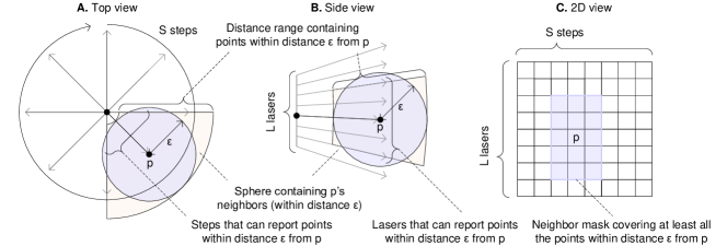
As shown in Figure 2, the intuition behind Lisco is that the search space for the $\epsilon$-neighborhood of point $p$ can be translated into a set of readings given by certain steps (Figure  2.A) and lasers (Figure  2.B) around $p$, and within a certain distance range from the LiDAR’s emitting sensors. It should be noted that these constraints describe a region of space that may also contain points whose distance from $p$ is greater than $\epsilon$. Nevertheless, if points within distance $\epsilon$ from $p$ exist, they will be returned by one of these steps and lasers and will fall within the given distance range, as we further explain in § V.

Thus, in order to discover the $\epsilon$-neighborhood of point $p$, by leveraging the sorted delivering of tuples from the LiDAR sensor step after step, it is enough to explore a neighbor mask centered in $p$, as shown in Figure 2.C. In this way, we eliminate the need for a search-optimized data structure like kd-trees, and we allow the algorithm to process data as they are received from the sensor.

III-B Coping with the challenges of continuous clustering

The continuous one-pass analysis of Lisco introduces several challenges that are not found in batch based approaches. Here we discuss and explain how they are addressed in Lisco in the following.

III-B1 Partial view of neighbor mask

Algorithm 2 shows how the neighbor mask is computed, i.e. the number of previous and subsequent steps $\sigma$ and the number of upper and lower lasers $\lambda$ that possibly contain points within distance $\epsilon$ from $p$. As discussed in § II, $\Delta\alpha$ and $\Delta\theta$ refer to the minimum angle differences between two consecutive steps and lasers, respectively.

Algorithm 2 Given point $p$, compute the number of previous steps $\sigma$ and upper and lower lasers $\lambda$ bounding at least all the points within distance $\epsilon$ from $p$.

1:procedure getNeighborMask($p$)

2:    $\lambda\leftarrow\lceil|\arcsin(\epsilon/p_{d})|/\Delta\theta\rceil$

3:    $\sigma\leftarrow\lceil|\arcsin(\epsilon/p_{d})|/\Delta\alpha\rceil$

4:    return $\lambda,\sigma$

Algorithm 3 Main loop of Lisco

1:$subclusters$ = $\emptyset$

2:upon event reception of step $s$ do

3:    for $l\in{1,\ldots,L}$ do

4:         $p$ = $M[l,s]$

5:         if $p_{d}>0$ then

6:             $\lambda,\sigma$ = getNeighborMask($p$)

7:             cluster($p$,$\sigma$,$\lambda$,$subclusters$)              

8:upon event all steps processed do

9:    for $subcluster$ $\in$ $subclusters$ do

10:         if size($subcluster$) $\geq\text{{minPts}{}}$ then return $subcluster$              

The main loop of Lisco, Algorithm 3, processes points in $M$, the 2D matrix of input points (described in § II), in step and laser order (Line 4). Each point is processed only if its distance is greater than 0 (that is, if the LiDAR’s pulse has been reflected for the point’s step and laser index) (Line 5). Once all the points have been processed, all the clusters containing at least minPts points are delivered. As it can be noticed, the parameter minPts does not have an effect in the complexity of the algorithm, since it is only used to filter the delivered clusters at the very end of the clustering process. We describe how clusters are discovered and managed within the function cluster in the following.

Given points $p_{1}$ and $p_{2}$ within distance $\epsilon$, $p_{1}$’s neighbor mask will contain $p_{2}$ and vice versa. To avoid comparing each pair of neighboring points twice, it is enough to consistently traverse half the neighbor mask. Lisco explores the half containing the $\lambda$ lasers above and below $p$ and the $\sigma$ steps on $p$’s left side. This allows for points in $p$’s step to be processed as soon as they are delivered (points on $p$’s right side are yet to be delivered upon reception of $p$’s step points). Take into account that, for a minority of steps, not all the points on $p$’s left side lay on columns with a lower index than $p$’s (i.e., they are not stored on the left side of the $M$ matrix). For instance, if a point in column 2 should be compared with 3 columns on the left ($\lambda=3$), then it should be compared with columns S-1, S and 1. In such a case, some comparisons must be postponed until such steps are delivered. A point $p^{\prime}$ on the left side of $p$ and within distance $\epsilon$ lays on a lower index than $p$ if $0\leq p_{s}-p^{\prime}_{s}\leq\sigma$. On the other hand, if $p^{\prime}_{s}+\sigma>S$, then $p^{\prime}$ is on the left side and within distance $\epsilon$ from points in steps $1,\ldots,p_{s}+\sigma-S$. In both cases, the clustering semantics defined in § II require $p$ and $p^{\prime}$ to be compared, as we do in Algorithm 4.

III-B2 Continuous cluster management

A second challenge brought by the continuous nature of Lisco is that subclusters evolve as more steps arrive. Hence, a cluster identified once all the points in a rotation are processed might be the union of several previously discovered subclusters, as seen in Figure 3. Figure 3.A shows the subclusters found when half of the points in the rotation have been processed. In the example, 5 points have been clustered in $C_{1}$ and 4 points have been clustered in $C_{2}$. The other non-colored points have not been clustered since they had no neighbors within distance $\epsilon$. Figure 3.B shows the clusters found when all the points in the rotation have been processed. At this stage, the points previously clustered in different subclusters are now clustered together. The point marked with $x$ represents the point that has one neighbor in each of the two disjoint subclusters found by Lisco. Once $x$ is processed, these two subclusters should be merged.

Figure 3: Example showing how the points of two subclusters, that evolve concurrently in Lisco’s continuous analysis, may end up in the same cluster at a subsequent step.

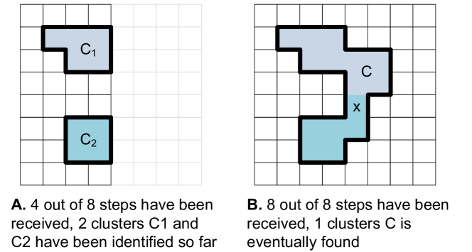
Based on this observation, we introduce the following informal notions to facilitate the detailed description of Lisco. A subcluster is a set of points that have been clustered together during the processing of the previously received steps of the input. A cluster is a set of at least minPts points that have been clustered together once all the steps of the input have been processed, i.e. a subcluster with cardinality at least minPts is characterized as a cluster after all the steps have been processed. Finally, we consider each subcluster to have a unique identifier called head.

Based on the above, one can notice that a subcluster can contain points that previously belonged to two or more subclusters. Because subclusters are found continuously while the points of a rotation are being processed, the clustering algorithm requires methods to: (1) retrieve the head of the points belonging to a subcluster and (2) merge two subclusters together in order for the final cluster to be delivered as a single item. In order to do this, we use in Algorithm 4 (overviewing the clustering process applied to each incoming point $p$) the functions Head $H$ = getH(Point $p$) and merge(Head $H1$,Head $H2$). Once two subclusters are merged invoking function merge, we expect the function getH to return the same head for any point of the two subclusters. Without loss of generality, we assume this head to be $H_{1}$ in the following. Because of this we define a third function setH(point $p$,Head $H$). Finally, we define the function createH() to allow for newly discovered subclusters to be instantiated.

Algorithm 4 Given point $p$, cluster it together with all the points already received from the LiDAR sensor that are within distance $\epsilon$ from it.

1:procedure cluster($p$,$\lambda$,$\sigma$,$subclusters$)

2:    for $p^{\prime}|(0\leq p_{s}-p^{\prime}_{s}\leq\sigma\vee 1\leq p^{\prime}_{s}\leq p_{s}+\sigma-S)\wedge\left|p_{l}-p^{\prime}_{l}\right|\leq\lambda\wedge\left|p_{d}-p^{\prime}_{d}\right|\leq\epsilon$ do

3:         $H_{1}$=getH(p)

4:         $H_{2}$=getH(p’)

5:         if $H_{1}\neq H_{2}\wedge||p-p^{\prime}||_{2}\leq\epsilon$ then

6:             if $H_{1}=\emptyset\wedge H_{2}=\emptyset$ then

7:                 $H$ = createH()

8:                 setH($p$,$H$)

9:                 setH($p^{\prime}$,$H$)

10:                 $subclusters$.add($H$)

11:             else if $H_{1}=\emptyset\wedge H_{2}\neq\emptyset$ then

12:                 setH($p$,$H_{2}$)

13:             else if $H_{1}\neq\emptyset\wedge H_{2}=\emptyset$ then

14:                 setH($p^{\prime}$,$H_{1}$)

15:             else

16:                 $subclusters$.remove($H_{2}$)

17:                 merge($H_{1}$,$H_{2}$))                           

As shown in Algorithm 4, four different cases should be checked for two points within distance $\epsilon$ that do not belong to the same subcluster:

• Line 6: None of the two points belongs to a subcluster. In this case, a new subcluster head is created and set for both points

• Line 11: Point $p$ does not belong to a subcluster while point $p^{\prime}$ does. In such a case, point $p$ will refer to the same head as point $p^{\prime}$.

• Line 13: Point $p$ belongs to a subcluster while point $p^{\prime}$ does not. In such a case, point $p^{\prime}$ will refer to the same head as point $p$.

• Line 15: Both points $p$ and $p^{\prime}$ have been clustered but to different subclusters. In such a case these two subclusters are merged together.

IV Algorithmic implementation

We discuss the details of the algorithmic implementation of Lisco in this section.

Data points are kept in a 2D matrix, $M$. The number of rows and columns in the matrix is equal to the number of lasers and steps respectively. Upon reception of a column of points from LiDAR, which contains the reflected points of all lasers in one step, we store them in the corresponding column of the matrix. By using the laser and the step number, all the attributes of a point can be extracted in constant time. Each entry in $M$ holds the attributes of the corresponding point and a pointer (initially set to NULL) to the head of its subcluster. The head of a subcluster is defined as the point with the lowest indices in lexicographical order of steps and lasers during the creation of a new subcluster. When two subclusters are merged, the head from the subcluster with the largest number of members is maintained.

$Subclusters$ is a hash map used in order to keep track of subclusters and their corresponding members. It is implemented as a linked list of arrays, where each key is the header of a subcluster and its members are stored in the array. If the size of a subcluster exceeds the size of the array, a new array is linked to the tail of the current array, so that subclusters can grow without restriction. At the end of the clustering procedure, we use $subclusters$ to traverse through subcluster heads. Each subcluster that has more than minPts members is announced as a cluster, otherwise it is characterized as noise.

To keep of Lisco’s time complexity low (discussed in § V) we aim at efficient time complexity of the main methods used in our algorithms. As shown in Algorithm 2, function getNeighborMask is executed in constant number of steps, since it boils down to a fixed number of numerical operations. Similarly, functions createH and setH can be also implemented to incur in $O(1)$ complexity, as we discuss in the following. The algorithmic implementation of getH and merge induces the following trade-off. On the one hand, merge can be implemented to induce $O(1)$ time-cost; this can be done by maintaining a hierarchy of subclusters being part of the same subcluster while incurring a higher cost for the getH, linear in the number of subclusters. Figure 4 shows how some of the points clustered together once all the data is processed point to head $H_{1}$ via head $H_{2}$. For these points the getH method has a cost higher than that of the points directly pointing to $H_{1}$, which depends on the chains induced by the data structure to maintain the hierarchy. In the proposed implementation we opt for an $O(1)$ cost for method getH and a higher cost for merge, as seen in Figure 5 and § V. The reason, as can be seen in Algorithm 4 and based also on our empirical evaluation in § VI, is that getH is executed twice for pairs of points being compared, while merge is executed significantly less often.

Figure 4: Possible implementation in which the merge method is made $O(1)$ by hierarchically linking heads of subclusters belonging to the same subcluster. Notice that the complexity of getH is no longer $O(1)$ but linear in the number of subclusters for some of the points.

Figure 5: Possible implementation in which the getH method can run in $O(1)$ steps by having all points directly linked with the subcluster head. Notice the head of all the points of subcluster $C_{2}$ has been updated when the subcluster has been merged with subcluster $C_{1}$.

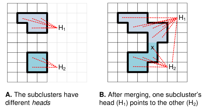
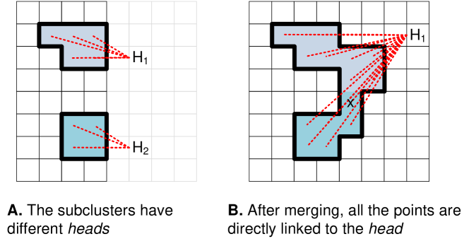
In detail, the implementations of the functions used in Algorithm 4 are as follows:
- createH: This function gets two points that do not belong to any subcluster, and returns the one with the lower index-pair for step and laser. Since the returned point will be head of a subcluster, a new node is created in the $subclusters$ and the head is mapped to it.
- setH: This function sets the pointer of a point to the head point. By calling this function, we are adding a point to a subcluster with an identified head. The point also needs to be added as the last element in the array of the mapped head.
- getH: This function reads the pointer to get the head point. If two points are in the same subcluster, they get the same head point as the result of this function.
- merge: If two points belong to different subclusters, Lisco merges the two subclusters by calling this function. It chooses the subcluster with bigger number of members as the base subcluster, and merges the other one by changing the head of its members to the base subcluster’s head. After merging subclusters, it is also necessary to remove the merged subcluster’s head from the $subclusters$ hash map and append its array to the base subcluster’s array.

V Analysis

V-A Correctness

Based on Lisco’s functionality and algorithmic implementation, we discuss here why Lisco’s outcome satisfies Definition 1.

Claim 1.

If two points $p$ and $p^{\prime}$ are in the $\epsilon$-neighborhood of each other they will either be in the same cluster at the end of Lisco procedure or be characterized as noise, in the same way as given in Definition 1.

Proof.

(sketch) Consider that, w.l.o.g. $p$ is processed second. As argued in paragraph getNeighborMask in the previous section, $p^{\prime}$ will be found that it belongs in the $\epsilon$-neighborhood of $p$. This implies that they will be merged/inserted in the same subcluster. Unless that subcluster in the end is found to contain fewer points than $MinPts$, it will be return as a final cluster in the end of the main loop of Lisco. ∎

V-B Complexity

In this section, we discuss the complexity analysis of Lisco and compare it with PCL_E_Cluster.

Regarding PCL_E_Cluster, the required processing work volume is similar to the DBSCAN algorithm, i.e. building a spatial index (kd-tree) and using it to execute region queries for each point, resulting in an overall expected time complexity of $O(nlogn)$ processing steps [25, 4, 19].

Claim 2.

Lisco’s time complexity is linear in the number of points, multiplied by a factor that depends on the size of the clusters in the set of data points. In the worst-case where there is a big cluster of $O(n)$ points, it can take $O(nlogn)$ processing steps for Lisco to complete.

Proof.

(sketch) Overall, the time complexity of Lisco is the number of iterations in the main loop (i.e. $n$, as the number of points), times the work in each iteration, i.e. for each point (i) finding its $\epsilon$-neighborhood, and (ii) working with each point in the neighborhood.

Part (i) from above, induces an asymptotically constant cost, depending on $\epsilon$, as it is performed through the comparisons implied by the masking operation getNeighborMask. Part of the $\epsilon$-neighborhood of a point $p$, i.e. the points with smaller step index, is compared with $p$ through step 2 of Algorithm 4 on behalf of $p$, while for each of the remaining points $p^{\prime}$ in p’s $\epsilon$-neighborhood, $p$ will be identified as part of the $\epsilon$-neighborhood of $p^{\prime}$ when the respective step is executed on behalf of $p^{\prime}$.

Regarding part (ii), functions’ createH and setH algorithmic implementation incurs a constant number of processing steps each, as we explain in § IV. Moreover, as explained in the aforementioned section, getH induces $O(1)$ time-cost, as a point can identify its head in $O(1)$ (e.g. with a direct link). This incurs a cost that is $O(x)$ for merge, where $x$ is the size of the smaller subcluster, since the merging itself needs to update the head for all the points of the smaller one of the subclusters being merged.

Since the merge function chooses the subcluster with the bigger number of points as the base subcluster, in the worst-case the clustering has a huge subcluster of $O(n)$ points, and an unlikely scenario for constructing it, might require Lisco to merge roughly equally-sized subclusters at each of the merge operations leading to the big subcluster – any other combination of subclusters would lead at most to an equal cost as the one described. Since halving $O(n)$ points can be made at most $O(logn)$ times, we can observe that the worst-case total number of merge-related processing steps will be dominated by a sequence of $O(nlogn)$ steps, which will be the dominating cost in the worst case complexity of Lisco. ∎

VI Evaluation

In this section, we present our experimental methodology and results of Lisco and compare them with those of PCL_E_Cluster algorithm. Since the clustering outcomes of PCL_E_Cluster and Lisco are the same, we do not need to compare the clusters and we can focus on the completion time for each approach.

VI-A Evaluation setup

To run PCL_E_Cluster we use the $EuclideanClusterExtraction$ class from PCL library, which is designed to cluster 3D point clouds and is implemented in C++. We also implemented Lisco in C++11 and compiled both of algorithms with gcc-4.8.4 using the -O3 optimization flag. All the experiments have been run on the same system running Linux with 2.00GHz Intel(R) Xeon(R) E5-2650 processor and 64GB Ram.

VI-B Data

We used both synthetic and real-world datasets. The real-world dataset has been collected from the Ford Campus dataset [18] and the synthetic ones have been generated using the Webots simulator [15]. We use synthetic datasets to explore the effect of data (e.g. different total number of points that have been collected by the LiDAR, different densities and distances of objects) on the performance of algorithms.

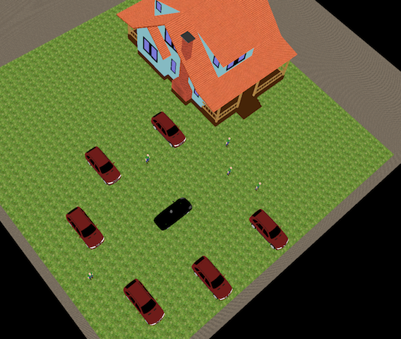
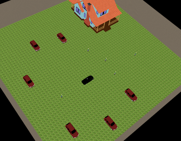
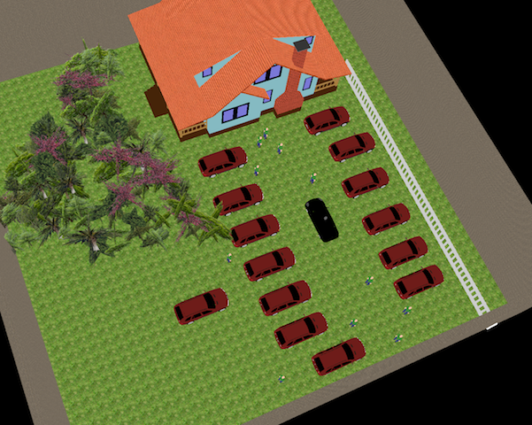
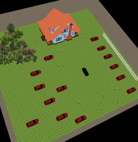
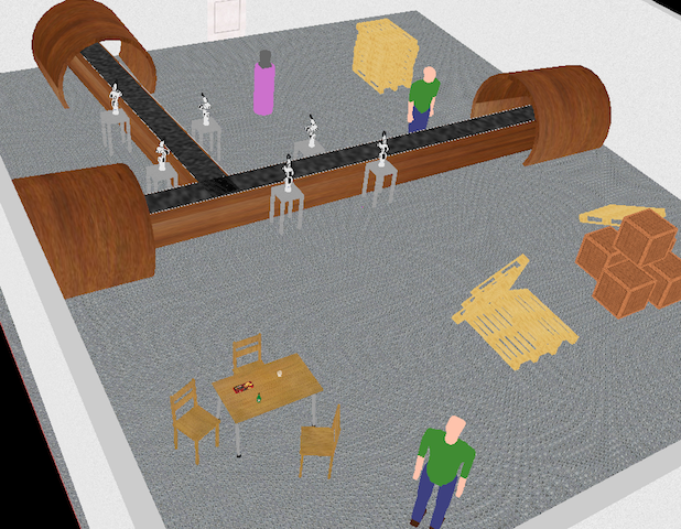
There are five scenarios for synthetic datasets. SCEN1 and SCEN2 have the same and few number of objects but we changed the position of the objects to near and far from LiDAR. Near objects reflect more points while far objects reflect fewer points with a larger gap between two nearby points. Similarly, SCEN2 and SCEN3 have the same number of objects (number of objects are more than previous scenarios) and we only changed the position of the objects. Finally, SCEN5 represents a high density environment with a lot of objects. Figure 6 shows five simulated environments for several scenarios. In all the environments, a VelodyneHDL64E is used to collect data points and generate a dataset within one physical rotation.

Table I summarizes the properties of the synthetic datasets. Since we used the same specifications for the LiDAR in all scenarios, the number of steps and lasers for one physical rotation is the same, so the total number of points (including NULL points and ground points) is the same and it is equal to 72000. After removing the ground points and eliminating NULL points, we get a number of reflected points. As shown in the table, with the same number of objects in the environment (e.g. SCEN1 and SCEN2), if we change the position of objects to near or far, we get different numbers of reflected points.

(a) SCEN1 - The simulated sparse environment in which objects are close to the LiDAR which is located on the black car

(b) SCEN2 - The simulated sparse environment in which objects are far from the LiDAR which is located on the black car

(c) SCEN3 - The simulated dense environment in which objects are close to the LiDAR which is located on the black car

(d) SCEN4 - The simulated dense environment in which objects are far from LiDAR which is located on the black car

(e) SCEN5 - The simulated room for high density environment. The LiDAR is located on the purple column

Figure 6: Different scenarios for simulated environments.

Name	# Points after removing NULL points and ground points
SCEN1	26891
SCEN2	16218
SCEN3	39028
SCEN4	18229
SCEN5	64518

TABLE I: Properties of synthetic datasets and the effect of number of objects and their distances from LiDAR on number of points after ground removal.

VI-C Performance evaluation

The execution time is measured from the time-instant the first data point of the dataset is received until the time instant when the clustering algorithm has processed all data points of one full physical rotation. A higher value of $\epsilon$ implies a larger $\epsilon$-neighborhood of a point, hence the clustering algorithm needs more time to search in the neighborhood.

VI-C1 Synthetic datasets

Figure 7 shows the average execution time with confidence level 99% on 20 runs with different values of $\epsilon$ and constant value of minPts = 10. Since the maximum margin of error for a confidence level 99% is small, we can not distinguish them clearly in the figure. We chose a range $[0.1-1]$ meters for $\epsilon$, so that for example if $\epsilon=0.4$, all the objects that their closest points have at least 40 centimetres distance from each other, should be detected as separated objects. While clustering with smaller values of $\epsilon$ find at least one cluster for each object, bigger values increase the probability of clustering distinct objects together. For example, with $\epsilon=1$ for SCEN3, all the cars at each side of the black car, are clustered together which leads to incorrect segmentation.

Figure 7: The average execution time on synthetic datasets with confidence level 99% over 20 runs for minPts = 10 and different values of $\epsilon$

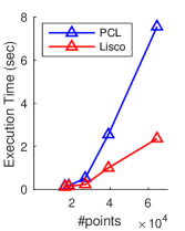
As expected, by increasing the value of the $\epsilon$, the execution time increases for both algorithms. As it can be seen, when the number of points is high, regardless of the value of the $\epsilon$, Lisco is always faster than PCL. Only for a dataset with a relatively small number of points and when $\epsilon$ is set to a high value PCL has slightly better performance than Lisco (figure 7 SCEN2 and SCEN4). The effect of number of points is also shown in figure 8. As discussed in § V building a kd-tree and using it to find nearest neighbors in PCL becomes a bottleneck when the number of points is high.

Figure 8: Scalability of Lisco and PCL with respect to the number of points

VI-C2 Real-world dataset

This Ford Campus dataset is collected by an autonomous ground vehicle testbed, with a Velodyne HDL-64E LiDAR scanner [18]. The vehicle path trajectory in this dataset contains several large and small objects (e.g. buildings, vehicles, pedestrians, vegetation, etc.). We have tested PCL_E_Cluster and Lisco on 2280 rotations of this dataset and compare their execution times with confidence level 99%.

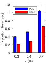
Figure 9 shows the results of the comparison for $\epsilon$ values 0.3, 0.4, and 0.7. Among all the rotations, the minimum number of reflected points after ground removal is 5000, the maximum is 75550, and the average is 50225. As shown in the figure, Lisco outperforms PCL_E_Cluster in real-world datasets. In real-world data, generally there are more objects around the LiDAR and therefore there are more reflected points besides the ground. Since Lisco processes points upon receiving them from LiDAR, it can save more time and it has thus better throughput.

Figure 9: The average execution time of running PCL and Lisco over 2280 rotations of real-world dataset for minPts = 10 and different values of $\epsilon$

VII Other related work

Data clustering has been studied for several decades and existing algorithms have been categorized into four classes: density-based, partition-based, hierarchy-based, and grid based [9]. Due to their ability in finding arbitrarily shaped clusters without requiring to know the number of the clusters a priori, density-based methods are widely used in different applications. Well-known algorithms of this class include DBSCAN [4] and OPTICS [2]. However, to use these algorithms in big data applications and overcome their performance bottleneck in dealing with extremly large datasets, there are several attempts to parallelize DBSCAN [19, 13]. In parallel models, the clustering procedure is divided into three steps: 1) data distribution (e.g. using kd-tree) 2) local clustering (which is splitted on several machines) 3) merging of local clusters. Although the efficiency is improved by splitting the clustering on several machines, pipelining of steps has not being studied yet.

Rusu et al. [21] introduce an Euclidean-distance-based clustering which is a partition-based clustering method that produces arbitrarily shaped clusters. This approach is designed for unorganized data points. So, to facilitate searching for nearest neighbors, first a kd-tree is built over the dataset and then clustering is being performed. In other works [27, 24], an octree is used to identify the neighbors before starting the clustering procedure.

Since LiDAR data points are implicitly ordered, organizing them (e.g. in a tree) may be avoided, similar to the spirit of this paper. Specifically, the characteristics of the sensor data can be used to establish neighborhood relations between points [12, 16]. Klasing [12] et al. proposed a clustering method for 2D laser scans that rotate with an independent motor to cover a 3D environment. While the proposed method compares points across different scans similarly to the problem studied in this work, the semantics of Definition 1 are not enforced resulting to a lower accuracy. Moosmann et al. [16] proposed an approach to turn the scan into an undirected graph to retrieve the neighborhood information of each point during clustering, but they have not studied pipelining building the graph and clustering. Zermas et al. [29] recently proposed a clustering method specific to the structure of LiDAR data points. This approach processes one scan-line (a layer (rotation) of points that are produced from the same laser) at a time and merges nearby clusters from different scan-lines. However, the entire rotation is needed as the algorithm does more than one pass over the data. Also, this approach, similarly to previous works, still relies on a kd-tree for some necessary nearest neighbor searches. Moreover, the neighborhood criterion for points clustered in the same scan-line does not take into account the distance of the point from the sensor, and thus does not guarantee the semantics of Definition 1.

Clustering LiDAR data points are being used in wide range of applications [14, 11, 23]. Among all, autonomous vehicle applications are one of the most challenging since they need fast and accurate results [26, 10, 3, 29]. In [3], a set of voxelisation and meshing segmentation methods are presented. Wang et al.[26] first separates data into foreground and background. then a clustering procedure is conducted only on the foreground segments.

VIII Conclusions and Future Work

This work is about one of the challenges in common big data applications, namely leveraging the information carried by high-rate streams through efficient methods that can rapidly distill the valuable information from the raw measurements. A common problem in the analysis of LiDAR sensor data, that generate date at rates of megabytes per second, is clustering of the raw distance measurements, in order to facilitate detection of objects surrounding the sensor.

Lisco represents a streaming approach to process the LiDAR points while the data is being collected. This characteristic helps to facilitate extraction of clusters in a continuous fashion and contribute to real-time processing. By keeping track of the different subcluster heads, Lisco can deliver subclusters to the user at anytime by request, i.e. provide continuous information.

Important follow-up questions include the parallelization of Lisco’s processing pipeline to take advantage of computing architectures for the corresponding deploy environments. This necessitates algorithmic implementations in a variety of processing architectures, such as manycores/GPUs, SIMD systems, single board devices and high-end servers, to explore Lisco’s properties in a broad range of cloud and fog architectures and evaluate its impact on applications that can be deployed on such systems. In addressing such questions it will be useful to leverage the benefits of efficient fine-grained synchronization methods in streaming-centered and bulk-operations-enabled data structures, as proposed in [6, 8, 7, 17].

References

- [1] Annual report, point cloud achievements, profile project, department of production. Technical report, Fraunhofer-Chalmers Research Center for Industrial Mathematics (FCC), 2015. [http://www.fcc.chalmers.se/mediadir/2014/09/fcc_vb_2015.pdf; accessed 18-August-2017].
- [2] Mihael Ankerst, Markus M Breunig, Hans-Peter Kriegel, and Jörg Sander. Optics: ordering points to identify the clustering structure. In ACM Sigmod record, volume 28, pages 49–60. ACM, 1999.
- [3] Bertrand Douillard, James Underwood, Noah Kuntz, Vsevolod Vlaskine, Alastair Quadros, Peter Morton, and Alon Frenkel. On the segmentation of 3d lidar point clouds. In Robotics and Automation (ICRA), 2011 IEEE International Conference on, pages 2798–2805. IEEE, 2011.
- [4] Martin Ester, Hans-Peter Kriegel, Jörg Sander, Xiaowei Xu, et al. A density-based algorithm for discovering clusters in large spatial databases with noise. In Kdd, pages 226–231, 1996.
- [5] Zhang Fu, Magnus Almgren, Olaf Landsiedel, and Marina Papatriantafilou. Online temporal-spatial analysis for detection of critical events in cyber-physical systems. In Big Data (Big Data), 2014 IEEE International Conference on, pages 129–134. IEEE, 2014.
- [6] Vincenzo Gulisano, Yiannis Nikolakopoulos, Daniel Cederman, Marina Papatriantafilou, and Philippas Tsigas. Efficient data streaming multiway aggregation through concurrent algorithmic designs and new abstract data types. CoRR, abs/1606.04746, 2016.
- [7] Vincenzo Gulisano, Yiannis Nikolakopoulos, Marina Papatriantafilou, and Philippas Tsigas. Scalejoin: A deterministic, disjoint-parallel and skew-resilient stream join. IEEE Transactions on Big Data, 2016.
- [8] Vincenzo Gulisano, Yiannis Nikolakopoulos, Ivan Walulya, Marina Papatriantafilou, and Philippas Tsigas. Deterministic real-time analytics of geospatial data streams through scalegate objects. In Proceedings of the 9th ACM International Conference on Distributed Event-Based Systems, DEBS ’15, pages 316–317, New York, NY, USA, 2015. ACM.
- [9] Jiawei Han, Jian Pei, and Micheline Kamber. Data mining: concepts and techniques. Elsevier, 2011.
- [10] Michael Himmelsbach, Felix V Hundelshausen, and H-J Wuensche. Fast segmentation of 3d point clouds for ground vehicles. In Intelligent Vehicles Symposium (IV), 2010 IEEE, pages 560–565. IEEE, 2010.
- [11] Klaas Klasing, Dirk Wollherr, and Martin Buss. A clustering method for efficient segmentation of 3d laser data. In Robotics and Automation, 2008. ICRA 2008. IEEE International Conference on, pages 4043–4048. IEEE, 2008.
- [12] Klaas Klasing, Dirk Wollherr, and Martin Buss. Realtime segmentation of range data using continuous nearest neighbors. In Robotics and Automation, 2009. ICRA’09. IEEE International Conference on, pages 2431–2436. IEEE, 2009.
- [13] Sonal Kumari, Poonam Goyal, Ankit Sood, Dhruv Kumar, Sundar Balasubramaniam, and Navneet Goyal. Exact, fast and scalable parallel dbscan for commodity platforms. In Proceedings of the 18th International Conference on Distributed Computing and Networking, page 14. ACM, 2017.
- [14] Wenkai Li, Qinghua Guo, Marek K Jakubowski, and Maggi Kelly. A new method for segmenting individual trees from the lidar point cloud. Photogrammetric Engineering & Remote Sensing, 78(1):75–84, 2012.
- [15] Olivier Michel. Cyberbotics ltd. webots™: professional mobile robot simulation. International Journal of Advanced Robotic Systems, 1(1):5, 2004.
- [16] Frank Moosmann, Oliver Pink, and Christoph Stiller. Segmentation of 3d lidar data in non-flat urban environments using a local convexity criterion. In Intelligent Vehicles Symposium, 2009 IEEE, pages 215–220. IEEE, 2009.
- [17] Yiannis Nikolakopoulos, Marina Papatriantafilou, Peter Brauer, Martin Lundqvist, Vincenzo Gulisano, and Philippas Tsigas. Highly concurrent stream synchronization in many-core embedded systems. In Proceedings of the Third ACM International Workshop on Many-core Embedded Systems, MES ’16, pages 2–9, New York, NY, USA, 2016. ACM.
- [18] Gaurav Pandey, James R McBride, and Ryan M Eustice. Ford campus vision and lidar data set. The International Journal of Robotics Research, 30(13):1543–1552, 2011.
- [19] Mostofa Ali Patwary, Diana Palsetia, Ankit Agrawal, Wei-keng Liao, Fredrik Manne, and Alok Choudhary. A new scalable parallel dbscan algorithm using the disjoint-set data structure. In Proceedings of the International Conference on High Performance Computing, Networking, Storage and Analysis, page 62. IEEE Computer Society Press, 2012.
- [20] Radu Bogdan Rusu. Semantic 3d object maps for everyday manipulation in human living environments. KI-Künstliche Intelligenz, 24(4):345–348, 2010.
- [21] Radu Bogdan Rusu, Nico Blodow, Zoltan Csaba Marton, and Michael Beetz. Close-range scene segmentation and reconstruction of 3d point cloud maps for mobile manipulation in domestic environments. In Intelligent Robots and Systems, 2009. IROS 2009. IEEE/RSJ International Conference on, pages 1–6. IEEE, 2009.
- [22] Radu Bogdan Rusu and Steve Cousins. 3d is here: Point cloud library (pcl). In Robotics and Automation (ICRA), 2011 IEEE International Conference on, pages 1–4. IEEE, 2011.
- [23] Aparajithan Sampath and Jie Shan. Segmentation and reconstruction of polyhedral building roofs from aerial lidar point clouds. IEEE Transactions on geoscience and remote sensing, 48(3):1554–1567, 2010.
- [24] Anh-Vu Vo, Linh Truong-Hong, Debra F Laefer, and Michela Bertolotto. Octree-based region growing for point cloud segmentation. ISPRS Journal of Photogrammetry and Remote Sensing, 104:88–100, 2015.
- [25] Ingo Wald and Vlastimil Havran. On building fast kd-trees for ray tracing, and on doing that in o (n log n). In Interactive Ray Tracing 2006, IEEE Symposium on, pages 61–69. IEEE, 2006.
- [26] Dominic Zeng Wang, Ingmar Posner, and Paul Newman. What could move? finding cars, pedestrians and bicyclists in 3d laser data. In Robotics and Automation (ICRA), 2012 IEEE International Conference on, pages 4038–4044. IEEE, 2012.
- [27] H Woo, E Kang, Semyung Wang, and Kwan H Lee. A new segmentation method for point cloud data. International Journal of Machine Tools and Manufacture, 42(2):167–178, 2002.
- [28] Nikos Zacheilas, Vana Kalogeraki, Yiannis Nikolakopoulos, Vincenzo Gulisano, Marina Papatriantafilou, and Philippas Tsigas. Maximizing determinism in stream processing under latency constraints. In Proceedings of the 11th ACM International Conference on Distributed and Event-based Systems, DEBS ’17, pages 112–123, New York, NY, USA, 2017. ACM.
- [29] Dimitris Zermas, Izzat Izzat, and Nikolaos Papanikolopoulos. Fast segmentation of 3d point clouds: A paradigm on lidar data for autonomous vehicle applications. In Robotics and Automation (ICRA), 2017 IEEE International Conference on, pages 5067–5073. IEEE, 2017.