Guiding the search in continuous state-action spaces by learning an action sampling distribution from off-target samples

Abstract

In robotics, it is essential to be able to plan efficiently in high-dimensional continuous state-action spaces for long horizons. For such complex planning problems, unguided uniform sampling of actions until a path to a goal is found is hopelessly inefficient, and gradient-based approaches often fall short when the optimization manifold of a given problem is not smooth. In this paper we present an approach that guides the search of a state-space planner, such as A*, by learning an action-sampling distribution that can generalize across different instances of a planning problem. The motivation is that, unlike typical learning approaches for planning for continuous action space that estimate a policy, an estimated action sampler is more robust to error since it has a planner to fall back on. We use a Generative Adversarial Network (GAN), and address an important issue: search experience consists of a relatively large number of actions that are not on a solution path and a relatively small number of actions that actually are on a solution path. We introduce a new technique, based on an importance-ratio estimation method, for using samples from a non-target distribution to make GAN learning more data-efficient. We provide theoretical guarantees and empirical evaluation in three challenging continuous robot planning problems to illustrate the effectiveness of our algorithm.

Introduction

The ability to efficiently plan in domains with continuous state and action spaces is a crucial yet challenging skill to obtain for a robot. For the classical path planning problem of getting from an initial state to a goal state, the motion planning community has found that random sampling strategies or gradient-based approaches work reasonably well (Kuffner and LaValle, 2000; Zucker et al., 2013).

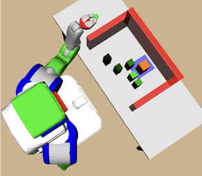
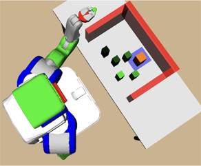
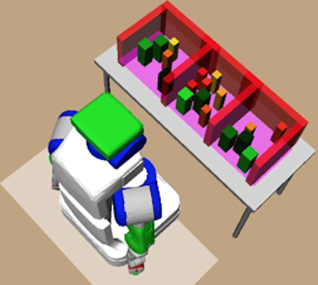
In a variety of important planning problems, however, these approaches fall short. Consider the problem in Figure 1(a), where the robot has to find a collision-free inverse kinematics solution to reach the orange object by reconfiguring the green objects. An unguided uniform sampling approach performs poorly since the state space is extremely high-dimensional, consisting of the combined configuration spaces of the robot and many objects. A gradient computation is also difficult, since the robot has to make choices that are both discrete, such as which object to move, and continuous, such as where to place the chosen object, making the problem’s optimization manifold non-smooth. This type of hybrid optimization problem is difficult to solve efficiently.

(a) An example of the reconfiguration task. The movable obstacles are colored green, and the target object is colored with orange.

(b) An example of the bin packing task. The color of objects indicate the order of placement, and the darker the earlier.

Figure 1: Examples of reconfiguration and bin packing. For both tasks, the robot can only grasp objects from the side.

A promising approach for such complex hybrid planning problems is to sample some predefined number of actions in each state, and then treat the resulting problem as a heuristic search over discrete states and actions. A reconsideration strategy, which reconsiders states that has been previously expanded, can be employed to guarantee completeness.

The main distinction from a search in discrete state and action spaces is that, in the discrete case, having a good heuristic function is sufficient for efficiently finding a solution. A perfect heuristic, for instance, would find a plan without any exploration. However, in the continuous state and action spaces this is not true; if there is a very small volume of actions that lead to the goal, then even with a perfect heuristic we might inefficiently sample actions and reject most of them. Moreover, if the heuristic is not perfect, as is typically the case, having samples in undesirable regions of the action space could lead to expanding nodes that do not efficiently lead to a goal state.

Based on this observation, our objective in this paper is to learn from search experience an action sampling distribution that will guide the search of a planner that has an imperfect heuristic. We use a generative adversarial network (GAN), a recent advance in generative model learning, to approximate this distribution (Goodfellow et al., 2014). Unlike other methods, a GAN only requires a forward pass through a neural network to generate a sample, and does not require any prior distributional assumptions. The main challenge in learning a generative model from search experience data is that in a successful episode of search, there is a large number of state and action pairs that we sample but are not known to be on a trajectory to the goal, and only a relatively small number of samples that are on a trajectory to the goal. We will refer to samples on a successful trajectory as on-target samples, to indicate that they are from a target distribution that we would like to learn, and the rest as off-target samples. While we could just use the small number of on-target samples, learning would be much more effective if we can find a way to use the abundant off-target samples as well.

In light of this, we propose a principled approach that can learn a generative model from both on- and off-target samples. To do this, we estimate the importance-ratio between the on-target and off-target distributions using both classes of samples. We then extend GAN to introduce a new generative-model learning algorithm, called generative adversarial network with direct importance estimation (GANDI), that uses the importance ratio to learn from not only on-target samples, but also from off-target samples. While this algorithm is domain independent, we will demonstrate its effectiveness in learning a target action-sampling distribution. We theoretically analyze how the importance-ratio estimation and the difference between target and non-target distributions affect the quality of the resulting approximate distribution.

We evaluate GANDI in three different planning problems that commonly occur in warehousing applications. We show that our algorithm outperforms a standard uniform sampler and a standard GAN in terms of planning and data efficiency.

Related work

Our work touches upon four different topics: continuous state-action space planning, learning to guide planning, importance-ratio estimation, and generative model learning. We provide descriptions of approaches in these areas that are closest to our problem in terms of motivation and technique.

In the area of continuous-space planning, there are several approaches that attempt to sample actions by employing optimistic optimization methods for black-box functions. Mansley et. al (2011) assign a hierarchical optimistic optimization (HOO) (Bubeck et al., 2009) agent at each state to decompose the action space to sample promising ones. A similar approach is taken by Buso̧niu et. al, (2013), where a simultaneous optimistic optimization (SOO) agent is assigned at each state (Munos., 2011). There are other approaches to more specialized continuous state and action problems, such as motion-planning and task-and-motion planning; these include sample-based methods (Kuffner and LaValle, 2000; Kavraki et al., 2000; Garrett, Kaelbling, and Lozano-Pérez, 2017; Vega-Brown and Roy, 2016), and gradient-based optimization methods  (Zucker et al., 2013; Schulman et al., 2014; Toussaint, 2015). The main objective of all these approaches is to construct, on-line, an optimal or a feasible plan without any off-line learning. No knowledge of solving one problem instance is transferred to another.

In learning to guide search, there is a large body of work that attempts to learn a policy or a value function off-line, and then use this information during an on-line search to make planning efficient. These methods are usually applied to discrete-action problems, where a recent prominent example is AlphaGo (Silver et al., 2016). In that paper, Silver et. al train a supervised policy off-line, using imitation learning and train a value function using self-play; they then guide Monte Carlo Tree Search (MCTS) in an on-line phase using these functions. In a similar line of work, Gelly et al. (2007) also integrates an off-line learned value function with MCTS. For learning to guide search in continuous-space planning problems, Kim et. al (2017) describe an approach for predicting constraints on the solution space rather than a value function or an action itself. The intuition is that a constraint is much more easily transferable across problem instances than a specific action in complex planning problems. We share this intuition, and we may view the learned action distribution as constraining the search space of a planning problem to promising regions.

Two recent advancements in generative-model learning, GANs (Goodfellow et al., 2014) and Variational Auto Encoders (VAEs) (Kingma and Welling, 2014), are appealing choices for learning an action-sampling distribution because inference is simply a feed-forward pass through a network. GANs are especially appealing, because for generic action spaces, we do not have any metric information available. VAEs, on the other hand, require a metric in an action space in order to compute the distance between a decoded sample and a true sample. Both of these methods require samples to be from a target distribution that one wishes to learn. Unfortunately, in our case we have limited access to samples from the target distribution, and this brings us to the importance-ratio estimation problem.

There is a long history of work that uses importance sampling to approximate desired statistics for a target distribution $p$ using samples from another distribution $q$, for example, in probabilistic graphical models (Koller and Friedman, 2009) and reinforcement learning problems (Precup, Sutton, and Dasgupta, 2001; Sutton and Barto, 1998). In these cases, we have a surrogate distribution $q$ that is cheaper to sample than the target distribution $p$. Our work shares the same motivation as these problems, in the sense that in search experience data, samples that are on successful trajectories are expensive to obtain, while other samples are relatively cheaper and more abundant.

Recently, importance-ratio estimation has been studied for the problem of covariate shift adaptation, which closely resembles our setting. Covariate shift refers to the situation where we have samples from a training distribution that is different from the target distribution. Usually, an importance-ratio estimation method (Kanamori, Hido, and Sugiyama, 2009; Sugiyama et al., 2008; Huang et al., 2007) is employed to re-weight the samples from the training distribution, so that it matches the target distribution for supervised learning. We list some prominent approaches here. In kernel-based methods for estimating the importance (Huang et al., 2007), authors try to match the mean of samples of $q$ and $p$ in a feature space, by re-weighting the samples from $q$. In the direct estimation approach, Sugiyama et al. (2008) try to minimize the KL divergence between the distributions $q$ and $p$ by re-weighting $q$. In another approach, Kanamori et al. (2009) directly minimize the least squares objective between the approximate importance-ratios and the target importance-ratios. All these formulations yield convex optimization problems, where the decision variables are parameters of a linear function that computes the importance weight for a given random variable. Our algorithm extends the direct estimation approach using a deep neural network, and then applies it for learning a generative model using off-and-on target samples.

Background

Planning in continuous spaces

A deterministic continuous action and state space planning problem is a tuple $[\mathcal{S},\mathcal{A},s_{0},G,T]$ where $\mathcal{S}$ and $\mathcal{A}$ are state and action spaces, $T:\mathcal{S}\times\mathcal{A}\rightarrow\mathcal{S}$ is a transition function that maps a state and an action to a next state, $s_{0}\in\mathcal{S}$ is the initial state and $G\subset\mathcal{S}$ is a goal set.

An instance of a planning problem consists of a tuple $(s_{0},G,\omega)$, where $\omega\in\Omega$ represents parameters of a problem instance. While the state changes according to $T$ when an action is executed, the parameters represent aspects of the problem that do not change within the given instance. For example, a state might represent poses of objects to be manipulated by a robot, while $\omega$ might represent their shapes. Given a planning problem instance, a heuristic state-space planner requires a heuristic function $H:\mathcal{S}\rightarrow\mathbb{R}$ that estimates a cost-to-go. This function might be learned, or designed by a user. The planning algorithm shown in Algorithm 1 describes an extension of discrete-space heuristic planner to continuous-spaces. This version of the algorithm is greedy with respect to $H$, but it is straightforward to arrange for a version that is more like A*, by taking path cost to the current state into account as well.

The key distinction from a discrete state-action space heuristic search algorithm is the action-sampling distribution $q_{a|s}$ and the reconsideration strategy for a node. While in the discrete case we push all the neighbors of the current node, here we sample $k$ actions and then push the resulting nodes. Without any domain-specific knowledge, $q_{a|s}$ is a uniform distribution in some bounded region in $\mathcal{A}(s,\omega)$ that depends on the current state and the parameters of the problem. The reconsideration strategy refers to pushing the node that we just popped back to the queue, in order to guarantee probabilistic completeness.

Given this setup, we can see that even a perfect heuristic will not be helpful unless good action samples are generated. Moreover, in most cases we have an imperfect heuristic function. This motivates the problem of learning an action-sampling distribution, which we formulate next by considering what information we can extract from search experience.

Algorithm 1 Search($s_{0},G,T,k,H,q_{a|s}$)

  $Q={\it InitQueue}({\it Node}(s_{0}))$

  while True do

     $n=Q.pop(\arg\min_{n\in Q}H(n.s))$ //dequeue the cheapest $n$

     if $n.s\in G$ then

        return $n$

     end if

     for $i\in 1..k$ do

        Sample $a\sim q_{a|s}(a\mid n.s)$

        $Q.push(Node(T(n.s,a))$

     end for

     $Q.push(n)$ // reconsideration

  end while

Problem formulation

Ideally, our objective would be to learn a distribution that assigns zero probability to actions that are not on an optimal trajectory to $G$, and non-zero probability to actions on an optimal trajectory. Such a distribution would yield a path to a goal without any exploration, regardless of the quality of the given heuristic function.

Unfortunately, in sufficiently difficult problems, optimal planners are not available, therefore it is impossible to determine whether an action was on an optimal path from the search-experience data. Thus, we consider an alternative objective: learn a distribution that assigns low probability to actions that lead to undesirable parts of the state space. We now examine two types of undesirable actions that lead to such states.

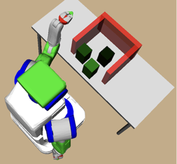
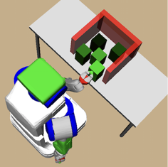
The first type is dead-end actions that lead to dead-end states. A state $s$ is a dead-end state if there is no feasible path from $s$ to a state in $G$. Dead-end states are clearly to be avoided if possible, because all search effort below them in the search tree is guaranteed to be wasted. An example of a dead-end state is shown in Figure 1(b). Here, the robot is asked to pack five objects into the relatively tight bin. It cannot move an object once it is placed, so if the robot places a first few objects in the front of the bin like in Figure 1(b) (left), then it will be in a dead-end state.

The second type is no-progress actions that transition to a state that has the same or greater true cost-to-go as the current state. An example is shown in Figure 1(a), where the robot has to reconfigure poses of the green objects to find a collision-free space to reach the orange object with its left arm. When the robot moves the light green object as shown in Figure 1(a) (left) to (right), this action does not constitute progress towards making room for reaching the target object.

Now, our objective is to learn an action distribution $p_{a|s}$ that assigns low probabilities to these two types of actions. We denote the $m$ search experience episodes for training data, collected using a domain-independent action sampler $q_{a|s}$, as $\Big{\{}\Big{[}(s_{i},a_{p}^{(i)})_{i=1}^{n_{p}},(s_{i},a_{q}^{(i)})_{i=1}^{n_{q}},(\omega^{(j)},s_{0}^{(j)},G^{(j)})\Big{]}\Big{\}}_{j=1}^{m}$ where $a_{p}^{(i)}$ is an action on the trajectory from $s_{0}^{(j)}$ to $s\in G^{(j)}$, $a_{q}^{(i)}$ is an action in the search tree, but not the solution trajectory, and $s_{i}$ is the state in which $a_{p}^{(i)}$ or $a_{q}^{(i)}$ was executed. $n_{p}$ and $n_{q}$ denote the number of state and action pairs that are on the trajectory to the goal and the rest, respectively.

Fortunately, the distribution of $(s,a)$ pairs on successful trajectories in the data has the following properties: they have zero probability assigned to dead-end states and actions, dead-end actions and states cannot occur on a path to the goal. They also have low probability assigned to no-progress actions, because most actions, though not necessarily all, are making progress. However, we cannot say anything about $(s,a)$ pairs not on a successful trajectory: they may or may not be desirable. Therefore, we will call the $a_{p}^{(i)}$ values on-target samples, and the $a_{q}^{(i)}$ as off-target samples. Our algorithm, GANDI, uses both of these two sources of data to learn a target distribution.

Generative Adversarial Networks

The objective of a GAN is to obtain a generator $G$ that transforms a random variable $z$, sampled usually from a Gaussian or a uniform distribution, to a random variable of interest which in our case is an action $a$. A GAN learns $p_{G}$, an approximation of the target distribution, which in our case is $p_{a|s}$. For the purpose of description of GAN, we will treat the distributions as unconditional; they can be directly extended to condition on $s$ by viewing the transformation as mapping $(s,z)$ to $a$.

We denote the on-target samples $\mathbf{A}_{p}:=\{a_{p}^{(i)}\}_{i=1}^{n_{p}}$, and the samples generated by $G$ as $\{a_{g}^{(i)}\}_{i=1}^{n_{g}}$. To learn the generator $G$, a GAN alternates between optimizing a function $D$, which tries to output 1 on on-target samples and output 0 on samples generated by $G$, and optimizing $G$, which tries to generate samples that cause $D$ to output 1. This leads to the following objectives:

$$D =\arg\min_{D}\sum_{i=1}^{n_{p}}\log D(a_{p}^{(i)})+\sum_{i=1}^{n_{g}}\log(1-D(a_{g}^{(i)}))$$ (1)

$$G =\arg\max_{G}\sum_{i=1}^{n_{g}}\log D(a_{g}^{(i)})$$ (2)

where $n_{p}=n_{g}$ to force $D$ to assume the classes are equally likely. After training, given a sample of $z\sim p_{z}$, the neural network $G(z)$ outputs $a$ with probability $p_{G}(a)$.

Direct importance ratio estimation

We now describe an approach to estimate importance weights between the target and uniform distribution, $w(a;s)=p_{a|s}(a|s)/q_{a|s}(a|s)$ using a deep neural network (DNN). If we had these weights, then we could use $\mathbf{A}_{q}$ to augment $\mathbf{A}_{p}$ used for training the generative model $p_{G}$ to approximate $p_{a|s}$. While there are several methods for estimating $w(a)$ (Huang et al., 2007; Kanamori, Hido, and Sugiyama, 2009; Sugiyama et al., 2008), we will use the least squares approach of Kanamori et al. (2009) because it integrates easily into DNN-based methods. In this approach, we approximate $w$ with $\hat{w}$ using the objective function

$$J(\hat{w}) =\int_{a}(\hat{w}(a)-w(a))^{2}q(a)da\,.$$

In practice, we optimize its sample approximation version, $\hat{J}(\hat{w})$, which yields

$$\hat{w} =\arg\min_{\hat{w}}\sum_{i=1}^{n_{q}}\hat{w}^{2}(a_{q}^{(i)})-2\sum_{i=1}^{n_{p}}\hat{w}(a_{p}^{(i)}),\text{ s.t }\hat{w}(a)\geq 0$$ (3)

where the constraint is enforced to keep the importance weights positive. Intuitively, $\hat{w}$ attempts to assign high values to $a_{p}^{(i)}$ and low values $a_{q}^{(i)}$, to the degree allowed by its hypothesis class.

The method was originally proposed to be used with a linear architecture, in which $\hat{w}(a)=\theta^{T}\phi(a)$; this implies there is a unique global optimum as a function of $\theta$, but requires a hand-designed feature representation $\phi(\cdot)$. For robot planning problems, however, manually designing features is difficult, while special types of DNN architectures, such as convolutional neural networks, may effectively learn a good representation. In light of this, we represent $\hat{w}$ with a DNN. The downside of this strategy is the loss of convexity with respect to the free parameters $\theta$, but we have found that the flexibility of representation offsets this problem.

Generative Adversarial Network with Direct Importance Estimation

In this section, we introduce our algorithm, GANDI, which can take advantage of off-target samples from $q_{a|s}$ using importance weights. We first describe how to formulate the objective for training GANs with importance weights. For the purpose of exposition, we begin by assuming we are given $w(a)$, and we only have samples from the off-target distribution, $\mathbf{A}_{q}$, and none from the target distribution. Using importance weights $w(a)$, the objective for the discriminator in GANs becomes

$$D =\arg\min_{D}\sum_{i=1}^{n_{q}}w(a_{q}^{(i)})\log D(a_{q}^{(i)})+\sum_{i=1}^{n_{g}}\log(1-D(a_{g}^{(i)}))$$ (4)

In trying to solve the equation 4, it is critical to have balanced training set sizes $n_{p}$ and $n_{g}$. In the importance weighted version of the GAN shown in equation 4, however, the sum of the weights $c=\sum_{i=1}^{n_{q}}w(a_{q}^{(i)})$, serves as an effective sample size for the data $\mathbf{A}_{q}$. To achieve a balanced objective, we might then select $n_{g}$ to be equal to c.

Taking this approach would require adjusting the the GAN objective function and modifying mini-batch gradient descent algorithm to use uneven mini-batch sizes in every batch in training, which is awkward in many high-performance NN software packages. Instead, we develop a method for bootstrapping $\mathbf{A}_{q}$ that allows us to use existing mini-batch gradient descent codes without modification. Specifically, instead of multiplying each off-target sample by its importance weight, we bootstrap (i.e. re-sample the data from $\mathbf{A}_{q}$ with replacement), with a probability $p_{w}(a)$, where $p_{w}(a)=\frac{w(a)}{\sum_{i=1}^{n_{q}}w(a_{q}^{(i)})}\,.$ This method allows us to generate a dataset $\hat{\mathbf{A}}$ in which the expected number of instances of each element of $\mathbf{A}$ is proportional to its importance weight. Moreover, since we bootstrap, the amount of training data remains the same, and $D$ now sees a balanced number of samples effectively drawn from $p(a)=w(a)q(a)$ and $p_{G}$.

One can show that $p_{w}$ is actually proportional to $p$.

Proposition 1

For $a\in\mathbf{A}_{q}$,

$$p_{w}(a)=k\cdot p(a)\text{ where }k=\frac{1}{\sum_{i=1}^{n_{q}}w(a_{q}^{(i)})}\,.$$

This means that samples drawn from the importance-reweighted data $\mathbf{A}$ can play the role of $\mathbf{A}_{p}$ in the GAN objective.

We now describe some practical details for approximating $w(a)$ with $\hat{w}(a)$, whose architecture is a DNN. Equation 3 can be readily solved by a mini-batch gradient-descent algorithm implemented using any readily available NN software package. The non-negativity constraint can also be straight-forwardly incorporated by simply using the rectified linear activation function at the output layer. Now, with estimated importance weights and bootstrapped samples, the objective for $D$ shown in equation 4 becomes

$$\hat{D}=\arg\min_{D}\sum_{i=1}^{n_{q}}D(a_{w}^{(i)})+\sum_{i=1}^{n_{g}}\log(1-D(a_{g}^{(i)}))\,,$$ (5)

where $a_{w}^{(i)}$ denotes a bootstrapped sample from $\mathbf{A}_{q}$, and $n_{q}=n_{g}$. This involves just using $\mathbf{A}_{q}$, but in practice, we also use $\mathbf{A}_{p}$, by simply augmenting the dataset $\mathbf{A}_{q}$ with $\mathbf{A}:=\mathbf{A}_{q}\cup\mathbf{A}_{p}$, and then applying $\hat{w}(\cdot)$ to $\mathbf{A}$ for bootstrapping, yielding final dataset $\hat{\mathbf{A}}$. Algorithm 2 contains the code for GANDI.

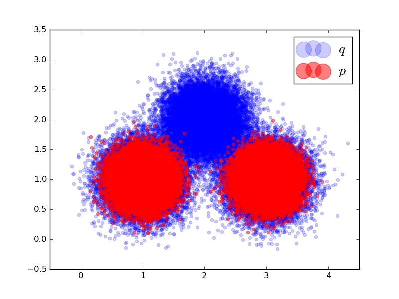
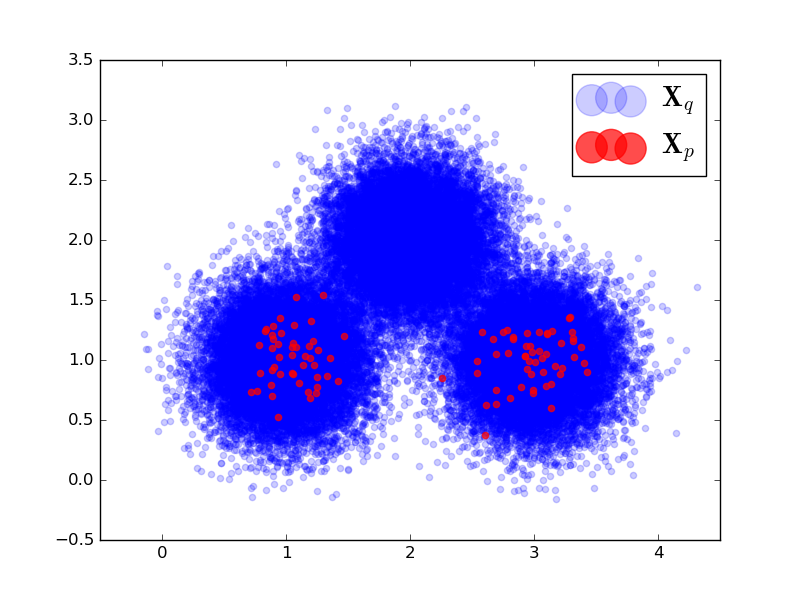
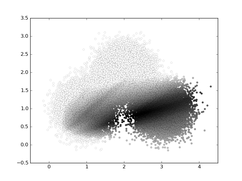
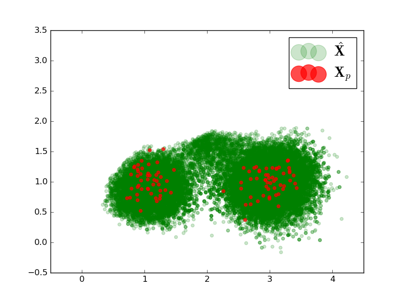
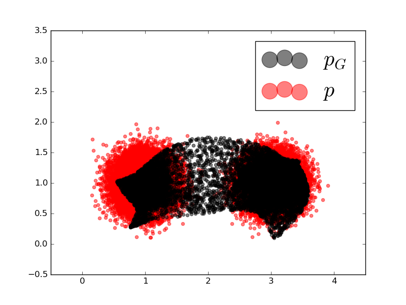
We illustrate the result of the bootstrapping with a simple example, shown in Figure 2, where we have a Gaussian mixture model for both on-and off-target distributions $p$ and $q$, where $p$ is a mixture of two Gaussians centered at $(1,1)$ and $(3,1)$, and $q$ is a mixture of three Gaussians at $(1,1),(3,1),$ and $(2,2)$ with larger variances than those of $p$.

(a) Distributions $p$ and $q$

(b) Off- and on-target samples

(c) Importance weights of $\mathbf{A}$.

(d) Bootstrapped samples

(e) $p_{G}$ and the target distribution $p$.

Figure 2: Example of importance weight estimation (c), bootstrapping (d), and samples from $p_{G}$ and $p$ (e) in an illustrative domain with Gaussian mixtures.

Algorithm 2 GANDI($\mathbf{A}_{p},\mathbf{A}_{q}$)

  $\hat{w}\leftarrow EstimateImportanceWeights(\mathbf{A}_{p},\mathbf{A}_{q})$ // objective (3) with on-and off-target samples $\mathbf{A}_{p}$ and $\mathbf{A}_{q}$

  $p_{w}(a):=\frac{\hat{w}(a)}{\sum_{i=1}^{n_{q}}\hat{w}(a_{q}^{(i)})+\sum_{i=1}^{n_{p}}\hat{w}(a_{p}^{(i)})}$ // define bootstrap probability distribution

  $\mathbf{A}\leftarrow\mathbf{A}_{p}\cup\mathbf{A}_{q}$

  $\hat{\mathbf{A}}\leftarrow Bootstrap(\mathbf{A},p_{w})$ // sample $\mathbf{A}$ with probability $p_{w}$, with replacement

  $G\leftarrow TrainGAN(\hat{\mathbf{A}})$ // train the GAN using objectives (1) and (2) with $\hat{\mathbf{A}}$ as on-target samples

  return $G$

Theoretical analysis

In this section, we analyze how error in importance estimation affects the performance of $p_{G}$ in approximating $p$. The basic result on GANs, shown in the limit of infinite data, representational and computational capacity, is that $p_{G}$ converges to $p$ (Goodfellow et al., 2014), although subsequent papers have presented more subtle form of analysis (Arjovsky and Bottou, 2017).

Now, under the same assumptions, we consider the effect of using importance weighted off-target data. If $w$ is exact, then $p(a)=w(a)q(a)$ and the GAN objective is unchanged. If, however, we use an estimation of importance weighting function $\hat{w}$, then the objective of $\hat{D}$, the importance-weight corrected discriminator, differs from $D$ and they achieve different solutions.

We wish to analyze the effect of importance estimation error on KL and reverse-KL divergence between $p$ and $p_{G}$. First, define $\rho=\sup_{a\in\mathcal{A}_{p}}q(a)/p(a)$, where $\mathcal{A}_{p}$ is the support of $p$. We can see that $\rho>=1$, with equality occurring when $p(a)=q(a)$ for all $a$.

For the KL divergence, we have the following theorem.

Theorem 1

If $w(a)\geq\epsilon\ \forall a\in\mathcal{A}_{q}$, and $J(\hat{w})\leq\epsilon^{2}$, then

$${\rm KL}(p||p_{G})\leq\log\Big{(}\frac{1}{1-\epsilon\rho}\Big{)}\;\;.$$

Note that $0\leq\epsilon\rho\leq 1$ due to the condition $w(a)\geq\epsilon$. For reverse KL we have:

Theorem 2

If $J(\hat{w})\leq\epsilon^{2}$, $KL(p_{G}||p)\leq(1+\epsilon)\log(1+\epsilon\rho)$ .

The proofs are included in the supplementary material.

These theorems imply three things: (1) If $w=\hat{w}$, then $\epsilon=0$, and both divergences go to 0, regardless of $\rho$; (2) If $p=q$, then the error in importance weight estimation is the only source of error in modeling $p$ with $p_{G}$. This error can be arbitrarily large, as $\epsilon$ becomes large; and (3) If $p\neq q$ then $\rho>1$, and it contributes to the error in modeling $p$ with $p_{G}$.

Experiments

We validate GANDI on three different robot planning tasks that involve continuous state and action spaces and finite depths. The purpose of these experiments is to verify the hypothesis that learning an action sampling distribution improves planning efficiency relative to a standard uniform sampler, and a GANDI is more data efficient than a standard GAN that is only trained with on-target samples.

We have three tasks that might occur in a warehouse. The first is a bin-packing task, where a robot has to pack different numbers of objects of different sizes into a relatively tight bin. The second task is to stow objects into crowded bins, where there already are obstacles. The final task is a reconfiguration task, where a robot needs to reconfigure five randomly placed moveable objects in order to make room to reach a target object. In the first two tasks, the robot is not allowed to move the objects once they are placed, which leads to a large volume of dead-end states that cause wasted computational effort for a planner with an uniform action sampler. In the third task, we have no dead-end states, but a planner could potentially waste computational effort in trying no-progress actions. For all tasks, the robot is only allowed to grasp objects from the side; this is to simulate a common scenario in a warehouse environment, with objects in a place covered on top, such as a shelf. For the first two experiments, we use depth-first-search. This is equivalent to having a heuristic that estimates a cost-to-go by number of objects placed, since we cannot move objects once they are placed. For the last experiment we use breadth-first-search as our planner, since there is no simple heuristic function evident. For all cases, the number of action samples per node, $k$, is 3. We use Algorithm 1 with a given action sampler.

Throughout the three tasks, we compare three different action samplers in terms of success rate within a given time limit: the uniform sampler that uniformly samples an action from a specified action space, a standard GAN trained only with on-target samples, and GANDI, which is trained with both on and off-target samples. We use the same architecture for both the standard GAN and GANDI, and perform 100 repetitions to obtain the 95% confidence intervals for all the plots. The architecture description is in the appendix.

A crucial drawback of generative adversarial networks is that they lack an evaluation metric; thus it is difficult to know when to stop training. We deal with this by testing weights from all epochs on 10 trials, and then picking the weights with the best performance, with which we performed 100 additional repetitions to compute the success rates.

(a) GAN’s action sampling distribution

(b) GANDI’s action sampling distribution

(c) A GANDI’s action distribution

(d) A stow domain problem instance

Figure 3: The left two figures show examples from the bin packing domain when 20 episodes of training data are used. Green indicates the on-target samples, and blue indicates the learned distributions. Figure 3(c) shows an action distribution for the reconfiguration domain when given 35 training episodes.

(a) The bin packing domain

(b) The stow domain

(c) The reconfiguration domain

Figure 4: Plots of success rate vs. number of training episodes for all three tasks

Bin packing problem

In this task, a robot has to move 5, 6, 7 or 8 objects into a region of size 0.3m by 1m (width by length). The size of each object is uniformly random between 0.05m to 0.11m, depending on how many objects the robot has to pack. A problem instance is defined by the number of objects and the size of each object, $\omega=[n_{obj},O_{size}]$. A state is defined by the object placements. For a given problem instance, all objects have the same size. An example of a solved problem instance with $n_{obj}=5$ and $O_{size}=0.11$m is given in Figure 1(b) (right).

The action space consists of the two dimensional (x,y) locations of objects inside the bin, and a uniform action sampler uniformly samples these values from this region. The robot base is fixed. The planning depth varies from 5 to 8, depending on how many objects need to be placed. This means that plans consist of 10 to 16 decision variables. Clearly, there is a large of volume of dead-end actions: any action that puts objects down in the front of the bin early will lead to a dead-end state.

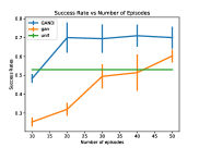
Figure 4(a) shows the comparison among GANDI, standard GAN, and uniform action sampling in terms of success rate when given 5.0 seconds to solve a problem instance. We can see the data efficiency of GANDI: with 20 training episodes, it outperforms the uniform sampler, while a standard GAN requires 50 training episodes to do so. The uniform sampler can only solve about 50% of the problem instances within this time limit, while GANDI can solve more than 70%.

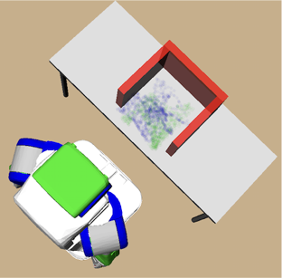
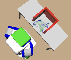
We also compare the distributions for GAN and GANDI when the same number of training data are given. Figures 3(a) and 3(b) show 1000 samples from GAN and GANDI for packing 5 objects. While GANDI learns to avoid the front-middle locations, GAN is still close to a uniform distribution, and has a lot of samples in this region which lead to dead-end states. GANDI focuses its samples to the corners at the back or the front so that it has spaces for all 5 objects.

Stowing objects into crowded bins

In this task, a robot has to stow 8 objects into three different bins, where there already are 10 obstacles. A bin is of size 0.4m by 0.3m, an obstacle is of size 0.05m by 0.05m, and the objects to be placed down are all of size 0.07m by 0.07m. A problem instance is defined by the (x,y) locations of 10 obstacles, each of which is randomly distributed in one of the bins. Figure 3(d) shows an instance of a solved stow problem.

The action space for this problem consists of (x,y) locations of an object to be placed, and the robot’s (x,y) base pose. This makes 4 dimensional continuous action-space. The planning depth is always 8, for placing 8 objects. Thus plans consist of of 36 continuous decision variables. Again, there is a large volume of dead-end actions, similarly to the previous problem: putting objects down without consideration of poses of later objects can potentially block collision-free paths for placing them.

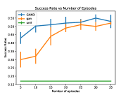
Figure 4(b) compares the success rates of the algorithms with a 30-seconds time limit for planning. For the uniform sampler, we sample first an object placement pose, and then sample a base pose that can reach the object at its new location without colliding with other objects. Unlike the previous task, learning-based approaches significantly outperform the uniform sampling approach for this task. This is because there is an unstated constraint between the object placement location and base pose, which is that the location must be within a reachable distance from the sampled robot base pose. Again, we can observe the data efficiency of GANDI compared to GAN. When the number of training data points is small, it outperforms it.

Reconfiguration planning in a tight space

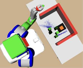
In this task, a robot has to reconfigure movable obstacles out of the way in order to find a collision-free inverse-kinematics solution for its left-arm to reach the target object. There are five movable obstacles in this problem, each with size 0.05m by 0.05m, and the target object of size 0.07m by 0.07m, and the reconfiguration must happen within a bin, which is of size 0.7m by 0.4m. A problem instance is defined by (x,y) locations of the movable obstacles and the target object. The movable obstacles are randomly distributed within the bin; the target object location is distributed along the back of the bin. Figure 3(c) shows an example of a rearrangement problem instance at its initial state, with the black region indicating the distribution of target object locations.

An action specification consists of one discrete value and two continuous values: what object to move and the (x,y) placement pose of the object being moved. There is no fixed depth. For both the uniform random sampler and the learned generative model, we uniformly at random choose an object to move. The robot base is fixed, and the robot is not allowed to use its right arm.

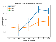
Figure 4(c) compares the success rates of the algorithms with a 10-seconds time limit for planning. In this problem, the learning based approaches outperform the uniform sampler even with a small number of training data points. The relationship between GANDI and GAN is similar to the previous experiment, except that GANDI and GAN are within the each other’s confidence interval when a small number of training points are used. Eventually, GANDI comes to clearly outperform GAN.

We would like to know if GANDI’s distribution indeed assigns low probabilities to no-progress actions. In Figure 3(c), we show GANDI’s distribution of obsject placements after training on 35 episodes. The left top corner of the bin is empty because there are no collision-free inverse-kinematics solution for that region . As the figure shows, there are no placement samples in front of the target object, but only on the sides that would contribute to clearing space for the robot’s left arm to reach the target object.

Conclusion

We presented GANDI, a generative model learning algorithm that uses both on-target and cheaper off-target samples for data efficiency using importance-ratio estimation. We provided guarantees on how the error in importance-ratio estimation affects the performance of the learned model, and illustrated that this learning algorithm is effective for learning an action sampling distribution for guiding the search of a planner in difficult robot planning problems.

References

- Arjovsky and Bottou (2017) Arjovsky, M., and Bottou, L. 2017. Towards principled methods for training generative adversarial networks. In International Conference on Learning Representations.
- Bubeck et al. (2009) Bubeck, S.; Munos, R.; Stoltz, G.; and Szepesvári, C. 2009. Online optimization in X-armed bandits. In Advances in Neural Information Processing Systems.
- Buso̧niu et al. (2013) Buso̧niu, L.; Daniels, A.; Munos, R.; and Babuška, R. 2013. Optimistic planning for continuous-action deterministic systems. In Adaptive Dynamic Programming And Reinforcement Learning.
- Garrett, Kaelbling, and Lozano-Pérez (2017) Garrett, C. R.; Kaelbling, L. P.; and Lozano-Pérez, T. 2017. Sample-based methods for factored task and motion planning. In Robotics: Science and Systems.
- Gelly and Silver (2007) Gelly, S., and Silver, D. 2007. Combining online and offline knowledge in UCT. International Conference on Machine learning.
- Goodfellow et al. (2014) Goodfellow, I.; Pouget-Abadie, J.; Mirza, M.; Xu, B.; Warde-Farley, D.; Ozair, S.; Courville, A.; and Bengio, Y. 2014. Generative adversarial nets. In Advances in Neural Information Processing Systems.
- Huang et al. (2007) Huang, J.; Smola, A.; Gretton, A.; Borgwardt, K.; and Schölkopf, B. 2007. Correcting sample selection bias by unlabeled data. In Advances in Neural Information Processing Systems.
- Kanamori, Hido, and Sugiyama (2009) Kanamori, T.; Hido, S.; and Sugiyama, M. 2009. A least-squares approach to direct importance estimation. Journal of Machine Learning Research 10.
- Kavraki et al. (2000) Kavraki, L. E.; Svestka, P.; Latombe, J.; and Overmars, M. H. 2000. Probabilistic roadmaps for path planning in high-dimensional configuration spaces. IEEE Transactions on Robotics and Automation 12.
- Kim, Kaelbling, and Lozano-Pérez (2017) Kim, B.; Kaelbling, L. P.; and Lozano-Pérez, T. 2017. Learning to guide task and motion planning using score-space representation. In International Conference on Robotics and Automation.
- Kingma and Welling (2014) Kingma, D. P., and Welling, M. 2014. Auto-encoding variational bayes. In International Conference on Learning Representations.
- Koller and Friedman (2009) Koller, D., and Friedman, N. 2009. Probabilistic Graphical Models: Principles and Techniques. The MIT Press.
- Kuffner and LaValle (2000) Kuffner, J., and LaValle, S. 2000. RRT-connect: An efficient approach to single-query path planning. In International Conference on Robotics and Automation.
- Mansley, Weinstein, and Littman (2011) Mansley, C.; Weinstein, A.; and Littman, M. L. 2011. Sample-based planning for continuous action Markov decision processes. In International Conference on Planning and Scheduling.
- Munos. (2011) Munos., R. 2011. Optimization of deterministic functions without the knowledge of its smoothness. In Advances in Neural Information Processing Systems.
- Precup, Sutton, and Dasgupta (2001) Precup, D.; Sutton, R.; and Dasgupta, S. 2001. Off-policy temporal-difference learning with function approximation. In International Conference on Machine Learning.
- Schulman et al. (2014) Schulman, J.; Duan, Y.; Ho, J.; Lee, A.; Awwal, I.; Bradlow, H.; Pan, J.; Patil, S.; Goldberg, K.; and Abbeel, P. 2014. Motion planning with sequential convex optimization and convex collision checking. International Journal on Robotics Research.
- Silver et al. (2016) Silver, D.; Huang, A.; Maddison, C.; Guez, A.; Sifre, L.; van den Driessche, G.; Schrittwieser, J.; Antonoglou, I.; Panneershelvam, V.; Lanctot, M.; Dieleman, S.; Grewe, D.; Nham, J.; Kalchbrenner, N.; Sutskever, I.; Lillicrap, T.; Leach, M.; Kavukcuoglu, K.; Graepel, T.; and Hassabis, D. 2016. Mastering the game of Go with deep neural networks and tree search. Nature.
- Sugiyama et al. (2008) Sugiyama, M.; Nakajima, S.; H. Kashima, P. B.; and Kawananbe, M. 2008. Direct importance estimation with model selection and its application to covariate shift adaptation. In Advances in Neural Information Processing Systems.
- Sutton and Barto (1998) Sutton, R., and Barto, A. G. 1998. Reinforcement Learning: An Introduction. A Bradford Book.
- Toussaint (2015) Toussaint, M. 2015. Logic-geometric programming: An optimization-based approach to combined task and motion planning. In International Joint Conference on Artificial Intelligence.
- Vega-Brown and Roy (2016) Vega-Brown, W., and Roy, N. 2016. Asymptotically optimal planning under piecewise-analytic constraints. In Workshop on the Algorithmic Foundations of Robotics.
- Zucker et al. (2013) Zucker, M.; Ratliff, N.; Dragan, A.; Pivtoraiko, M.; Klingensmith, M.; Dellin, C.; Bagnell, J. A.; and Srinivasa, S. 2013. CHOMP: Covariant hamiltonian optimization for motion planning. International Journal on Robotics Research.