Likelihood Analysis of the Sub-GUT MSSM in Light of LHC 13-TeV Data

Abstract

We describe a likelihood analysis using MasterCode of variants of the MSSM in which the soft supersymmetry-breaking parameters are assumed to have universal values at some scale $M_{\rm in}$ below the supersymmetric grand unification scale $M_{\rm GUT}$, as can occur in mirage mediation and other models. In addition to $M_{\rm in}$, such ‘sub-GUT’ models have the 4 parameters of the CMSSM, namely a common gaugino mass $m_{1/2}$, a common soft supersymmetry-breaking scalar mass $m_{0}$, a common trilinear mixing parameter $A$ and the ratio of MSSM Higgs vevs $\tan\beta$, assuming that the Higgs mixing parameter $\mu>0$. We take into account constraints on strongly- and electroweakly-interacting sparticles from $\sim 36$/fb of LHC data at 13 TeV and the LUX and 2017 PICO, XENON1T and PandaX-II searches for dark matter scattering, in addition to the previous LHC and dark matter constraints as well as full sets of flavour and electroweak constraints. We find a preference for $M_{\rm in}\sim 10^{5}$ to $10^{9}\,\,\mathrm{GeV}$, with $M_{\rm in}\sim M_{\rm GUT}$ disfavoured by $\Delta\chi^{2}\sim 3$ due to the ${\rm BR}(B_{s,d}\to\mu^{+}\mu^{-})$ constraint. The lower limits on strongly-interacting sparticles are largely determined by LHC searches, and similar to those in the CMSSM. We find a preference for the LSP to be a Bino or Higgsino with $m_{\tilde{\chi}^{0}_{1}}\sim 1\,\,\mathrm{TeV}$, with annihilation via heavy Higgs bosons $H/A$ and stop coannihilation, or chargino coannihilation, bringing the cold dark matter density into the cosmological range. We find that spin-independent dark matter scattering is likely to be within reach of the planned LUX-Zeplin and XENONnT experiments. We probe the impact of the $(g-2)_{\mu}$ constraint, finding similar results whether or not it is included.

KCL-PH-TH/2017-45, CERN-PH-TH/2017-197, DESY 17-156, IFT-UAM/CSIC-17-089
FTPI-MINN-17/19, UMN-TH-3703/17

1 Introduction

Models invoking the appearance of supersymmetry (SUSY) at the TeV scale are being sorely tested by the negative results of high-sensitivity searches for sparticles at the LHC [1, 2] and for the scattering of dark matter particles [3, 4, 5, 6]. There have been many global analyses of the implications of these experiments for specific SUSY models, mainly within the minimal supersymmetric extension of the Standard Model (MSSM), in which the lightest supersymmetric particle (LSP) is stable and a candidate for dark matter (DM). This may well be the lightest neutralino, $\tilde{\chi}^{0}_{1}$ [7], as we assume here. Some of these studies have assumed universality of the soft SUSY-breaking parameters at the GUT scale, e.g., in the constrained MSSM (the CMSSM) [8, 9, 10, 11] and in models with non-universal Higgs masses (the NUHM1,2) [9, 12]. Other analyses have taken a phenomenological approach, allowing free variation in the soft SUSY-breaking parameters at the electroweak scale (the pMSSM) [13, 14, 15, 16].

A key issue in the understanding of the implications of the LHC searches for SUSY is the exploration of regions of parameter space where compressed spectra may reduce the sensitivity of searches for missing transverse energy, $/E_{T}$. These regions also have relevance to cosmology, since models with sparticles that are nearly degenerate with the LSP allow for important coannihilation processes that suppress the relic LSP number density, allowing heavier values of $m_{\tilde{\chi}^{0}_{1}}$. The accompanying heavier SUSY spectra are also more challenging for the LHC $/E_{T}$ searches.

The CMSSM offers limited prospects for coannihilation, and examples that have been studied in some detail include coannihilation with the lighter stau slepton, $\tilde{\tau}_{1}$ [17, 18], or the lighter stop squark, $\tilde{t}_{1}$ [19]. Other models offer the possibilities of different coannihilation partners, such as the lighter chargino, $\tilde{\chi}^{\pm}_{1}$ [20, 14], some other slepton [16] or squark flavour [21], or the gluino [22, 23]. In particular, the pMSSM allows for all these possibilities, potentially also in combination [16].

In this paper we study the implications of LHC and DM searches for an intermediate class of SUSY models, in which universality of the soft SUSY-breaking parameters is imposed at some input scale $M_{\rm in}$ below the GUT scale $M_{\rm GUT}$ but above the electroweak scale [24, 25], which we term ‘sub-GUT’ models. Models in this class are well motivated theoretically, since the soft SUSY-breaking parameters in the visible sector may be induced by some dynamical mechanism such as gluino condensation that kicks in below the GUT scale. Specific examples of sub-GUT models include warped extra dimensions [26] and mirage mediation [27].

Mirage mediation can occur when two sources of supersymmetry breaking play off each other, such as moduli mediation based, e.g., on moduli stabilization as in [28] and anomaly mediation [29]. The relative contributions of each source of supersymmetry breaking can be parametrized by the strength of the moduli mediation, $\alpha$, and allows one to interpolate between nearly pure moduli mediation (large $\alpha$) and nearly pure anomaly mediation ($\alpha\to 0$). For example, gaugino masses, $M_{i}$, can be written as $M_{i}=M_{s}(\alpha+b_{i}g_{i}^{2})$ where $M_{s}$ is related to the gravitino mass in anomaly mediation ($m_{3/2}=16\pi^{2}M_{s}$), and $b_{i},g_{i}$ are the beta functions and gauge couplings. This leads to a renormalization scale, $M_{in}=M_{GUT}e^{-8\pi^{2}/\alpha}$ at which gaugino masses and soft scalar masses take unified values, although there is no physical threshold at $M_{in}$ in this model. We are not concerned here with the detailed origin of $M_{in}$, simply postulating that there is a scale below the GUT scale where the supersymmetry breaking masses are unified.

Sub-GUT models are of particular phenomenological interest, since the reduction in the amount of renormalization-group (RG) running below $M_{\rm in}$, compared to that below $M_{\rm GUT}$ in the CMSSM and related models, leads naturally to SUSY spectra that are more compressed [24]. These may offer extended possibilities for ‘hiding’ SUSY via suppressed $/E_{T}$ signatures, as well as offering enhanced possibilities for different coannihilation processes. Other possible effects of the reduced RG running include a stronger lower limit on $m_{\tilde{\chi}^{0}_{1}}$ because of the smaller hierarchy with the gluino mass, a stronger lower limit on the DM scattering cross section because of a smaller hierarchy between $m_{\tilde{\chi}^{0}_{1}}$ and the squark masses, and greater tension between LHC searches and a possible SUSY explanation of the measurement of $(g-2)_{\mu}$ [30, 31], because of the smaller hierarchies between the gluino and squark masses and the smuon and $\tilde{\chi}^{0}_{1}$ masses.

We use the MasterCode framework [8, 9, 12, 14, 32, 21, 33, 16, 34, 35] to study these issues in the sub-GUT generalization of the CMSSM, which has 5 free parameters, comprising $M_{\rm in}$ as well as a common gaugino mass $m_{1/2}$, a common soft SUSY-breaking scalar mass $m_{0}$, a common trilinear mixing parameter $A$ and the ratio of MSSM Higgs vevs $\tan\beta$, assuming that the Higgs mixing parameter $\mu>0$, as may be suggested by $(g-2)_{\mu}$ . Our global analysis takes into account the relevant CMS searches for strongly-and electroweakly-interacting sparticles with the full 2016 sample of $\sim 36$/fb of data at 13 TeV [36, 37, 38], and also considers the available results of searches for long-lived charged particles [39, 40] . We also include a complete set of direct DM searches published in 2017, including the PICO limit on the spin-dependent scattering cross section, $\sigma^{\rm SD}_{p}$ [4], as well as the first XENON1T limit [5] and the most recent PandaX-II limit [6] on the spin-independent scattering cross section, $\sigma^{\rm SI}_{p}$, as well as the previous LUX search [3]. We also include full sets of relevant electroweak and flavour constraints.

We find in our global sub-GUT analysis a distinct preference for $M_{W}\ll M_{\rm in}\ll M_{\rm GUT}$, with values of $M_{\rm in}\sim 10^{5}$ or $\sim 10^{8}$ to $10^{9}\,\,\mathrm{GeV}$ being preferred by $\Delta\chi^{2}\sim 3$ compared to the CMSSM (where $M_{\rm in}=M_{\rm GUT}$). This preference is driven principally by the ability of the sub-GUT MSSM to accommodate a value of ${\rm BR}(B_{s,d}\to\mu^{+}\mu^{-})$ smaller than in the Standard Model (SM), as preferred by the current data [41, 42, 43]. As discussed later, this effect can be traced to the different RGE evolution of $A_{t}$ in the sub-GUT model, which enables it have a different sign from that in the CMSSM. The lower limits on strongly-interacting sparticles are similar to those in the CMSSM, being largely determined by LHC searches. The favoured DM scenario is that the LSP is a Bino or Higgsino with $m_{\tilde{\chi}^{0}_{1}}\sim 1\,\,\mathrm{TeV}$, with the cold DM being brought into the cosmological range by annihilation via heavy Higgs bosons $H/A$ and stop coannihilation, or chargino coannihilation. In contrast to the CMSSM and pMSSM11, the possibility that $m_{\tilde{\chi}^{0}_{1}}\ll 1\,\,\mathrm{TeV}$ is strongly disfavoured in the sub-GUT model, so the LHC constraints have insignificant impact. The same is true of the LHC searches for long-lived charged particles.

The likelihood functions for fits with and without the $(g-2)_{\mu}$ constraint are quite similar, reflecting the anticipated difficulty in accounting for the $(g-2)_{\mu}$ anomaly in the sub-GUT MSSM. Encouragingly, we find a preference for a range of $\sigma^{\rm SI}_{p}$ just below the current upper limits, and within the prospective sensitivities of the LUX-Zeplin (LZ) [44] and XENONnT [45] experiments.

The outline of this paper is as follows. In Section 2 we summarize the experimental and astrophysical constraints we apply. Since we follow exactly our treatments in [16], we refer the interested reader there for details. Then, in Section 3 we summarize the MasterCode framework and how we apply it to the sub-GUT models. Our results are presented in Section 4. Finally, Section 5 summarizes our conclusions and discusses future perspectives for the sub-GUT MSSM.

2 Experimental and Astrophysical Constraints

2.1 Electroweak and Flavour Constraints

Our treatments of these constraints are identical to those in [16], which were based on Table 1 of [21] with the updates listed in Table 2 of [16]. Since we pay particular attention in this paper to the impact on the sub-GUT parameter space of the $(g-2)_{\mu}$ constraint [30], we note that we assume

$$a_{\mu}^{\rm EXP}-a_{\mu}^{\rm SM}\;=\;(30.2\pm 8.8\pm 2.0_{\rm{MSSM}})\times 10^{-10}$$ (1)

to be the possible discrepancy with SM calculations [31] that may be explained by SUSY. As we shall see, the ${\rm BR}(B_{s,d}\to\mu^{+}\mu^{-})$ measurement [41, 42, 43] plays an important role in indicating a preferred region of the sub-GUT parameter space.

2.2 Higgs Constraints

In the absence of published results on the Higgs boson based on Run 2 data, we use in this global fit the published results from Run 1 [46], as incorporated in the HiggsSignals code [47].

Searches for heavy MSSM Higgs bosons are incorporated using the HiggsBounds code [48], which uses the results from Run 1 of the LHC. We also include the ATLAS limit from $\sim 36$/fb of data from the LHC at 13 TeV [49].

2.3 Dark Matter Constraints and
Mechanisms

Cosmological density

Since $R$-parity is conserved in the MSSM, the LSP is a candidate to provide the cold DM (CDM). We assume that the LSP is the lightest neutralino $\tilde{\chi}^{0}_{1}$ [7], and that it dominates the total CDM density. For the latter we assume the Planck 2015 value: $\Omega_{\rm CDM}h^{2}=0.1186\pm 0.0020_{\rm EXP}\pm 0.0024_{\rm TH}$ [50].

Density mechanisms

As in [16], we use the following set of measures related to particle masses to indicate when specific mechanisms are important for bringing $\Omega_{\rm CDM}h^{2}$ into the Planck 2015 range, which have been validated by checks using Micromegas [51].

$\bullet$Chargino coannihilation

This may be important if the $\tilde{\chi}^{0}_{1}$ is not much lighter than the lighter chargino, $\tilde{\chi}^{\pm}_{1}$, and we introduce the following coannihilation measure:

$${\rm chargino}{\rm~{}coann.~{}:}\qquad\left(\frac{m_{\tilde{\chi}^{\pm}_{1}}}{m_{\tilde{\chi}^{0}_{1}}}-1\right)\,<\,0.25\,.$$ (2)

We shade green in the 2-dimensional plots in Section 4 the parts of the 68 and 95% CL regions where (2) is satisfied.

$\bullet$Rapid annihilation via direct-channel $H/A$ poles

We find that LSP annihilation is enhanced significantly if the following condition is satisfied:

$$H/A{\rm~{}funnel~{}:}\qquad\left|\frac{M_{A}}{m_{\tilde{\chi}^{0}_{1}}}-2\right|\,<\,0.1\,,$$ (3)

and shade in blue the parts of the 68 and 95% CL regions of the two-dimensional plots in Section 4 where (3) is satisfied.

$\bullet$Stau coannihilation

We introduce the following measure for stau coannihilation:

$${{\tilde{\tau}}}{\rm~{}coann.~{}:}\qquad\left(\frac{m_{\tilde{\tau}_{1}}}{m_{\tilde{\chi}^{0}_{1}}}-1\right)\,<\,0.15\,,$$ (4)

and shade in pink the corresponding area of the 68 and 95% CL regions of the two-dimensional sub-GUT parameter planes. We do not find regions where coannihilation with other charged slepton species, or with sneutrinos, is important.

$\bullet$Stop coannihilation

We introduce the following measure for stop coannihilation:

$${{\tilde{t}_{1}}}{\rm~{}coann.~{}:}\qquad\left(\frac{m_{\tilde{t}_{1}}}{m_{\tilde{\chi}^{0}_{1}}}-1\right)\,<\,0.15\,,$$ (5)

and shade in yellow the corresponding area of the 68 and 95% CL regions of the two-dimensional sub-GUT parameter planes. We do not find regions where coannihilation with other squark species, or with gluinos, is important.

$\bullet$Focus-point region

The sub-GUT parameter space has a focus-point region where the DM annihilation rate is enhanced because the LSP $\tilde{\chi}^{0}_{1}$ has an enhanced Higgsino component as a result of near-degeneracy in the neutralino mass matrix. We introduce the following measure to characterize this possibility:

$${\rm focus~{}point~{}:}\qquad\left(\frac{\mu}{m_{\tilde{\chi}^{0}_{1}}}\right)-1\,<\,0.3\,,$$ (6)

and shade in cyan the corresponding area of the 68 and 95% CL regions of the two-dimensional sub-GUT parameter planes.

$\bullet$Hybrid regions

In addition to regions where one of the above DM mechanisms is dominant, there are also various ‘hybrid’ regions where more than one mechanism is important. These are indicated in the two-dimensional planes below by shadings in mixtures of the ‘primary’ colours above, which are shown in the corresponding figure legends. For example, there are prominent regions where both chargino coannihilation and direct-channel $H/A$ poles are important, whose shading is darker than the blue of regions where $H/A$ poles are dominant.

Direct DM searches

We apply the constraints from direct searches for weakly-interacting dark matter particles via both spin-independent and -dependent scattering on nuclei. In addition to the 2016 LUX constraint on $\sigma^{\rm SI}_{p}$ [3], we use the 2017 XENON1T [5] and PandaX-II [6] constraints on the spin-independent DM scattering, which we combine in a joint two-dimensional likelihood function in the $(m_{\tilde{\chi}^{0}_{1}},\sigma^{\rm SI}_{p})$ plane. We estimate the spin-independent nuclear scattering matrix element assuming $\sigma_{0}=36\pm 7\,\,\mathrm{MeV}$ and $\Sigma_{\pi N}=50\pm 7\,\,\mathrm{MeV}$ as in [52, 53] , and the spin-dependent nuclear scattering matrix element assuming $\Delta u=+0.84\pm 0.03,\Delta d=-0.43\pm 0.03$ and $\Delta s=-0.09\pm 0.03$ [52, 53]. We implement the recent PICO [4] constraint on the spin-dependent dark matter scattering cross-section on protons, $\sigma^{\rm SD}_{p}$.

Indirect astrophysical searches for DM
As discussed in [16], there are considerable uncertainties in the use of IceCube data [56] to constrain $\sigma^{\rm SD}_{p}$ and, as we discuss below, the global fit yields a prediction that lies well below the current PICO [4] constraint on $\sigma^{\rm SD}_{p}$ and the current IceCube sensitivity, so we do not include the IceCube data in our global fit.

2.4 13 TeV LHC Constraints

Searches for gluinos and squarks

We implement the CMS simplified model searches with $\sim 36$/fb of data at 13 TeV for events with jets and $/E_{T}$ but no leptons [36] and for events with jets, $/E_{T}$ and a single lepton [37], using the Fastlim approach [57]. We use [36] to constrain ${\tilde{g}}{\tilde{g}}\to[q{\bar{q}}\tilde{\chi}^{0}_{1}]^{2}$ and $[b{\bar{b}}\tilde{\chi}^{0}_{1}]^{2}$, and ${\tilde{q}}{\tilde{\bar{q}}}\to[q\tilde{\chi}^{0}_{1}][{\bar{q}}\tilde{\chi}^{0}_{1}]$, and use [37] to constrain ${\tilde{g}}{\tilde{g}}\rightarrow[t{\bar{t}}\tilde{\chi}^{0}_{1}]^{2}$. Details are given in [16].

Stop and sbottom searches

We also implement the CMS simplified model searches with $\sim 36$/fb of data at 13 TeV in the jets + 0 [36] and 1 [37] lepton final states to constrain ${\tilde{t}_{1}}{\tilde{\bar{t}}}_{1}\to[t\tilde{\chi}^{0}_{1}][{\bar{t}}\tilde{\chi}^{0}_{1}]$, $[c\tilde{\chi}^{0}_{1}][{\bar{c}}\tilde{\chi}^{0}_{1}]$ in the compressed-spectrum region, $[bW^{+}\tilde{\chi}^{0}_{1}][{\bar{b}}W^{-}\tilde{\chi}^{0}_{1}]$ via $\tilde{\chi}^{\pm}_{1}$ intermediate states and ${\tilde{b}_{1}}{\tilde{\bar{b}}}_{1}\to[b\tilde{\chi}^{0}_{1}][{\bar{b}}\tilde{\chi}^{0}_{1}]$, again using Fastlim as described in detail in [16].

Searches for electroweak inos

We also consider the CMS searches for electroweak inos in multilepton final states with $\sim 36$/fb of data at 13 TeV [38], constraining $\tilde{\chi}^{\pm}_{1}\tilde{\chi}^{0}_{2}\to[W\tilde{\chi}^{0}_{1}][Z\tilde{\chi}^{0}_{1}],3\ell^{\pm}+2\tilde{\chi}^{0}_{1}$ via ${\tilde{\ell}}^{\pm}/\tilde{\nu}$ intermediate states, and $3\tau^{\pm}+2\tilde{\chi}^{0}_{1}$ via ${\tilde{\tau}}^{\pm}$ intermediate states using Fastlim [57] as described in [16]. These analyses can also be used to constrain the production of electroweak inos in the decays of coloured sparticles, since these searches do not impose conditions on the number of jets. However, as we discuss below, in the sub-GUT model the above-mentioned searches for strongly-interacting sparticles impose such strong limits on the $m_{\tilde{\chi}^{0}_{1}}$ and $m_{\tilde{\chi}^{\pm}_{1}}$ that the searches for electroweak inos do not have significant impact on the preferred parameter regions.

Searches for long-lived or stable charged particles

We also consider a posteriori the search for long-lived charged particles published in [39], which are sensitive to lifetimes $\gtrsim$ ns, and the search for massive charged particles that escape from the detector without decaying [40]. However, these also do not have significant impact on the preferred parameter regions, as we discuss in detail below, and are not included in our global fit.

3 Analysis Framework

3.1 Model Parameters

As mentioned above, the five-dimensional sub-GUT MSSM parameter space we consider in this paper comprises a gaugino mass parameter $m_{1/2}$, a soft SUSY-breaking scalar mass parameter $m_{0}$ and a trilinear soft SUSY-breaking parameter $A_{0}$ that are assumed to be universal at some input mass scale $M_{\rm in}$, and the ratio of MSSM Higgs vevs, $\tan\beta$. Table 1 displays the ranges of these parameters sampled in our analysis, as well as their divisions into segments, which define boxes in the five-dimensional parameter space.

Parameter	Range	# of
		segments
$M_{\rm in}$	$(10^{3},10^{16})\,\,\mathrm{GeV}$	6
$m_{1/2}$	$(0,6)\,\,\mathrm{TeV}$	2
$m_{0}$	$(0,6)\,\,\mathrm{TeV}$	2
$A_{0}$	$(-15,10)\,\,\mathrm{TeV}$	2
$\tan\beta$	( 1 , 60)	2
Total # of boxes		96

Table 1: The ranges of the sub-GUT MSSM parameters sampled, together with the numbers of segments into which they are divided, together with the total number of sample boxes shown in the last row. This sample is for positive values of the Higgs mixing parameter, $\mu$. As already noted, a smaller sample for $\mu<0$ gives similar results. Note that our sign convention for $A$ is opposite to that used in SoftSusy [58].

3.2 Sampling Procedure

We sample the boxes in the five-dimensional sub-GUT MSSM parameter space using the MultiNest package [59], choosing for each box a prior such that 80% of the sample has a flat distribution within the nominal box, and 20% of the sample is in normally-distributed tails extending outside the box. This eliminates features associated with the boundaries of the 96 boxes, by providing a smooth overlap between them. In total, our sample includes $\sim 112$ million points with $\Delta\chi^{2}<100$.

3.3 The MasterCode

The MasterCode framework [8, 9, 12, 14, 32, 21, 33, 16, 34, 35], interfaces and combines consistently various private and public codes using the SUSY Les Houches Accord (SLHA) [60]. This analysis uses the following codes: SoftSusy 3.7.2 [58] for the MSSM spectrum, FeynWZ [61] for the electroweak precision observables, SuFla [62] and SuperIso [63] for flavour observables, FeynHiggs 2.12.1-beta [64] for $(g-2)_{\mu}$ and calculating Higgs properties, HiggsSignals 1.4.0 [47] and HiggsBounds 4.3.1 [48] for experimental constraints on the Higgs sector, Micromegas 3.2 [51] for the DM relic density, SSARD [53] for the spin-independent and -dependent elastic scattering cross-sections $\sigma^{\rm SI}_{p}$ and $\sigma^{\rm SD}_{p}$, SDECAY 1.3b [65] for sparticle branching ratios and (as already mentioned) Fastlim [57] to recast LHC 13 TeV constraints on events with $/E_{T}$.

4 Results

4.1 Results for $\mathbf{M_{\rm in},m_{0}}$ and $\mathbf{m_{1/2}}$

Figure 1: Profile likelihood functions in the sub-GUT MSSM. Top left: One-dimensional profile likelihood function for $M_{\rm in}$. Top right: Two-dimensional projection of the likelihood function in the $(m_{0},m_{1/2})$ plane. Middle left: Two-dimensional projection of the likelihood function in the $(M_{\rm in},m_{0})$ plane. Middle right: Two-dimensional projection of the likelihood function in the $(M_{\rm in},m_{1/2})$ plane. Bottom left: One-dimensional profile likelihood function for $m_{0}$. Bottom right: One-dimensional profile likelihood function for $m_{1/2}$. Here and in subsequent one-dimensional plots, the solid lines include the constraints from $\sim 36$/fb of LHC data at 13 TeV and the dashed lines drop them, and the blue lines include $(g-2)_{\mu}$, whereas the green lines drop these constraints. Here and in subsequent two-dimensional plots, the red (blue) (green) contours are boundaries of the 1-, 2- and 3-$\sigma$ regions, and the shadings correspond to the DM mechanisms indicated in the legend.

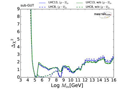
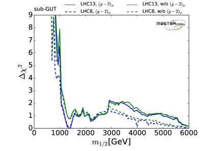
The top left panel of Fig. 1 displays the one-dimensional profile $\chi^{2}$ likelihood function for $M_{\rm in}$, as obtained under various assumptions . In this and subsequent one-dimensional plots, the solid lines represent the results of a fit including results from $\sim 36$/fb of data from the LHC at 13 TeV (LHC13), whereas the dashed lines omit these results, and the blue lines include $(g-2)_{\mu}$, whereas the green lines are obtained when this constraint is dropped.

We observe in the top left panel of Fig. 1 a preference for $M_{\rm in}\simeq 4.2\times 10^{8}\,\,\mathrm{GeV}$ when the LHC 13-TeV data and $(g-2)_{\mu}$ are both included (solid blue line), falling to $\simeq 5.9\times 10^{5}\,\,\mathrm{GeV}$ when the 13-TeV data are dropped (dashed blue line). There is little difference between the global $\chi^{2}$ values at these two minima, but values of $M_{\rm in}<10^{5}\,\,\mathrm{GeV}$ are strongly disfavoured. The rise in $\Delta\chi^{2}$ when $M_{\rm in}$ increases to $\sim 10^{6}\,\,\mathrm{GeV}$ and the LHC 13-TeV data are included (solid lines) is largely due to the contribution of ${\rm BR}(B_{s,d}\to\mu^{+}\mu^{-})$. At lower $M_{\rm in}$, the $H\to\tau^{+}\tau^{-}$ constraint allows a larger value of $\tan\beta$, which leads (together with an increase in the magnitude of $A$) to greater negative interference in the supersymmetric contribution to ${\rm BR}(B_{s,d}\to\mu^{+}\mu^{-})$, as preferred by the data.

For both fits including the LHC 13-TeV data (solid lines), the $\Delta\chi^{2}$ function $\sim 1$ for most of the range $M_{\rm in}\in(10^{5},10^{11})\,\,\mathrm{GeV}$, apart from localized dips, whereas $\Delta\chi^{2}$ rises to $\gtrsim 2$ for $M_{\rm in}\gtrsim 10^{12}\,\,\mathrm{GeV}$. As already mentioned and discussed in more detail later, the reduction in the global $\chi^{2}$ function for $M_{\rm in}\lesssim 10^{12}\,\,\mathrm{GeV}$ arises because for these values of $M_{\rm in}$ the sub-GUT model can accommodate better the measurement of ${\rm BR}(B_{s,d}\to\mu^{+}\mu^{-})$, whose central experimental value is somewhat lower than in the SM.

When the $(g-2)_{\mu}$ constraint is dropped, as shown by the green lines in top left panel of Fig. 1, there is a minimum of $\chi^{2}$ around $M_{\rm in}\simeq 1.6\times 10^{5}\,\,\mathrm{GeV}$, whether the LHC 13-TeV constraint is included, or not. The values of the other input parameters at the best-fit points with and without these data are also very similar, as are the values of $\Delta\chi^{2}$. On the other hand, the values of $\Delta\chi^{2}$ for $M_{\rm in}\in(10^{5},10^{8})\,\,\mathrm{GeV}$ are generally smaller when the LHC 13-TeV constraints are dropped, the principal effect being due to the $H/A\to\tau^{+}\tau^{-}$ constraint.

In contrast, when $M_{\rm in}\gtrsim 10^{9}\,\,\mathrm{GeV}$ the $\Delta\chi^{2}$ function in the top left panel of Fig. 1 is quite similar whether the LHC 13-TeV and $(g-2)_{\mu}$ constraints are included or not, though $\Delta\chi^{2}\gtrsim 0.5$ lower when the $(g-2)_{\mu}$ constraint is dropped, as seen by comparing the green and blue lines. This is because the tension between $(g-2)_{\mu}$ and LHC data is increased when $M_{3}/M_{1}$ is reduced, as occurs because of the smaller RGE running when $M_{\rm in}<M_{\rm GUT}$. Conversely, lower $M_{\rm in}$ is relatively more favoured when $(g-2)_{\mu}$ is dropped, leading to this increase in $\Delta\chi^{2}$ at high $M_{\rm in}$ though the total $\chi^{2}$ is reduced.

We list in Table 2 the parameters of the best-fit points when we drop one or both of the $(g-2)_{\mu}$ and LHC13 constraints, as well as the values of the global $\chi^{2}$ function at the best-fit points. We see that the best-fit points without $(g-2)_{\mu}$ are very similar with and without the LHC 13-TeV constraint. On the other hand, the best-fit points with $(g-2)_{\mu}$ have quite different values of the other input parameters, as well as larger values of $M_{\rm in}$, particularly when the LHC 13-TeV data are included.

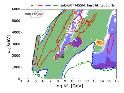
The top right panel of Fig. 1 displays the $(m_{0},m_{1/2})$ plane when the $(g-2)_{\mu}$ and LHC13 constraints are applied. Here and in subsequent planes, the green star indicates the best-fit point, whose input parameters are listed in Table 2: it lies in a hybrid stop coannihilation and rapid $H/A$ annihilation region.

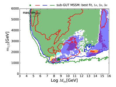
This parameter plane and others in Fig. 1 and subsequent figures also display the 68% CL (1-$\sigma$), 95% CL (2-$\sigma$) and 99.7% (3-$\sigma$) contours in the fit including both $(g-2)_{\mu}$ and the LHC13 data as red, blue and green lines, respectively. We note, here and subsequently, that the green 3-$\sigma$ contours are generally close to the blue 2-$\sigma$ contours, indicating a relatively rapid increase in $\chi^{2}$, and that the $\chi^{2}$ function is relatively flat for $m_{0},m_{1/2}\gtrsim 1\,\,\mathrm{TeV}$. The regions inside the 95% CL contours are colour-coded according to the dominant DM mechanisms, as shown in the legend beneath Fig. 1 . Similar results for this and other planes are obtained when either or both of the $(g-2)_{\mu}$ and LHC13 constraints are dropped.

We see that chargino coannihilation is important in the upper part of the $(m_{0},m_{1/2})$ plane shown in the top right panel of Fig. 1, but rapid annihilation via the $H/A$ bosons becomes important for lower $m_{1/2}$, often hybridized with other mechanisms including stop and stau coannihilation. We also note smaller regions with $m_{1/2}\sim 1.5$ to $3\,\,\mathrm{TeV}$ where stop coannihilation and focus-point mechanisms are dominant.

	$m_{0}$ [GeV]	$m_{1/2}$ [GeV]	$A_{0}$ [GeV]	$\tan\beta$	$M_{in}$ [GeV]	$\chi^{2}$
With $(g-2)_{\mu}$
With 13-TeV	1940	1370	- 6860	36	$4.1\times 10^{8}$	99.56
Without 13-TeV	1620	6100	- 8670	45	$5.7\times 10^{5}$	99.38
Without $(g-2)_{\mu}$
With 13-TeV	3550	6560	- 14400	45	$1.6\times 10^{5}$	88.73
Without 13-TeV	3340	6390	- 14260	45	$1.6\times 10^{5}$	88.67

Table 2: Values of the sub-GUT input parameters at the best-fit points with and without $(g-2)_{\mu}$ and the LHC 13-TeV data.

The middle left panel of Fig. 1 shows the corresponding $(M_{\rm in},m_{0})$ plane, where we see a significant positive correlation between the variables that is particularly noticeable in the 68% CL region. In most of this and the 95% CL region with $M_{\rm in}\lesssim 10^{13}\,\,\mathrm{GeV}$ the relic LSP density is controlled by chargino coannihilation, though with patches where rapid annihilation via the $A/H$ bosons is important, partly in hybrid combinations. In contrast, the $(M_{\rm in},m_{1/2})$ plane shown in the middle right panel of Fig. 1 does not exhibit a strong correlation between the variables. We see again the importance of chargino coannihilation, with the $A/H$ mechanism becoming more important for lower $m_{1/2}$ and larger $M_{\rm in}$, and for all values of $m_{1/2}$ for $M_{\rm in}\gtrsim 10^{14}\,\,\mathrm{GeV}$.

Also visible in the middle row of planes are small regions with $M_{\rm in}\sim 10^{13}$ to $10^{14}\,\,\mathrm{GeV}$ where stau coannihilation is dominant, partly hybridized with stop coannihilation. The reduction in the global $\chi^{2}$ function for $M_{\rm in}\lesssim 10^{12}\,\,\mathrm{GeV}$ visible in the top left panel of Fig. 1 is associated with the 68% CL regions in this range of $M_{\rm in}$ visible in the two middle planes of Fig. 1.

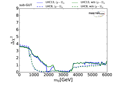
The one-dimensional profile likelihood functions for $m_{0}$ and $m_{1/2}$ are shown in the bottom panels of Fig. 1. We note once again the similarities between the results with/without $(g-2)_{\mu}$ (blue/green lines) and the LHC13 constraints (solid/dashed lines). The flattening of the $\chi^{2}$ function for $m_{0}$ at small values reflects the extension to $m_{0}=0$ of the 95% CL region in the top right panel of Fig. 1. On the other hand, the $\chi^{2}$ function for $m_{1/2}$ rises rapidly at small values, reflecting the close spacing of the 95 and 99.7% CL contours for $m_{1/2}\sim 1\,\,\mathrm{TeV}$ seen in the same plane. The impact of the LHC13 constraints is visible in the differences between the solid and dashed curves at small $m_{0}$, in particular. The $(g-2)_{\mu}$ constraint has less impact, as shown by the smaller differences between the green and blue curves. We see that the $\chi^{2}$ function for $m_{0}$ rises by $\gtrsim 1$ at large mass values, whereas that for $m_{1/2}$ falls monotonically at large values. The $\chi^{2}$ function for $m_{1/2}$ exhibits a local maximum at $m_{1/2}\sim 3\,\,\mathrm{TeV}$, which corresponds to the separation between the two 68% CL regions in the top right plane of Fig. 1. These are dominated by chargino coannihilation (larger $m_{1/2}$, green shading) and by rapid annihilation via $A/H$ bosons (smaller $m_{1/2}$, blue shading) and other mechanisms, respectively.

4.2 Squarks and gluinos

Figure 2: One-dimensional profile likelihood functions for $m_{\tilde{g}}$ (upper left panel), $m_{\tilde{q}_{R}}$ (upper right panel), $m_{\tilde{t}_{1}}$ (lower left panel) and $m_{\tilde{b}_{1}}$ (lower right panel).

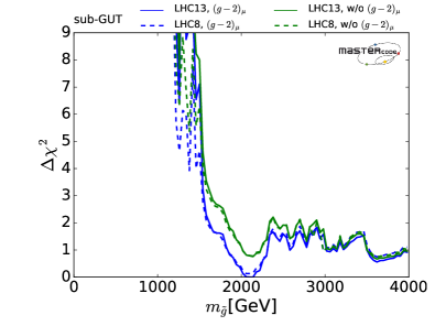
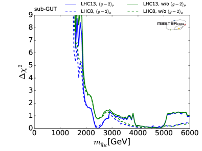
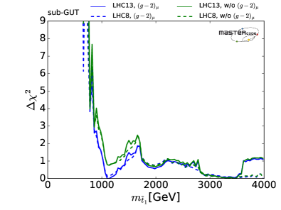
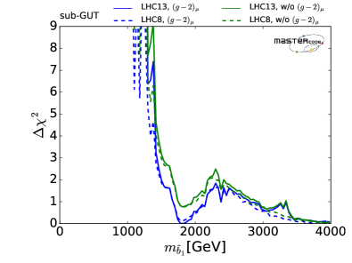
The various panels of Fig. 2 show the limited impact of the LHC 13-TeV constraints on the possible masses of strongly-interacting sparticles in the sub-GUT model, comparing the solid and dashed curves. The upper left panel shows that the 95% CL lower limit on $m_{\tilde{g}}\sim 1.5\,\,\mathrm{TeV}$, whether the LHC 13-TeV data and the $(g-2)_{\mu}$ constraint are included or not. However, the best-fit value of $m_{\tilde{g}}$ increases from $\sim 2\,\,\mathrm{TeV}$ to a very large value when $(g-2)_{\mu}$ is dropped, although the $\Delta\chi^{2}$ price for $m_{\tilde{g}}\sim 2\,\,\mathrm{TeV}$ is $\sim 1$. The upper right panel shows similar features in the profile likelihood function for $m_{\tilde{q}_{R}}$ (that for $m_{\tilde{q}_{L}}$ is similar), with a 95% CL lower limit of $\sim 2\,\,\mathrm{TeV}$, which is again quite independent of the inclusion of $(g-2)_{\mu}$ and the 13-TeV data. The lower panels of Fig. 2 show the corresponding profile likelihood functions for $m_{\tilde{t}_{1}}$ (left panel) and $m_{\tilde{b}_{1}}$ (right panel). We see that these could both be considerably lighter than the gluino and the first- and second-generation squarks, with 95% CL lower limits $m_{\tilde{t}_{1}}\sim 900\,\,\mathrm{GeV}$ and $m_{\tilde{b}_{1}}\sim 1.5\,\,\mathrm{TeV}$, respectively.

4.3 The lightest neutralino and lighter chargino

Figure 3: One-dimensional profile likelihood functions for $m_{\tilde{\chi}^{0}_{1}}$ (top left panel) and $m_{\tilde{\chi}^{\pm}_{1}}$ (top right panel), $m_{\tilde{\chi}^{\pm}_{1}}-m_{\tilde{\chi}^{0}_{1}}$ (middle left panel) the $\tilde{\chi}^{\pm}_{1}$ lifetime (middle right panel) and $M_{A}$ (bottom left panel). The bottom right panel shows the regions of the $(m_{\tilde{\chi}^{\pm}_{1}},\tau_{\tilde{\chi}^{\pm}_{1}})$ plane with $\tau_{\tilde{\chi}^{\pm}_{1}}\geq 10^{-15}$ s that are allowed in the fit including the $(g-2)_{\mu}$ and LHC 13-TeV constraints at the 68 (95) (99.7)% CL in 2 dimensions, i.e., $\Delta\chi^{2}<2.30(5.99)(11.83)$, enclosed by the red (blue) (green) contour.

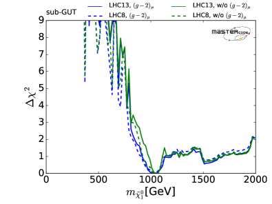
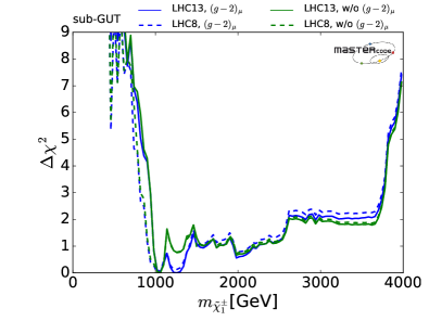
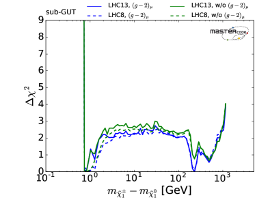
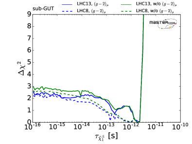
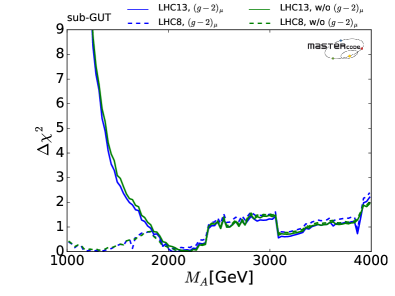
The top left panel of Fig. 3 shows the profile likelihood function for $m_{\tilde{\chi}^{0}_{1}}$, and the top right panel shows that for $m_{\tilde{\chi}^{\pm}_{1}}$. We see that in all the cases considered (with and without the $(g-2)_{\mu}$ and LHC13 constraints), the value of $\Delta\chi^{2}$ calculated using the LHC constraints on strongly-interacting sparticles is larger than $4$ for $m_{\tilde{\chi}^{0}_{1}}\lesssim 750\,\,\mathrm{GeV}$ and $m_{\tilde{\chi}^{\pm}_{1}}\lesssim 800\,\,\mathrm{GeV}$. Therefore, the LHC electroweakino searches [38] have no impact on the 95% CL regions in our 2-dimensional projections of the sub-GUT parameter space, and we do not include the results of [38] in our global fit.

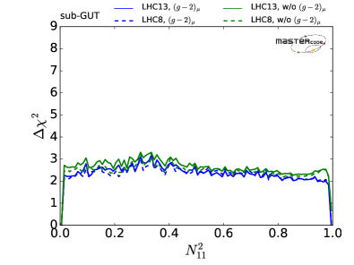
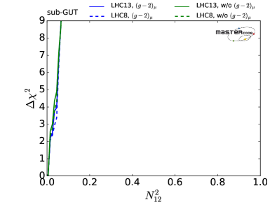
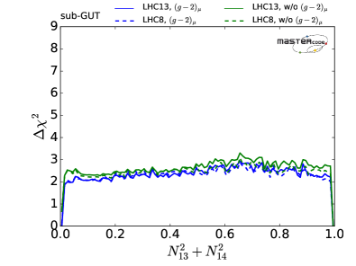
We now examine the profile likelihood functions for the fractions of Bino, Wino and Higgsino in the $\tilde{\chi}^{0}_{1}$ composition:

$$\tilde{\chi}^{0}_{1}\;=\;N_{11}{\tilde{B}}+N_{12}{\tilde{W}^{3}}+N_{13}{\tilde{H}_{u}}+N_{14}{\tilde{H}_{d}}\,,$$ (7)

which are shown in Fig. 4. As usual, results from an analysis including the 13-TeV data are shown as solid lines and without them as dashed lines, with $(g-2)_{\mu}$ as blue lines and without it as green lines. The top left panel shows that in the LHC 13-TeV case with $(g-2)_{\mu}$ an almost pure $\tilde{B}$ composition of the $\tilde{\chi}^{0}_{1}$ is preferred, $N_{11}\to 1$, though the possibility that this component is almost absent is only very slightly disfavoured. Conversely, before the LHC 13-TeV data there was a very mild preference for $N_{11}\to 0$, and this is still the case if $(g-2)_{\mu}$ is dropped. The upper right panel shows that a small $\tilde{W}^{3}$ component in the $\tilde{\chi}^{0}_{1}$ is strongly preferred in all cases. Finally, the lower panel confirms that small $\tilde{H}_{u,d}$ components are preferred when the LHC 13-TeV and $(g-2)_{\mu}$ constraints are applied, but large $\tilde{H}_{u,d}$ components are preferred otherwise.

Figure 4: Plots of the one-dimensional profile likelihood for the $\tilde{B}$ fraction in the LSP $\tilde{\chi}^{0}_{1}$ (upper left), for the $\tilde{W}^{3}$ fraction (upper right) and for the $\tilde{H}_{u,d}$ fraction (lower panel).

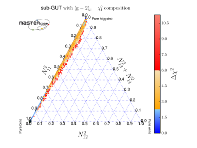
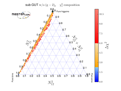
The $\tilde{\chi}^{0}_{1}$ compositions favoured at the 1-, 2- and 3-$\sigma$ levels (blue, yellow and red) are displayed in Fig. 5 for fits including LHC 13-TeV data with (without) the $(g-2)_{\mu}$ constraint in the left (right) panel. We see that these regions are quite similar in the two panels, and correspond to small Wino admixtures. On the other hand, the Bino fraction $N_{11}^{2}$ and the Higgsino fraction $N_{13}^{2}+N_{14}^{2}$ are relatively unconstrained at the 95% CL. The best-fit points are indicated by green stars, and the left panel shows again that in the fit with $(g-2)_{\mu}$ the LSP is an almost pure Bino, whereas an almost pure Higsino composition is favoured in the fit without $(g-2)_{\mu}$, as also seen in Table 3. These two extremes have very similar $\chi^{2}$ values in each of the fits displayed.

Figure 5: Triangular presentations of the $\tilde{\chi}^{0}_{1}$ composition in the fit with LHC 13-TeV including (dropping) the $(g-2)_{\mu}$ constraint in the left (right) panel. The 1-, 2- and 3-$\sigma$ regions in the plots are coloured blue, yellow and red, and the best-fit points are indicated by green stars.

	$\tilde{B}$	$\tilde{W}_{3}$	$\tilde{H}_{u}$	$\tilde{H}_{d}$
With $(g-2)_{\mu}$
With 13-TeV	0.999	-0.010	0.041	-0.025
Without 13-TeV	0.007	-0.011	0.707	-0.707
Without $(g-2)_{\mu}$
With 13-TeV	0.006	-0.010	0.707	-0.707
Without 13-TeV	0.007	-0.011	0.707	-0.707

Table 3: Composition of the $\tilde{\chi}^{0}_{1}$ LSP at the best-fit points with and without $(g-2)_{\mu}$ and the LHC 13-TeV data.

The global $\chi^{2}$ function is minimized for $m_{\tilde{\chi}^{0}_{1}}\simeq 1.0\,\,\mathrm{TeV}$, which is typical of scenarios with a Higgsino-like LSP whose density is brought into the Planck 2015 range by coannihilation with a nearly-degenerate Higgsino-like chargino $\tilde{\chi}^{\pm}_{1}$. Indeed, we see in the top right panel of Fig. 3 that $\chi^{2}$ is minimized when also $m_{\tilde{\chi}^{\pm}_{1}}\simeq m_{\tilde{\chi}^{0}_{1}}\simeq 1.0\,\,\mathrm{TeV}$. Table  3 displays the LSP composition of the sub-GUT model at the best-fit points with and without $(g-2)_{\mu}$and the LHC 13-TeV data. We see again that the $\tilde{\chi}^{0}_{1}$ LSP is mainly a Higgsino with almost equal $\tilde{H}_{u}$ and $\tilde{H}_{d}$ components, except in the fit with both LHC 13-TeV data and $(g-2)_{\mu}$ included, in which case it is an almost pure Bino.

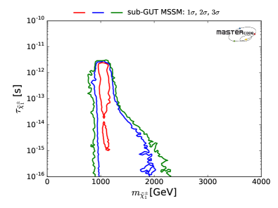
Looking at the middle left panel of Fig. 3, we see that the best-fit point has a chargino-LSP mass difference that may be ${\cal O}(1)\,\,\mathrm{GeV}$ or $\sim 200$ to $300\,\,\mathrm{GeV}$, with similar $\chi^{2}$ in all the cases considered, namely with and without the $(g-2)_{\mu}$ and LHC13 constraints. As seen in the middle right panel of Fig. 3, in the more degenerate case the preferred chargino lifetime $\tau_{\tilde{\chi}^{\pm}_{1}}\sim 10^{-12}$ s. The current LHC searches for long-lived charged particles [39] therefore do not impact this chargino coannihilation region, and are also not included in our global fit.

The top right panel of Fig. 3 displays an almost-degenerate local minimum of $\chi^{2}$ with $m_{\tilde{\chi}^{\pm}_{1}}\sim 1.3\,\,\mathrm{TeV}$, corresponding to a second, local minimum of $\chi^{2}$ where $m_{\tilde{\chi}^{\pm}_{1}}-m_{\tilde{\chi}^{0}_{1}}\sim 200$ to $300\,\,\mathrm{GeV}$, as seen in the middle left panel. In this region the relic density is brought into the Planck 2015 range by rapid annihilation through $A/H$ bosons, as can be inferred from the bottom left panel of Fig. 3, where we see that at this secondary minimum $M_{A}\simeq 2\,\,\mathrm{TeV}\simeq 2m_{\tilde{\chi}^{0}_{1}}$. The $\tilde{\chi}^{\pm}_{1}$ lifetime in this region is too short to appear in the middle and bottom right panels of Fig. 3, and too short to have a separated vertex signature at the LHC.

Finally, the bottom right panel of Fig. 3 shows the regions of the $(m_{\tilde{\chi}^{\pm}_{1}},\tau_{\tilde{\chi}^{\pm}_{1}})$ plane with $\tau_{\tilde{\chi}^{\pm}_{1}}\in(10^{-16},10^{-10})$ s that are allowed in the fit including the $(g-2)_{\mu}$ and LHC 13-TeV constraints at the 68 (95) (99.7) % CL in 2 dimensions, i.e., $\Delta\chi^{2}<2.30(5.99)(11.83)$. Since the chargino would decay into a very soft track and a neutralino, detecting a separated vertex in the region around the best-fit point would be very challenging.

4.4 Sleptons

Figure 6: One-dimensional profile likelihood functions for $m_{\tilde{\mu}_{R}}$ (upper left panel), $m_{\tilde{\tau}_{1}}$ (upper right panel) and $m_{\tilde{\tau}_{1}}-m_{\tilde{\chi}^{0}_{1}}$ (lower left panel). The lower right panel shows the $(m_{\tilde{\tau}_{1}},\tau_{\tilde{\tau}_{1}})$ plane, colour-coded as indicated in the right-hand legend. The 68 (95) (99.7)% CL regions in 2 dimensions, i.e., $\Delta\chi^{2}<2.30(5.99)(11.83)$, are enclosed by the red (blue) (green) contours.

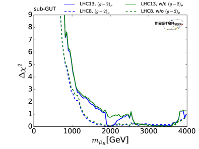
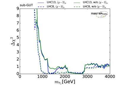
The upper left panel of Fig. 6 shows the profile likelihood function for $m_{\tilde{\mu}_{R}}$ (that for $m_{\tilde{e}_{R}}$ is indistinguishable, the ${\tilde{\mu}_{L}}$ and ${\tilde{e}_{L}}$ are slightly heavier). We see that in the sub-GUT model small values of $m_{\tilde{\mu}_{R}}$ were already disfavoured by earlier LHC data (dashed lines), and that this tendency has been reinforced by the LHC 13-TeV data (compare the solid lines). The same is true whether the $(g-2)_{\mu}$ constraint is included or dropped (compare the blue and green curves).

The upper right panel Fig. 6 shows the corresponding profile likelihood function for $m_{\tilde{\tau}_{1}}$, which shares many similar features. However, we note that the $\chi^{2}$ function for $m_{\tilde{\tau}_{1}}$ is generally lower than that for $m_{\tilde{\mu}_{R}}\in(1,2)\,\,\mathrm{TeV}$, though the 95% lower limits on $m_{\tilde{\tau}_{1}}$ and $m_{\tilde{\mu}_{R}}$ are quite similar, and both are $\simeq 1\,\,\mathrm{TeV}$ when the LHC 13-TeV constraints are included in the fit.

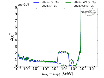
The lower left panel of Fig. 6 shows that very small values of $m_{\tilde{\tau}_{1}}-m_{\tilde{\chi}^{0}_{1}}$ in the stau coannihilation region are allowed at the $\Delta\chi^{2}\sim 1$ level in all the fits with the $(g-2)_{\mu}$ constraint, rising to $\Delta\chi^{2}\gtrsim 2$ for $m_{\tilde{\tau}_{1}}-m_{\tilde{\chi}^{0}_{1}}\gtrsim 20\,\,\mathrm{GeV}$ when the LHC 13-TeV data are included.

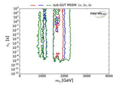
The lower right panel of Fig. 6 shows the $(m_{\tilde{\tau}_{1}},\tau_{\tilde{\tau}_{1}})$ plane, where we see that $\tau_{\tilde{\tau}_{1}}\in(10^{-7},10^{3})$ s is allowed at the 68% CL, for $1600\,\,\mathrm{GeV}\lesssim m_{\tilde{\tau}_{1}}\lesssim 2000\,\,\mathrm{GeV}$ and at the 95% CL also for $m_{\tilde{\tau}_{1}}\sim 1100\,\,\mathrm{GeV}$. This region of parameter space is close to the tip of the stau coannihilation strip. Lower ${\tilde{\tau}_{1}}$ masses are strongly disfavoured by the LHC constraints, particularly at 13 TeV, as seen in the upper right panel of Fig. 6. The heavier ${\tilde{\tau}_{1}}$ masses with lower $\Delta\chi^{2}$ seen there do not lie in the stau coannihilation strip, and have larger $m_{\tilde{\tau}_{1}}-m_{\tilde{\chi}^{0}_{1}}$ and hence smaller lifetimes that are not shown in the lower right panel of Fig. 6. Because of the lower limit on $m_{\tilde{\tau}_{1}}$ seen in this panel, neither the LHC search for long-lived charged particles [39] nor the LHC search for (meta-)stable massive charged particles that exit the detector [40] are relevant for our global fit.

In view of this, and the fact that the search for long-lived particles [39] is also insensitive in the chargino coannihilation region, as discussed above, the results of [39, 40] are not included in the calculation of the global likelihood function.

4.5 $\mathbf{(g-2)_{\mu}}$

Figure 7: Left panel: One-dimensional profile likelihood function for $(g-2)_{\mu}$, where the dotted line shows the $\chi^{2}$ contribution due to the $(g-2)_{\mu}$ constraint alone. Right panel: Two-dimensional projection of the likelihood function in the $(M_{A},\tan\beta)$ plane.

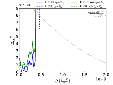
We see in the left panel of Fig. 7 that only a small contribution to $(g-2)_{\mu}$ is possible in sub-GUT models, the profile likelihood functions with and without the LHC 13-TeV data and $(g-2)_{\mu}$ being all quite similar. This is because in the sub-GUT model with low $M_{\rm in}$ the LHC searches for strongly-interacting sparticles constrain the $\tilde{\mu}$ mass more strongly than in the GUT-scale CMSSM. The dotted line shows the $\Delta\chi^{2}$ contribution due to our implementation of the $(g-2)_{\mu}$ constraint alone. We see that in all cases it contributes $\Delta\chi^{2}\gtrsim 9$ to the global fit.

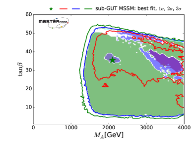
4.6 The $(M_{A},\tan\beta)$ Plane

The right panel of Fig. 7 shows the $(M_{A},\tan\beta)$ plane when the LHC 13-TeV data and the $(g-2)_{\mu}$ constraint are included in the fit. We see that $M_{A}\gtrsim 1.3\,\,\mathrm{TeV}$ at the 95% CL and that, whereas $\tan\beta\sim 5$ is allowed at the 95% CL. Larger values $\tan\beta\gtrsim 30$ are favoured at the 68% CL, and the best-fit point has $\tan\beta\simeq 36$. (This increases to $\tan\beta\sim 45$ if either the LHC 13-TeV and/or $(g-2)_{\mu}$ constraint is dropped.) As in the previous two-dimensional projections of the sub-GUT parameter space, the 99.7% (3-$\sigma$) CL contour lies close to that for the 95% CL.

4.7 $\mathbf{B}$ Decay Observables

Figure 8: Left panel: One-dimensional profile likelihood function for ${\rm BR}(B_{s,d}\to\mu^{+}\mu^{-})$, where the dotted line shows the $\chi^{2}$ contribution due to the ${\rm BR}(B_{s,d}\to\mu^{+}\mu^{-})$ constraint alone. Right panel: Breakdown of the contributions to the global $\chi^{2}$ as functions of $M_{\rm in}$. The shadings correspond to the different classes of observables, as indicated in the legend.

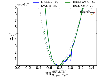
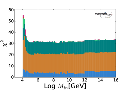
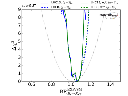
We see in the left panel of Fig. 8 that values of ${\rm BR}(B_{s,d}\to\mu^{+}\mu^{-})$ smaller than that in the SM are favoured. The sub-GUT models with $\mu>0$ that we have studied can accommodate comfortably the preference seen in the data (dotted line) for such a small value of ${\rm BR}(B_{s,d}\to\mu^{+}\mu^{-})$ , which is not the case in models such as the CMSSM that impose universal boundary conditions on the soft supersymmetry-breaking parameters at the GUT scale, if $\mu>0$. The right panel of Fig. 8 shows how the contributions of the flavour (blue shading) and other observables to the global likelihood function depend on $M_{\rm in}$ for values between $10^{4}$ and $10^{16}\,\,\mathrm{GeV}$. This variation in the flavour contribution (which is dominated by ${\rm BR}(B_{s,d}\to\mu^{+}\mu^{-})$) is largely responsible for the sub-GUT preference for $M_{\rm in}<M_{\rm GUT}$ seen in the top left panel of Fig. 1. Values of $M_{\rm in}\in(10^{5},10^{12})\,\,\mathrm{GeV}$ can accommodate very well the experimental value of ${\rm BR}(B_{s,d}\to\mu^{+}\mu^{-})$.

This preference is made possible by the different RGE running in the sub-GUT model, which can change the sign of the product $A_{t}\mu$ that controls the relative signs of the SM and SUSY contributions to the $B_{s,d}\to\mu^{+}\mu^{-}$ decay amplitudes, permitting negative interference that reduces ${\rm BR}(B_{s,d}\to\mu^{+}\mu^{-})$. As already discussed, the reduction in ${\rm BR}(B_{s,d}\to\mu^{+}\mu^{-})$ and the global $\chi^{2}$ function for $10^{8}\,\,\mathrm{GeV}\lesssim M_{\rm in}\lesssim 10^{12}\,\,\mathrm{GeV}$ is associated with the blue 68% CL regions with $M_{\rm in}\lesssim 10^{12}\,\,\mathrm{GeV}$ seen in the middle panels of Fig. 1. On the other hand, we see in Fig. 9 that sub-GUT models favour values of BR($b\to s\gamma$) that are close to the SM value.

The contributions to the global $\chi^{2}$ function of other classes of observables as functions of $M_{\rm in}$ are also exhibited in the right panel of Fig. 8. In addition to the aforementioned reduction in the flavour contribution when $M_{\rm in}\lesssim 10^{12}\,\,\mathrm{GeV}$ (blue shading), there is a coincident (but smaller) increase in the contribution of the electroweak precision observables (orange shading) related to tension in the electroweak symmetry-breaking conditions. The other contributions to the global $\chi^{2}$ function, namely the nuisance parameters (red shading), Higgs mass (light green), $(g-2)_{\mu}$ (teal) and DM (red), vary smoothly for $M_{\rm in}\sim 10^{12}\,\,\mathrm{GeV}$.

Figure 9: One-dimensional profile likelihood function for BR($b\to s\gamma$), showing the experimental constraint as a dotted line.

4.8 Higgs Mass

Figure 10: One-dimensional profile likelihood function for $M_{h}$, where the dotted line shows the $\chi^{2}$ contribution due to the $(g-2)_{\mu}$ constraint alone.

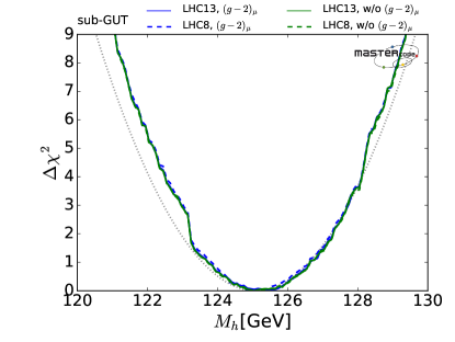
We see in Fig. 10 that the profile likelihood function for $M_{h}$ lies within the contribution of the direct experimental constraint convoluted with the uncertainty in the FeynHiggs calculation of $M_{h}$ (dotted line). We infer that there is no tension between the direct experimental measurement of $M_{h}$ and the other observables included in our global fit. We have also calculated (not shown) the branching ratios for Higgs decays into $\gamma\gamma$, $ZZ^{*}$ and $gg$ (used as a proxy for $gg\to h$ production), finding that they are expected to be very similar to their values in the SM, with 2-$\sigma$ ranges that lie well within the current experimental uncertainties.

4.9 Searches for Dark Matter Scattering

Figure 11: Left panel: Two-dimensional profile likelihood function for the nominal value of $\sigma^{\rm SI}_{p}$ calculated using the SSARD code [53] in the $(m_{\tilde{\chi}^{0}_{1}},\sigma^{\rm SI}_{p})$ plane, displaying also the upper limits established by the LUX [3], XENON1T [5] and PandaX-II Collaborations [6] shown as solid black, blue and green contours, respectively. The projected future 90% CL sensitivities of the LUX-Zeplin (LZ) [67] and XENON1T/nT [68] experiments are shown as dashed magenta and blue lines, respectively, and the neutrino background ‘floor’ [69] is shown as a dashed orange line with yellow shading below. Right panel: Two-dimensional profile likelihood function for the nominal value of $\sigma^{\rm SD}_{p}$ calculated using the SSARD code [53] in the $(m_{\tilde{\chi}^{0}_{1}},\sigma^{\rm SD}_{p})$ plane, showing also the upper limit established by the PICO Collaboration [4].We also show the indirect limits from the Icecube [56] and Super-Kamiokande [70] experiments, assuming $\tilde{\chi}^{0}_{1}\tilde{\chi}^{0}_{1}\to\tau^{+}\tau^{-}$ dominates, as well as the ‘floor’ for $\sigma^{\rm SD}_{p}$ calculated in [71].

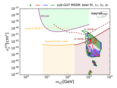
The left panel of Fig. 11 shows the nominal predictions for the spin-independent DM scattering cross-section $\sigma^{\rm SI}_{p}$ obtained using the SSARD code [53]. We caution that there are considerable uncertainties in the calculation of $\sigma^{\rm SI}_{p}$, which are taken into account in our global fit. Thus points with nominal values of $\sigma^{\rm SI}_{p}$ above the experimental limit may nevertheless lie within the 95% CL range for the global fit. We see that sub-GUT models favour a range of $\sigma^{\rm SI}_{p}$ close to the present limit from the LUX, XENON1T and PandaX-II experiments . Moreover, at the 95% CL, the nominal sub-GUT predictions for $\sigma^{\rm SI}_{p}$ are within the projected reaches of the LZ and XENON1/nT experiments. However, they are subject to the considerable uncertainty in the $\sigma^{\rm SI}_{p}$ matrix element, and might even fall below the neutrino ‘floor’ shown as a dashed orange line in [69].

We see in the right panel of Fig. 11 that the sub-GUT predictions for the spin-dependent DM scattering cross-section $\sigma^{\rm SD}_{p}$ lie somewhat below the present upper limit from the PICO direct DM search experiment. Spin-dependent DM scattering is also probed by indirect searches for neutrinos produced by the annihilations of neutralinos trapped inside the Sun after scattering on protons in its interior. If the neutralinos annihilate into $\tau^{+}\tau^{-}$, the IceCube experiment sets the strongest such indirect limit [56], and we also show the constraint from Super-Kamiokande [70]. These constraints are currently not sensitive enough to cut into the range of the $(m_{\tilde{\chi}^{0}_{1}},\sigma^{\rm SD}_{p})$ plane allowed in our global fit. We also show the neutrino ‘floor’ for $\sigma^{\rm SD}_{p}$, taken from [71]: wee that values of $\sigma^{\rm SD}_{p}$ below this floor are quite possible in the sub-GUT model.

5 Impacts of the LHC 13-TeV and New Direct Detection Constraints

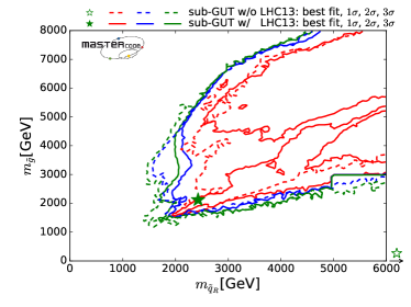
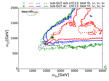
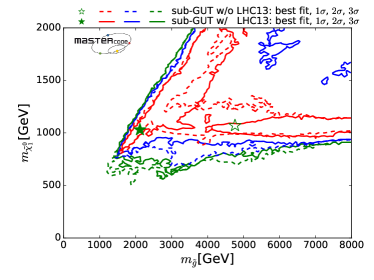
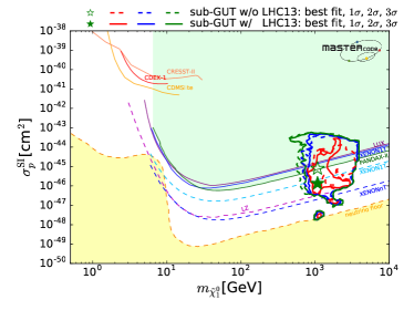
We show in Fig. 12 some two-dimensional projections of the regions of sub-GUT MSSM parameters favoured at the 68% (red lines), 95% (blue lines) and 99.7% CL (green lines), comparing the results of fits including the LHC 13-TeV data and recent direct searches for spin-independent dark matter scattering (solid lines) and discarding them (dashed lines). The upper left panel shows the $(m_{\tilde{q}_{R}},m_{\tilde{g}})$ plane, the upper right plane shows the $(m_{\tilde{q}_{R}},m_{\tilde{\chi}^{0}_{1}})$ plane, the lower left plane shows the $(m_{\tilde{g}},m_{\tilde{\chi}^{0}_{1}})$ plane, and the lower right panel shows the $(m_{\tilde{\chi}^{0}_{1}},\sigma^{\rm SI}_{p})$ plane. We see that in the upper panels that the new data restrict the favoured parameter space for $m_{\tilde{q}_{R}}\sim 2\,\,\mathrm{TeV}$, the two left panels show a restriction for $m_{\tilde{g}}\sim 1.3\,\,\mathrm{TeV}$, and the right and lower panels show that the new data also restrict the range of $m_{\tilde{\chi}^{0}_{1}}$ to $\gtrsim 800\,\,\mathrm{GeV}$. However, the lower right panel does not show any new restriction on the range of possible values of $\sigma^{\rm SI}_{p}$.

Figure 12: Two-dimensional projections of the global likelihood function for the sub-GUT MSSM in the $(m_{\tilde{q}_{R}},m_{\tilde{g}})$ plane (upper left panel), the $(m_{\tilde{q}_{R}},m_{\tilde{\chi}^{0}_{1}})$ plane (upper right panel), the $(m_{\tilde{g}},m_{\tilde{\chi}^{0}_{1}})$ plane (lower left panel), and the $(m_{\tilde{\chi}^{0}_{1}},\sigma^{\rm SI}_{p})$ plane (lower right panel). In each panel we compare the projections of the sub-GUT parameter regions favoured at the 68% (red lines), 95% (blue lines) and 99.7% CL (green lines) in global fits with the LHC 13-TeV data and results from LUX, XENON1T, and PandaX-II [3, 5, 6] (solid lines), and without them (dashed lines).

6 Best-Fit Points, Spectra and Decay Modes

The values of the input parameters at the best-fit points with and without the $(g-2)_{\mu}$ and LHC 13-TeV constraints have been shown in Table 2. The best fits have $M_{\rm in}$ between $1.6\times 10^{5}$ and $4.1\times 10^{8}\,\,\mathrm{GeV}$, and we note that the input parameters are rather insensitive to the inclusion of the 13-TeV data when $(g-2)_{\mu}$ is dropped. Table 4 displays the mass spectra obtained as outputs at the best-fit point including the 13-TeV data (quoted to 3 significant figures) and including (left column) or dropping (right column) the $(g-2)_{\mu}$ constraint. As could be expected, the sparticle masses are generally heavier when $(g-2)_{\mu}$ is dropped. However, the differences are small in the cases of the $\tilde{\chi}^{0}_{1},\tilde{\chi}^{0}_{2}$ and $\tilde{\chi}^{\pm}_{1}$, being generally $<10\,\,\mathrm{GeV}$. We also give in the next-to-last line of Table 4 the values of the global $\chi^{2}$ function at these best-fit points, dropping the HiggsSignals contributions, as was done previously [21, 33] to avoid biasing the analysis.

	With $(g-2)_{\mu}$	Without $(g-2)_{\mu}$
$M_{H,A,H^{+}}$	2060	2220
$\tilde{d}_{L},\tilde{u}_{L},\tilde{s}_{L},\tilde{c}_{L}$	2510	5050
$\tilde{d}_{R},\tilde{u}_{R},\tilde{s}_{R},\tilde{c}_{R}$	2450	4835
$\tilde{b}_{1}$	1830	4100
$\tilde{b}_{2}$	2190	4210
$\tilde{t}_{1}$	1130	3430
$\tilde{t}_{2}$	1850	4150
$\tilde{e}_{L},\tilde{\nu}_{e_{L}},\tilde{\mu}_{L},\tilde{\nu}_{\mu_{L}}$	2040	3740
$\tilde{e}_{R},\tilde{\mu}_{R}$	1980	3510
$\tilde{\tau}_{1}$	1380	2740
$\tilde{\tau}_{2}$	1780	3390
$\tilde{\nu}_{\tau_{L}}$	1770	3390
$\tilde{g}$	2120	7240
$m_{\tilde{\chi}_{1}^{0}}$	1040	1060
$m_{\tilde{\chi}_{2}^{0}}$	1270	1060
$m_{\tilde{\chi}_{3}^{0}}$	1740	6010
$m_{\tilde{\chi}_{4}^{0}}$	1740	6300
$m_{\tilde{\chi}_{1}^{\pm}}$	1270	1060
$m_{\tilde{\chi}_{2}^{\pm}}$	1740	6310
$\chi^{2}$ without
HiggsSignals	28.86	18.02
Number of d.o.f.	24	23
p-value	23%	76%

Table 4: The spectra at the best-fit points including the LHC 13-TeV data and including (left column) or dropping (right column) the $(g-2)_{\mu}$ constraint. The masses are quoted in GeV. The three bottom lines give the values of the $\chi^{2}$ function dropping HiggsSignals, the numbers of degrees of freedom (d.o.f.) and the corresponding p-values.

The contributions of different observables to the global likelihood function at the best-fit points including LHC13 data are shown in Fig. 13. We compare the contributions when $(g-2)_{\mu}$ is included (pink histograms) and without $(g-2)_{\mu}$ (blue histograms). We note, in particular, that the contribution of ${\rm BR}(B_{s,d}\to\mu^{+}\mu^{-})$ is very small in both cases, which is a distinctive feature of sub-GUT models.

\begin{overpic}[scale={0.6}]{sub_171017_breakdown_compared.pdf} \put(25.0,85.0){\includegraphics[width=43.36464pt]{mastercode-logo.png}} \end{overpic}

Figure 13: Contributions to the global $\chi^{2}$ function at the best-fit points found in our sub-GUT analysis including LHC 13-TeV data, in the cases with and without the $(g-2)_{\mu}$ constraint (pink and blue histograms, respectively).

The last line of Table 4 shows the p-values for the best fits with and without $(g-2)_{\mu}$, which were calculated as follows. In the case with (without) $(g-2)_{\mu}$, setting aside HiggsSignals so as to avoid biasing the analysis [21, 33], the number of constraints making non-zero contributions to the global $\chi^{2}$ function (not including nuisance parameters) is 29 (28), and the number of free parameters is 5 in each case. Hence the numbers of degrees of freedom are 24 (23) in the two cases. The values of the total $\chi^{2}$ function at the best-fit points, dropping the HiggsSignals contribution, are 28.9 (18.0) and the corresponding p-values are 23% (76%). The qualities of the global fits with and without $(g-2)_{\mu}$ are therefore both good. and the fit including $(g-2)_{\mu}$ is not poor enough to reject this fit hypothesis.

The spectra for the best fits are displayed graphically in Fig. 14, including the $(g-2)_{\mu}$ constraint (upper panel) and dropping it (lower panel). Also shown are the decay modes with branching ratios $>5\%$, as dashed lines whose intensities increase with the branching ratios. The heavy Higgs bosons decay predominantly to SM final states, hence no dashed lines are shown. We see that in both cases the squarks and gluino are probably too heavy to be discovered at the LHC, and the sleptons are too heavy to be discovered at any planned $e^{+}e^{-}$ collider. The best prospects for sparticle discovery may be for $\tilde{\chi}^{\pm}_{1}$ and $\tilde{\chi}^{0}_{2}$ production at CLIC running at $E_{\rm CM}\gtrsim 2\,\,\mathrm{TeV}$ [75].

\begin{overpic}[scale={0.6}]{sub_171017_decays.pdf} \put(15.0,55.0){\includegraphics[width=43.36464pt]{mastercode-logo.png}} \end{overpic}

\begin{overpic}[scale={0.6}]{sub_171017_decays_wo_gm2.pdf} \put(15.0,55.0){\includegraphics[width=43.36464pt]{mastercode-logo.png}} \end{overpic}

Figure 14: The spectra of Higgs bosons and sparticles at the best-fit points in the sub-GUT model including LHC 13-TeV data, including the $(g-2)_{\mu}$ constraint (upper panel) and dropping it (lower panel), with dashed lines indicating the decay modes with branching ratios $>5\%$. These plots were made using PySLHA [76].

The global likelihood function is quite flat at large sparticle masses, and very different spectra are consistent with the data, within the current uncertainties. The 68 and 95% CL ranges of Higgs and sparticle masses are displayed in Fig. 15 as orange and yellow bands, respectively, with the best-fit values indicated by blue lines. The upper panel is for a fit including the $(g-2)_{\mu}$ constraint, which is dropped in the lower panel. At the 68% CL there are possibilities for squark and gluino discovery at the LHC and the $\tilde{\tau}_{1},{\tilde{\mu}_{R}}$ and ${\tilde{e}_{R}}$ become potentially discoverable at CLIC if it operates at $E_{\rm CM}=3\,\,\mathrm{TeV}$ [75].

\begin{overpic}[width=433.62pt]{sub_171017_mass-spectrum.pdf} \put(77.0,7.0){\includegraphics[width=43.36464pt]{mastercode-logo.png}} \end{overpic}

\begin{overpic}[width=433.62pt]{sub_171017_mass-spectrum_wo_gm2.pdf} \put(77.0,7.0){\includegraphics[width=43.36464pt]{mastercode-logo.png}} \end{overpic}

Figure 15: The spectra in the sub-GUT model including LHC 13-TeV data, with (upper panel) and without (lower panel) the $(g-2)_{\mu}$ constraint, displaying the best-fit values as blue lines, the 68% CL ranges as orange bands, and the 95% CL ranges as yellow bands.

7 Summary and Perspectives

We have performed in this paper a frequentist analysis of sub-GUT models in which soft supersymmetry-breaking parameters are assumed to be universal at some input scale $M_{\rm in}<M_{\rm GUT}$. The best-fit input parameters with and without $(g-2)_{\mu}$ and the LHC 13-TeV data are shown in Table 2. The physical sparticle masses including the LHC data, with and without $(g-2)_{\mu}$, are shown in Table 4 and in Fig. 14, where decay patterns are also indicated. As seen in the bottom line of Table 4, the p-values for the fits with and without $(g-2)_{\mu}$ are $\simeq 23$% and $76$%, respectively.

Compared to the best fits with $M_{\rm in}=M_{\rm GUT}$, we have found that the minimum value of the global $\chi^{2}$ function may be reduced by $\Delta\chi^{2}\sim 2$ in the sub-GUT model, with the exact amount depending whether the $(g-2)_{\mu}$ constraint and/or LHC13 data are included in the fit. Whether these observables are included, or not, the global $\chi^{2}$ minimum occurs for $M_{\rm in}\sim 10^{7}\,\,\mathrm{GeV}$, and is due to the sub-GUT model’s ability to provide a better fit to the measured value of ${\rm BR}(B_{s,d}\to\mu^{+}\mu^{-})$ than in the CMSSM. Although intriguing, this improvement in the fit quality is not very significant, but it will be interesting to monitor how the experimental measurement of ${\rm BR}(B_{s,d}\to\mu^{+}\mu^{-})$ evolves.

In all the scenarios studied (with/without $(g-2)_{\mu}$ and/or LHC13), the profile likelihood function for $m_{\tilde{g}}$ ($m_{\tilde{q}}$) varies by $\lesssim 1$ for $m_{\tilde{g}}\gtrsim 1.9\,\,\mathrm{TeV}$ ($m_{\tilde{q}}\gtrsim 2.2\,\,\mathrm{TeV}$). The corresponding slowly-varying ranges of $\chi^{2}$ for $m_{\tilde{t}_{1}}$ ($m_{\tilde{b}_{1}}$) start at $\sim 1\,\,\mathrm{TeV}$ ($\sim 1.6\,\,\mathrm{TeV}$), respectively. On the other hand, we find a more marked preference for $m_{\tilde{\chi}^{0}_{1}}\sim 1\,\,\mathrm{TeV}$, with the $\tilde{\chi}^{\pm}_{1}$ and $\tilde{\chi}^{0}_{2}$ being slightly heavier and large mass values being disfavoured at the $\Delta\chi^{2}\sim 3$ level. The best-fit point is in a region where rapid annihilation via $H/A$ poles is hybridized with stop coannihilation, with chargino coannihilation and stau coannihilation also playing roles in both the 68 and 95% CL regions. Within the 95% CL region, the chargino lifetime may exceed $10^{-12}$ s, and the stau lifetime may be as long as one second, motivating continued searches for long-lived sparticles at the LHC.

Taking the LHC13 constraints into account, we find that the spin-independent DM cross-section, $\sigma^{\rm SI}_{p}$, may be just below the present upper limits from the LUX, XENON1T and PandaX-II experiments, and within the reaches of the planned XENONnT and LZ experiments. On the other hand, the spin-dependent DM cross-section, $\sigma^{\rm SD}_{p}$, may be between some 2 and 5 orders of magnitude below the current upper limit from the PICO experiment.

Within the sub-GUT framework, therefore, we find interesting perspectives for LHC searches for strongly-interacting sparticles via the conventional missing-energy signature. Future $/E_{T}$ searches for electroweakly-interacting sparticles and for long-lived massive charged particles may also have interesting prospects. The best-fit region of parameter space accommodates the observed deviation of ${\rm BR}(B_{s,d}\to\mu^{+}\mu^{-})$ from its value in the SM, and it will be interesting to see further improvement in the precision of this measurement. A future $e^{+}e^{-}$ collider with centre-of-mass energy above 2 TeV, such as CLIC [75], would have interesting perspectives for discovering and measuring the properties of electroweakly-interacting sparticles. There are also interesting perspectives for direct DM searches via spin-independent scattering.

References

- [1] For a compendium of CMS searches for supersymmetry, see https://twiki.cern.ch/twiki/bin/view/ CMSPublic/PhysicsResultsSUS.
- [2] For a compendium of ATLAS searches for supersymmetry, see https://twiki.cern.ch/twiki/bin/view/ AtlasPublic/SupersymmetryPublicResults.
- [3] D. S. Akerib et al. [LUX Collaboration], Phys. Rev. Lett. 118 (2017) no.2, 021303 [arXiv:1608.07648 [astro-ph.CO]].
- [4] C. Amole et al. [PICO Collaboration], arXiv:1702.07666 [astro-ph.CO].
- [5] E. Aprile et al. [XENON Collaboration], arXiv:1705.06655 [astro-ph.CO].
- [6] X. Cui et al. [PandaX-II Collaboration], arXiv:1708.06917 [hep-ex], which updates A. Tan et al. [PandaX-II Collaboration], Phys. Rev. Lett. 117 (2016) no. 12, 121303 [arXiv:1607.07400 [hep-ex]].
- [7] H. Goldberg, Phys. Rev. Lett. 50 (1983) 1419; J. Ellis, J. Hagelin, D. Nanopoulos, K. Olive and M. Srednicki, Nucl. Phys. B 238 (1984) 453.
- [8] O. Buchmueller et al., Eur. Phys. J. C 72 (2012) 1878 [arXiv:1110.3568 [hep-ph]]; Eur. Phys. J. C 72 (2012) 2243 [arXiv:1207.7315]; Eur. Phys. J. C 74 (2014) 2809 [arXiv:1312.5233 [hep-ph]].
- [9] O. Buchmueller et al., Eur. Phys. J. C 74 (2014) 2922 [arXiv:1312.5250 [hep-ph]].
- [10] P. Bechtle et al., Eur. Phys. J. C 76 (2016) no.2, 96 [arXiv:1508.05951 [hep-ph]].
- [11] P. Athron et al. [GAMBIT Collaboration], arXiv:1705.07935 [hep-ph].
- [12] O. Buchmueller et al., Eur. Phys. J. C 74 (2014) 12, 3212 [arXiv:1408.4060 [hep-ph]].
- [13] See, for example, C. F. Berger, J. S. Gainer, J. L. Hewett and T. G. Rizzo, JHEP 0902, 023 (2009) [arXiv:0812.0980 [hep-ph]]; S. S. AbdusSalam, B. C. Allanach, F. Quevedo, F. Feroz and M. Hobson, Phys. Rev. D 81, 095012 (2010) [arXiv:0904.2548 [hep-ph]]; J. A. Conley, J. S. Gainer, J. L. Hewett, M. P. Le and T. G. Rizzo, Eur. Phys. J. C 71, 1697 (2011) [arXiv:1009.2539 [hep-ph]]; J. A. Conley, J. S. Gainer, J. L. Hewett, M. P. Le and T. G. Rizzo, [arXiv:1103.1697 [hep-ph]]; S. S. AbdusSalam, et al., Eur. Phys. J. C 71 (2011) 1835 [arXiv:1109.3859 [hep-ph]]; S. Sekmen, S. Kraml, J. Lykken, F. Moortgat, S. Padhi, L. Pape, M. Pierini and H. B. Prosper et al., JHEP 1202 (2012) 075 [arXiv:1109.5119 [hep-ph]]; A. Arbey, M. Battaglia and F. Mahmoudi, Eur. Phys. J. C 72 (2012) 1847 [arXiv:1110.3726 [hep-ph]]; A. Arbey, M. Battaglia, A. Djouadi and F. Mahmoudi, Phys. Lett. B 720 (2013) 153 [arXiv:1211.4004 [hep-ph]]; M. W. Cahill-Rowley, J. L. Hewett, A. Ismail and T. G. Rizzo, Phys. Rev. D 88 (2013) 3, 035002 [arXiv:1211.1981 [hep-ph]].
- [14] K. J. de Vries et al., Eur. Phys. J. C 75 (2015) no.9, 422 [arXiv:1504.03260 [hep-ph]].
- [15] P. Athron et al. [GAMBIT Collaboration], arXiv:1705.07917 [hep-ph].
- [16] E. Bagnaschi et al., arXiv:1710.11091 [hep-ph].
- [17] J. Ellis, T. Falk, and K.A. Olive, Phys. Lett. B444 (1998) 367 [arXiv:hep-ph/9810360]; J. Ellis, T. Falk, K.A. Olive, and M. Srednicki, Astr. Part. Phys. 13 (2000) 181 [Erratum-ibid. 15 (2001) 413] [arXiv:hep-ph/9905481]; R. Arnowitt, B. Dutta and Y. Santoso, Nucl. Phys. B 606 (2001) 59 [arXiv:hep-ph/0102181]; M. E. Gómez, G. Lazarides and C. Pallis, Phys. Rev. D D61 (2000) 123512 [arXiv:hep-ph/9907261]; Phys. Lett. B487 (2000) 313 [arXiv:hep-ph/0004028]; Nucl. Phys. B B638 (2002) 165 [arXiv:hep-ph/0203131]; T. Nihei, L. Roszkowski and R. Ruiz de Austri, JHEP 0207 (2002) 024 [arXiv:hep-ph/0206266].
- [18] M. Citron, J. Ellis, F. Luo, J. Marrouche, K. A. Olive and K. J. de Vries, Phys. Rev. D 87 (2013) no.3, 036012 [arXiv:1212.2886 [hep-ph]].
- [19] C. Boehm, A. Djouadi and M. Drees, Phys. Rev. D 62, 035012 (2000) [arXiv:hep-ph/9911496]; J. R. Ellis, K. A. Olive and Y. Santoso, Astropart. Phys. 18, 395 (2003) [arXiv:hep-ph/0112113]; J. L. Diaz-Cruz, J. R. Ellis, K. A. Olive and Y. Santoso, JHEP 0705, 003 (2007) [arXiv:hep-ph/0701229]; I. Gogoladze, S. Raza and Q. Shafi, Phys. Lett. B 706, 345 (2012) [arXiv:1104.3566 [hep-ph]]; M. A. Ajaib, T. Li and Q. Shafi, Phys. Rev. D 85, 055021 (2012) [arXiv:1111.4467 [hep-ph]]; J. Harz, B. Herrmann, M. Klasen, K. Kovarik and Q. L. Boulc’h, Phys. Rev. D 87 (2013) 5, 054031 [arXiv:1212.5241]; J. Ellis, K. A. Olive and J. Zheng, Eur. Phys. J. C 74 (2014) 2947 [arXiv:1404.5571 [hep-ph]]; J. Harz, B. Herrmann, M. Klasen and K. Kovarik, Phys. Rev. D 91 (2015) 3, 034028 [arXiv:1409.2898 [hep-ph]]; A. Ibarra, A. Pierce, N. R. Shah and S. Vogl, Phys. Rev. D 91, no. 9, 095018 (2015) [arXiv:1501.03164 [hep-ph]]; A. Pierce, N. R. Shah and S. Vogl, arXiv:1706.01911 [hep-ph].
- [20] S. Mizuta and M. Yamaguchi, Phys. Lett. B 298 (1993) 120 [arXiv:hep-ph/9208251]; J. Edsjo and P. Gondolo, Phys. Rev. D 56, 1879 (1997) [hep-ph/9704361]; H. Baer, C. Balazs and A. Belyaev, JHEP 0203, 042 (2002) [hep-ph/0202076]; A. Birkedal-Hansen and E. h. Jeong, JHEP 0302, 047 (2003) [hep-ph/0210041]; J. Edsjo, M. Schelke, P. Ullio and P. Gondolo, JCAP 0304, 001 (2003) [hep-ph/0301106].
- [21] E. Bagnaschi et al., Eur. Phys. J. C 77 (2017) no.2, 104 [arXiv:1610.10084 [hep-ph]].
- [22] S. Profumo and C. E. Yaguna, Phys. Rev. D 69, 115009 (2004) [hep-ph/0402208]; D. Feldman, Z. Liu and P. Nath, Phys. Rev. D 80, 015007 (2009) [arXiv:0905.1148 [hep-ph]]; N. Chen, D. Feldman, Z. Liu, P. Nath and G. Peim, Phys. Rev. D 83, 035005 (2011) [arXiv:1011.1246 [hep-ph]]; I. Gogoladze, R. Khalid and Q. Shafi, Phys. Rev. D 79, 115004 (2009) [arXiv:0903.5204 [hep-ph]]; I. Gogoladze, R. Khalid and Q. Shafi, Phys. Rev. D 80, 095016 (2009) [arXiv:0908.0731 [hep-ph]]; M. Adeel Ajaib, T. Li, Q. Shafi and K. Wang, JHEP 1101, 028 (2011) [arXiv:1011.5518 [hep-ph]]; K. Harigaya, M. Ibe and T. T. Yanagida, JHEP 1312, 016 (2013) [arXiv:1310.0643 [hep-ph]]; K. Harigaya, K. Kaneta and S. Matsumoto, Phys. Rev. D 89, no. 11, 115021 (2014) [arXiv:1403.0715 [hep-ph]]; S. Raza, Q. Shafi and C. S. Ün, Phys. Rev. D 92, no. 5, 055010 (2015) [arXiv:1412.7672 [hep-ph]]; J. L. Evans and K. A. Olive, Phys. Rev. D 90, no. 11, 115020 (2014) [arXiv:1408.5102 [hep-ph]]; A. De Simone, G. F. Giudice and A. Strumia, JHEP 1406, 081 (2014) [arXiv:1402.6287 [hep-ph]]; JHEP 1408, 161 (2014) [arXiv:1404.0682 [hep-ph]].
- [23] J. Ellis, F. Luo and K. A. Olive, JHEP 1509 (2015) 127 [arXiv:1503.07142 [hep-ph]]; J. Ellis, J. L. Evans, F. Luo and K. A. Olive, JHEP 1602 (2016) 071 [arXiv:1510.03498 [hep-ph]].
- [24] J. R. Ellis, K. A. Olive and P. Sandick, Phys. Lett. B 642 (2006) 389 [hep-ph/0607002], JHEP 0706 (2007) 079 [arXiv:0704.3446 [hep-ph]] and JHEP 0808 (2008) 013 [arXiv:0801.1651 [hep-ph]].
- [25] J. Ellis, F. Luo, K. A. Olive and P. Sandick, Eur. Phys. J. C 73, no. 4, 2403 (2013) [arXiv:1212.4476 [hep-ph]]; J. Ellis, J. L. Evans, F. Luo, N. Nagata, K. A. Olive and P. Sandick, Eur. Phys. J. C 76, no. 1, 8 (2016) [arXiv:1509.08838 [hep-ph]].
- [26] H. Itoh, N. Okada and T. Yamashita, arXiv:hep-ph/0606156.
- [27] C. Csaki, in M. Shifman et al. (eds.), From fields to strings, vol. 2, pp967-1060, [hep-ph/0404096]; K. Choi, A. Falkowski, H. P. Nilles and M. Olechowski, Nucl. Phys. B 718 (2005) 113 [arXiv:hep-th/0503216]; K. Choi, K. S. Jeong and K. i. Okumura, JHEP 0509 (2005) 039 [arXiv:hep-ph/0504037]; M. Endo, M. Yamaguchi and K. Yoshioka, Phys. Rev. D 72 (2005) 015004 [arXiv:hep-ph/0504036]; A. Falkowski, O. Lebedev and Y. Mambrini, JHEP 0511 (2005) 034 [arXiv:hep-ph/0507110]; R. Kitano and Y. Nomura, Phys. Lett. B 631 (2005) 58 [arXiv:hep-ph/0509039]; R. Kitano and Y. Nomura, Phys. Rev. D 73 (2006) 095004 [arXiv:hep-ph/0602096]; A. Pierce and J. Thaler, JHEP 0609 (2006) 017 [arXiv:hep-ph/0604192]; K. Kawagoe and M. M. Nojiri, [arXiv:hep-ph/0606104]; H. Baer, E.-K. Park, X. Tata and T. T. Wang, JHEP 0608 (2006) 041 [arXiv:hep-ph/0604253]; K. Choi, K. Y. Lee, Y. Shimizu, Y. G. Kim and K. i. Okumura, JCAP 0612 (2006) 017 [arXiv:hep-ph/0609132]; O. Lebedev, V. Lowen, Y. Mambrini, H. P. Nilles and M. Ratz, JHEP 0702 (2007) 063 [arXiv:hep-ph/0612035].
- [28] S. Kachru, R. Kallosh, A. D. Linde and S. P. Trivedi, Phys. Rev. D 68, 046005 (2003) [hep-th/0301240].
- [29] M. Dine and D. MacIntire, Phys. Rev. D 46, 2594 (1992) [hep-ph/9205227]; L. Randall and R. Sundrum, Nucl. Phys. B 557, 79 (1999) [arXiv:hep-th/9810155]; G. F. Giudice, M. A. Luty, H. Murayama and R. Rattazzi, JHEP 9812, 027 (1998) [arXiv:hep-ph/9810442]; A. Pomarol and R. Rattazzi, JHEP 9905, 013 (1999) [hep-ph/9903448]; J. A. Bagger, T. Moroi and E. Poppitz, JHEP 0004, 009 (2000) [arXiv:hep-th/9911029]; P. Binetruy, M. K. Gaillard and B. D. Nelson, Nucl. Phys. B 604, 32 (2001) [arXiv:hep-ph/0011081].
- [30] G. Bennett et al. [The Muon g-2 Collaboration], Phys. Rev. Lett. 92 (2004) 161802, [arXiv:hep-ex/0401008]; and Phys. Rev. D 73 (2006) 072003 [arXiv:hep-ex/0602035].
- [31] D. Stockinger, J. Phys. G 34 (2007) R45 [arXiv:hep-ph/0609168]; J. Miller, E. de Rafael and B. Roberts, Rept. Prog. Phys. 70 (2007) 795 [arXiv:hep-ph/0703049]; J. Prades, E. de Rafael and A. Vainshtein, arXiv:0901.0306 [hep-ph]; F. Jegerlehner and A. Nyffeler, Phys. Rept. 477, 1 (2009) [arXiv:0902.3360 [hep-ph]]; M. Davier, A. Hoecker, B. Malaescu, C. Z. Yuan and Z. Zhang, Eur. Phys. J. C 66, 1 (2010) [arXiv:0908.4300 [hep-ph]]. J. Prades, Acta Phys. Polon. Supp. 3, 75 (2010) [arXiv:0909.2546 [hep-ph]]; T. Teubner, K. Hagiwara, R. Liao, A. D. Martin and D. Nomura, arXiv:1001.5401 [hep-ph]; M. Davier, A. Hoecker, B. Malaescu and Z. Zhang, Eur. Phys. J. C 71 (2011) 1515 [arXiv:1010.4180 [hep-ph]].
- [32] E. A. Bagnaschi et al., Eur. Phys. J. C 75 (2015) 500 [arXiv:1508.01173 [hep-ph]].
- [33] E. Bagnaschi et al., Eur. Phys. J. C 77 (2017) no.4, 268 [arXiv:1612.05210 [hep-ph]].
- [34] K. J. de Vries, PhD thesis Global Fits of Supersymmetric Models after LHC Run 1 (2015), available on the MasterCode website: http://cern.ch/mastercode/.
- [35] For more information and updates, please see http://cern.ch/mastercode/.
- [36] A. M. Sirunyan et al. [CMS Collaboration], arXiv:1705.04650 [hep-ex].
- [37] A. M. Sirunyan et al. [CMS Collaboration], arXiv:1705.04673 [hep-ex].
- [38] A. M. Sirunyan et al. [CMS Collaboration], arXiv:1709.05406 [hep-ex].
- [39] V. Khachatryan et al. [CMS Collaboration], Eur. Phys. J. C 75 (2015) no.7, 325 [arXiv:1502.02522 [hep-ex]].
- [40] CMS Collaboration, CMS-PAS-EXO-16-036.
- [41] V. Khachatryan et al. [CMS and LHCb Collaborations], Nature 522 (2015) 68 [arXiv:1411.4413 [hep-ex]]
- [42] M. Aaboud et al. [ATLAS Collaboration], Eur. Phys. J. C 76 (2016) no.9, 513 [arXiv:1604.04263 [hep-ex]].
- [43] R. Aaij et al. [LHCb Collaboration], Phys. Rev. Lett. 118 (2017) no.19, 191801 [arXiv:1703.05747 [hep-ex]].
- [44] D. S. Akerib et al. [LZ Collaboration], arXiv:1509.02910 [physics.ins-det].
- [45] E. Aprile et al. [XENON Collaboration], arXiv:1708.07051 [astro-ph.IM].
-
[46]
G. Aad et al. [ATLAS and CMS Collaborations],
JHEP 1608 (2016) 045
[arXiv:1606.02266 [hep-ex]]. - [47] P. Bechtle, S. Heinemeyer, O. Stål, T. Stefaniak and G. Weiglein, Eur. Phys. J. C 74 (2014) 2, 2711 [arXiv:1305.1933 [hep-ph]]; JHEP 1411 (2014) 039 [arXiv:1403.1582 [hep-ph]].
- [48] P. Bechtle, O. Brein, S. Heinemeyer, G. Weiglein and K. E. Williams, Comput. Phys. Commun. 181 (2010) 138 [arXiv:0811.4169 [hep-ph]], Comput. Phys. Commun. 182 (2011) 2605 [arXiv:1102.1898 [hep-ph]]; P. Bechtle et al., Eur. Phys. J. C 74 (2014) 3, 2693 [arXiv:1311.0055 [hep-ph]]; P. Bechtle, S. Heinemeyer, O. Stål, T. Stefaniak and G. Weiglein, Eur. Phys. J. C 75 (2015) no.9, 421 [arXiv:1507.06706 [hep-ph]].
[49]
ATLAS Collaboration,
http://cds.cern.ch/record/2273866/ files/ATLAS-CONF-2017-050.pdf. - [50] P. A. R. Ade et al. [Planck Collaboration], Astron. Astrophys. 594 (2016) A13 [arXiv:1502.01589 [astro-ph.CO]].
- [51] G. Belanger, F. Boudjema, A. Pukhov and A. Semenov, Comput. Phys. Commun. 185 (2014) 960 [arXiv:1305.0237 [hep-ph]], and references therein.
- [52] J. R. Ellis, A. Ferstl and K. A. Olive, Phys. Lett. B 481, 304 (2000) [hep-ph/0001005]; J. R. Ellis, K. A. Olive, Y. Santoso and V. C. Spanos, Phys. Rev. D 71, 095007 (2005) [hep-ph/0502001]; J. R. Ellis, K. A. Olive and C. Savage, Phys. Rev. D 77 (2008) 065026 [arXiv:0801.3656 [hep-ph]].
- [53] Information about this code is available from K. A. Olive: it contains important contributions from J. Evans, T. Falk, A. Ferstl, G. Ganis, F. Luo, A. Mustafayev, J. McDonald, F. Luo, K. A. Olive, P. Sandick, Y. Santoso, C. Savage, V. Spanos and M. Srednicki.
- [54] X. Z. Ling, X. L. Ren and L. S. Geng, arXiv:1710.07164 [hep-ph].
- [55] J. M. Alarcon, J. Martin Camalich and J. A. Oller, Phys. Rev. D 85 (2012) 051503 [arXiv:1110.3797 [hep-ph]]; J. M. Alarcon, L. S. Geng, J. Martin Camalich and J. A. Oller, Phys. Lett. B 730 (2014) 342 [arXiv:1209.2870 [hep-ph]].
- [56] M. G. Aartsen et al. [IceCube Collaboration], Eur. Phys. J. C 77 (2017) no.3, 146 [arXiv:1612.05949 [astro-ph.HE]].
- [57] M. Papucci, K. Sakurai, A. Weiler and L. Zeune, Eur. Phys. J. C 74 (2014) no.11, 3163 [arXiv:1402.0492 [hep-ph]].
- [58] B. C. Allanach, Comput. Phys. Commun. 143 (2002) 305 [arXiv:hep-ph/0104145].
- [59] F. Feroz and M.P. Hobson, Mon. Not. Roy. Astron. Soc. 384 (2008) 449 [arXiv:0704.3704 [astro-ph]]. F. Feroz, M.P. Hobson and M. Bridges, Mon. Not. Roy. Astron. Soc. 398 (2009) 1601-1614 [arXiv:0809.3437 [astro-ph]]. F. Feroz, M.P. Hobson, E. Cameron and A.N. Pettitt, [arXiv:1306.2144 [astro-ph]].
- [60] P. Skands et al., JHEP 0407 (2004) 036 [arXiv:hep-ph/0311123]; B. Allanach et al., Comput. Phys. Commun. 180 (2009) 8 [arXiv:0801.0045 [hep-ph]].
- [61] S. Heinemeyer et al., JHEP 0608 (2006) 052 [arXiv:hep-ph/0604147]; S. Heinemeyer, W. Hollik, A. M. Weber and G. Weiglein, JHEP 0804 (2008) 039 [arXiv:0710.2972 [hep-ph]].
- [62] G. Isidori and P. Paradisi, Phys. Lett. B 639 (2006) 499 [arXiv:hep-ph/0605012]; G. Isidori, F. Mescia, P. Paradisi and D. Temes, Phys. Rev. D 75 (2007) 115019 [arXiv:hep-ph/0703035], and references therein.
- [63] F. Mahmoudi, Comput. Phys. Commun. 178 (2008) 745 [arXiv:0710.2067 [hep-ph]]; Comput. Phys. Commun. 180 (2009) 1579 [arXiv:0808.3144 [hep-ph]]; D. Eriksson, F. Mahmoudi and O. Stal, JHEP 0811 (2008) 035 [arXiv:0808.3551 [hep-ph]].
- [64] S. Heinemeyer, W. Hollik and G. Weiglein, Comput. Phys. Commun. 124 (2000) 76 [arXiv:hep-ph/9812320]; S. Heinemeyer, W. Hollik and G. Weiglein, Eur. Phys. J. C 9 (1999) 343 [arXiv:hep-ph/9812472]; G. Degrassi, S. Heinemeyer, W. Hollik, P. Slavich and G. Weiglein, Eur. Phys. J. C 28 (2003) 133 [arXiv:hep-ph/0212020]; M. Frank et al., JHEP 0702 (2007) 047 [arXiv:hep-ph/0611326]; T. Hahn, S. Heinemeyer, W. Hollik, H. Rzehak and G. Weiglein, Comput. Phys. Commun. 180 (2009) 1426; T. Hahn, S. Heinemeyer, W. Hollik, H. Rzehak and G. Weiglein, Phys. Rev. Lett. 112 (2014) 14, 141801 [arXiv:1312.4937 [hep-ph]]; H. Bahl and W. Hollik, Eur. Phys. J. C 76 (2016) 499 [arXiv:1608.01880 [hep-ph]]. See http://www.feynhiggs.de .
- [65] M. Muhlleitner, A. Djouadi and Y. Mambrini, Comput. Phys. Commun. 168 (2005) 46 [hep-ph/0311167].
- [66] J. D. Hunter, Computing In Science & Engineering, 9.3 (2007), pp90-95.
- [67] B. J. Mount et al., arXiv:1703.09144 [physics.ins-det].
- [68] E. Aprile et al. [XENON Collaboration], JCAP 1604 (2016) no.04, 027 doi:10.1088/1475-7516/2016/04/027 [arXiv:1512.07501 [physics.ins-det]].
- [69] J. Billard, L. Strigari and E. Figueroa-Feliciano, Phys. Rev. D 89, no. 2, 023524 (2014) [arXiv:1307.5458 [hep-ph]]; P. Cushman, C. Galbiati, D. N. McKinsey, H. Robertson, T. M. P. Tait, D. Bauer, A. Borgland and B. Cabrera et al., Snowmass Working Group Report: WIMP Dark Matter Direct Detection, arXiv:1310.8327 [hep-ex].
- [70] K. Choi et al. [Super-Kamiokande Collaboration], Phys. Rev. Lett. 114 (2015) no.14, 141301 doi:10.1103/PhysRevLett.114.141301 [arXiv:1503.04858 [hep-ex]].
- [71] K. C. Y. Ng, J. F. Beacom, A. H. G. Peter and C. Rott, arXiv:1703.10280 [astro-ph.HE].
- [72] G. Angloher et al. [CRESST Collaboration], Eur. Phys. J. C 76 (2016) no.1, 25 doi:10.1140/epjc/s10052-016-3877-3 [arXiv:1509.01515 [astro-ph.CO]].
- [73] R. Agnese et al. [SuperCDMS Collaboration], Phys. Rev. Lett. 116 (2016) no.7, 071301 doi:10.1103/PhysRevLett.116.071301 [arXiv:1509.02448 [astro-ph.CO]].
- [74] L. T. Yang et al. [CDEX Collaboration], arXiv:1710.06650 [hep-ex].
- [75] M. J. Boland et al. [CLIC and CLICdp Collaborations], arXiv:1608.07537 [physics.acc-ph].
- [76] A. Buckley, Eur. Phys. J. C 75, no. 10, 467 (2015) [arXiv:1305.4194 [hep-ph]].