Phase Diagram of Stability for Massive Scalars in Anti-de Sitter Spacetime

Abstract

We diagram the behavior of 5-dimensional anti-de Sitter spacetime against horizon formation in the gravitational collapse of a scalar field, treating the scalar field mass and width of initial data as free parameters, which we call the stability phase diagram. We find that the class of stable initial data becomes larger and shifts to smaller widths as the field mass increases. In addition to classifying initial data as stable or unstable, we identify two other classes based on nonperturbative behavior. The class of metastable initial data forms a horizon over longer time scales than suggested by the lowest order perturbation theory at computationally accessible amplitudes, and irregular initial data can exhibit non-monotonic and possibly chaotic behavior in the horizon formation times. Our results include evidence for chaotic behavior even in the collapse of a massless scalar field.

I Introduction

Through the anti-de Sitter spacetime (AdS)/conformal field theory (CFT) correspondence, string theory on AdS${}_{5}\times X^{5}$ is dual to a large $N$ conformal field theory in four spacetime dimensions ($\mathbb{R}\times S^{3}$ when considering global AdS₅). The simplest time-dependent system to study in this context is the gravitational dynamics of a real scalar field with spherical symmetry, corresponding to the time dependence of the expectation value of the zero mode of a single trace operator in the gauge theory. Starting with the pioneering work of Bizon and Rostworowski (2011); Garfinkle and Pando Zayas (2011); Jalmuzna et al. (2011); Garfinkle et al. (2012), numerical studies have suggested that these dynamics may in fact be generically unstable toward formation of (asymptotically) AdS_d+1 black holes even for arbitrarily small amplitudes. While perhaps surprising compared to intuition from gravitational collapse in asymptotically flat spacetimes, the dual picture of thermalization of small energies in a compact space is more expected. In terms of the scalar eigenmodes on a fixed AdS background, the instability is a cascade of energy to higher frequency modes and shorter length scales (weak turbulence), which eventually concentrates energy within its Schwarzschild radius. In a naive perturbation theory, this is evident through secular growth terms.

However, some initial scalar field profiles lead to quasi-periodic evolution (at least on the time scales accessible via numerical studies) at small but finite amplitudes; even early work Bizon and Rostworowski (2011); Dias et al. (2012) noted that it is possible to remove the secular growth terms in the evolution of a single perturbative eigenmode. A more sophisticated perturbation theory Balasubramanian et al. (2014); Craps et al. (2014); Basu et al. (2015); Dimitrakopoulos et al. (2015); Buchel et al. (2015); Craps et al. (2015a); Evnin and Krishnan (2015); Dimitrakopoulos and Yang (2015); Green et al. (2015); Craps et al. (2015b, c); Craps and Evnin (2016) supports a broader class of quasi-periodic solutions that can contain non-negligible contributions from many modes, and other stable solutions orbit the basic quasi-periodic solutions Green et al. (2015). Stable solutions exhibit inverse cascades of energy from higher frequency to lower frequency modes due to conservation laws following from the high symmetry of AdS (integrability of the dual CFT). Stable behavior also appears in the full non-perturbative dynamics for initial profiles with widths near the AdS length scale Buchel et al. (2013); Maliborski and Rostworowski (2013a, b); however, analyses of the perturbative and full dynamics in the literature have not always been in agreement at fixed small amplitudes. For example, some perturbatively stable evolutions at finite amplitude actually form black holes in numerical evaluation of the full dynamics Balasubramanian et al. (2014); Bizoń and Rostworowski (2015); Balasubramanian et al. (2015). Understanding the breakdown of the approximations used in the perturbative theory, as well as its region of validity, is an active and important area of research Bizoń et al. (2015); Deppe (2019); Dimitrakopoulos et al. (2016, 2018); Liebling and Khanna (2017).

Ultimately, the main goal of this line of inquiry is to determine whether stability or instability to black hole formation (or both) is generic on the space of initial data, so the extent of the “islands of stability” around single-mode or other quasi-periodic solutions and how it varies with parameters of the physics on AdS are key questions of interest. The biggest changes occur in theories with a mass gap in the black hole spectrum, such as AdS₃ and Einstein-Gauss-Bonnet gravity in AdS₅, which cannot form horizons at small amplitudes. While small-amplitude evolution in AdS₃ appears to be quasi-periodic Bizoń and Jałmużna (2013); da Silva et al. (2015), there is some evidence to point toward late-time formation of a naked singularity in AdS₅ Einstein-Gauss-Bonnet gravity Deppe et al. (2016, 2015) (along with a power law energy spectrum similar to that at horizon formation). Charged scalar and gauge field matter Arias et al. (2016) also introduces a qualitative change in that initial data may lead to stable evolution or instability toward either Reissner-Nordström black holes or black holes with scalar hair.

In this paper, we extend the study of massive scalar matter initiated in Okawa et al. (2015); Deppe and Frey (2015). Specifically, using numerical evolution of the full gravitational dynamics, we diagram classes of gravitational collapse behavior as a function of scalar field mass and initial scalar profile width, which we call a stability phase diagram in analogy to a phase diagram for phases of matter. This is the first systematic study of behavior for classes of initial data in AdS gravitational collapse using two tuning parameters. By considering the time to horizon formation as a function of the initial profile’s amplitude at finite amplitude, we identify several different classes of behavior and indicate them on the phase diagram. Finally, we analyze and characterize these different behaviors, presenting evidence for chaotic behavior, including the first evidence for chaotic behavior in the horizon formation time of massless scalar collapse, which has no length scale other than the AdS radius. Throughout, we work in AdS₅, due to its relevance to strongly coupled gauge theories in four dimensions and because previous literature has indicated massless scalars lead to greater instability than in AdS₄ (the main other case considered), which makes the effects of the scalar field mass more visible.

We note briefly two caveats for the reader. First, horizon formation always takes an infinite amount of time on the AdS conformal boundary due to the usual time dilation effects associated with horizons; this agrees with the understanding of thermalization in the CFT as an asymptotic process. Horizon formation times discussed in this paper correspond to an approximate notion of horizon formation that we will describe below, but alternate measures of thermalization may be of interest. Second, the black holes we discuss are smeared on the compact $X^{5}$ dimensions of the gravitational side of the duality, as in most of the literature concerning stability of AdS, and we are particularly interested in small initial amplitudes that lead to black holes small compared to the AdS scale. As described in Hubeny and Rangamani (2002); Buchel and Lehner (2015); Buchel (2017), small black holes in this situation suffer a Gregory-Laflamme-like instability toward localization on $X^{5}$ (which may in fact lead to formation of a naked singularity). At the same time, certain light stable solutions for charged scalars (boson stars) are stable against localization on $X^{5}$ Buchel and Buchel (2015). We therefore provisionally assume that the onset of the Gregory-Laflamme-like instability occurs only at horizon formation, not at any point of the earlier horizon-free evolution.

The plan of this paper is as follows: in section II, we review the time scales associated with horizon formation with an emphasis on the behavior of massive scalars and briefly discuss our methods. Then, in section III, we present the phase diagram of different stability behaviors, and an attempt at heuristic analytic understanding appears in IV. We close with a discussion of our results.

II Review

In this section, we review results on the stability of scalar field initial data as well as our methods (following the discussion of Deppe and Frey (2015)).

II.1 Massive scalars, stability, and time scales

As in most of the literature, we work in Schwarzschild-like coordinates, which have the line element (in asymptotic AdS_d+1)

$$ds^{2}=\frac{1}{\cos^{2}(x)}\left(-Ae^{-2\delta}dt^{2}+A^{-1}dx^{2}+\sin^{2}(x)d\Omega^{d-1}\right)$$ (1)

in units of the AdS scale. In these coordinates, a horizon appears at $A(x,t)=0$, but reaching zero takes an infinite amount of time (measured either in proper time at the origin or in conformal boundary time); following the standard approach, we define a horizon as having formed at the earliest spacetime point (as measured by $t$) where $A$ drops below a specified threshold defined in §II.2 below. Of course, horizon formation represents a coarse-grained description since the pure initial state of the dual CFT cannot actually thermalize; a more precise indicator of approximate thermalization may be the appearance of a power law energy spectrum (exponentially cut off) in the perturbative scalar eigenmodes. This indicator is tightly associated with horizon formation (though see Deppe et al. (2016, 2015) for some counterexamples).

A key feature of any perturbative formulation of the gravitational collapse is that deviations from $A=1,\delta=0$ appear at order $\epsilon^{2}$, where $\epsilon$ is the amplitude of initial data. As a result, horizons can form only after a time $t\sim\epsilon^{-2}$; in the multiscale perturbation theory of Balasubramanian et al. (2014); Craps et al. (2014); Dimitrakopoulos et al. (2015); Buchel et al. (2015); Craps et al. (2015a); Dimitrakopoulos and Yang (2015); Green et al. (2015); Craps et al. (2015b, c); Craps and Evnin (2016), there is in fact a scaling symmetry $\epsilon\to\epsilon^{\prime},t\to t(\epsilon/\epsilon^{\prime})^{2}$ that enforces the proportionality $t_{H}\propto\epsilon^{-2}$, where $t_{H}$ is the (approximate) horizon formation time for unstable initial data at small amplitude.

At this point, it is worth making a small clarification. If the collapsing matter takes the form of a well-defined pulse, horizon formation occurs when the pulse nears the origin. For massless matter, that means that $t_{H}$ is piecewise continuous as a function of $\epsilon$; each continuous “step” has approximately constant $t_{H}$ and is separated from the next step by a time of approximately $\pi$, the light crossing time for a round trip from the origin to the boundary of AdS. Massive matter does not reach the boundary, so the steps are not always separated by $\pi$, and may in fact not be separated at all if the pulse spreads out in radius. In any case, though, the width of the steps decreases drastically as amplitude decreases, so it becomes very difficult to find the transition amplitudes numerically. In fact, adjacent amplitudes in a numerical sample are typically multiple steps apart once the evolution is already long, which justifies using the perturbative scaling $t_{H}\propto\epsilon^{-2}$.

(a) Stable initial data for $\sigma=1.5$

(b) Unstable initial data for $\sigma=0.25$

(c) Metastable initial data for $\sigma=0.85$

(d) Irregular initial data for $\sigma=1.1$

Figure 1: Classes of initial data for massless scalars and initial width $\sigma$. Blue dots represent horizon formation; red triangles indicate a lower limit for $t_{H}$. Red curves in subfigures 1(b) and 1(c) are $t_{H}=a\epsilon^{-2}+b$ matched to the largest two amplitudes in the curve.

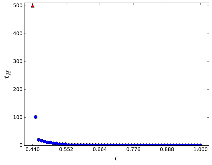
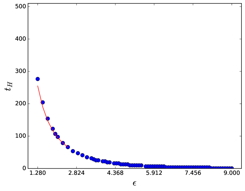
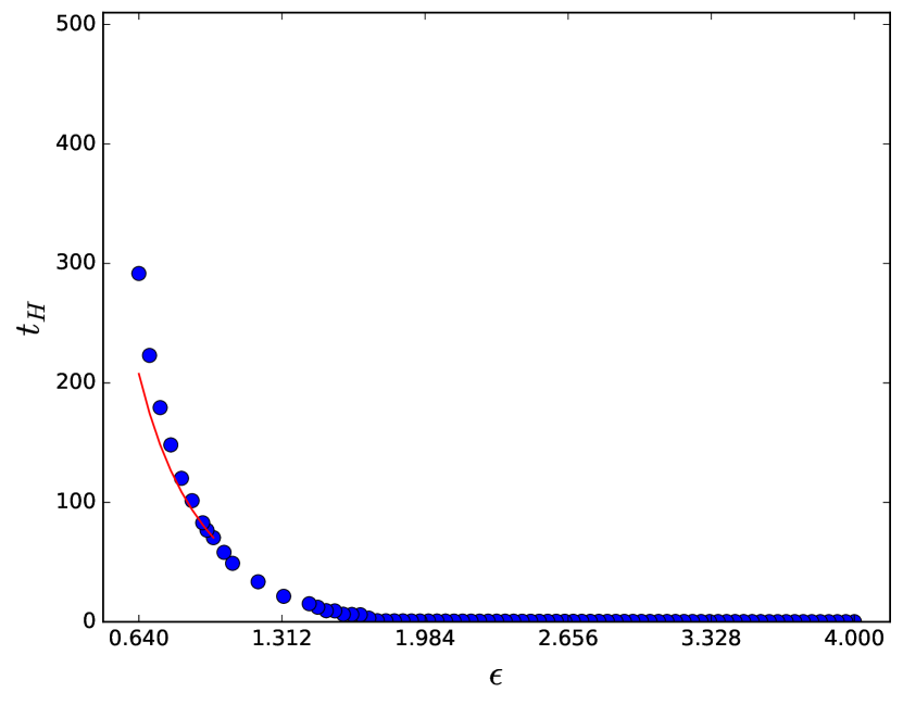
Based on the perturbative scaling relation, initial data can be divided into several classes with respect to behavior at low amplitudes, as illustrated in figure 1 for massless scalars. Stable initial data evolve indefinitely without forming a horizon. In practice, we identify this type of behavior in numerical evolutions by noting rapid horizon formation at high amplitude with a vertical asymptote in $t_{H}$ just above some critical amplitude. In our numerical results, we see a sudden jump at the critical amplitude to evolutions with no horizon formation to a large time $t_{lim}$, possibly with a small window of amplitudes with large $t_{H}$ just above the critical amplitude. In a few cases, we have captured a greater portion of the asymptotic region. See figure 1(a). Unstable initial data, in contrast, forms a horizon at all amplitudes following the perturbative scaling relation $t_{H}\propto\epsilon^{-2}$ as $\epsilon\to 0$. In our analysis, we will verify this scaling by fitting $t_{H}$ to a power law as described in section II.2 below; if we limit the fit to smaller values of $\epsilon$, the scaling becomes more accurate. Figure 1(b) shows unstable data. The red curve is of the form $t_{H}=a\epsilon^{-2}+b$ with $a,b$ determined by matching the curve to the data for the largest two amplitudes with $t_{H}\geq 60$ (not a best fit); note that the data roughly follow this curve. The categorization of different initial data profiles with similar characteristic widths into stable and unstable is robust for massless and massive scalars Deppe and Frey (2015); small and large width initial data are unstable, while intermediate widths are stable. One of the major results of this paper is determining how the widths of initial data in these “islands of stability” vary with scalar mass.

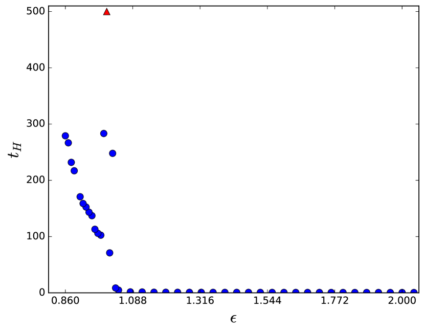
A priori, there are other possible types of behavior, at least beyond the first subleading order in perturbation theory, that is, at finite $\epsilon$. Metastable initial data collapse with $t_{H}\propto\epsilon^{-p}$ with $p>2$ at small but not arbitrarily small amplitudes (or another more rapid growth of $t_{H}$ with decreasing amplitude). We will find this type of behavior common on the “shoreline” of islands of stability where stable behavior transitions to unstable. As we will discuss further below, metastable behavior may or may not continue as $\epsilon\to 0$; in principle, as higher order terms in perturbation theory become less important, the behavior may shift to either stable or unstable as described above. In principle, initial data that are stable at third order in perturbation theory but unstable at higher order could have metastable scaling even in the $\epsilon\to 0$ limit, though our numerical study cannot address this case. We in fact find circumstantial evidence in favor of the different possibilities. In the case that the $\epsilon\to 0$ behavior is perturbatively unstable, the perturbative scaling $t_{H}\propto\epsilon^{-2}$ only appears for larger $t_{H}$ than the typical unstable case; it may therefore be reasonable for the reader to consider metastable initial data as part of a second order transition between unstable and stable classes of initial data. Figure 1(c) shows metastable initial data that continue to collapse to times $t_{H}\sim 0.6t_{lim}$ but more slowly than $\epsilon^{-2}$; note that $t_{H}$ for collapsed evolutions at small amplitudes lies significantly above the curve $t_{H}=a\epsilon^{-2}+b$ (which is determined as in figure 1(b)). There was one additional type of behavior identified by Deppe and Frey (2015), which was called “quasi-stable” initial data at the time since the low-amplitude behavior was not yet clear. We find here that these initial data are typically stable at small amplitude but exhibit irregular behavior in $t_{H}$ as a function of $\epsilon$, so we will denote them as irregular initial data; irregular behavior may be strongly non-monotonic or even exhibit some evidence of chaos. Figure 1(d) shows an example of irregular initial data. Later, we will see more striking examples of this behavior for massive scalars.

We emphasize that we are not claiming that metastable or irregular behavior persist to arbitrarily small amplitudes (though a priori metastable behavior could). In that sense, the multiscale perturbation theory suggests that the only two classes of stability behavior are stable and unstable with $t_{H}\propto\epsilon^{-2}$ scaling as $\epsilon\to 0$. However, it is also important to understand physics outside the perturbative regime, and classifying the behavior of AdS when higher-order or nonperturbative effects contribute is still of interest. For example, it is clear that metastable initial data (as defined precisely below) do not exhibit perturbatively unstable behavior for $t_{H}$ values as small as other unstable initial data, even in the cases where it may at all. This may help understanding the breakdown of the multiscale perturbation theory. Similarly, irregular initial data lead to qualitatively different behavior even visually and suggests that nonperturbative dynamics are important. It is in the spirit of looking beyond the multiscale perturbation theory that we call metastable and irregular initial data independent classes of behavior, even if they are not quite on the same standing as perturbatively stable or unstable classes. This paper presents the first systematic mapping of where these distinct behaviors appear.

II.2 Methods

For spherically symmetric motion, the Klein-Gordon equation for scalar mass $\mu$ can be written in first order form as

$$\phi_{,t}= Ae^{-\delta}\Pi,\quad\Phi_{,t}=\left(Ae^{-\delta}\Pi\right)_{,x},$$ (2)

$$\Pi_{,t}= \frac{(Ae^{-\delta}\tan^{d-1}(x)\Phi)_{,x}}{\tan^{d-1}(x)}-\frac{e^{-\delta}\mu^{2}\phi}{\cos^{2}(x)}\ ,$$ (3)

where $\Pi$ is the canonical momentum and $\Phi=\phi_{,x}$ is an auxiliary variable. The Einstein equation reduces to constraints, which can be written as

$$\delta_{,x}= -\sin(x)\cos(x)(\Pi^{2}+\Phi^{2})$$ (4)

$$M_{,x}= \left(\tan(x)\right)^{d-1}\left[A\frac{\left(\Pi^{2}+\Phi^{2}\right)}{2}+\frac{\mu^{2}\phi^{2}}{2\cos^{2}(x)}\right],$$ (5)

$$A= 1-2\frac{\sin^{2}(x)}{(d-1)}\frac{M}{\tan^{d}(x)},$$ (6)

where the mass function $M$ asymptotes to the conserved ADM mass at the boundary $x=\pi/2$. We will restrict to $d=4$ spatial dimensions. Since results are robust against changes in the type of initial data Deppe and Frey (2015), we can take the initial data to be a Gaussian of the areal radius in the canonical momentum and trivial in the field. Specifically,

$$\Pi(t=0,x)=\epsilon\exp\left(-\frac{\tan^{2}(x)}{\sigma^{2}}\right),\quad\phi(t=0,x)=0.$$ (7)

The width $\sigma$ and field mass $\mu$ constitute the parameter space for our stability phase diagram.

We solve the Klein-Gordon evolution equations (2,3) and Einstein constraint equations (4,5) numerically using methods similar to those of Maliborski and Rostworowski (2013b) on a spatial grid of $2^{n}+1$ grid points; we discuss the convergence properties of our code in the appendix. We denote the approximate horizon position $x_{H}$ and formation time $t_{H}$ by the first point such that $A(x_{H},t_{H})\leq 2^{7-n}$. In detail, we evolve the system in time using a 4th-order Runge-Kutta stepper and initially use a 4th-order Runge-Kutta spatial integrator at resolution $n=14$. If necessary, we switch to a 5th-order Dormand-Prince spatial integrator and increase resolution near horizon formation. Due to time constraints, we do not increase the resolution beyond $n=21$ for any particular calculation; if a higher resolution would be required to track horizon formation for a given amplitude, we exclude that amplitude.

To determine the stability class of initial data with a given width $\sigma$, we allow evolutions to run to a maximum time of $t_{lim}=500$ in AdS units, so $t_{lim}$ is a lower limit for $t_{H}$ for amplitudes that do not form a horizon within that time. Normally, however, if the initial data appear unstable, we only evolve amplitudes with $t_{H}\lesssim 0.6t_{lim}$; this is partly to save computational resources and partly to distinguish stable evolutions from collapsing ones. For unstable or metastable initial data, we find the best fit of the form $t_{H}=a\epsilon^{-p}+b$ to evolutions with $t_{H}>t_{fit}$, where $t_{fit}$ is a constant time chosen such that amplitudes with evolutions that last longer are usually roughly perturbative; in practice, $t_{fit}=60$ gives results close to the perturbative result $p=2$ for evolutions expected to be unstable from the literature, but we will also consider $t_{fit}=80,100$ as described below. In other words, since a given amplitude $\epsilon$ may be in the perturbative scaling regime for one set of initial data but nonperturbative for another, we compare initial data at similar horizon formation times (addressing the onset of perturbative behavior). Choosing $t_{fit}$ as above gives consistent values of the fit parameters for the three values of $t_{fit}$ for the largest and smallest initial data widths, which are unstable.

III Phase Diagram of Stability

Here we give our main result, the phase diagram of stability classes as a function of initial profile width and scalar mass, along with a more detailed discussion of the scaling of horizon formation time with amplitude for varying initial data.

Figure 2: Stability phase diagram as a function of initial data width $\sigma$ and scalar mass $\mu$. Blue diamonds represent stable initial data, orange circles unstable initial data, green triangles metastability, and red squares irregular behavior.

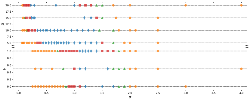
The stability phase diagram for spherically symmetric scalar field collapse in AdS₅, treating the width $\sigma$ of initial data and scalar field mass $\mu$ as tunable parameters, appears in figure 2. Each $(\mu,\sigma)$ combination that we evolved numerically is indicated by a point, with blue diamonds and orange circles representing stable and unstable initial data respectively. The metastable class is represented by green triangles, while the irregular class is represented by red squares. Note that the graph has been divided into two regions with different scales, separated by a break: $0\leq\mu\leq 1$ is pictured on the bottom, while $5\leq\mu\leq 20$ is pictured on the top. At a glance, two features of the stability phase diagram are apparent: as $\mu$ increases, the island of stability moves toward smaller values of $\sigma$ and takes up a gradually larger range of $\sigma$. To be specific, the stable class of initial data is centered at $\sigma=\bar{\sigma}\sim 1.4$ and has a width of $\Delta\sigma\sim 0.7$ for $\mu=0,0.5$, with $\bar{\sigma}\sim 1.2$ for $\mu=1$. $\Delta\sigma$ increases to $\sim 1.1$, and the island of stability is centered at $\bar{\sigma}\sim 0.9$ for $\mu=5,10$, while $\Delta\sigma\sim 1.2$ for $\mu=15,20$ with the stable class centered at $\bar{\sigma}\sim 0.8$. Note that the transition between “light field” and “heavy field” behavior occurs for $\mu>1$ in AdS units.

The metastable and irregular classes appear at the shorelines of the island of stability, the boundary between unstable and stable classes. In particular, the slope of the power law $t_{H}\sim\epsilon^{-p}$ as $\epsilon\to 0$ increases as the width moves toward the island of stability, leading to metastable behavior. We find metastability at the large $\sigma$ shoreline for all $\mu$ values considered and also at the small $\sigma$ shoreline for several scalar masses. It seems likely that metastable behavior appears in only a narrow range of $\sigma$ for larger $\mu$, which makes it harder to detect in a numerical search, leading to its absence in some parts of the stability phase diagram. We find irregular behavior at the small $\sigma$ shoreline for every mass and at the large $\sigma$ boundary for large $\mu$, closer to stable values of $\sigma$ than metastable initial data. This class of initial data includes a variety of irregular and non-monotonic behavior, as detailed below. Evidence for chaotic behavior especially becomes more prominent at larger values of $\mu$, as we will discuss below.

III.1 Metastable versus unstable initial data

While stable and irregular initial data are typically apparent by eye in a plot of $t_{H}$ vs $\epsilon$, distinguishing the unstable from metastable classes is a quantitative task. As we described in section II.2, we find the least squares fit of $t_{H}=a\epsilon^{-p}+b$ to all evolutions with $t_{H}>t_{fit}$ for the given $(\mu,\sigma)$, running over values $t_{fit}=60,80,100$. Using the covariance matrix of the fit, we also find the standard error for each fit parameter. We classify a width as having unstable evolution if the best fit value of $p$ is within two standard errors of $p=2$ for $t_{fit}=60,80$ or one standard error for $t_{fit}=100$ (due to a smaller number of data points, the standard errors for $t_{fit}=100$ tend to be considerably larger). In contrast, we classify a width as having metastable evolution if the best fit $p$ is statistically significantly different from $2$ (in that the best fit value is more than 2 standard errors from $p=2$ for $t_{fit}=60,80$ and more than 1 standard error from $p=2$ for $t_{fit}=100$). This indicates that either further subleading contributions in a perturbative expansion of $t_{H}$ are non-negligible in this regime for metastable initial data or that possibly metastable initial data are stable at the first nontrivial order in perturbation theory. Considering larger values of $t_{fit}$ helps to ensure that the leading perturbative terms do not come to dominate for particular initial profile at the smallest computationally accessible amplitude values. In the case that the fit to $t_{H}=a\epsilon^{-p}+b$ has large reduced $\chi^{2}$ or is sensitive to fitting algorithm, the data are not well-described by our fitting function, so we classify it as irregular (see the next subsection).

Figure 3: Coefficient $a$ from the fit $t_{H}=a\epsilon^{-p}+b$ as a function of width $\sigma$ using $t_{fit}=60$. Shows data for $\mu=0$ (green diamonds), $0.5$ (red triangles), $1$ (yellow stars), 5 (black circles), 10 (cyan squares), 15 (magenta Y), and 20 (blue circles). The orange line is the best power law fit.

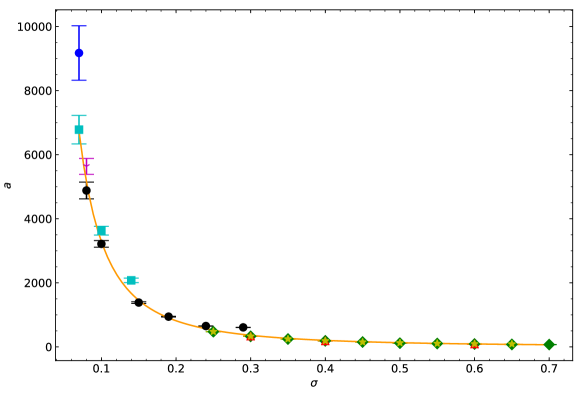
The fits $t_{H}=a\epsilon^{-p}+b$ allow us to explore the time scale of horizon formation across the stability phase diagram, for example through a contour plot of one of the coefficients vs $\sigma$ and $\mu$. In most cases, this has not been informative, but an intriguing feature emerges if we plot the normalization coefficient $a$ vs $\sigma$ for unstable initial data at small $\sigma$, as shown in figure 3 for $t_{fit}=60$. By eye, the coefficient is reasonably well described by the fit $a=(32.0\pm 0.3)\sigma^{-(2.01\pm 0.02)}$ (values following $\pm$ are standard errors of the best fit values) independent of scalar field mass. This is not born out very well quantitatively; the reduced $\chi^{2}$ for the fit is $\chi^{2}$/degrees of freedom (d.o.f.)$=180$, indicating a poor fit. However, the large $\chi^{2}$ seems largely driven by a few outlier points with large scalar mass, so it is tempting to speculate that the gravitational collapse in this region of parameter space is driven by gradient energy, making all fields effectively massless at narrow enough initial $\sigma$. The picture is qualitatively similar if we consider the parameter $a$ for $t_{fit}=80,100$ instead.

(a) $\mu=15,\sigma=1.5$

(b) $\mu=5,\sigma=1.7$

(c) $\mu=0,\sigma=1.8$

(d) $\mu=0.5,\sigma=1.7$

Figure 4: Metastable behavior: blue dots represent horizon formation and red triangles a lower limit on $t_{H}$. Magenta curves are fits $t_{H}=a\epsilon^{-p}+b$ over the shown range of amplitudes. Insets show the fit region with log-log scale; note that the fit is not strictly a power law, so the fits are not straight lines. See table 1 for best fit parameters. Red lines in insets are $\epsilon^{-2}$ power laws normalized to the $t_{H}$ of the smallest amplitude shown.

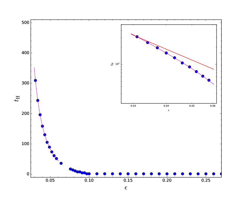
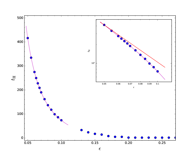
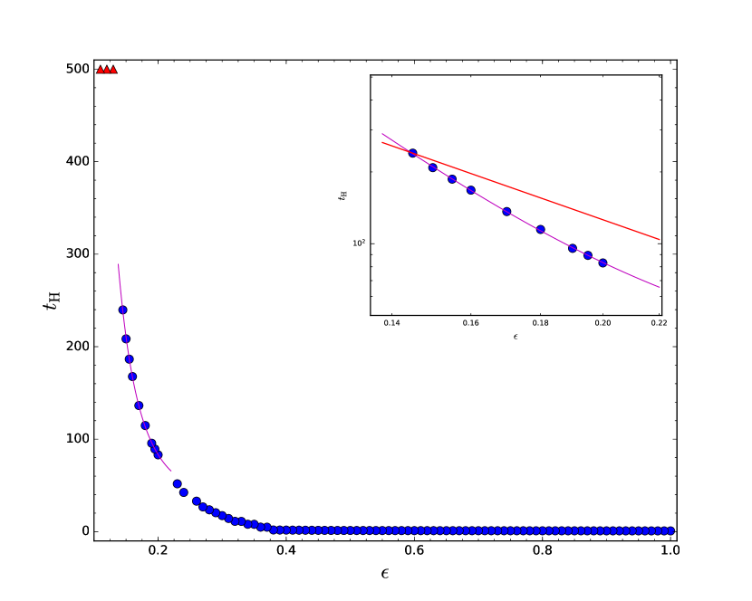
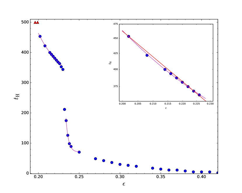
Several examples of metastable behavior appear in figure 4. These figures show both data from the numerical evolutions (blue dots and red triangles) and fits of the form $t_{H}=a\epsilon^{-p}+b$ for points with $t_{H}>t_{fit}=60$ (magenta curves). The best fit parameters are given in table 1 along with the standard errors (listed following $\pm$ for the fit values) and $\chi^{2}$ values. The insets show the fit region with a log-log scale and an additional line (red) showing an $\epsilon^{-2}$ power law normalized to fit the smallest amplitude shown in the inset. It is visually clear that $t_{H}$ grows faster than $\epsilon^{-2}$ for all these examples as $\epsilon$ decreases in the fit region (there is a significant constant offset in figure 4(d)).

Figures 4(a),4(b) demonstrate behavior typical of most of the instances of metastable initial data we have found; specifically, the initial data continue to collapse through horizon formation times of $t_{H}\sim 0.6t_{lim}$ but with $p$ significantly greater than the perturbative value of $p=2$. Note that the evolutions of figure 4(b) have been extended to larger values of $t_{H}$ to demonstrate that the evolutions continue to collapse to somewhat smaller amplitude values. Figure 4(b) is also of interest because its best fit value $p\approx 2.07\pm 0.02$ is approximately as close to the perturbative value as several stable sets of initial data but has a smaller standard error for the fit, so the difference from the perturbative value is more significant (again, the value following the $\pm$ is the standard error).

	$a$	$p$	$b$	$\chi^{2}/$d.o.f.
$\mu=15,\sigma=1.5$	$0.10\pm 0.01$	$2.33\pm 0.05$	$-27\pm 4$	0.7736
$\mu=5,\sigma=1.7$	$0.91\pm 0.06$	$2.07\pm 0.02$	$-33\pm 2$	0.5070
$\mu=0,\sigma=1.8$	$0.06\pm 0.02$	$4.3\pm 0.2$	$30\pm 5$	1.502
$\mu=0.5,\sigma=1.7$ ($t_{H}<0.4t_{lim}$)	$(4\pm 32)\times 10^{-45}$	$73\pm 5$	$70\pm 2$	5.409
($t_{H}>0.72t_{lim}$)	$0.02\pm 0.03$	$5.6\pm 0.8$	$260\pm 20$	1.078

Table 1: Best fit parameters for the cases shown in figure 4 restricting to $t_{H}>t_{fit}=60$ and as noted. Listed errors ($\pm$ values) are standard errors. $\chi^{2}/$d.o.f. is the reduced $\chi^{2}$ value used as a measure of goodness-of-fit.

Figure 4(c) shows metastable evolution to $t_{H}\lesssim 0.6t_{lim}$ but then a sudden jump to stability until $t=t_{lim}$. In the figure, the fit has been extended to the largest non-collapsing amplitude, which demonstrates that there is no collapse over a time period significantly longer than the fit predicts. This example argues that metastable data may in fact become stable at the smallest amplitudes. On the other hand, figure 4(d) shows a similar jump in $t_{H}$ to values $t_{H}<t_{lim}$; evolution at lower amplitudes shows metastable scaling with $p\approx 5.6\pm 0.8$ for $360<t_{H}<t_{lim}$. The figure also shows a metastable fit with larger reduced $\chi^{2}$ at larger amplitudes corresponding to $t_{fit}<t_{H}<0.4t_{lim}$. So this is another option: metastable behavior may transition abruptly to metastable behavior with different scaling (or possibly even perturbatively unstable behavior) at sufficiently small amplitudes. It is also reasonable to classify this case as irregular due to the sudden jump in $t_{H}$; we choose metastable due to the clean metastable behavior at low amplitudes.

Our point of view is that initial data in the metastable class are distinct from the unstable class at finite amplitudes corresponding to $t_{fit}<t_{H}<300$; they take longer to collapse at a fixed small value of $\epsilon$ than would be expected by the perturbative scaling. An alternate point of view is to ask whether we can determine if a given set of initial data is perturbatively unstable in the $\epsilon\to 0$ limit. We have already seen that metastable initial data do not follow the perturbative scaling when fit to $t_{H}=a\epsilon^{-p}+b$, the first two terms of the perturbative expansion. However, it is possible that a perturbative description applies but requires a further subleading term. To test this hypothesis, we fit unstable and metastable initial data to $t_{H}=a\epsilon^{-p}+b+c\epsilon^{2}$; as described earlier in this section, we determine if $p$ is within two standard errors of the perturbative value $p=2$ (or one standard error for $t_{fit}=100$).

The unstable class of initial data is instructive. For the new fits of unstable initial data, $p$ is statistically equal to 2, and the new values of $a,p,b$ are consistent with the values from the old fits to within two standard errors (or sometimes slightly more). The fit value of $c$ is uniformly within a standard error of zero, and, for the amplitude values in the fit region, the $\epsilon^{2}$ term is small compared to the constant and $\epsilon^{-2}$ terms. What is more, for some unstable initial data near the island of stability, the original $t_{H}=a\epsilon^{-p}+b$ fits for $t_{fit}=60$ have $p>2$ statistically; on the other hand, the new fits have $p=2$ within statistical error. In other words, the perturbative expansion is still valid but requires more terms. Part of the metastable class of initial data also behaves in this manner and could therefore be reasonably considered to be perturbatively unstable. Of the metastable initial data we found, these are $\sigma=1.9$ for $\mu=0$, $\sigma=0.8$ and 1.9 for $\mu=0.5$, $\sigma=0.7$ for $\mu=1$, $\sigma=1.7$ for $\mu=5$, $\sigma=0.155$ for $\mu=10$, $\sigma=0.11$ and 1.5 for $\mu=15$, and $\sigma=1.5$ for $\mu=20$. In addition, $\mu=1,\sigma=1.8$ and $\mu=10,\sigma=1.7$ initial data have similar behavior, but $p$ is not statistically consistent with 2 for any of the fit regions, though it is closer than in the original fits. On the other hand, the other metastable initial data ($\sigma=0.85$ and 1.8 for $\mu=0$, $\sigma=1.7$ and 1.8 for $\mu=0.5$, $\sigma=1.45$ for $\mu=10$, and $\sigma=1.4$ for $\mu=20$) show no evidence for perturbative behavior. Specifically, $p$ remains statistically larger than 2 for all fits, the $\epsilon^{2}$ term in the new fit is roughly the same magnitude as the other terms, and the $a,p,b$ values in the new fits are not statistically consistent with the original fits.

To check if perturbative scaling might be masked by numerical errors, we have also fit these remaining metastable data ($\sigma=0.85,1.8$ for $\mu=0$, $\sigma=1.8$ for $\mu=0.5$, $\sigma=1.8$ for $\mu=1$, $\sigma=1.45,1.7$ for $\mu=10$, and $\sigma=1.4$ for $\mu=20$) with $t_{H}=a\epsilon^{-p}+b\epsilon^{-1}+c$. Of these, only the $\mu=1,\sigma=1.8$ and $\mu=10,\sigma=1.7$ initial data have best fit $p$ values statistically consistent with $p=2$. However, except for $\mu=1,\sigma=1.8$ initial data, the best fit $p$ values are all further from $p=2$ in absolute terms (usually substantially); the main effect of including the $\epsilon^{-1}$ term is to increase the standard error on the best fit for $p$. Therefore, it is not clear that potential numerical errors alone can be responsible for the observed deviation from perturbative scaling. We would also point out that, even if the extra $\epsilon^{-1}$ term turns out to be important for these initial data, the fact that it is only important at the boundary of the island of stability indicates a change in behavior for these mass/width combinations as compared to those farther from the stable region. This justifies a separate classification related to the slower entry of these mass/width combinations into the perturbative regime (as measured by horizon formation time).

III.2 Irregular behaviors

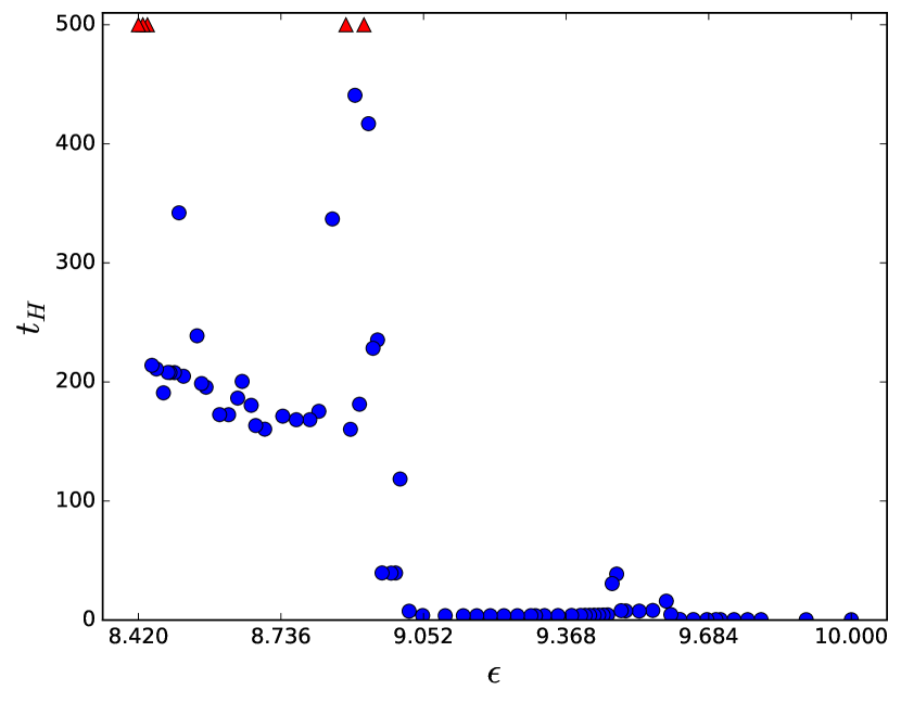
We have found a variety of irregular behaviors at the transition between the metastable and stable classes which we have classified together as irregular initial data; however, it may be better to describe them as separate classes. The stability phase diagram 2 indicates that the irregular class extends along the “inland” side of the small $\sigma$ shoreline and at least part of the large $\sigma$ shoreline of the island of stability. What is not clear from our evolutions up to now is whether each type of behavior appears along the entire shoreline or if they appear in pockets at different scalar field masses. Examples of each type of behavior that we have found appear in figure 5.

(a) $\mu=0.5,\sigma=1$

(b) $\mu=5,\sigma=0.34$

(c) $\mu=20,\sigma=0.16$

(d) $\mu=20,\sigma=0.19$

Figure 5: Irregular behavior: blue dots represent horizon formation and red triangles a lower limit on $t_{H}$.

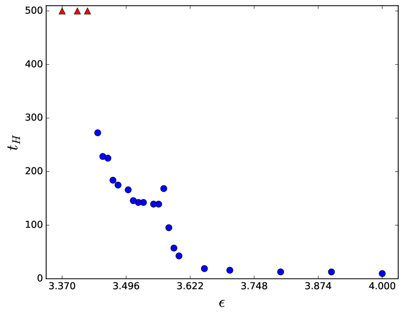
The first type of irregular behavior, shown in figure 5(a), is monotonic ($t_{H}$ increases with decreasing $\epsilon$ as usual), but it is not well fit by a power law. In fact, this behavior would classify as metastable by the criterion of section III.1 in that the power law of the best fit $t_{H}=a\epsilon^{-p}+b$ is significantly different from $p=2$, except for the fact that the reduced $\chi^{2}$ value for the fit is very large (greater than 10) and also that different fitting algorithms can return significantly different fits, even though the data may appear to the eye like a smooth power law. In any case, this type of behavior apparently indicates a breakdown of metastable behavior and hints at the appearance of non-monotonicity. So far, our evolutions have not demonstrated sudden jumps in $t_{H}$ typical of stability at low amplitudes, however.

Figure 5(b) exemplifies non-monotonic behavior in the irregular class. This type of behavior, which was noted already by Buchel et al. (2013), involves one or more sudden jumps in $t_{H}$ as $\epsilon$ decreases, which may be followed by a sudden decrease in $t_{H}$ and then resumed smooth monotonic increase in $t_{H}$. There are suggestions that this type of initial data is stable at low amplitudes due to the usual appearance of non-collapsing evolutions, but it is worth noting that these amplitudes could instead experience another jump and decrease in $t_{H}$, just at $t_{H}>t_{lim}$. Finally, Deppe and Frey (2015) studied this type of behavior in some detail, denoting it as “quasi-stable.”

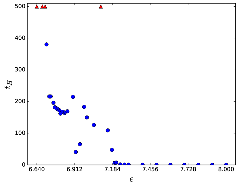
Some irregular initial data demonstrate evidence of chaotic behavior, in that $t_{H}$ appears to be sensitive to initial conditions (ie, value of amplitude) over some range of amplitudes. This type of behavior appears over the range of masses (see figure 1(d) for a mild case for massless scalars), but it is more common and more dramatic at larger $\mu$. Figures 5(c),5(d) represent the most extreme behavior of this type among the initial data that we studied with collapse at $t_{H}<50$ not very far separated from amplitudes that do not collapse for $t<t_{lim}$ along with an unpredictable pattern of variation in $t_{H}$. This type of evidence for chaotic behavior has been seen previously in the collapse of transparent but gravitationally interacting thin shells in AdS Brito et al. (2016) as well as in the collapse of massless scalars in AdS₅ Einstein-Gauss-Bonnet gravity Deppe et al. (2015, 2016); these references speculated that the $t_{H}$ vs $\epsilon$ curve is fractal. In both cases, this type of behavior is hypothesized to be due to the transfer of energy between two infalling shells, with horizon formation only proceeding when one shell is sufficiently energetic. In the latter case, the extra scale of the theory (given by the coefficient of the Gauss-Bonnet term in the action) leads the single initial pulse of scalar matter to break into two pulses.

We should therefore ask two questions: does this irregular behavior show evidence of true chaos, and is a similar mechanism at work here? We note first that Deppe et al. (2016) found evidence (using a modified box test) that the $t_{H}$ vs $\epsilon$ curve has a non-integer fractal dimension for plots visually similar to our figures 5(c),5(d). Here, to quantify the presence of chaos, we examine the difference in time evolution between similar initial conditions (nearby amplitudes), which diverge exponentially in chaotic systems. Specifically, any quantity $\Delta$ should satisfy $|\Delta|\propto\exp(\lambda t)$ for Lyapunov coefficient $\lambda$. Our characteristic will be the upper envelope of the Ricci scalar at the origin per light crossing time, $\bar{\mathcal{R}}(t)$. We consider three sets of irregular initial data: a massless scalar of width $\sigma=1.1$ with amplitudes $\epsilon=1.02,1.01,1.00$ (see figure 1(d)), a $\mu=5$ massive scalar of width $\sigma=0.34$ and $\epsilon=3.52,3.51,3.50$, and a $\mu=20$ scalar of width $\sigma=0.19$ and $\epsilon=6.98,6.95,6.92$ (figure 5(d)). We also determined the Lyapunov coefficient for unstable initial data with $\mu=0.5$, $\sigma=0.3$, and $\epsilon=1.22,1.20,1.18$ for comparison.

(a) Upper envelope of Ricci scalar at origin

(b) $\log|\Delta|$ vs. $t_{mid}$

Figure 6: Left: The upper envelope of the Ricci scalar for amplitudes $\epsilon_{1}=3.50$ (blue circles), $\epsilon_{2}=3.51$ (red triangles), and $\epsilon_{3}=3.52$ (green squares) for $\mu=5,\sigma=0.34$. Right: $\log(|\Delta_{12}|)$ and best fit (blue circles and line) and $\log(|\Delta_{23}|)$ and best fit (red squares and line), calculated as a function of the midpoint $t_{mid}$ of the time interval.

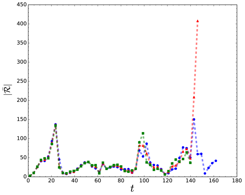
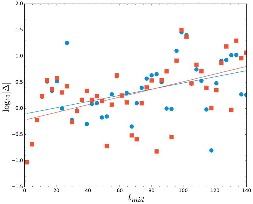
Figure 6 details evidence for chaotic evolution in the $\mu=5,\sigma=0.34$ case; figure 6(a) shows our characteristic function $\bar{\mathcal{R}}(t)$ for the amplitudes $\epsilon_{1}=3.50$, $\epsilon_{2}=3.51$, and $\epsilon_{3}=3.52$. By eye, $\bar{\mathcal{R}}$ shows noticeable differences after a long period of evolution. These are more apparent in figure 6(b), which shows the log of the differences $\Delta_{ab}\equiv\bar{\mathcal{R}}_{\epsilon_{a}}-\bar{\mathcal{R}}_{\epsilon_{b}}$, along with the best fits. Although there is considerable noise — or oscillation around exponential growth — in the differences (leading to $R^{2}$ values $\sim 0.2,0.26$ for the fits), the average slope gives Lyapunov coefficient $\lambda=0.007$ (within the error bar of each slope), and each slope differs from zero by more than 3 standard errors. One interesting point is that the $t_{H}$ vs $\epsilon$ curve in figure 5(b) does not appear chaotic to the eye, even though it shows some of the mathematical signatures of chaos at least for $\epsilon_{1}<\epsilon<\epsilon_{3}$ (the visible spike in $t_{H}$ is at $\epsilon\sim 3.57$).

The story is similar for the massless and $\mu=20$ cases we studied, which exhibit $\lambda$ values that differ from zero by at least 1.9 standard errors; see table 2. This is a milder version of the behavior noted by Brito et al. (2016); Deppe et al. (2015, 2016), especially for the $\mu=5$ case studied. One thing to note is that the strength of oscillation in $\log(|\Delta|)$ around the linear fit increases with increasing mass, so that the two best fit Lyapunov exponents for $\mu=20$ are no longer consistent with each other at the 1-standard deviation level. We should note, however that the unstable initial data with $\mu=0.5,\sigma=0.3$ also exhibits a statistically positive Lyapunov exponent, though we should note that the value of $\lambda$ quoted in table 2 includes the time shortly before horizon formation, which does increase $\lambda$ somewhat (though not more than the quoted error).

		$\lambda$	average $\lambda$
$\mu=0,\sigma=1.1$	$\Delta_{12}$	$0.011\pm 0.005$	0.011
	$\Delta_{23}$	$0.011\pm 0.005$
$\mu=0.5,\sigma=0.3$	$\Delta_{12}$	$0.021\pm 0.0007$	0.022
	$\Delta_{23}$	$0.024\pm 0.001$
$\mu=5,\sigma=0.34$	$\Delta_{12}$	$0.006\pm 0.002$	0.007
	$\Delta_{23}$	$0.007\pm 0.002$
$\mu=20,\sigma=0.19$	$\Delta_{12}$	$0.046\pm 0.009$	0.032
	$\Delta_{23}$	$0.019\pm 0.007$

Table 2: Best fit Lyapunov coefficients $\lambda$ for adjacent amplitude pairs and average $\lambda$ value for each $\mu,\sigma$ system studied. Standard errors are given following $\pm$ signs.

(a) $\mu=5,\sigma=0.34,\epsilon=3.51$

(b) $\mu=0.5,\sigma=0.3,\epsilon=1.20$

Figure 7: Trajectories in $\Pi(x=0),\phi(x=0)$ phase space for one irregular and one unstable evolution. Trajectories are shown for $t<50$.

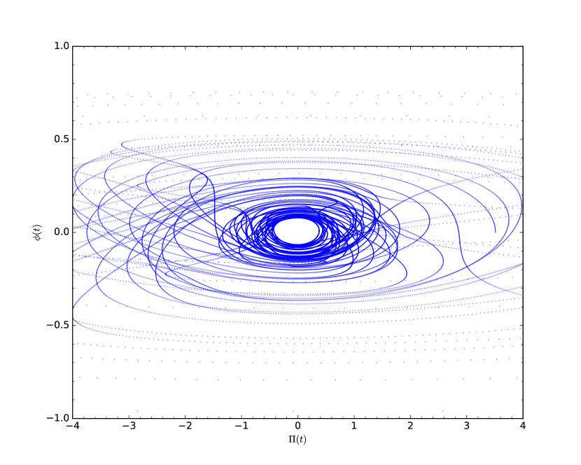
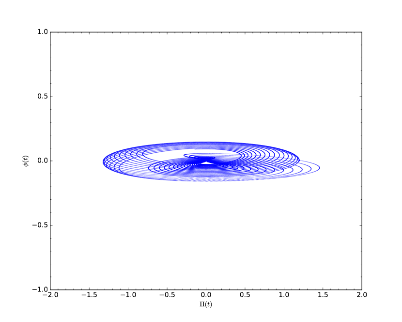
Since the Lyapunov coefficients do not distinguish the irregular and unstable cases, we also consider the phase space trajectories of the evolutions. Following de Oliveira et al. (2012), we consider the trajectory of evolutions in $\Pi$ and $\phi$ evaluated at the origin for $t\leq 50$ in figure 7. Neither the $\mu=5,\sigma=0.34,\epsilon=3.51$ (figure 7(a)) or $\mu=0.5,\sigma=0.3,\epsilon=1.20$ (figure 7(b)) trajectories close, though there is a clear difference. Specifically, the former trajectory is visually disorganized (that is, strongly varying orbits) with very rapid motion (seen in the gap between points on the trajectory between plotted time steps). Meanwhile, the latter motion is comparatively regular, typical of quasi-periodic motion. Figure 7(a) is typical of turbulence and clearly shows that these evolutions are nonperturbative, even though $t_{H}$ is large (well into the perturbative regime for unstable initial data).

To sum up, we have identified irregular initial data that show evidence of chaotic behavior. Specifically, several of the $t_{H}$ vs $\epsilon$ curves appear qualitatively similar to analogous plots in Brito et al. (2016); Deppe et al. (2015, 2016), which were demonstrated to have fractal-like behavior (including fractional fractal dimension in one case). Furthermore, a number of cases of irregular initial data (and some unstable) have positive Lyapunov exponents; phase space trajectories for irregular initial data show very rapid motion typical of turbulence, while unstable initial data have more regular trajectories. Taken together, this is strong evidence for chaotic behavior for some irregular initial data, similar to that discussed in other studies of gravitational collapse in AdS. Furthermore, this is the first evidence of chaos in the $t_{H}$ vs $\epsilon$ curve for gravitational collapse of a massless scalar in AdS to our knowledge.

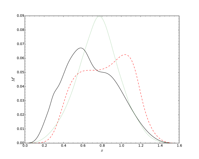
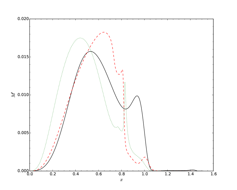
The mechanism underlying the possibly chaotic behavior seems somewhat different or at least weaker than the two-shell or Einstein-Gauss-Bonnet systems. When examining the time evolution of the mass distributions of these data, we see a single large pulse of mass energy that oscillates between the origin and boundary without developing a pronounced peak. However, there is also apparently a smaller wave that travels across the large pulse. We can see this by comparing snapshots of the mass distribution at different times, as in figure 8. In the massless case examined, this wave deforms the pulse, leading to a double-shoulder appearance seen at two times in figure 8(a). In the $\mu=5,\sigma=0.34$ case, the secondary wave is more like a ripple, usually smaller in amplitude but more sharply localized, as toward the right side of the main pulse in figure 8(b). So the chaotic behavior may be caused by the relative motion of the two waves, rather than energy transfer between two shells. In this hypothesis, a horizon would form when both waves reach the neighborhood of the origin at the same time.

(a) $\mu=0,\sigma=1.1,\epsilon=1.01$, at times $t=60$ (solid black), $t=62$ (dashed red), $t=64$ (dotted green)

(b) $\mu=5,\sigma=0.34,\epsilon=3.52$, at times $t=132$ (solid black), $t=137$ (dashed red), $t=140$ (dotted green)

Figure 8: Radial derivative of the mass function at the indicated time for two systems that show evidence of chaos. Note the appearance of a secondary wave on top of the main pulse. $(\mu,\sigma,\epsilon)$ as indicated.

As a note, we have run convergence tests on several sets of irregular initial data and find that our calculations are convergent overall, as expected (even at lower resolution than we used). In particular, the massless scalar evolutions studied in table 2 are convergent already at resolution given by $n=12$ (note that we typically start at $n=14$); we also observe convergent behavior for the $\mu=5$ evolutions discussed in table 2. We have therefore validated that nonmonotonic behavior and even evidence of chaos occurs. The only caveat may be for some of the apparently initial data with scalar mass $\mu=20$, which nonetheless appears well-behaved according to other indicators. The reader may or may not wish to take them at face value but should recall that we have presented other chaotic initial data with rigorously convergent evolutions. See the appendix for a more detailed discussion.

IV Spectral analysis

As we discussed in the introduction, instability toward horizon formation proceeds through a turbulent cascade of energy to shorter wavelengths or, more quantitatively, to 1st-order scalar eigenmodes with more nodes. Inverse cascades are typical of stable evolutions. Therefore, understanding the energy spectrum of our evolutions, both initially and over time, sheds light on the behavior of the self-gravitating scalar field in asymptotically AdS spacetime, providing a heuristic analytic understanding of the stability phase diagram.

The (normalizable) eigenmodes $e_{j}$ are given by Jacobi polynomials as

$$e_{j}(x)=\kappa_{j}\cos^{\lambda_{+}}(x)P^{(d/2-1,\sqrt{d^{2}+4\mu^{2}}/2)}_{j}(\cos(2x))$$ (8)

($\kappa_{j}$ is a normalization constant) with eigenfrequency $\omega_{j}=2j+\lambda_{+}$ and $\lambda_{+}=(d+\sqrt{d^{2}+4\mu^{2}})/2$ in AdS_d+1 for $j=0,1,\cdots$ (see Aharony et al. (2000); Nastase (2015) for reviews). Including gravitational backreaction, we define the energy spectrum

$$E_{j}\equiv\frac{1}{2}\left(\Pi_{j}{}^{2}-\phi_{j}\ddot{\phi}_{j}\right),$$ (9)

where

$$\Pi_{j} = \left(\sqrt{A}\Pi,e_{j}\right),\quad\phi_{j}=\left(\phi,e_{j}\right),$$

$$\ddot{\phi}_{j} = \left(\cot^{d-1}(x)\partial_{x}\left[\tan^{d-1}(x)A\Phi\right]-\mu^{2}\sec^{2}(x)\phi,e_{j}\right),$$ (10)

and the inner product is $(f,g)=\int_{0}^{\pi/2}dx\tan^{d-1}(x)fg$. The sum of $E_{j}$ over all modes is the conserved ADM mass.

IV.1 Dependence on mass

(a) Best fit gaussian energy spectra.

(b) Best fit gaussian and zeroth eigenmode.

Figure 9: Left: Spectra of the best fit Gaussians (7) to the $j=0$ eigenmode for masses $\mu=0$ (blue circles), 0.5 (yellow squares), 1 (empty orange circles), 5 (green diamonds), 10 (empty cyan squares), 15 (upward red triangles), and 20 (downward purple triangles). Right: an overlay of the best fit Gaussian and $e_{0}$ eigenmode for $\mu=0$ (solid blue is best fit, orange dashed is eigenmode) and $\mu=20$ (solid green, red short dashes).

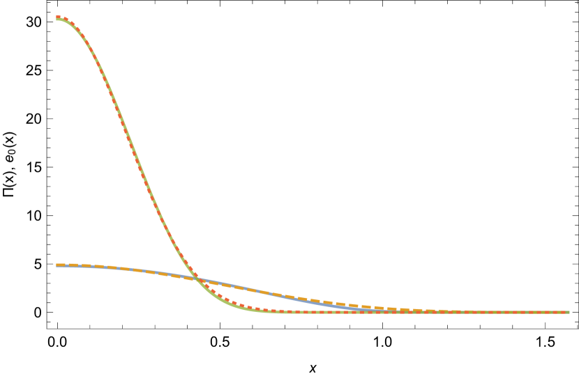
The most visibly apparent feature of the stability phase diagram of figure 2 is that the island of stability both expands and shifts to smaller widths as the scalar mass increases. As it turns out, the energy spectrum of the Gaussian initial data (7) provides a simple heuristic explanation.

It is well established both in perturbation theory and numerical studies that initial data given by a single scalar linear-order eigenmode is in fact nonlinearly stable, and the spectra of many quasi-periodic solutions are also dominated by a single eigenmode. As a result, we should expect Gaussian initial data that approximate a single eigenmode (which must be $j=0$ due to lack of nodes) to be stable. To explore how this depends on mass, we find the best fit values of $\epsilon,\sigma$ for the $j=0$ eigenmode for each mass that we consider (defined by the least-square error from the Gaussian to a discretized eigenmode); this is the “best approximation” Gaussian to the eigenmode. Then we find the energy spectrum of that best-fit Gaussian; these are shown in figure 9(a). From the figure, it is clear that the $j=0$ eigenmode is closer to a Gaussian at larger masses. That is, other eigenmodes contribute less to the Gaussian’s spectrum at higher masses (by several orders of magnitude over the range from $\mu=0$ to 20). Simply put, the shape of the $j=0$ eigenmode is closer to Gaussian at higher masses, which suggests that the island of stability should be larger at larger scalar field mass. Figure 9(b) compares the $j=0$ eigenmode and best fit Gaussian for $\mu=0$ and 20; on inspection, there is more deviation between the eigenmode and Gaussian for the massless scalar.

In addition, the best-fit Gaussian width decreases from $\sigma\sim 0.8$ for a massless scalar as the mass increases. At $\mu=20$, the best-fit width is $\sigma\sim 0.31$. This suggests that Gaussians that approximate the $j=0$ mode well enough are narrower in width at higher masses. An interesting point to note is that the island of stability for $\mu=0,0.5$ is actually centered at considerably larger widths than the best-fit Gaussian. This may not be surprising, since the best-fit Gaussians at low masses actually receive non-negligible contributions from higher mode numbers; moving away from the best-fit Gaussian can actually reduce the power in higher modes. For example, the stable initial data shown in figure 10(a) below have considerably less power in the $j=2$ mode.

IV.2 Spectra of different behaviors

(a) $\mu=0,\sigma=1.5$

(b) $\mu=0,\sigma=0.25$

(c) $\mu=5,\sigma=1.7$

(d) $\mu=0.5,\sigma=1$

(e) $\mu=5,\sigma=0.34$

(f) $\mu=20,\sigma=0.16$

Figure 10: Initial ($t=0$) energy spectra for the indicated evolutions. In order, these represent stable, unstable, metastable, monotonic irregular, non-monotonic irregular, and chaotic irregular initial data.

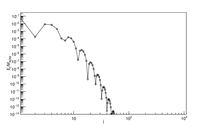
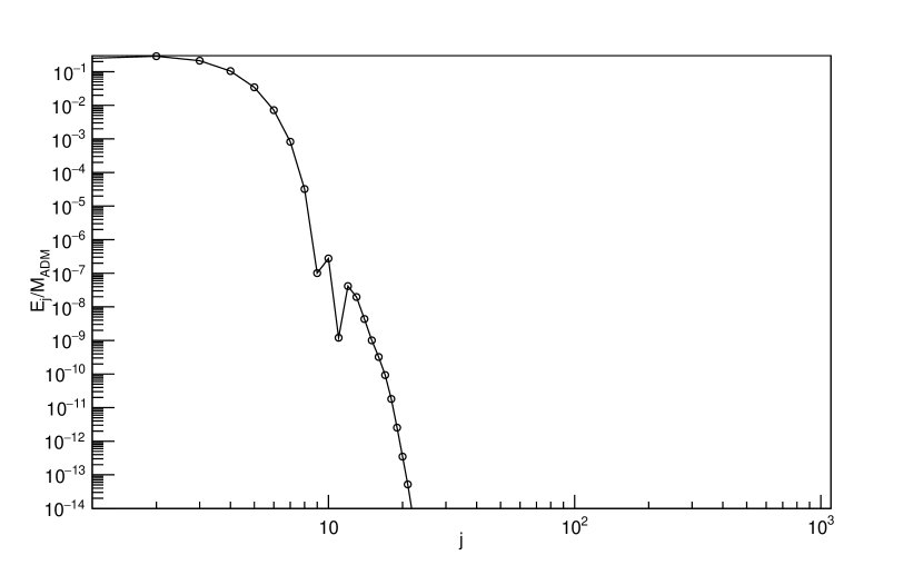
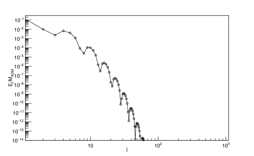
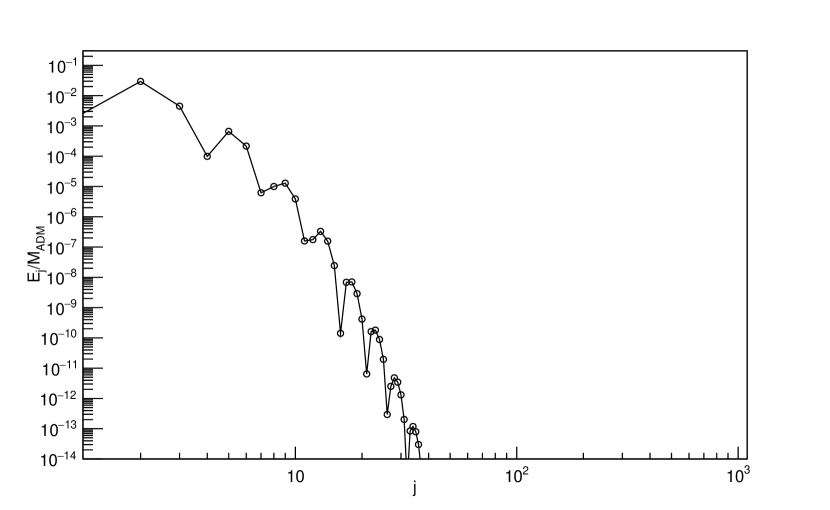
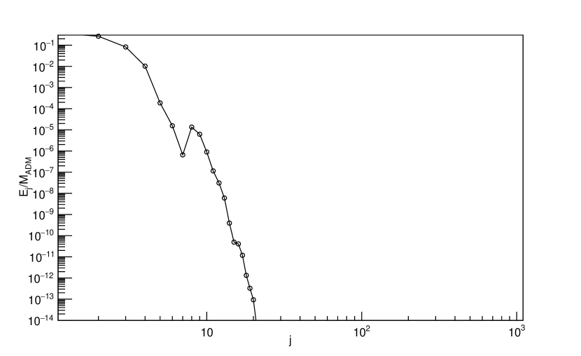
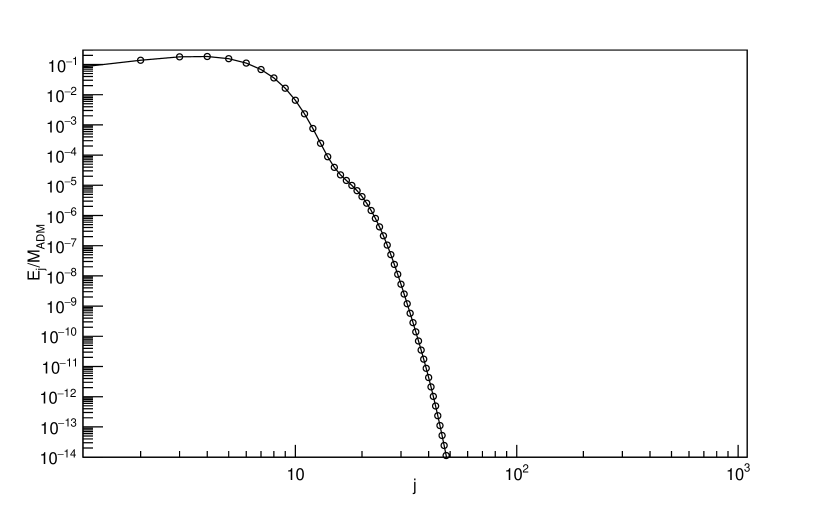
A key question that one might hope to answer is whether the stability class of a given $(\mu,\sigma)$ can be determined easily by direct inspection of the initial data without requiring many evolutions at varying amplitudes. The initial energy spectra for examples of each class, including monotonic, non-monotonic, and apparently chaotic irregular behaviors, are shown in figure 10. These spectra are taken from among the smallest amplitudes we evolved in order to minimize backreaction effects.

Unfortunately, the initial energy spectra do not seem to provide such a method for determining the stability class. Very broadly speaking, stable and metastable $(\mu,\sigma)$ correspond to initial spectra that drop off fairly quickly from the $j=0$ mode as $j$ increases, while unstable and irregular behaviors tend to have roughly constant or even slightly increasing spectra up to $j=5$ or $10$. However, figure 10(d) shows that some irregular initial data have spectra that decrease rapidly after a small increase from $j=1$ to $j=2$. Kinks in the spectrum are more prevalent for widths of the AdS scale or larger, while spectra for smaller widths tend to be smoother.

IV.3 Evolution of spectra

(a) $\mu=0,\sigma=1.8,\epsilon=0.13$

(b) $\mu=0,\sigma=0.25,\epsilon=2.28$

(c) $\mu=0.5,\sigma=1.7,\epsilon=0.216$

(d) $\mu=20,\sigma=0.19,\epsilon=6.95$

Figure 11: The time dependence of the energy spectra as a fraction of the total ADM mass for the indicated $\mu,\sigma,\epsilon$. Lower panels show the lowest 7 modes (in colors cyan, red, purple, green, yellow, brown, and gray respectively). Upper panels show cumulative energy to mode $j=0,1,2,4,8,16,32$ (in colors blue, orange, brown, yellow, aqua, red, and magenta).

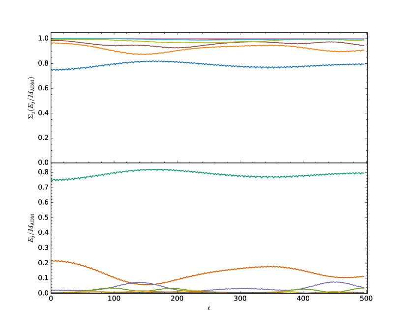
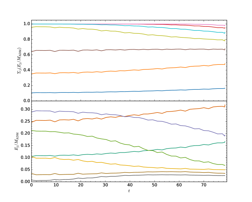
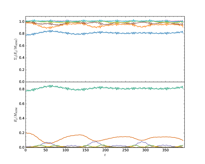
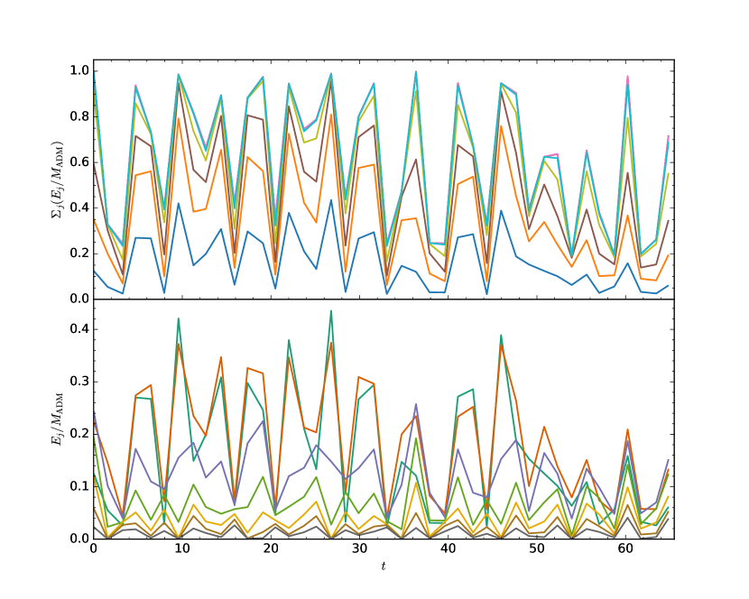
While the initial spectrum for a given $(\mu,\sigma)$ pair does not have predictive value regarding the future behavior as far as we can tell, the time dependence of the spectrum throughout the evolution of the system is informative. Figure 11 shows the time-dependence of spectra for examples of the stable, unstable, metastable, and chaotic irregular classes. In each figure, the lower panel shows the fraction $E_{j}/M_{ADM}$ in each mode up to $j=6$, while the upper panel shows the cumulative fraction $\sum_{j}E_{j}/M_{ADM}$ to the mode $2^{k}$ with $k=0$ to 5.

The difference between stable evolution in figure 11(a) and unstable evolution in figure 11(b) is readily apparent. As the evolution proceeds, we expect a cascade of energy into higher mode numbers, but inverse cascades to lower modes can also occur. The stable evolution shows a slow pattern of cascades and inverse cascades, in fact. On the other hand, the unstable evolution shows a nearly monotonic cascade of energy into the highest modes along with a simultaneous cascade of energy into the lowest modes (therefore depleting intermediate modes). These are common observations in the literature and are included here for completeness.

The metastable evolution shown in figure 11(c) is interesting in light of the stable and unstable spectra. The amplitude shown is from the unstable portion of figure 4(d), the part consistent with the perturbative scaling $t_{H}\sim\epsilon^{-2}$. However, the spectrum shows a similar pattern of slow cascades and inverse cascades to the stable initial data example, though on a somewhat faster time scale in this case. While perhaps surprising, this is in keeping with the similarities noted between the initial spectra in figures 10(a) and 10(c). We have also checked that the time-dependent spectrum at a higher amplitude with $t_{H}\sim 100$ follows the same pattern as 11(c); in fact, it looks essentially the same but simply ends at an earlier time. This lends some credence to the idea that metastable initial data are stable at lowest nontrivial order in perturbation theory, with instability triggered by higher-order corrections. Alternately, the instability could be caused by an oscillatory singularity in the perturbative theory, as discussed in Bizoń et al. (2015); Craps et al. (2015b); Deppe (2019); Dimitrakopoulos et al. (2016) in the case of two-mode initial data. These divergences do not appear in the energy spectrum.

Figure 11(d) shows the time-dependence of the spectrum in an irregular evolution, specifically $\mu=20,\sigma=0.19$ at $\epsilon=6.95$, which is in the chaotic region of the $t_{H}$ vs $\epsilon$ plot in figure 5(d). There is rapid energy transfer among modes, including cascades out of and inverse cascades into mode numbers $j\leq 32$ over approximately a light-crossing time. It is easy to imagine that horizon formation might occur at any of the cascades of energy into higher modes, leading to seemingly random jumps in $t_{H}$ as a function of amplitude.

(a) $\epsilon=1.01$

(b) $\epsilon=1.02$

Figure 12: Spectra at time $t\approx 71$ for $\mu=0,\sigma=1.1$ for the two amplitudes given. $\epsilon=1.01$ forms a horizon at $t_{H}\approx 71.1$, $\epsilon=1.02$ at $t_{H}\approx 248.0$.

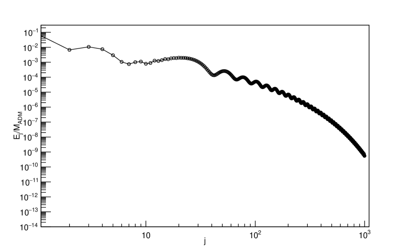
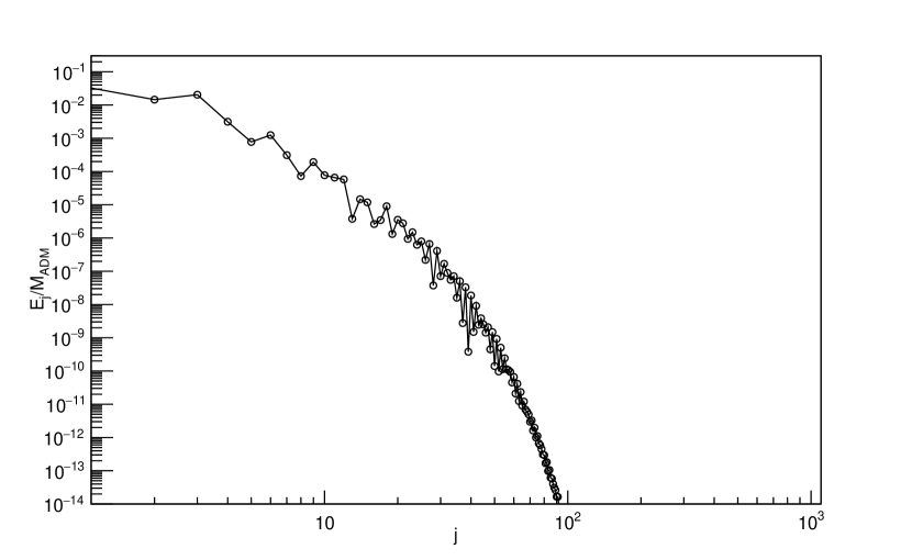
Finally, the time-evolved energy provides another possible measure of approximate thermalization in the dual CFT; namely, the spectrum should approach an (exponentially cut-off) power law at thermalization. In most cases, this occurs shortly before horizon formation, but there are exceptions, such as the late time behavior of initial data below the critical mass for black hole formation in Einstein-Gauss-Bonnet gravity Deppe et al. (2016). When there is evidence of chaotic behavior, it is particularly interesting to know if the spectra for similar amplitudes approach a power law at similar times even if horizons form at very different times. Figure 12 shows the energy spectra for two amplitudes in the chaotic region of the $t_{H}$ vs $\epsilon$ plot for $\mu=0,\sigma=1.1$. Figure 12(a) is the spectrum just before horizon formation for $\epsilon=1.01$, while figure 12(b) is the spectrum at approximately the same time for $\epsilon=1.02$, which is very long before horizon formation. In this example, we see that the spectrum does approach a power law for the evolution that is forming a horizon, while the other evolution demonstrates a more rapid decay (typically fit by a power law times an exponential in the literature). Therefore, this example suggests that a power law spectrum may yield similar results to horizon formation as a measure of thermalization in the dual CFT.

V Discussion

For the first time, we have presented the phase diagram of stability of AdS₅ against horizon formation, treating the scalar field mass $\mu$ and width $\sigma$ of initial data as free parameters. In addition to mapping the location of the so-called island of stability, we have gathered evidence for two non-perturbative classes on the shorelines of the island, the metastable and irregular classes. While these must either exhibit stability (no collapse below some critical amplitude) or instability (collapse at arbitrarily small but finite amplitude) as the amplitude $\epsilon\to 0$, they are distinguished by their behavior at computationally accessible (finite) amplitudes. While perturbatively unstable evolutions obey $t_{H}\propto\epsilon^{-2}$ as $\epsilon\to 0$ (and show evidence of this behavior at finite $\epsilon$), metastable initial data follows $t_{H}\propto\epsilon^{-p}$ for $p>2$ over a range of amplitudes $\epsilon>0$. The irregular class is characterized by horizon formation times $t_{H}$ that are not well described by a power law and sometimes exhibits non-monotonicity or even evidence of chaos. Both of these classes appear across the range of $\mu$ values that we study and at both small- and large-width boundaries of the stable class of initial data.

At this time, it is impossible to say whether metastable initial data are stable or unstable as $\epsilon\to 0$ (or if all metastable data behave in the same way in that limit). Our numerical evolutions include cases in which the lowest amplitudes jump either to metastable scaling with smaller $p$ or to evolutions that do not collapse over the time scales we study. We did find evidence that many metastable profiles move toward perturbatively unstable scaling ($t_{H}\propto\epsilon^{-2}$) as $\epsilon\to 0$ but more slowly than the initial data that we have classified as unstable. It is also possible that some metastable initial data are stable in the perturbative theory (ie, to $\epsilon^{3}$ order in a perturbative expansion) but not at higher orders. We emphasize once again, however, that our interest and therefore our classification is in small but finite $\epsilon$ behavior (which is by definition not strictly in the perturbative regime).

The irregular class seems likely to be (mostly) stable at arbitrarily small amplitudes based on our numerical evolutions, though we have not found a critical amplitude for monotonic irregular initial data. The irregular initial data includes the quasistable initial data described in Buchel et al. (2013); Deppe and Frey (2015), which has a sudden increase then decrease in $t_{H}$ as $\epsilon$ decreases as well as evidence for chaotic behavior. In fact, we have found evidence for weakly chaotic behavior for non-monotonic initial data in the form of a small but nonzero Lyapunov coefficient and in the phase space trajectory. Both non-monotonicity and chaos become stronger and more common at larger scalar masses; however, we have also found evidence of chaotic behavior for the massless scalar including in the $t_{H}$ vs $\epsilon$ curve. To our knowledge, this is the first evidence of chaos in this relationship for spherically symmetric massless scalar collapse in AdS, which is particularly interesting because there is only one physically meaningful ratio of scales, $\sigma$ as measured in AdS units.

While we have emphasized the appearance of new behaviors outside perturbation theory, metastable and irregular initial data are interesting potential subjects for analysis in the multiscale perturbation theory. A key question is if they demonstrate any unusual behavior there or map directly onto the stable or unstable classes.

Aside from the ultimate stability or instability of metastable and irregular initial data, several questions remain. For one, black holes formed in massive scalar collapse in asymptotically flat spacetime exhibit a mass gap for initial profiles wider than the Compton wavelength $1/\mu$ Brady et al. (1997). Whether this mass gap exists in AdS is not clear, and it may disappear through repeated gravitational focusing as the field oscillates many times across AdS; investigating this type of critical behavior will likely require techniques similar to those of Santos-Oliván and Sopuerta (2016). Returning to our stability phase diagram, the physical mechanism responsible for chaos that seems to occur for some irregular initial data is not yet clear. Is it some generalization of the same mechanism as found in the two-shell system? Also, would an alternate definition of approximate thermalization in the dual CFT, such as development of a power-law spectrum, lead to a different picture of the stability phase diagram? Finally, the big question is whether there is some test that could be performed on initial data alone that would predict in advance its behavior? So far, no test is entirely successful, so new ideas are necessary.

Appendix A Convergence Testing

Due to the large number of evolutions we have carried out, it is not computationally feasible to test all of them for convergence. Therefore, we have checked several interesting cases of irregular initial data, which are the most curious. These are carried out by evolving the initial data with a base resolution $n=14$ and again at $n=15,16$ with commensurate time steps, as described in Deppe and Frey (2015). In the cases indicated, we evaluated the order of convergence at lower resolutions. We remind the reader that the order of convergence $Q$ is the base-2 logarithm of the ratio of $L^{2}$ errors (root-mean-square over all corresponding grid points) between successive pairs of resolutions. We also note that the initial data are defined analytically, so $Q$ can appear poor at $t=0$ since the errors are controlled by round off; in some cases, $Q$ is therefore undefined and not plotted.

(a) $n=14$ base resolution

(b) $n=12$ base resolution

Figure 13: Convergence results for $\mu=0.5$, $\sigma=1$, $\epsilon=1.12$ showing order of convergence $Q$ vs time for $\phi,M,A,\delta$ (blue thin solid line, green dashed line, red dash-dotted line, cyan thick solid line, respectively). Left: Resolutions $n=14,15,16$ used. Right: Resolutions $n=12,13,14$ used.

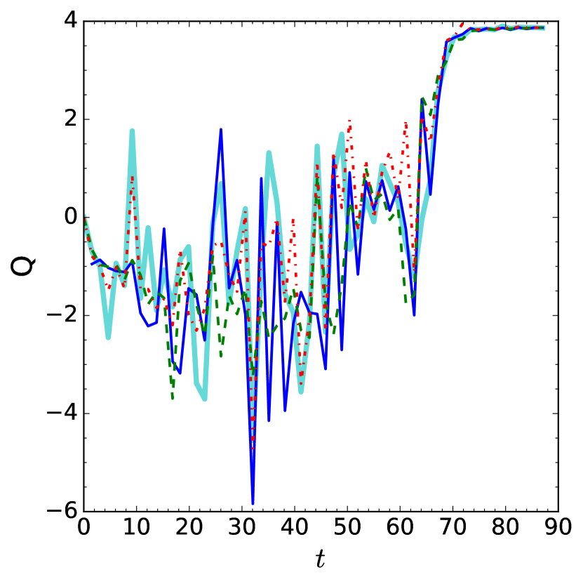
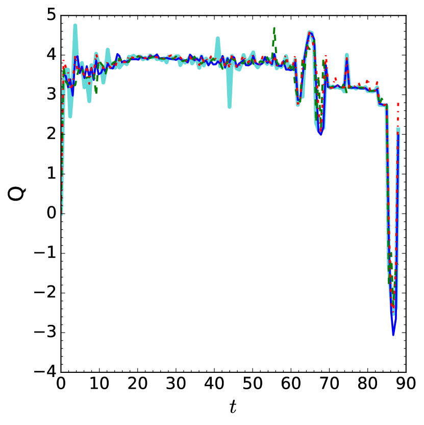
First, we carried out convergence tests for mass $\mu=0.5$, width $\sigma=1$, and amplitude $\epsilon=1.12$, which is monotonic irregular initial data presented in figure 5(a). This amplitude collapses with $t_{H}\sim 88$. Figure 13(a) shows the ($L^{2}$ norm) order of convergence for the field variable $\phi$, the mass function $M$, and the metric functions $A,\delta$. While the order of convergence is initially poor and even negative, all these variables show approximately fourth order convergence for times $t\gtrsim 70$. The reason for the initially poor convergence is that the error between successive resolutions is already given by (machine limited) round off. As a demonstration, we tested the order of convergence with base resolution $n=12$, as shown in figure 13(b). The variables show order of convergence $Q\gtrsim 3$ already at this resolution for most of the evolution, losing convergence only for $t>80$, where we see approximately 4th-order convergence in the $n=14$ resolution computations.

Two of the authors have discussed the convergence properties of evolution for the nonmonotonic irregular initial data with $\mu=20,\sigma=0.1,\epsilon=11.74$, which is in an amplitude region of increased $t_{H}$ surrounded by smaller values, in detail in Deppe and Frey (2015). In short, the variables $\phi,M,A,\delta$ all exhibit fourth order convergence, as does $\Pi^{2}(t,0)$, and the conserved mass actually has 6th order convergence.

(a) Horizon formation

(b) $\epsilon=7.42$

(c) $\epsilon=7.40$

Figure 14: Convergence results for $\mu=15$, $\sigma=0.2$. Left: $t_{H}$ vs $\epsilon$. Middle & Right: order of convergence vs time for $\phi,M,A,\delta$ (blue thin solid line, green dashed line, red dash-dotted line, cyan thick solid line, respectively) for indicated amplitudes.

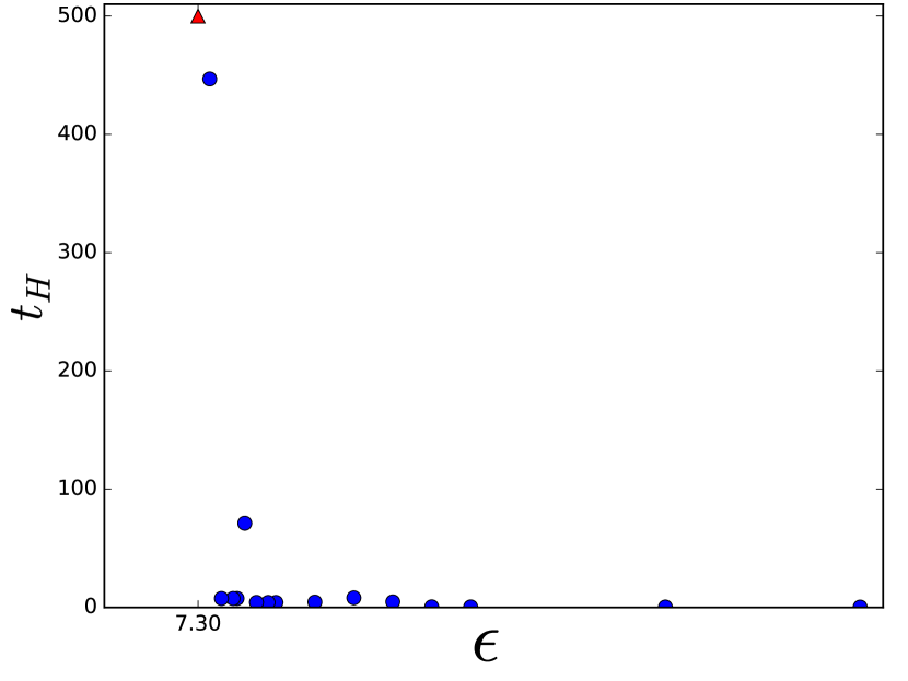
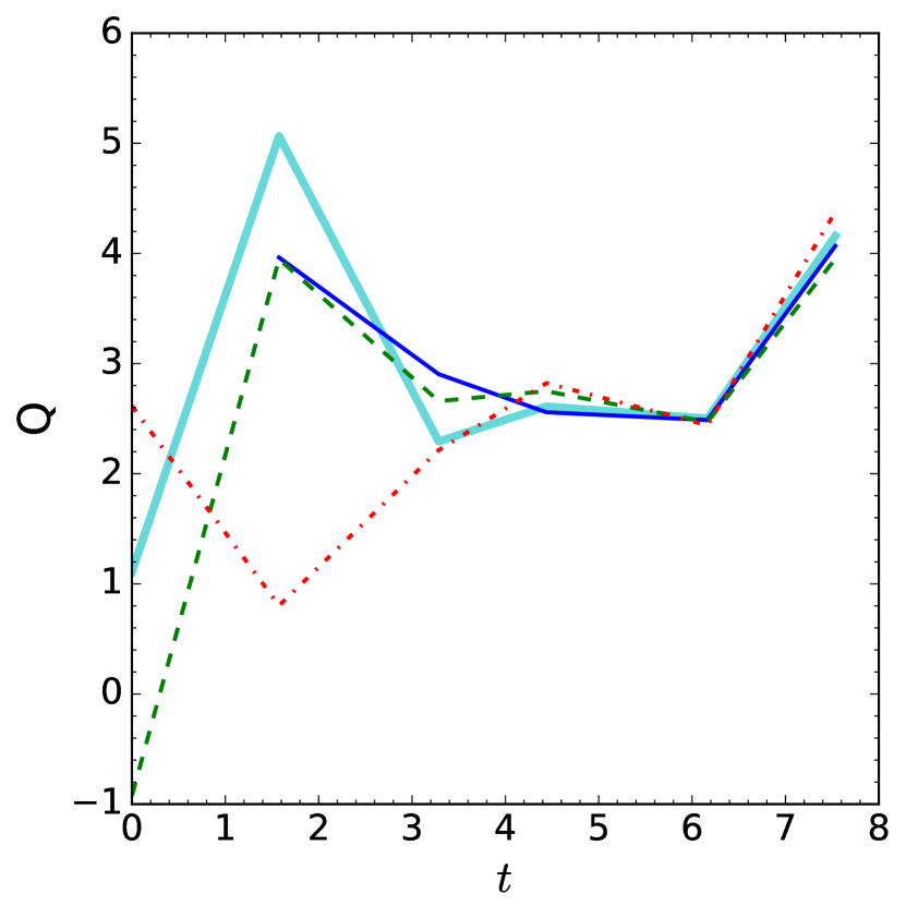
Initial data for $\mu=15,\sigma=0.2$ are also nonmonotonic, as shown in figure 14(a). While we have not analyzed all aspects of the convergence, we see from the remainder of figure 14 that $\phi,M,A,\delta$ exhibit convergent behavior at better than second order for $\epsilon=7.42$ (figure 14(b), second-largest value of $t_{H}$ in figure 14(a)) and $\epsilon=7.40$ (figure 14(c), adjacent amplitude in figure 14(a)). It is important to note that the larger amplitude also has the larger horizon formation time, contrary to the usual monotonic behavior. In other words, we have validated the nonmonotonicity of this initial data through convergence testing.

(a) $\epsilon=1.02$

(b) $\epsilon=1.01$

(c) $\epsilon=1.00$

Figure 15: Convergence results for $\mu=0$, $\sigma=1.1$ for listed amplitudes showing order of convergence $Q$ vs time for $\phi,M,A,\delta$ (blue thin solid line, green dashed line, red dash-dotted line, cyan thick solid line, respectively); resolutions $n=12,13,14$.

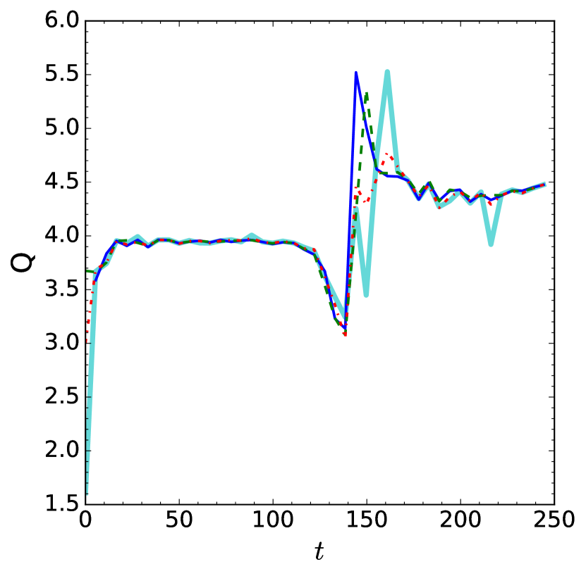
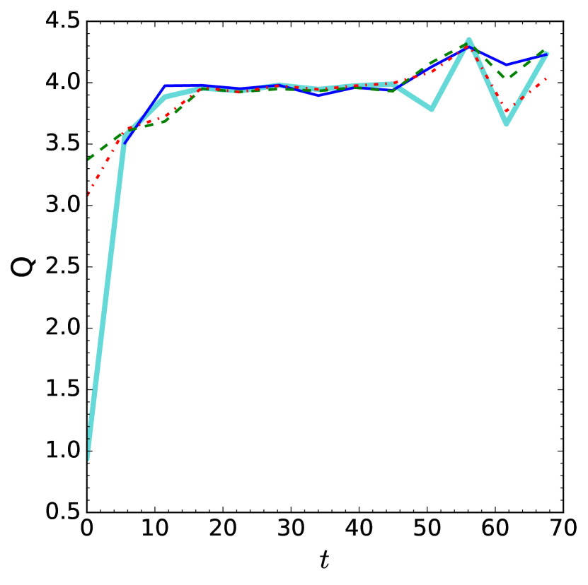
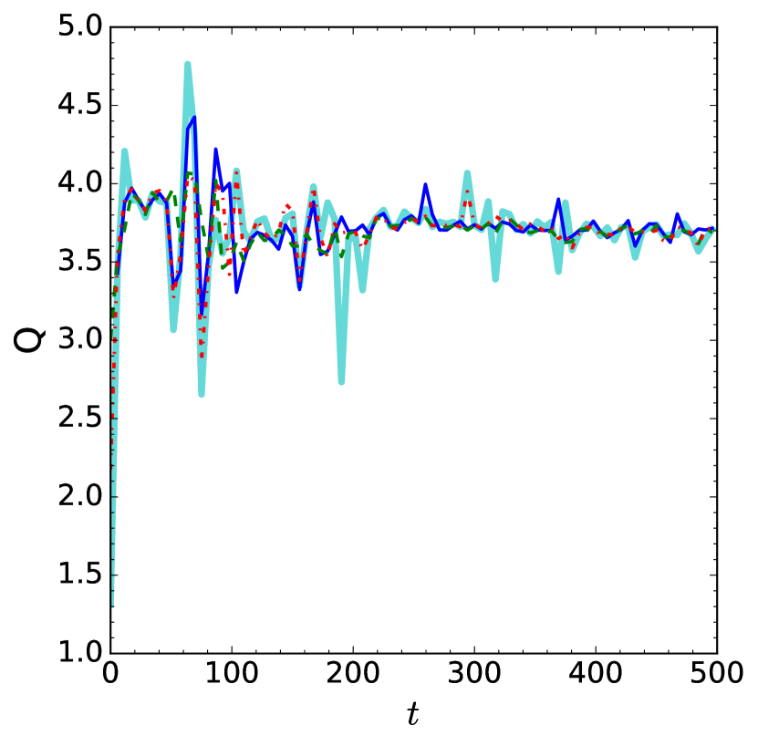
It is most crucial to validate the convergence of chaotic evolutions. In table 2, we noted that the Ricci scalar at the origin has nonzero Lyapunov exponent at almost the 2 sigma level for amplitudes $\epsilon=1.02,1.01,1.00$ for $\mu=0,\sigma=1.1$. We show the results of convergence tests for these amplitudes in figure 15; because these are longer evolutions, we consider the convergence at the lower resolutions $n=12,13,14$. After a transient start-up period, these are all convergent with $Q>2.5$ for all variables considered at all times; for most of the time, the order of convergence is $Q>3.5$. It is worth noting that one of the amplitudes does not form a horizon through $t=500$. These convergence tests validate both the nonmonotonic nature of the evolution ($t_{H}\approx 248,71$ and $>500$ for $\epsilon=1.02,1.01,1.00$ respectively) and also the calculation of the Lyapunov coefficient.

(a) $\epsilon=3.52$

(b) $\epsilon=3.51$

(c) $\epsilon=3.50$

Figure 16: Convergence results for $\mu=5$, $\sigma=0.34$ for listed amplitudes showing order of convergence $Q$ vs time for $\phi,M,A,\delta$ (blue thin solid line, green dashed line, red dash-dotted line, cyan thick solid line, respectively); resolutions $n=14,15,16$.

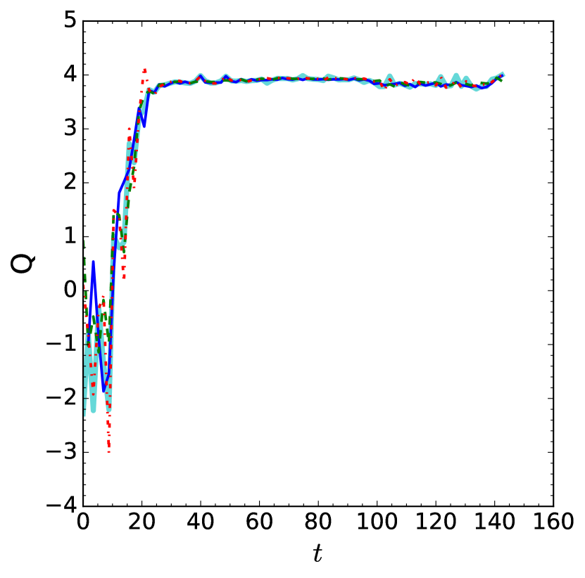
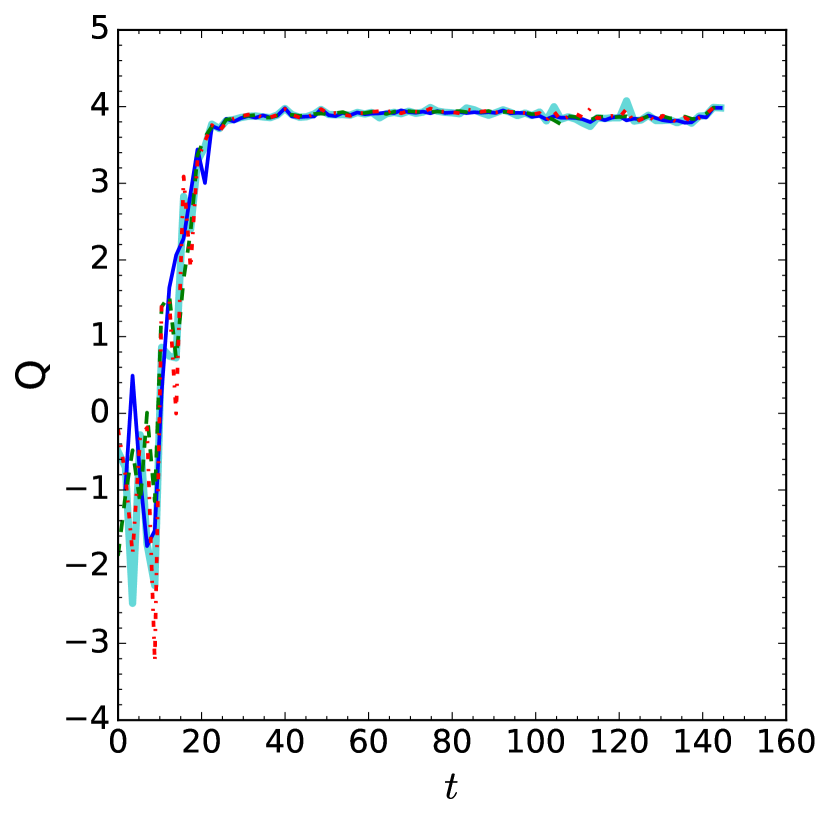
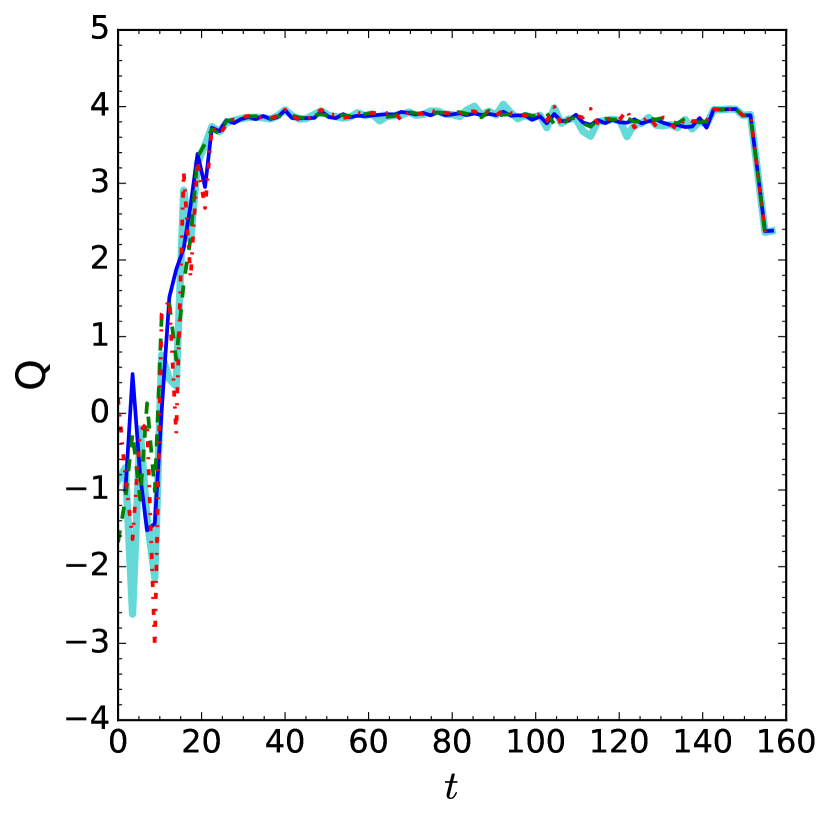
Also in table 2, we found a nonzero Lyapunov exponent for $\mu=5,\sigma=0.34$ at amplitudes $\epsilon=3.52,3.51,3.50$. The results of convergence tests for these amplitudes appear in figure 16. For $t\gtrsim 20$, these evolutions exhibit convergent behavior with $Q>3.5$ (and always $Q>2$). At early times, the apparent poor convergence is again due to the errors being dominated by round-off; we have carried out additional convergence tests (not shown) and verified that these evolutions are already convergent with order of convergence close to $Q=4$ at base resolutions $n=12$ for $t\lesssim 20$. Again, convergence tests validate chaotic behavior for these initial data.

(a) Horizon formation

(b) $\epsilon=1.15$

(c) $\epsilon=1.14$

Figure 17: Convergence results for $\mu=1$, $\sigma=1$. Left: $t_{H}$ vs $\epsilon$. Middle & Right: order of convergence $Q$ vs time for $\phi,M,A,\delta$ (blue thin solid line, green dashed line, red dash-dotted line, cyan thick solid line, respectively); resolutions $n=11,12,13$.

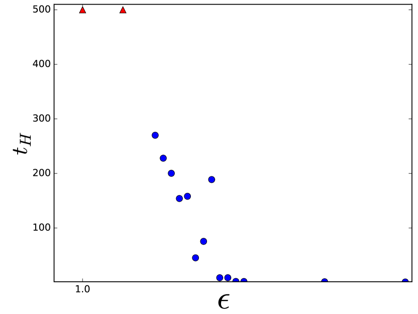
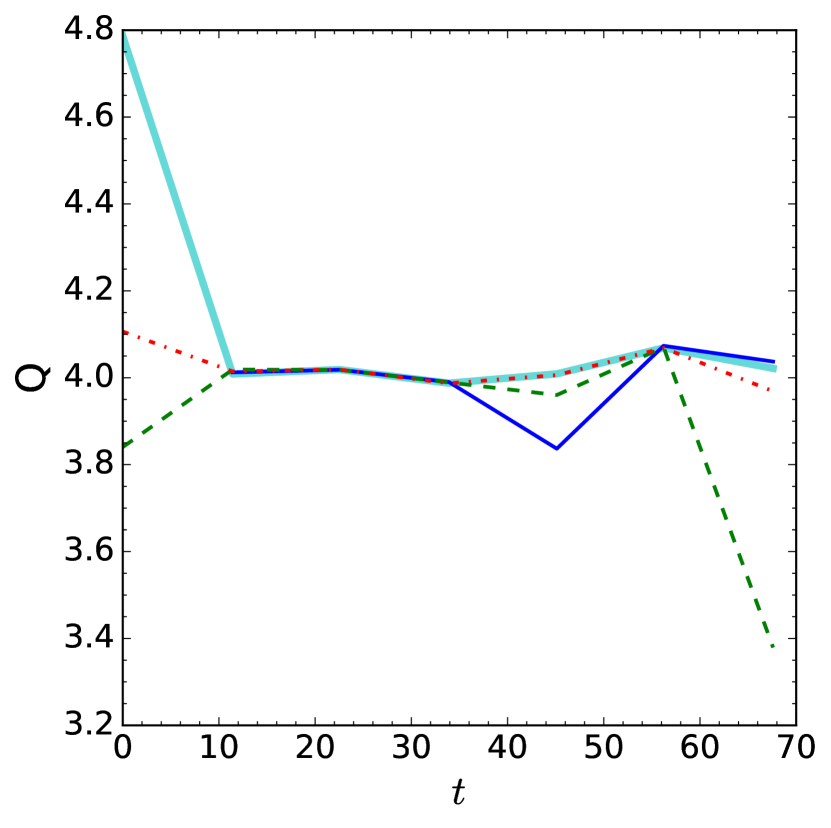
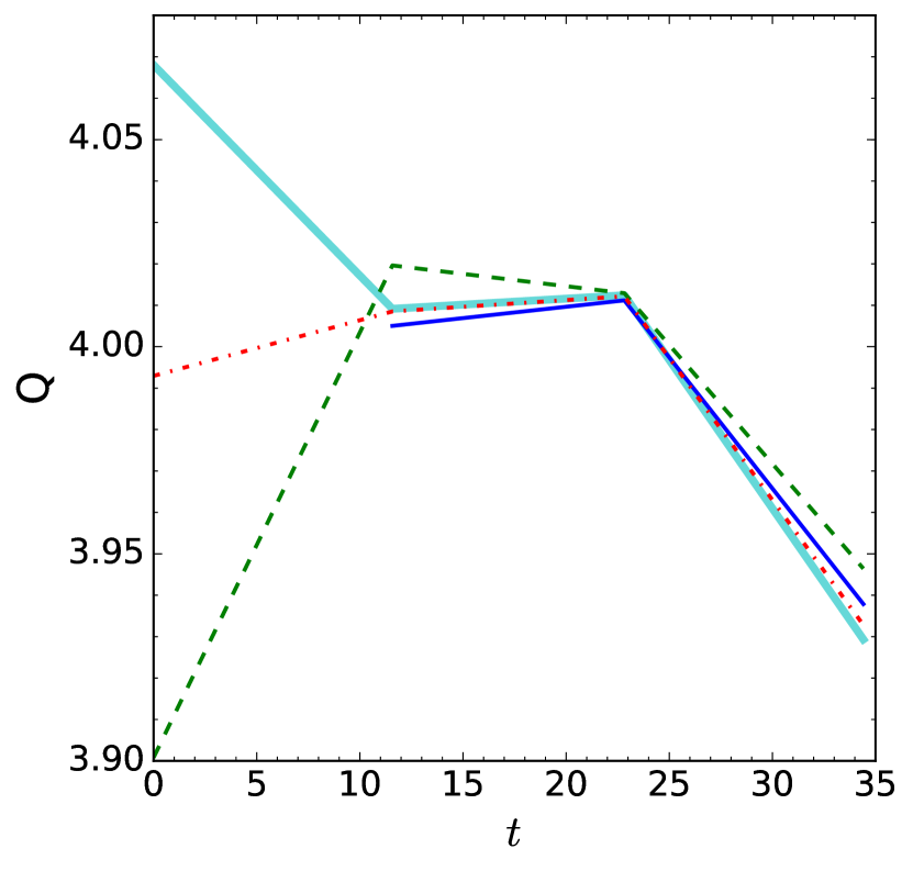
Initial data with $\mu=1,\sigma=1$ are chaotic over a narrow range of amplitudes. We have carried out convergence testing for amplitudes $\epsilon=1.15,1.14$, which are the two amplitudes with $t_{H}<100$ between amplitudes with $t_{H}\gtrsim 150$ in figure 17(a). The order of convergence was poor for these amplitudes in our initial tests with base resolution $n=14$ because the error between resolutions was dominated by round-off, similar to the convergence tests we discussed above for $\mu=0.5,\sigma=1$. In subsequent tests with lower resolutions $n=11,12,13$, we find an order of convergence $Q\sim 4$ for most of the evolutions (and always $Q>3$). It is important to note again that our evolutions exhibit convergence while showing horizon formation at a later time for a larger amplitude in this case, again validating the nonmonotonic behavior.

(a) $\epsilon=6.95$

(b) $\epsilon=6.92$

Figure 18: Order of convergence vs time for $\phi,M,A,\delta$ (blue thin solid line, green dashed line, red dash-dotted line, cyan thick solid line, respectively) for $\mu=20,\sigma=0.19$ and indicated amplitudes.

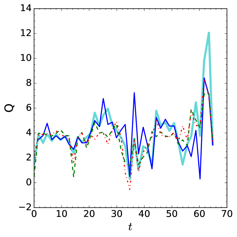
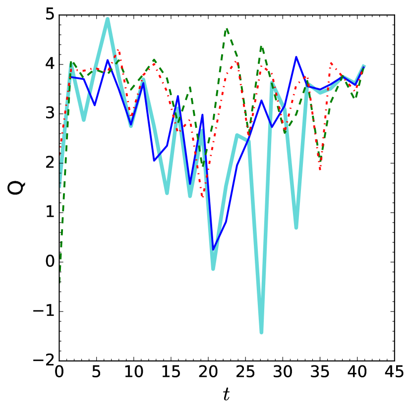
Finally, we ran convergence tests for the chaotic initial data with $\mu=20,\sigma=0.19$ for $\epsilon=6.95,6.92$, with $t_{H}\approx 65.5,40.8$ respectively. As shown in figure 18, the simulations are close to fourth order convergence for most of the evolution, but there are periods where the order of convergence for evolution and constraint variables becomes negative. This of course leads to the concern that the evolutions should have collapsed during those periods and extend into an “afterlife” evolution. We have therefore evolved these amplitudes through these regions (approximately $t=30-40$ for $\epsilon=6.95$ and $t=18-30$ for $\epsilon=6.92$) at high resolution ($n=18$). If the evolutions are truly in an afterlife, this higher resolution calculation may include horizon formation. We do not observe this. Another tell-tale of would-be horizon formation is a decrease in the time step size by an order of magnitude or more followed by an increase. We monitor the time step size every 500 time steps through this evolution but do not observe a decrease in time step size by more than a factor of 2. As a result, we believe the values of $t_{H}$ found are reliable, though the reader may wish to consider them with some caution. In other words, while convergence testing is the gold standard to validate our numerical evolutions, there are other indicators of reliability, which these evolutions satisfy. It is also worth noting that the rapid energy transfer characteristic of figure 11(d) for $\epsilon=6.95$ begins immediately and is therefore seen in a convergent region of the evolutions, particularly for $t\lesssim 14$.

Nonetheless, we emphasize that we have found convergent evolutions for irregular initial data at scalar masses from $\mu=0$ to $20$. It is important to note that we have validated nonmonotonic behavior in plots of $t_{H}$ vs $\epsilon$. Convergence testing also specifically validates the evolutions used to find a nonzero Lyapunov coefficient (at nearly the 2$\sigma$ level) for massless scalar collapse.

References

- Bizon and Rostworowski (2011) Piotr Bizon and Andrzej Rostworowski, “On weakly turbulent instability of anti-de Sitter space,” Phys. Rev. Lett. 107, 031102 (2011), arXiv:1104.3702 [gr-qc] .
- Garfinkle and Pando Zayas (2011) David Garfinkle and Leopoldo A. Pando Zayas, “Rapid Thermalization in Field Theory from Gravitational Collapse,” Phys. Rev. D84, 066006 (2011), arXiv:1106.2339 [hep-th] .
- Jalmuzna et al. (2011) Joanna Jalmuzna, Andrzej Rostworowski, and Piotr Bizon, “A Comment on AdS collapse of a scalar field in higher dimensions,” Phys. Rev. D84, 085021 (2011), arXiv:1108.4539 [gr-qc] .
- Garfinkle et al. (2012) David Garfinkle, Leopoldo A. Pando Zayas, and Dori Reichmann, “On Field Theory Thermalization from Gravitational Collapse,” JHEP 02, 119 (2012), arXiv:1110.5823 [hep-th] .
- Dias et al. (2012) Oscar J. C. Dias, Gary T. Horowitz, and Jorge E. Santos, “Gravitational Turbulent Instability of Anti-de Sitter Space,” Class. Quant. Grav. 29, 194002 (2012), arXiv:1109.1825 [hep-th] .
- Balasubramanian et al. (2014) Venkat Balasubramanian, Alex Buchel, Stephen R. Green, Luis Lehner, and Steven L. Liebling, “Holographic Thermalization, Stability of Anti–de Sitter Space, and the Fermi-Pasta-Ulam Paradox,” Phys. Rev. Lett. 113, 071601 (2014), arXiv:1403.6471 [hep-th] .
- Craps et al. (2014) Ben Craps, Oleg Evnin, and Joris Vanhoof, “Renormalization group, secular term resummation and AdS (in)stability,” JHEP 10, 048 (2014), arXiv:1407.6273 [gr-qc] .
- Basu et al. (2015) Pallab Basu, Chethan Krishnan, and Ayush Saurabh, “A stochasticity threshold in holography and the instability of AdS,” Int. J. Mod. Phys. A30, 1550128 (2015), arXiv:1408.0624 [hep-th] .
- Dimitrakopoulos et al. (2015) Fotios V. Dimitrakopoulos, Ben Freivogel, Matthew Lippert, and I-Sheng Yang, “Position space analysis of the AdS (in)stability problem,” JHEP 08, 077 (2015), arXiv:1410.1880 [hep-th] .
- Buchel et al. (2015) Alex Buchel, Stephen R. Green, Luis Lehner, and Steve L. Liebling, “Conserved quantities and dual turbulent cascades in anti–de Sitter spacetime,” Phys. Rev. D91, 064026 (2015), arXiv:1412.4761 [gr-qc] .
- Craps et al. (2015a) Ben Craps, Oleg Evnin, and Joris Vanhoof, “Renormalization, averaging, conservation laws and AdS (in)stability,” JHEP 01, 108 (2015a), arXiv:1412.3249 [gr-qc] .
- Evnin and Krishnan (2015) Oleg Evnin and Chethan Krishnan, “A Hidden Symmetry of AdS Resonances,” Phys. Rev. D91, 126010 (2015), arXiv:1502.03749 [hep-th] .
- Dimitrakopoulos and Yang (2015) Fotios Dimitrakopoulos and I-Sheng Yang, “Conditionally extended validity of perturbation theory: Persistence of AdS stability islands,” Phys. Rev. D92, 083013 (2015), arXiv:1507.02684 [hep-th] .
- Green et al. (2015) Stephen R. Green, Antoine Maillard, Luis Lehner, and Steven L. Liebling, “Islands of stability and recurrence times in AdS,” Phys. Rev. D92, 084001 (2015), arXiv:1507.08261 [gr-qc] .
- Craps et al. (2015b) Ben Craps, Oleg Evnin, and Joris Vanhoof, “Ultraviolet asymptotics and singular dynamics of AdS perturbations,” JHEP 10, 079 (2015b), arXiv:1508.04943 [gr-qc] .
- Craps et al. (2015c) Ben Craps, Oleg Evnin, Puttarak Jai-akson, and Joris Vanhoof, “Ultraviolet asymptotics for quasiperiodic AdS4 perturbations,” JHEP 10, 080 (2015c), arXiv:1508.05474 [gr-qc] .
- Craps and Evnin (2016) Ben Craps and Oleg Evnin, “AdS (in)stability: an analytic approach,” Proceedings, The String Theory Universe, 21st European String Workshop and 3rd COST MP1210 Meeting: Leuven, Belgium, September 7-11, 2015, Fortsch. Phys. 64, 336–344 (2016), arXiv:1510.07836 [gr-qc] .
- Buchel et al. (2013) Alex Buchel, Steven L. Liebling, and Luis Lehner, “Boson stars in AdS spacetime,” Phys. Rev. D87, 123006 (2013), arXiv:1304.4166 [gr-qc] .
- Maliborski and Rostworowski (2013a) Maciej Maliborski and Andrzej Rostworowski, “A comment on ”Boson stars in AdS”,” (2013a), arXiv:1307.2875 [gr-qc] .
- Maliborski and Rostworowski (2013b) Maciej Maliborski and Andrzej Rostworowski, “Lecture Notes on Turbulent Instability of Anti-de Sitter Spacetime,” Proceedings, Spring School on Numerical Relativity and High Energy Physics (NR/HEP2): Lisbon, Portugal, March 11-14, 2013, Int. J. Mod. Phys. A28, 1340020 (2013b), arXiv:1308.1235 [gr-qc] .
- Bizoń and Rostworowski (2015) Piotr Bizoń and Andrzej Rostworowski, “Comment on “Holographic Thermalization, Stability of Anti–de Sitter Space, and the Fermi-Pasta-Ulam Paradox”,” Phys. Rev. Lett. 115, 049101 (2015), arXiv:1410.2631 [gr-qc] .
- Balasubramanian et al. (2015) Venkat Balasubramanian, Alex Buchel, Stephen R. Green, Luis Lehner, and Steven L. Liebling, “Reply to Comment on “Holographic Thermalization, Stability of Anti–de Sitter Space, and the Fermi-Pasta-Ulam Paradox”,” Phys. Rev. Lett. 115, 049102 (2015), arXiv:1506.07907 [gr-qc] .
- Bizoń et al. (2015) Piotr Bizoń, Maciej Maliborski, and Andrzej Rostworowski, “Resonant Dynamics and the Instability of Anti–de Sitter Spacetime,” Phys. Rev. Lett. 115, 081103 (2015), arXiv:1506.03519 [gr-qc] .
- Deppe (2019) Nils Deppe, “Resonant dynamics in higher dimensional anti–de Sitter spacetime,” Phys. Rev. D 100, 124028 (2019), arXiv:1606.02712 [gr-qc] .
- Dimitrakopoulos et al. (2016) Fotios V. Dimitrakopoulos, Ben Freivogel, Juan F. Pedraza, and I-Sheng Yang, “Gauge dependence of the AdS instability problem,” Phys. Rev. D94, 124008 (2016), arXiv:1607.08094 [hep-th] .
- Dimitrakopoulos et al. (2018) Fotios V. Dimitrakopoulos, Ben Freivogel, and Juan F. Pedraza, “Fast and Slow Coherent Cascades in Anti-de Sitter Spacetime,” Class. Quant. Grav. 35, 125008 (2018), arXiv:1612.04758 [hep-th] .
- Liebling and Khanna (2017) Steven L. Liebling and Gaurav Khanna, “Scalar collapse in AdS with an OpenCL open source code,” Class. Quant. Grav. 34, 205012 (2017), arXiv:1706.07413 [gr-qc] .
- Bizoń and Jałmużna (2013) Piotr Bizoń and Joanna Jałmużna, “Globally regular instability of ,” Phys. Rev. Lett. 111, 041102 (2013), arXiv:1306.0317 [gr-qc] .
- da Silva et al. (2015) Emilia da Silva, Esperanza Lopez, Javier Mas, and Alexandre Serantes, “Collapse and Revival in Holographic Quenches,” JHEP 04, 038 (2015), arXiv:1412.6002 [hep-th] .
- Deppe et al. (2016) Nils Deppe, Allison Kolly, Andrew R. Frey, and Gabor Kunstatter, “Black Hole Formation in AdS Einstein-Gauss-Bonnet Gravity,” JHEP 10, 087 (2016), arXiv:1608.05402 [hep-th] .
- Deppe et al. (2015) Nils Deppe, Allison Kolly, Andrew Frey, and Gabor Kunstatter, “Stability of AdS in Einstein Gauss Bonnet Gravity,” Phys. Rev. Lett. 114, 071102 (2015), arXiv:1410.1869 [hep-th] .
- Arias et al. (2016) Raúl Arias, Javier Mas, and Alexandre Serantes, “Stability of charged global AdS4 spacetimes,” JHEP 09, 024 (2016), arXiv:1606.00830 [hep-th] .
- Okawa et al. (2015) Hirotada Okawa, Jorge C. Lopes, and Vitor Cardoso, “Collapse of massive fields in anti-de Sitter spacetime,” (2015), arXiv:1504.05203 [gr-qc] .
- Deppe and Frey (2015) Nils Deppe and Andrew R. Frey, “Classes of Stable Initial Data for Massless and Massive Scalars in Anti-de Sitter Spacetime,” JHEP 12, 004 (2015), arXiv:1508.02709 [hep-th] .
- Hubeny and Rangamani (2002) Veronika E. Hubeny and Mukund Rangamani, “Unstable horizons,” JHEP 05, 027 (2002), arXiv:hep-th/0202189 [hep-th] .
- Buchel and Lehner (2015) Alex Buchel and Luis Lehner, “Small black holes in ,” Class. Quant. Grav. 32, 145003 (2015), arXiv:1502.01574 [hep-th] .
- Buchel (2017) Alex Buchel, “Universality of small black hole instability in AdS/CFT,” Int. J. Mod. Phys. D26, 1750140 (2017), arXiv:1509.07780 [hep-th] .
- Buchel and Buchel (2015) Alex Buchel and Michael Buchel, “On stability of nonthermal states in strongly coupled gauge theories,” (2015), arXiv:1509.00774 [hep-th] .
- Brito et al. (2016) Richard Brito, Vitor Cardoso, and Jorge V. Rocha, “Interacting shells in AdS spacetime and chaos,” Phys. Rev. D94, 024003 (2016), arXiv:1602.03535 [hep-th] .
- de Oliveira et al. (2012) H. P. de Oliveira, Leopoldo A. Pando Zayas, and Cesar A. Terrero-Escalante, “Turbulence and Chaos in Anti-de-Sitter Gravity,” Int. J. Mod. Phys. D21, 1242013 (2012), arXiv:1205.3232 [hep-th] .
- Aharony et al. (2000) Ofer Aharony, Steven S. Gubser, Juan Martin Maldacena, Hirosi Ooguri, and Yaron Oz, “Large N field theories, string theory and gravity,” Phys. Rept. 323, 183–386 (2000), arXiv:hep-th/9905111 [hep-th] .
- Nastase (2015) Horatiu Nastase, Introduction to the ADS/CFT Correspondence (Cambridge University Press, 2015).
- Brady et al. (1997) Patrick R. Brady, Chris M. Chambers, and Sergio M. C. V. Goncalves, “Phases of massive scalar field collapse,” Phys. Rev. D56, 6057–6061 (1997), arXiv:gr-qc/9709014 [gr-qc] .
- Santos-Oliván and Sopuerta (2016) Daniel Santos-Oliván and Carlos F. Sopuerta, “Moving closer to the collapse of a massless scalar field in spherically symmetric anti–de Sitter spacetimes,” Phys. Rev. D93, 104002 (2016), arXiv:1603.03613 [gr-qc] .