Infimal convolution of oscillation total generalized variation for the recovery of images with structured texture

Yiming Gao Department of Mathematics, Nanjing University of Science and Technology, 210094 Nanjing, Jiangsu, China. Email: gao_yiming@hotmail.com.    Kristian Bredies Institute of Mathematics and Scientific Computing, University of Graz, Heinrichstraße 36, A-8010 Graz, Austria. Email: kristian.bredies@uni-graz.at. The Institute for Mathematics and Scientific Computing is a member of NAWI Graz (http://www.nawigraz.at/).
Abstract:

We propose a new type of regularization functional for images called oscillation total generalized variation (TGV) which can represent structured textures with oscillatory character in a specified direction and scale. The infimal convolution of oscillation TGV with respect to several directions and scales is then used to model images with structured oscillatory texture. Such functionals constitute a regularizer with good texture preservation properties and can flexibly be incorporated into many imaging problems. We give a detailed theoretical analysis of the infimal-convolution-type model with oscillation TGV in function spaces. Furthermore, we consider appropriate discretizations of these functionals and introduce a first-order primal-dual algorithm for solving general variational imaging problems associated with this regularizer. Finally, numerical experiments are presented which show that our proposed models can recover textures well and are competitive in comparison to existing state-of-the-art methods.

Mathematics subject classification:

94A08, 68U10, 26A45, 90C90.

Key words:

Oscillation total generalized variation, infimal-convolution-type regularization, texture modeling, cartoon/texture decomposition, image denoising, image inpainting, undersampled magnetic resonance imaging.

1 Introduction

After the introduction of total variation (TV) to image processing [46], variational models were developed for a wide range of applications in imaging during the last decades. In that context, variational models that base on image decomposition have also become increasingly popular. The concept of these models is to decompose an image into two or more components which inherit distinguishing characteristics. The classical TV (ROF) model for image denoising can, for instance, be regarded as a decomposition model:

minuBV(Ω),vL2(Ω)u+v=fλ2v2+J(u),subscriptformulae-sequence𝑢BVΩ𝑣superscript𝐿2Ω𝑢𝑣𝑓𝜆2superscriptnorm𝑣2𝐽𝑢\min_{\begin{subarray}{c}u\in\operatorname{BV}(\Omega),\ v\in L^{2}(\Omega)\\ u+v=f\end{subarray}}\ \frac{\lambda}{2}\|{v}\|^{2}+J(u), (1)

where f𝑓f is the observed noisy image, J(u)=Ω|Du|𝐽𝑢subscriptΩ𝐷𝑢J(u)=\int_{\Omega}|Du| is the total variation, i.e., the Radon norm of the distributional derivative, and \|\cdot\| represents the L2superscript𝐿2L^{2} norm, both associated with a bounded domain ΩdΩsuperscript𝑑\Omega\subset\mathbb{R}^{d}. In such an approach, we decompose the image to a noise-free image component u𝑢u belonging to BV(Ω)BVΩ\operatorname{BV}(\Omega) and a noise or small-scale texture component in L2(Ω)superscript𝐿2ΩL^{2}(\Omega). In [42], Y. Meyer pointed out some limitations of the above model and introduced a new space G(Ω)=W1,(Ω)𝐺Ωsuperscript𝑊1ΩG(\Omega)=W^{-1,\infty}(\Omega), which is larger than L2(Ω)superscript𝐿2ΩL^{2}(\Omega), to model oscillating patterns that are typical for structured texture:

minuBV(Ω),vG(Ω)u+v=fλvG+J(u),subscriptformulae-sequence𝑢BVΩ𝑣𝐺Ω𝑢𝑣𝑓𝜆subscriptnorm𝑣𝐺𝐽𝑢\min_{\begin{subarray}{c}u\in\operatorname{BV}(\Omega),\ v\in G(\Omega)\\ u+v=f\end{subarray}}\lambda\|{v}\|_{G}+J(u), (2)

where G(Ω)𝐺ΩG(\Omega) denotes the space G(Ω)={v=divg:g=(g1,,gd)L(Ω)d}𝐺Ωconditional-set𝑣div𝑔𝑔subscript𝑔1subscript𝑔𝑑superscript𝐿superscriptΩ𝑑G(\Omega)=\{v=\operatorname{div}g:g=(g_{1},\ldots,g_{d})\in L^{\infty}(\Omega)^{d}\} with the norm vG=inf{g:v=divg,g=(g1,,gd)L(Ω)d}\|v\|_{G}=\inf\ \{\|g\|_{\infty}:v=\operatorname{div}g,g=(g_{1},\ldots,g_{d})\in L^{\infty}(\Omega)^{d}\} and again, J(u)=Ω|Du|𝐽𝑢subscriptΩ𝐷𝑢J(u)=\int_{\Omega}|{Du}|. In this model, u𝑢u represents a piecewise constant function, consisting of homogeneous regions with sharp boundaries and is usually called cartoon component. The other part v𝑣v in G(Ω)𝐺ΩG(\Omega) contains oscillating patterns, like textures and noise. This model can be considered as the original cartoon-texture decomposition model. However, the G𝐺G-space may be difficult to handle in implementations. Vese and Osher [52] approximated the G𝐺G-space by a Sobolev space of negative differentiability order W1,p(Ω)superscript𝑊1𝑝ΩW^{-1,p}(\Omega), which can, in practice, more easily be implemented by partial differential equations. Later, Aujol et al. [4] made a modification to the G𝐺G-norm term in (2) which is replaced by constraining v𝑣v to the set Gμ(Ω)={vG(Ω):vGμ}subscript𝐺𝜇Ωconditional-set𝑣𝐺Ωsubscriptnorm𝑣𝐺𝜇G_{\mu}(\Omega)=\{v\in G(\Omega):\|v\|_{G}\leq\mu\}. As a consequence, the problem can be solved alternatingly by Chambolle’s projection method [23] with respect to the two variables u𝑢u and v𝑣v.

Certainly, the aim of above models is to find an appropriate norm to describe textures. However, in general, the above norms can represent all kinds of oscillatory parts. As a consequence, since noise can be regarded as small-scale oscillating texture, these models do not deal well with noise. In order to tackle this disadvantage, in [47], Schaeffer and Osher incorporated robust principal component analysis (PCA) [22] into cartoon-texture decomposition models based on the patch method. For the texture part, the authors suggest to decompose the image into small, non-overlapping patches, written as vectors. The collection of the patch vectors is assumed to be (highly) linearly dependent and thus to have low rank. This suggests to minimize the nuclear norm of the patch-vector matrix. However, the choice of the block-size of the patches for this model is challenging and also, the numerical optimization procedures for the associated functionals have to rely on computationally expensive matrix-decomposition methods such as singular-value thresholding, for instance. Alternatively, rather than considering the cartoon and texture components separately, another efficient texture preservation approach is using non-local methods which is also based on patches. For more details, we refer readers to [15, 16, 30, 53]. Furthermore, in order to enhance and reconstruct line structures well, Holler and Kunisch [33] proposed an infimal convolution of TGV-type (ICTGV) functionals which can capture some directional line textures. Disadvantages are, of course, the bias of this regularization approach towards certain directions and the fact that we cannot expect to recover texture that is not composed of different line structures. In [38], Kongskov and Dong proposed a new directional total generalized variation (DTGV) functional to capture the directional information of an image, which can be considered as a special case of ICTGV.

Another approach to decompose an image is to compute sparse representations based on dictionaries. The basic idea is to find two suitable dictionaries, one adapted to represent textures, and the other to represent the cartoon part. In the papers [27, 49], Elad et al. combined the basis pursuit denoising (BPDN) algorithm and the TV-regularization scheme to the following decomposition model:

minαt,αnαt1+αn1+λ2fTtαtTnαn2+γJ(Tnαn),subscriptsubscript𝛼tsubscript𝛼nsubscriptnormsubscript𝛼t1subscriptnormsubscript𝛼n1𝜆2superscriptnorm𝑓subscript𝑇tsubscript𝛼tsubscript𝑇nsubscript𝛼n2𝛾𝐽subscript𝑇nsubscript𝛼n\min_{\alpha_{\mathrm{t}},\alpha_{\mathrm{n}}}\|\alpha_{\mathrm{t}}\|_{1}+\|\alpha_{\mathrm{n}}\|_{1}+\frac{\lambda}{2}\|f-T_{\mathrm{t}}\alpha_{\mathrm{t}}-T_{\mathrm{n}}\alpha_{\mathrm{n}}\|^{2}+\gamma J(T_{\mathrm{n}}\alpha_{\mathrm{n}}), (3)

where Tt,Tnsubscript𝑇tsubscript𝑇nT_{\mathrm{t}},T_{\mathrm{n}} are dictionary synthesis operators for the texture and cartoon parts αt,αnsubscript𝛼tsubscript𝛼n\alpha_{\mathrm{t}},\alpha_{\mathrm{n}}, respectively, and J𝐽J is again the total variation. Penalizing with TV forces the cartoon content Tnαnsubscript𝑇nsubscript𝛼nT_{\mathrm{n}}\alpha_{\mathrm{n}} to have a sparser gradient and to be closer to a piecewise constant image. Here, the choice of the dictionary synthesis operators Tt,Tnsubscript𝑇tsubscript𝑇nT_{\mathrm{t}},T_{\mathrm{n}} is the main challenge for this approach. The best choice for one image depends on experience and may be not suitable for another image with different structures. The authors recommended that for the texture content, one may use local discrete cosine transform (DCT) or the Gabor transform, and for the cartoon content one may use curvelet, ridgelets, contourlets and so on. This approach is reported to perform well for the restoration of texture images [27, 49]. Inspired by this, Cai, Osher and Shen [21] constructed a cartoon-texture model with tight framelets [20] and local DCT which can easily be realized algorithmically by split Bregman iterations.

Recently, filtering approaches have been widely used in image decomposition. Gilboa et al. proposed a generalization of the structure-texture decomposition method based on TV scale space which is also known as TV flow in [28, 29, 34]. The aim is to construct a TV spectral framework to analyze dominant features in the transform domain, filter in that domain, and then perform an inverse transform back to the spatial domain to obtain the filtered response. In [19], Burger et al. extended this notion to general one-homogeneous functionals, not only TV regularization. Furthermore, Buades et al. proposed a non-linear filter that decomposes the image into a geometric and an oscillatory part in [17, 18], in which a non-linear low-high frequency decomposition is computed by using isotropic filters. However, the cartoon parts produced by these filters are not well-structured and textures also contain other oscillatory components. Furthermore, these methods are not variational models and can not easily be transferred to other image processing problems such as solving inverse problems, for instance.

In this paper, we propose a new regularization which can represent structured texture that consists of different directions and frequencies. The regularization is called oscillation total generalized variation (oscillation TGV) and defined as follows:

TGVα,β,𝐜osci(u)=minwBD(Ω)αuw+βw+𝐜u,for uL1(Ω),subscriptsuperscriptTGVosci𝛼𝛽𝐜𝑢subscript𝑤BDΩ𝛼subscriptnorm𝑢𝑤𝛽subscriptnorm𝑤𝐜𝑢for uL1(Ω)\operatorname{TGV}^{\operatorname{osci}}_{\alpha,\beta,\mathbf{c}}(u)=\min_{w\in\text{BD}(\Omega)}\alpha\|\nabla u-w\|_{\mathcal{M}}+\beta\|\mathcal{E}w+\mathbf{c}u\|_{\mathcal{M}},\quad\text{for $u\in L^{1}(\Omega)$}, (4)

where α,β>0𝛼𝛽0\alpha,\beta>0, BD(Ω)BDΩ\operatorname{BD}(\Omega) denotes the space of vector fields of bounded deformation, the operator \nabla denotes the weak derivative, the operator \mathcal{E} is the weak symmetrized derivative w=12(w+wT)𝑤12𝑤superscript𝑤𝑇\mathcal{E}w=\frac{1}{2}(\nabla w+\nabla w^{T}) and \|\cdot\|_{\mathcal{M}} is the Radon norm. Moreover, 𝐜d×d𝐜superscript𝑑𝑑\mathbf{c}\in\mathbb{R}^{d\times d} and 𝐜u𝐜𝑢\mathbf{c}u corresponds to the matrix field given by (𝐜u)ij=cijusubscript𝐜𝑢𝑖𝑗subscript𝑐𝑖𝑗𝑢(\mathbf{c}u)_{ij}=c_{ij}u for i,j=1,,dformulae-sequence𝑖𝑗1𝑑i,j=1,\ldots,d. In (4), we set 𝐜=ωω𝐜tensor-product𝜔𝜔\mathbf{c}=\omega\otimes\omega for some ωd𝜔superscript𝑑\omega\in\mathbb{R}^{d}, i.e., cij=ωiωjsubscript𝑐𝑖𝑗subscript𝜔𝑖subscript𝜔𝑗c_{ij}=\omega_{i}\omega_{j}. For a precise description of these notions, we ask for the reader’s patience until Section 2. This regularization functional reduces to the original second-order TGV functional when 𝐜=0𝐜0\mathbf{c}=0, i.e.,

TGVα,β2(u)=minwBD(Ω)αuw+βw,superscriptsubscriptTGV𝛼𝛽2𝑢subscript𝑤BDΩ𝛼subscriptnorm𝑢𝑤𝛽subscriptnorm𝑤\operatorname{TGV}_{\alpha,\beta}^{2}(u)=\min_{w\in\operatorname{BD}(\Omega)}\alpha\|{\nabla u-w}\|_{\mathcal{M}}+\beta\|{\mathcal{E}w}\|_{\mathcal{M}}, (5)

which has been widely-used in imaging applications, such as, for instance, denoising, (dynamic) MRI and QSM reconstruction, diffusion tensor image restoration, JPEG and MPEG decompression, zooming, optical flow estimation [9, 10, 8, 11, 12, 14, 33, 35, 37, 39, 44, 48, 51], and many more. Furthermore, we consider m𝑚m-fold infimal convolution of oscillation TGV:

ICTGVα,β,𝐜osci(u)subscriptsuperscriptICTGVosci𝛼𝛽𝐜𝑢\displaystyle\operatorname{ICTGV}^{\operatorname{osci}}_{\vec{\alpha},\vec{\beta},\vec{\mathbf{c}}}(u) =(TGVα1,β1,𝐜1osciTGVαm,βm,𝐜mosci)(u)absentsubscriptsuperscriptTGVoscisubscript𝛼1subscript𝛽1subscript𝐜1subscriptsuperscriptTGVoscisubscript𝛼𝑚subscript𝛽𝑚subscript𝐜𝑚𝑢\displaystyle=(\operatorname{TGV}^{\operatorname{osci}}_{\alpha_{1},\beta_{1},\mathbf{c}_{1}}\hskip 0.83328pt\Box\hskip 0.83328pt\ldots\hskip 0.83328pt\Box\hskip 0.83328pt\operatorname{TGV}^{\operatorname{osci}}_{\alpha_{m},\beta_{m},\mathbf{c}_{m}})(u)
=infu1++um=ui=1mTGVαi,βi,𝐜iosci(ui)absentsubscriptinfimumsubscript𝑢1subscript𝑢𝑚𝑢superscriptsubscript𝑖1𝑚subscriptsuperscriptTGVoscisubscript𝛼𝑖subscript𝛽𝑖subscript𝐜𝑖subscript𝑢𝑖\displaystyle=\inf_{u_{1}+\ldots+u_{m}=u}\ \sum_{i=1}^{m}\operatorname{TGV}^{\operatorname{osci}}_{\alpha_{i},\beta_{i},\mathbf{c}_{i}}(u_{i}) (6)

where α=(α1,αm)𝛼subscript𝛼1subscript𝛼𝑚\vec{\alpha}=(\alpha_{1}\ldots,\alpha_{m}), β=(β1,,βm)𝛽subscript𝛽1subscript𝛽𝑚\vec{\beta}=(\beta_{1},\ldots,\beta_{m}) and 𝐜=(𝐜1,,𝐜m)𝐜subscript𝐜1subscript𝐜𝑚\vec{\mathbf{c}}=(\mathbf{c}_{1},\ldots,\mathbf{c}_{m}). In applications, 𝐜1=0subscript𝐜10\mathbf{c}_{1}=0 such that u1subscript𝑢1u_{1} represents the cartoon part interpreted as piecewise smooth function, and u2,,umsubscript𝑢2subscript𝑢𝑚u_{2},\ldots,u_{m} are the texture components with the directions depending on the values of 𝐜2,,𝐜msubscript𝐜2subscript𝐜𝑚\mathbf{c}_{2},\ldots,\mathbf{c}_{m}. We give a detailed theoretical analysis in an infinite-dimensional function space setting and apply regularization with ICTGVα,β,𝐜oscisubscriptsuperscriptICTGVosci𝛼𝛽𝐜\operatorname{ICTGV}^{\operatorname{osci}}_{\vec{\alpha},\vec{\beta},\vec{\mathbf{c}}} to several image processing problems.

The paper is organized as follows. In Section 2, we start with the introduction of the oscillation TGV functional which, on the one hand, measures smoothness but possesses, on the other hand, a kernel consisting of structured oscillations. Then, we give a detailed analysis of it and show some main properties. In Section 3, we focus on ICTGVα,β,𝐜oscisubscriptsuperscriptICTGVosci𝛼𝛽𝐜\operatorname{ICTGV}^{\operatorname{osci}}_{\vec{\alpha},\vec{\beta},\vec{\mathbf{c}}}. First, we establish a theoretic analysis for the general functionals of infimal-convolution type and apply it to infimal convolutions of oscillation TGV. As a result, we obtain well-posedness for Tikhonov regularization of linear inverse problems with ICTGVoscisuperscriptICTGVosci\operatorname{ICTGV}^{\operatorname{osci}}-penalty. The discretization and a first-order primal-dual optimization algorithm for solving Tikhonov-regularized linear inverse problems with infimal-convolution of oscillation TGV regularization are presented in Section 4. In particular, we show how the differential operators in TGVoscisuperscriptTGVosci\operatorname{TGV}^{\operatorname{osci}} have to be discretized such that the discrete kernel coincides with discrete structured oscillations. In Section 5, we illustrate our approach for several imaging problems such as denoising, inpainting and MRI reconstruction, and demonstrate the efficiency of our new regularization compared to a variety of methods, including state-of-the-art methods. Finally, conclusions are drawn in Section 6.

2 Oscillation TGV and basic properties

This section is devoted to the introduction of oscillation total generalized variation (TGVoscisuperscriptTGVosci\operatorname{TGV}^{\operatorname{osci}}) and the derivation of some immediate properties. Throughout this paper, we will focus on second-order TGV and its generalizations although further generalization to higher orders might also be possible.

Let us first introduce the required spaces and notions. For simplicity, we assume for the rest of the paper that ΩdΩsuperscript𝑑\Omega\subset\mathbb{R}^{d} is a bounded Lipschitz domain where d1𝑑1d\geq 1 is the image dimension. If μ𝜇\mu is an X𝑋X-valued distribution on ΩΩ\Omega where X{,d,Sd×d}𝑋superscript𝑑superscript𝑆𝑑𝑑X\in\{\mathbb{R},\mathbb{R}^{d},S^{d\times d}\} and Sd×dsuperscript𝑆𝑑𝑑S^{d\times d} denotes the set of symmetric d×d𝑑𝑑d\times d matrices equipped with the Frobenius matrix inner product and norm, then the Radon norm of μ𝜇\mu is given as

μ=sup{μ,ϕ:ϕCc(Ω,X),ϕ1}subscriptnorm𝜇supremumconditional-set𝜇italic-ϕformulae-sequenceitalic-ϕsuperscriptsubscript𝐶𝑐Ω𝑋subscriptnormitalic-ϕ1\|{\mu}\|_{\mathcal{M}}=\sup\ \{\langle{\mu},{\phi}\rangle:\phi\in C_{c}^{\infty}(\Omega,X),\ \|{\phi}\|_{\infty}\leq 1\}

where Cc(Ω,X)superscriptsubscript𝐶𝑐Ω𝑋C_{c}^{\infty}(\Omega,X) denotes the space of X𝑋X-valued test functions on ΩΩ\Omega, i.e., the set of arbitrarily smooth ϕ:ΩX:italic-ϕΩ𝑋\phi:\Omega\to X with compact support, and ,\langle{\cdot},{\cdot}\rangle denotes the duality pairing of distributions and test functions. Here, the supremum is \infty whenever the set is unbounded from above. In case μ<subscriptnorm𝜇\|{\mu}\|_{\mathcal{M}}<\infty, the distribution μ𝜇\mu can continuously be extended, by density, to a Radon measure in (Ω,X)=C0(Ω,X)Ω𝑋subscript𝐶0superscriptΩ𝑋\mathcal{M}(\Omega,X)=C_{0}(\Omega,X)^{*} in which case the Radon norm is the dual norm and we can identify μ𝜇\mu with its corresponding measure. Note that in particular, the density of {ϕCc(Ω,X):ϕ1}conditional-setitalic-ϕsuperscriptsubscript𝐶𝑐Ω𝑋subscriptnormitalic-ϕ1\{\phi\in C_{c}^{\infty}(\Omega,X):\|{\phi}\|_{\infty}\leq 1\} in the closed unit ball of C0(Ω,X)subscript𝐶0Ω𝑋C_{0}(\Omega,X) can easily be established using smooth cut-off functions and the fact that for non-negative mollifiers ρ𝜌\rho we have ρϕϕsubscriptnorm𝜌italic-ϕsubscriptnormitalic-ϕ\|{\rho\ast\phi}\|_{\infty}\leq\|{\phi}\|_{\infty}.

A \mathbb{R}-valued distribution u𝑢u always admits a dsuperscript𝑑\mathbb{R}^{d}-valued distribution as weak derivative which we denote by u𝑢\nabla u and which is given by u,ϕ=u,divϕ𝑢italic-ϕ𝑢divitalic-ϕ\langle{\nabla u},{\phi}\rangle=\langle{u},{-\operatorname{div}\phi}\rangle for each ϕCc(Ω,d)italic-ϕsuperscriptsubscript𝐶𝑐Ωsuperscript𝑑\phi\in C_{c}^{\infty}(\Omega,\mathbb{R}^{d}). Likewise, for an dsuperscript𝑑\mathbb{R}^{d}-valued distribution w𝑤w, the weak symmetrized derivative is a Sd×dsuperscript𝑆𝑑𝑑S^{d\times d}-valued distribution which is denoted by w𝑤\mathcal{E}w and defined by w,ϕ=w,divϕ𝑤italic-ϕ𝑤divitalic-ϕ\langle{\mathcal{E}w},{\phi}\rangle=\langle{w},{-\operatorname{div}\phi}\rangle for each ϕCc(Ω,Sd×d)italic-ϕsuperscriptsubscript𝐶𝑐Ωsuperscript𝑆𝑑𝑑\phi\in C_{c}^{\infty}(\Omega,S^{d\times d}). With the usual (tacit) identification of functions in uLloc1(Ω,X)𝑢subscriptsuperscript𝐿1locΩ𝑋u\in L^{1}_{\operatorname{loc}}(\Omega,X) with X𝑋X-valued distributions via Tu(ϕ)=Ωuϕdxsubscript𝑇𝑢italic-ϕsubscriptΩ𝑢italic-ϕdifferential-d𝑥T_{u}(\phi)=\int_{\Omega}u\cdot\phi\,\mathrm{d}{x} for ϕCc(Ω,X)italic-ϕsuperscriptsubscript𝐶𝑐Ω𝑋\phi\in C_{c}^{\infty}(\Omega,X), the spaces of bounded variation BV(Ω)BVΩ\operatorname{BV}(\Omega) and bounded deformation BD(Ω)BDΩ\operatorname{BD}(\Omega) are given by

BV(Ω)BVΩ\displaystyle\operatorname{BV}(\Omega) ={uL1(Ω):u<},absentconditional-set𝑢superscript𝐿1Ωsubscriptnorm𝑢\displaystyle=\{u\in L^{1}(\Omega):\|{\nabla u}\|_{\mathcal{M}}<\infty\}, uBVsubscriptnorm𝑢BV\displaystyle\|{u}\|_{\operatorname{BV}} =u1+u,absentsubscriptnorm𝑢1subscriptnorm𝑢\displaystyle=\|{u}\|_{1}+\|{\nabla u}\|_{\mathcal{M}},
BD(Ω)BDΩ\displaystyle\operatorname{BD}(\Omega) ={wL1(Ω,d):w<},absentconditional-set𝑤superscript𝐿1Ωsuperscript𝑑subscriptnorm𝑤\displaystyle=\{w\in L^{1}(\Omega,\mathbb{R}^{d}):\|{\mathcal{E}w}\|_{\mathcal{M}}<\infty\}, wBDsubscriptnorm𝑤BD\displaystyle\|{w}\|_{\operatorname{BD}} =u1+w.absentsubscriptnorm𝑢1subscriptnorm𝑤\displaystyle=\|{u}\|_{1}+\|{\mathcal{E}w}\|_{\mathcal{M}}.

These spaces are well-studied Banach spaces and we refer to [1, 2, 31, 50] for an overview and more details.

2.1 Definition of oscillation TGV

We start with a motivation for the definition as in (4). Observe that functions u𝑢u representing sinusoidal oscillations along a fixed direction are given as follows:

u(x)=C1cos(ωx)+C2sin(ωx)forxΩ.formulae-sequence𝑢𝑥subscript𝐶1𝜔𝑥subscript𝐶2𝜔𝑥for𝑥Ωu(x)=C_{1}\cos(\omega\cdot x)+C_{2}\sin(\omega\cdot x)\quad\text{for}\quad x\in\Omega. (7)

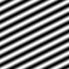
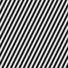
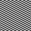
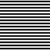
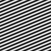
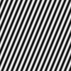
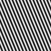
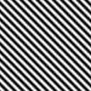
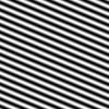
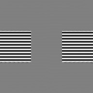
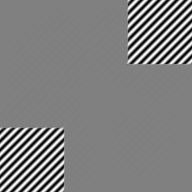
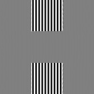
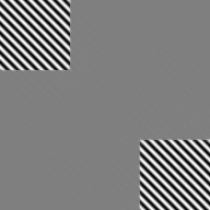
Here, C1,C2subscript𝐶1subscript𝐶2C_{1},C_{2}\in\mathbb{R} are constants, ωd𝜔superscript𝑑\omega\in\mathbb{R}^{d}, ω0𝜔0\omega\neq 0 is a direction vector and \cdot represents the standard inner product of vectors in dsuperscript𝑑\mathbb{R}^{d}. Figure 1 shows a visualization of these oscillatory functions (7) in Ω2Ωsuperscript2\Omega\subset\mathbb{R}^{2} with different values of ω1subscript𝜔1\omega_{1} and ω2subscript𝜔2\omega_{2}. Our goal is to find a differential equation that is, in some sense, compatible with the second-order TGV functional according to [12] and such that the functions u𝑢u according (7) are exactly the solutions for all C1,C2subscript𝐶1subscript𝐶2C_{1},C_{2}\in\mathbb{R}. For this purpose, consider the equation

u+𝐜u=0,𝑢𝐜𝑢0\mathcal{E}\nabla u+\mathbf{c}u=0, (8)

where 𝐜=ωω𝐜tensor-product𝜔𝜔\mathbf{c}=\omega\otimes\omega is the tensor (or outer) product, i.e., cij=ωiωjsubscript𝑐𝑖𝑗subscript𝜔𝑖subscript𝜔𝑗c_{ij}=\omega_{i}\omega_{j}, i,j=1,,dformulae-sequence𝑖𝑗1𝑑i,j=1,\ldots,d. Indeed, this equation already possesses the desired properties.

Refer to caption
Refer to caption
Refer to caption
Refer to caption
Refer to caption
Refer to caption
Figure 1: Visualization of sinusoidal oscillations on Ω2Ωsuperscript2\Omega\subset\mathbb{R}^{2} according to (7). (a) ω1=0,ω2=0.5formulae-sequencesubscript𝜔10subscript𝜔20.5\omega_{1}=0,\omega_{2}=0.5; (b) ω1=0.5,ω2=0formulae-sequencesubscript𝜔10.5subscript𝜔20\omega_{1}=0.5,\omega_{2}=0; (c) ω1=0.25,ω2=0.5formulae-sequencesubscript𝜔10.25subscript𝜔20.5\omega_{1}=0.25,\omega_{2}=0.5; (d) ω1=0.5,ω2=0.25formulae-sequencesubscript𝜔10.5subscript𝜔20.25\omega_{1}=0.5,\omega_{2}=0.25; (e) ω1=1,ω2=0.5formulae-sequencesubscript𝜔11subscript𝜔20.5\omega_{1}=1,\omega_{2}=0.5; (f) ω1=0.5,ω2=1formulae-sequencesubscript𝜔10.5subscript𝜔21\omega_{1}=0.5,\omega_{2}=1.
Lemma 1.

Let 𝐜=ωω𝐜tensor-product𝜔𝜔\mathbf{c}=\omega\otimes\omega with ωd𝜔superscript𝑑\omega\in\mathbb{R}^{d}, ω0𝜔0\omega\neq 0. Then, a function uC2(Ω)𝑢superscript𝐶2Ωu\in C^{2}(\Omega) solves (8) if and only if u𝑢u has a representation (7) for some C1,C2subscript𝐶1subscript𝐶2C_{1},C_{2}\in\mathbb{R}.

Proof.

Note that it suffices to prove the statement locally, i.e., without loss of generality, ΩΩ\Omega is an open hypercube in dsuperscript𝑑\mathbb{R}^{d} of the form Ω=]a1,b1[××]ad,bd[\Omega={]{a_{1},b_{1}}[}\times\cdots\times{]{a_{d},b_{d}}[}.

Clearly, ()ij=2xixjsubscript𝑖𝑗superscript2subscript𝑥𝑖subscript𝑥𝑗(\mathcal{E}\nabla)_{ij}=\frac{\partial^{2}}{\partial x_{i}\partial x_{j}} and 2xixjsin(ωx)=ωiωjsin(ωx)superscript2subscript𝑥𝑖subscript𝑥𝑗𝜔𝑥subscript𝜔𝑖subscript𝜔𝑗𝜔𝑥\frac{\partial^{2}}{\partial x_{i}\partial x_{j}}\sin(\omega\cdot x)=-\omega_{i}\omega_{j}\sin(\omega\cdot x) as well as 2xixjcos(ωx)=ωiωjcos(ωx)superscript2subscript𝑥𝑖subscript𝑥𝑗𝜔𝑥subscript𝜔𝑖subscript𝜔𝑗𝜔𝑥\frac{\partial^{2}}{\partial x_{i}\partial x_{j}}\cos(\omega\cdot x)=-\omega_{i}\omega_{j}\cos(\omega\cdot x). Thus, if uC2(Ω)𝑢superscript𝐶2Ωu\in C^{2}(\Omega) has the representation (7), then (8) follows.

For the converse direction, we proceed inductively with respect to the dimension d𝑑d. Starting with d=1𝑑1d=1, equation (8) reads as 2ux12u+ω12u=0superscript2𝑢superscriptsubscript𝑥12𝑢superscriptsubscript𝜔12𝑢0\frac{\partial^{2}u}{\partial x_{1}^{2}}u+\omega_{1}^{2}u=0 where ω10subscript𝜔10\omega_{1}\neq 0 which is an ordinary differential equation with solutions of the form (7). Next, fix d1𝑑1d\geq 1 and suppose that (8) implies (7) for some C1,C2subscript𝐶1subscript𝐶2C_{1},C_{2}\in\mathbb{R} whenever uC2(Ω)𝑢superscript𝐶2Ωu\in C^{2}(\Omega) for ΩdΩsuperscript𝑑\Omega\subset\mathbb{R}^{d} an open hypercube. Let ωd+1𝜔superscript𝑑1\omega\in\mathbb{R}^{d+1} such that ω0𝜔0\omega\neq 0. After a possible interchange of axes, we can assume, without loss of generality, that (ω1,,ωd)0subscript𝜔1subscript𝜔𝑑0(\omega_{1},\ldots,\omega_{d})\neq 0. Let Ωd+1Ωsuperscript𝑑1\Omega\subset\mathbb{R}^{d+1} be an open hypercube and uC2(Ω)𝑢superscript𝐶2Ωu\in C^{2}(\Omega) satisfy (8) (in dimension d+1𝑑1d+1). Then, in particular, 2uxixj+ωiωju=0superscript2𝑢subscript𝑥𝑖subscript𝑥𝑗subscript𝜔𝑖subscript𝜔𝑗𝑢0\frac{\partial^{2}u}{\partial x_{i}\partial x_{j}}+\omega_{i}\omega_{j}u=0 for i,j=1,,dformulae-sequence𝑖𝑗1𝑑i,j=1,\ldots,d. Denoting by xsuperscript𝑥x^{\prime} the projection of a vector xd+1𝑥superscript𝑑1x\in\mathbb{R}^{d+1} onto the first d𝑑d components, i.e., x=(x1,,xd)superscript𝑥subscript𝑥1subscript𝑥𝑑x^{\prime}=(x_{1},\ldots,x_{d}), the induction hypothesis gives

u(x)=C1(xd+1)sin(ωx)+C2(xd+1)cos(ωx)forxΩ.formulae-sequence𝑢𝑥subscript𝐶1subscript𝑥𝑑1superscript𝜔superscript𝑥subscript𝐶2subscript𝑥𝑑1superscript𝜔superscript𝑥for𝑥Ωu(x)=C_{1}(x_{d+1})\sin(\omega^{\prime}\cdot x^{\prime})+C_{2}(x_{d+1})\cos(\omega^{\prime}\cdot x^{\prime})\quad\text{for}\quad x\in\Omega.

As xωxmaps-to𝑥superscript𝜔superscript𝑥x\mapsto\omega^{\prime}\cdot x^{\prime} is non-constant, we are able to choose x,x¯Ω𝑥¯𝑥Ωx,\bar{x}\in\Omega such that the matrix

[sin(ωx)cos(ωx)sin(ωx¯)cos(ωx¯)]matrixsuperscript𝜔superscript𝑥superscript𝜔superscript𝑥superscript𝜔superscript¯𝑥superscript𝜔superscript¯𝑥\begin{bmatrix}\sin(\omega^{\prime}\cdot x^{\prime})&\cos(\omega^{\prime}\cdot x^{\prime})\\ \sin(\omega^{\prime}\cdot\bar{x}^{\prime})&\cos(\omega^{\prime}\cdot\bar{x}^{\prime})\end{bmatrix}

has full rank. Using that 2uxd+12+ωd+12u=0superscript2𝑢superscriptsubscript𝑥𝑑12superscriptsubscript𝜔𝑑12𝑢0\frac{\partial^{2}u}{\partial x_{d+1}^{2}}+\omega_{d+1}^{2}u=0 in neighborhoods of x𝑥x and x¯¯𝑥\bar{x} consequently yields that there are constants C1,1,C1,2,C2,1,C2,2subscript𝐶11subscript𝐶12subscript𝐶21subscript𝐶22C_{1,1},C_{1,2},C_{2,1},C_{2,2} such that

Ck(xd+1)={Ck,1xd+1+Ck,2ifωd+1=0,Ck,1sin(ωd+1xd+1)+Ck,2cos(ωd+1xd+1)otherwise,subscript𝐶𝑘subscript𝑥𝑑1casessubscript𝐶𝑘1subscript𝑥𝑑1subscript𝐶𝑘2ifsubscript𝜔𝑑10subscript𝐶𝑘1subscript𝜔𝑑1subscript𝑥𝑑1subscript𝐶𝑘2subscript𝜔𝑑1subscript𝑥𝑑1otherwiseC_{k}(x_{d+1})=\begin{cases}C_{k,1}x_{d+1}+C_{k,2}&\text{if}\ \omega_{d+1}=0,\\ C_{k,1}\sin(\omega_{d+1}x_{d+1})+C_{k,2}\cos(\omega_{d+1}x_{d+1})&\text{otherwise},\end{cases}\quad

for k=1,2𝑘12k=1,2. If ωd+1=0subscript𝜔𝑑10\omega_{d+1}=0, then 2uxixd+1+ωiωd+1u=0superscript2𝑢subscript𝑥𝑖subscript𝑥𝑑1subscript𝜔𝑖subscript𝜔𝑑1𝑢0\frac{\partial^{2}u}{\partial x_{i}\partial x_{d+1}}+\omega_{i}\omega_{d+1}u=0 for i{1,,d}𝑖1𝑑i\in\{1,\ldots,d\} such that ωi0subscript𝜔𝑖0\omega_{i}\neq 0 gives that C1,1cos(ωx)C2,1sin(ωx)=0subscript𝐶11superscript𝜔superscript𝑥subscript𝐶21superscript𝜔superscript𝑥0C_{1,1}\cos(\omega^{\prime}\cdot x^{\prime})-C_{2,1}\sin(\omega^{\prime}\cdot x^{\prime})=0 for xΩ𝑥Ωx\in\Omega. Consequently, C1,1=C2,1=0subscript𝐶11subscript𝐶210C_{1,1}=C_{2,1}=0 and the induction step is complete.

In the case ωd+10subscript𝜔𝑑10\omega_{d+1}\neq 0, 2uxixd+1+ωiωd+1u=0superscript2𝑢subscript𝑥𝑖subscript𝑥𝑑1subscript𝜔𝑖subscript𝜔𝑑1𝑢0\frac{\partial^{2}u}{\partial x_{i}\partial x_{d+1}}+\omega_{i}\omega_{d+1}u=0 for i{1,,d}𝑖1𝑑i\in\{1,\ldots,d\} such that ωi0subscript𝜔𝑖0\omega_{i}\neq 0 implies

u(x)𝑢𝑥\displaystyle u(x) =(C1,2sin(ωd+1xd+1)C1,1cos(ωd+1xd+1))cos(ωx)absentsubscript𝐶12subscript𝜔𝑑1subscript𝑥𝑑1subscript𝐶11subscript𝜔𝑑1subscript𝑥𝑑1superscript𝜔superscript𝑥\displaystyle=\bigl{(}C_{1,2}\sin(\omega_{d+1}x_{d+1})-C_{1,1}\cos(\omega_{d+1}x_{d+1})\bigr{)}\cos(\omega^{\prime}\cdot x^{\prime})
+(C2,1cos(ωd+1xd+1)C2,2sin(ωd+1xd+1))sin(ωx)subscript𝐶21subscript𝜔𝑑1subscript𝑥𝑑1subscript𝐶22subscript𝜔𝑑1subscript𝑥𝑑1superscript𝜔superscript𝑥\displaystyle\quad+\bigl{(}C_{2,1}\cos(\omega_{d+1}x_{d+1})-C_{2,2}\sin(\omega_{d+1}x_{d+1})\bigr{)}\sin(\omega^{\prime}\cdot x^{\prime})

for xΩ𝑥Ωx\in\Omega. Comparing coefficients yields C2,2=C1,1subscript𝐶22subscript𝐶11C_{2,2}=-C_{1,1} as well as C2,1=C1,2subscript𝐶21subscript𝐶12C_{2,1}=C_{1,2}. Plugging this into the representation of u𝑢u gives, by virtue of the angle sum identities for sine and cosine,

u(x)=C2,1sin(ωx+ωd+1xd+1)+C2,2cos(ωx+ωd+1xd+1)=C2,1sin(ωx)+C2,2cos(ωx)𝑢𝑥subscript𝐶21superscript𝜔superscript𝑥subscript𝜔𝑑1subscript𝑥𝑑1subscript𝐶22superscript𝜔superscript𝑥subscript𝜔𝑑1subscript𝑥𝑑1subscript𝐶21𝜔𝑥subscript𝐶22𝜔𝑥u(x)=C_{2,1}\sin(\omega^{\prime}\cdot x^{\prime}+\omega_{d+1}x_{d+1})+C_{2,2}\cos(\omega^{\prime}\cdot x^{\prime}+\omega_{d+1}x_{d+1})=C_{2,1}\sin(\omega\cdot x)+C_{2,2}\cos(\omega\cdot x)

for xΩ𝑥Ωx\in\Omega, proving the induction step for ωd+10subscript𝜔𝑑10\omega_{d+1}\neq 0. ∎

Based on this observation, we aim at designing a functional that is suitable to measure piecewise oscillatory functions u𝑢u with direction ω0𝜔0\omega\neq 0, i.e.,

u=i=1nχΩi(x)ui(x),withχΩi(x)={1,if xΩi,0,otherwise,formulae-sequence𝑢superscriptsubscript𝑖1𝑛subscript𝜒subscriptΩ𝑖𝑥subscript𝑢𝑖𝑥withsubscript𝜒subscriptΩ𝑖𝑥cases1if xΩi0otherwiseu=\sum_{i=1}^{n}\chi_{\Omega_{i}}(x)u_{i}(x),\quad\text{with}\quad\chi_{\Omega_{i}}(x)=\begin{cases}1,&\text{if $x\in\Omega_{i}$},\\ 0,&\text{otherwise},\end{cases}

where Ω1Ωn=ΩsubscriptΩ1subscriptΩ𝑛Ω\Omega_{1}\cup\ldots\cup\Omega_{n}=\Omega, ΩiΩj=subscriptΩ𝑖subscriptΩ𝑗\Omega_{i}\cap\Omega_{j}=\emptyset, ijfor-all𝑖𝑗\forall i\neq j and ui(x)=C1,icos(ωx)+C2,isin(ωx)subscript𝑢𝑖𝑥subscript𝐶1𝑖𝜔𝑥subscript𝐶2𝑖𝜔𝑥u_{i}(x)=C_{1,i}\cos(\omega\cdot x)+C_{2,i}\sin(\omega\cdot x), for some C1,i,C2,isubscript𝐶1𝑖subscript𝐶2𝑖C_{1,i},C_{2,i}\in\mathbb{R}, i=1,,n𝑖1𝑛i=1,\ldots,n.

Let us now motivate the definition of oscillation TGV. It is easily seen that the kernel of second-order TGV according to (5) can be obtained by solving uw=0𝑢𝑤0\nabla u-w=0 and w=0𝑤0\mathcal{E}w=0 for uBV(Ω),wBD(Ω)formulae-sequence𝑢BVΩ𝑤BDΩu\in\operatorname{BV}(\Omega),w\in\operatorname{BD}(\Omega). This leads to all u𝑢u for which u=0𝑢0\mathcal{E}\nabla u=0 holds in the distributional sense which can be shown to be exactly the affine functions. Based on this and the fact that oscillatory functions are solving (8), we see in turn that this class can be represented by uw=0𝑢𝑤0\nabla u-w=0 and w+𝐜u=0𝑤𝐜𝑢0\mathcal{E}w+\mathbf{c}u=0 for uBV(Ω),wBD(Ω)formulae-sequence𝑢BVΩ𝑤BDΩu\in\operatorname{BV}(\Omega),w\in\operatorname{BD}(\Omega). This leads to the following generalization of second-order TGV we call oscillation TGV.

Definition 1.

Let α,β>0𝛼𝛽0\alpha,\beta>0 and 𝐜=ωω𝐜tensor-product𝜔𝜔\mathbf{c}=\omega\otimes\omega where ωd𝜔superscript𝑑\omega\in\mathbb{R}^{d}. For uL1(Ω)𝑢superscript𝐿1Ωu\in L^{1}(\Omega), the oscillation TGV functional is defined as follows:

TGVα,β,𝐜osci(u)=minwBD(Ω)αuw+βw+𝐜usubscriptsuperscriptTGVosci𝛼𝛽𝐜𝑢subscript𝑤BDΩ𝛼subscriptnorm𝑢𝑤𝛽subscriptnorm𝑤𝐜𝑢\operatorname{TGV}^{\operatorname{osci}}_{\alpha,\beta,\mathbf{c}}(u)=\min_{w\in\operatorname{BD}(\Omega)}\alpha\|\nabla u-w\|_{\mathcal{M}}+\beta\|\mathcal{E}w+\mathbf{c}u\|_{\mathcal{M}} (9)

if uBV(Ω)𝑢BVΩu\in\operatorname{BV}(\Omega) and TGVα,β,𝐜osci(u)=subscriptsuperscriptTGVosci𝛼𝛽𝐜𝑢\operatorname{TGV}^{\operatorname{osci}}_{\alpha,\beta,\mathbf{c}}(u)=\infty if uL1(Ω)BV(Ω)𝑢superscript𝐿1ΩBVΩu\in L^{1}(\Omega)\setminus\operatorname{BV}(\Omega).

The usage of the minimum will be justified later. Note that for ω=0𝜔0\omega=0, the definition reduces to the well-known second-order TGV with weights α,β𝛼𝛽\alpha,\beta, i.e., we have TGVα,β,𝐜osci(u)=TGVα,β2(u)subscriptsuperscriptTGVosci𝛼𝛽𝐜𝑢superscriptsubscriptTGV𝛼𝛽2𝑢\operatorname{TGV}^{\operatorname{osci}}_{\alpha,\beta,\mathbf{c}}(u)=\operatorname{TGV}_{\alpha,\beta}^{2}(u) if ω=0𝜔0\omega=0. One can easily see that oscillation TGV is proper and convex; we focus on showing its lower semi-continuity in Lpsuperscript𝐿𝑝L^{p}-spaces along with some basic properties in the following.

2.2 Basic properties

For the purpose of establishing lower semi-continuity, we need some tools and notions from convex analysis, see, for instance, [45, 5], for an overview. For a functional F:X],]F:X\rightarrow{]{-\infty,\infty}]}, the effective domain is defined as domF={xX:F(x)<}dom𝐹conditional-set𝑥𝑋𝐹𝑥\operatorname{dom}F=\{x\in X:F(x)<\infty\}, and F𝐹F is called proper if domFdom𝐹\operatorname{dom}F\neq\emptyset. The indicator functional is defined as

K(x)={0if xK,+otherwise.subscript𝐾𝑥cases0if xKotherwise\mathcal{I}_{K}(x)=\begin{cases}0&\text{if $x\in K$},\\ +\infty&\text{otherwise}.\\ \end{cases}

As usual, we also denote by ,\langle\cdot,\cdot\rangle the duality product of Xsuperscript𝑋X^{\ast} and X𝑋X between the Banach spaces Xsuperscript𝑋X^{\ast} and X𝑋X. Moreover, recall that the convex conjugate functional for a proper F:X],]F:X\to{]{-\infty,\infty}]} is given by F:X],]F^{\ast}:X^{\ast}\to{]{-\infty,\infty}]} with F(x)=supxXx,xF(x)superscript𝐹superscript𝑥subscriptsupremum𝑥𝑋superscript𝑥𝑥𝐹𝑥F^{\ast}(x^{\ast})=\sup\limits_{x\in X}\ \langle x^{\ast},x\rangle-F(x). With these prerequisites, we give a predual formulation of oscillation TGV which will then imply lower semi-continuity and in particular justify the minimum in the definition (9).

Proposition 1.

Fix α,β>0𝛼𝛽0\alpha,\beta>0 and 𝐜=ωω𝐜tensor-product𝜔𝜔\mathbf{c}=\omega\otimes\omega, ωd𝜔superscript𝑑\omega\in\mathbb{R}^{d}. For each uL1(Ω)𝑢superscript𝐿1Ωu\in L^{1}(\Omega), we have

TGVα,β,𝐜osci(u)=sup{Ωu(div2ϕ+𝐜ϕ)dx:ϕCc(Ω,Sd×d),ϕβ,divϕα},subscriptsuperscriptTGVosci𝛼𝛽𝐜𝑢supremumconditional-setsubscriptΩ𝑢superscriptdiv2italic-ϕ𝐜italic-ϕdifferential-d𝑥formulae-sequenceitalic-ϕsuperscriptsubscript𝐶𝑐Ωsuperscript𝑆𝑑𝑑formulae-sequencesubscriptnormitalic-ϕ𝛽subscriptnormdivitalic-ϕ𝛼\operatorname{TGV}^{\operatorname{osci}}_{\alpha,\beta,\mathbf{c}}(u)=\sup\left\{\int_{\Omega}u(\operatorname{div}^{2}\phi+\mathbf{c}\cdot\phi)\,\mathrm{d}{x}:\phi\in C_{c}^{\infty}(\Omega,S^{d\times d}),\|\phi\|_{\infty}\leq\beta,\|\operatorname{div}\phi\|_{\infty}\leq\alpha\right\}, (10)

where 𝐜ϕ𝐜italic-ϕ\mathbf{c}\cdot\phi denotes the pointwise Frobenius inner product of 𝐜𝐜\mathbf{c} and the symmetric matrix field ϕitalic-ϕ\phi. Moreover, the minimum in the definition of TGVα,β,𝐜osci(u)subscriptsuperscriptTGVosci𝛼𝛽𝐜𝑢\operatorname{TGV}^{\operatorname{osci}}_{\alpha,\beta,\mathbf{c}}(u) according to (9) is obtained.

Proof.

Firstly observing that Cc(Ω,Sd×d)superscriptsubscript𝐶𝑐Ωsuperscript𝑆𝑑𝑑C_{c}^{\infty}(\Omega,S^{d\times d}) is dense in the Banach space C02(Ω,Sd×d)superscriptsubscript𝐶02Ωsuperscript𝑆𝑑𝑑C_{0}^{2}(\Omega,S^{d\times d}) with respect to the C2superscript𝐶2C^{2} norm given by ϕC2=max(ϕ,ϕ,2ϕ)subscriptnormitalic-ϕsuperscript𝐶2subscriptnormitalic-ϕsubscriptnormitalic-ϕsubscriptnormsuperscript2italic-ϕ\|{\phi}\|_{C^{2}}=\max\ (\|{\phi}\|_{\infty},\|{\nabla\phi}\|_{\infty},\|{\nabla^{2}\phi}\|_{\infty}), we can replace Cc(Ω,Sd×d)superscriptsubscript𝐶𝑐Ωsuperscript𝑆𝑑𝑑C_{c}^{\infty}(\Omega,S^{d\times d}) in (10) by C02(Ω,Sd×d)superscriptsubscript𝐶02Ωsuperscript𝑆𝑑𝑑C_{0}^{2}(\Omega,S^{d\times d}): Indeed, for ϕC02(Ω,Sd×d)italic-ϕsuperscriptsubscript𝐶02Ωsuperscript𝑆𝑑𝑑\phi\in C_{0}^{2}(\Omega,S^{d\times d}) such that ϕβsubscriptnormitalic-ϕ𝛽\|{\phi}\|_{\infty}\leq\beta and divϕαsubscriptnormdivitalic-ϕ𝛼\|{\operatorname{div}\phi}\|_{\infty}\leq\alpha one may choose a sequence {ϕn}superscriptitalic-ϕ𝑛\{\phi^{n}\} in Cc2(Ω,Sd×d)superscriptsubscript𝐶𝑐2Ωsuperscript𝑆𝑑𝑑C_{c}^{2}(\Omega,S^{d\times d}) such that limnϕn=ϕsubscript𝑛superscriptitalic-ϕ𝑛italic-ϕ\lim_{n\to\infty}\phi^{n}=\phi in C02(Ω,Sd×d)superscriptsubscript𝐶02Ωsuperscript𝑆𝑑𝑑C_{0}^{2}(\Omega,S^{d\times d}). Convolving with smooth mollifiers, we can moreover ensure that, without loss of generality, each ϕnCc(Ω,Sd×d)superscriptitalic-ϕ𝑛superscriptsubscript𝐶𝑐Ωsuperscript𝑆𝑑𝑑\phi^{n}\in C_{c}^{\infty}(\Omega,S^{d\times d}). Now, letting λn=max(ϕn/β,divϕn/α,1)subscript𝜆𝑛subscriptnormsuperscriptitalic-ϕ𝑛𝛽subscriptnormdivsuperscriptitalic-ϕ𝑛𝛼1\lambda_{n}=\max\ (\|{\phi^{n}}\|_{\infty}/\beta,\|{\operatorname{div}\phi^{n}}\|_{\infty}/\alpha,1) we see by continuous embedding C02(Ω,Sd×d)C0(Ω,Sd×d)superscriptsubscript𝐶02Ωsuperscript𝑆𝑑𝑑subscript𝐶0Ωsuperscript𝑆𝑑𝑑C_{0}^{2}(\Omega,S^{d\times d})\hookrightarrow C_{0}(\Omega,S^{d\times d}) as well as continuity of div:C02(Ω,Sd×d)C0(Ω,d):divsuperscriptsubscript𝐶02Ωsuperscript𝑆𝑑𝑑subscript𝐶0Ωsuperscript𝑑\operatorname{div}:C_{0}^{2}(\Omega,S^{d\times d})\to C_{0}(\Omega,\mathbb{R}^{d}) that limnλn=1subscript𝑛subscript𝜆𝑛1\lim_{n\to\infty}\lambda_{n}=1. Thus, limnλn1ϕn=ϕsubscript𝑛superscriptsubscript𝜆𝑛1superscriptitalic-ϕ𝑛italic-ϕ\lim_{n\to\infty}\lambda_{n}^{-1}\phi^{n}=\phi and for each n𝑛n, we have λn1ϕnβsubscriptnormsuperscriptsubscript𝜆𝑛1superscriptitalic-ϕ𝑛𝛽\|{\lambda_{n}^{-1}\phi^{n}}\|_{\infty}\leq\beta as well as divλn1ϕnαsubscriptnormdivsuperscriptsubscript𝜆𝑛1superscriptitalic-ϕ𝑛𝛼\|{\operatorname{div}\lambda_{n}^{-1}\phi^{n}}\|_{\infty}\leq\alpha. This proves the density.

Choosing X=C02(Ω,Sd×d)𝑋superscriptsubscript𝐶02Ωsuperscript𝑆𝑑𝑑X=C_{0}^{2}(\Omega,S^{d\times d}), Y=C01(Ω,d)𝑌superscriptsubscript𝐶01Ωsuperscript𝑑Y=C_{0}^{1}(\Omega,\mathbb{R}^{d}) with norm ηC1=max(η,η)subscriptnorm𝜂superscript𝐶1subscriptnorm𝜂subscriptnorm𝜂\|{\eta}\|_{C^{1}}=\max\ (\|{\eta}\|_{\infty},\|{\nabla\eta}\|_{\infty}), Λ=div(X,Y)Λdiv𝑋𝑌\Lambda=\operatorname{div}\in\mathcal{L}(X,Y), and defining

F1subscript𝐹1\displaystyle F_{1} :X],],\displaystyle:X\rightarrow{]{-\infty,\infty}]}, F1(ϕ)subscript𝐹1italic-ϕ\displaystyle F_{1}(\phi) ={β}(ϕ)𝐜u,ϕ,\displaystyle=\mathcal{I}_{\{\|\cdot\|_{\infty}\leq\beta\}}(\phi)-\langle\mathbf{c}u,\phi\rangle,
F2subscript𝐹2\displaystyle F_{2} :Y],],\displaystyle:Y\rightarrow{]{-\infty,\infty}]}, F2(η)subscript𝐹2𝜂\displaystyle F_{2}(\eta) ={α}(η)u,divη,\displaystyle=\mathcal{I}_{\{\|\cdot\|_{\infty}\leq\alpha\}}(\eta)-\langle u,\operatorname{div}\eta\rangle,

where ,\langle{\cdot},{\cdot}\rangle is the L1superscript𝐿1L^{1}Lsuperscript𝐿L^{\infty} duality pairing, we can equivalently write the supremum in (10) as

infϕXF1(ϕ)+F2(Λϕ).subscriptinfimumitalic-ϕ𝑋subscript𝐹1italic-ϕsubscript𝐹2Λitalic-ϕ-\inf_{\phi\in X}F_{1}(\phi)+F_{2}(\Lambda\phi).

According to [3], the Fenchel–Rockafellar duality formula is valid if

Y=λ0λ(domF2ΛdomF1).𝑌subscript𝜆0𝜆domsubscript𝐹2Λdomsubscript𝐹1Y=\bigcup_{\lambda\geq 0}\lambda(\operatorname{dom}F_{2}-\Lambda\operatorname{dom}F_{1}).

This is indeed true since for each ηY𝜂𝑌\eta\in Y, we can write η=λ(λ1ηdiv0)𝜂𝜆superscript𝜆1𝜂div0\eta=\lambda(\lambda^{-1}\eta-\operatorname{div}0) with λ1ηαsubscriptnormsuperscript𝜆1𝜂𝛼\|\lambda^{-1}\eta\|_{\infty}\leq\alpha and 0domF10domsubscript𝐹10\in\operatorname{dom}F_{1}. Thus, there is no duality gap between the primal and the dual problems and the dual problem admits a solution, i.e.,

(infϕXF1(ϕ)+F2(Λϕ))+(minwYF1(Λw)+F2(w))=0.subscriptinfimumitalic-ϕ𝑋subscript𝐹1italic-ϕsubscript𝐹2Λitalic-ϕsubscript𝑤superscript𝑌superscriptsubscript𝐹1superscriptΛ𝑤superscriptsubscript𝐹2𝑤0\Bigl{(}\inf_{\phi\in X}F_{1}(\phi)+F_{2}(\Lambda\phi)\Bigr{)}+\Bigl{(}\min_{w\in Y^{\ast}}F_{1}^{\ast}(-\Lambda^{\ast}w)+F_{2}^{\ast}(w)\Bigr{)}=0.

(In the case the primal functional is unbounded from below, this equation has to be understood in the sense that the dual functional is constant \infty.) Now, we calculate the convex conjugates on the right-hand side. For, a distribution wY=C01(Ω,d)𝑤superscript𝑌superscriptsubscript𝐶01superscriptΩsuperscript𝑑w\in Y^{\ast}=C_{0}^{1}(\Omega,\mathbb{R}^{d})^{\ast} we have that Λw=divw=wsuperscriptΛ𝑤superscriptdiv𝑤𝑤-\Lambda^{*}w=-\operatorname{div}^{*}w=\mathcal{E}w in the distributional sense: Indeed, testing divwsuperscriptdiv𝑤-\operatorname{div}^{*}w with ϕCc(Ω,Sd×d)italic-ϕsuperscriptsubscript𝐶𝑐Ωsuperscript𝑆𝑑𝑑\phi\in C_{c}^{\infty}(\Omega,S^{d\times d}) gives divw,ϕ=w,divϕ=w,ϕsuperscriptdiv𝑤italic-ϕ𝑤divitalic-ϕ𝑤italic-ϕ\langle{-\operatorname{div}^{*}w},{\phi}\rangle=\langle{w},{-\operatorname{div}\phi}\rangle=\langle{\mathcal{E}w},{\phi}\rangle for the duality pairing ,\langle{\cdot},{\cdot}\rangle of distributions and test functions. Thus,

F1(Λw)=supϕX,ϕβw,divϕ+𝐜u,ϕ=supϕCc(Ω,Sd×d),ϕβw,ϕ+𝐜u,ϕ=βw+𝐜uF_{1}^{\ast}(-\Lambda^{\ast}w)=\sup_{\scriptstyle\phi\in X,\atop\scriptstyle\|\phi\|_{\infty}\leq\beta}\langle w,-\operatorname{div}\phi\rangle+\langle\mathbf{c}u,\phi\rangle=\sup_{\begin{subarray}{c}\phi\in C_{c}^{\infty}(\Omega,S^{d\times d}),\\ \|{\phi}\|_{\infty}\leq\beta\end{subarray}}\langle\mathcal{E}w,\phi\rangle+\langle\mathbf{c}u,\phi\rangle=\beta\|\mathcal{E}w+\mathbf{c}u\|_{\mathcal{M}}

where, by definition of the Radon norm for distributions, w+𝐜u=subscriptnorm𝑤𝐜𝑢\|{\mathcal{E}w+\mathbf{c}u}\|_{\mathcal{M}}=\infty if w+𝐜u𝑤𝐜𝑢\mathcal{E}w+\mathbf{c}u is not in (Ω,Sd×d)Ωsuperscript𝑆𝑑𝑑\mathcal{M}(\Omega,S^{d\times d}). Note that for the above identity, we used that {ϕCc(Ω,Sd×d):ϕβ}conditional-setitalic-ϕsuperscriptsubscript𝐶𝑐Ωsuperscript𝑆𝑑𝑑subscriptnormitalic-ϕ𝛽\{\phi\in C_{c}^{\infty}(\Omega,S^{d\times d}):\|{\phi}\|_{\infty}\leq\beta\} is dense in {ϕC02(Ω,Sd×d):ϕβ}conditional-setitalic-ϕsuperscriptsubscript𝐶02Ωsuperscript𝑆𝑑𝑑subscriptnormitalic-ϕ𝛽\{\phi\in C_{0}^{2}(\Omega,S^{d\times d}):\|{\phi}\|_{\infty}\leq\beta\} which can be seen analogously to the density argument at the beginning of the proof. Now, since uL1(Ω)𝑢superscript𝐿1Ωu\in L^{1}(\Omega), we have 𝐜uL1(Ω,Sd×d)𝐜𝑢superscript𝐿1Ωsuperscript𝑆𝑑𝑑\mathbf{c}u\in L^{1}(\Omega,S^{d\times d}) and w+𝐜usubscriptnorm𝑤𝐜𝑢\|{\mathcal{E}w+\mathbf{c}u}\|_{\mathcal{M}} is finite if and only if w(Ω,Sd×d)𝑤Ωsuperscript𝑆𝑑𝑑\mathcal{E}w\in\mathcal{M}(\Omega,S^{d\times d}). But this is the case if and only if wBD(Ω)𝑤BDΩw\in\operatorname{BD}(\Omega).

Furthermore, we see that div=superscriptdiv\operatorname{div}^{\ast}=-\nabla in the distributional sense, so by arguments analogous to the above, it follows that

F2(w)=supηY,ηαw,η+u,divη=αuwF_{2}^{\ast}(w)=\sup_{\scriptstyle\eta\in Y,\atop\scriptstyle\|\eta\|_{\infty}\leq\alpha}\langle w,\eta\rangle+\langle u,\operatorname{div}\eta\rangle=\alpha\|\nabla u-w\|_{\mathcal{M}}

where, again, uw=subscriptnorm𝑢𝑤\|{\nabla u-w}\|_{\mathcal{M}}=\infty if uw(Ω,d)𝑢𝑤Ωsuperscript𝑑\nabla u-w\notin\mathcal{M}(\Omega,\mathbb{R}^{d}). Consequently, for wBD(Ω)𝑤BDΩw\in\operatorname{BD}(\Omega), the norm is finite if and only if uBV(Ω)𝑢BVΩu\in\operatorname{BV}(\Omega).

These considerations yield that indeed, minimizing F1(Λw)+F2(w)superscriptsubscript𝐹1superscriptΛ𝑤superscriptsubscript𝐹2𝑤F_{1}^{\ast}(-\Lambda^{\ast}w)+F_{2}^{\ast}(w) is equivalent to minimizing the functional in (9), that it suffices to choose w𝑤w from BD(Ω)BDΩ\operatorname{BD}(\Omega) instead of Ysuperscript𝑌Y^{*}, and that the minimum is \infty if and only if uBV(Ω)𝑢BVΩu\notin\operatorname{BV}(\Omega). This gives the desired identity (10).

In particular, as the optimal value for the dual problem is attained, there always exists a wBD(Ω)𝑤BDΩw\in\operatorname{BD}(\Omega) which admits the minimum in (9). ∎

Since the dual formulation of oscillation TGV is a pointwise supremum of continuous functions, we can easily derive that it is lower semi-continuous with respect to the Lpsuperscript𝐿𝑝L^{p}-topology for each p[1,]𝑝1p\in[1,\infty]. In summary, it is a semi-norm that shares the following properties:

Proposition 2.

The functional TGVα,β,𝐜oscisubscriptsuperscriptTGVosci𝛼𝛽𝐜\operatorname{TGV}^{\operatorname{osci}}_{\alpha,\beta,\mathbf{c}} is a proper, and lower semi-continuous one-homogeneous functional on L1(Ω)superscript𝐿1ΩL^{1}(\Omega) that satisfies the triangle inequality. Further, TGVα,β,𝐜osci(u)=0subscriptsuperscriptTGVosci𝛼𝛽𝐜𝑢0\operatorname{TGV}^{\operatorname{osci}}_{\alpha,\beta,\mathbf{c}}(u)=0 if and only if u𝑢u satisfies (7) for some C1,C2subscript𝐶1subscript𝐶2C_{1},C_{2}\in\mathbb{R} in case of ω0𝜔0\omega\neq 0 and u𝑢u affine in case of ω=0𝜔0\omega=0.

Proof.

We only discuss the case ω0𝜔0\omega\neq 0 as, by the above remark, TGVα,β,𝐜oscisubscriptsuperscriptTGVosci𝛼𝛽𝐜\operatorname{TGV}^{\operatorname{osci}}_{\alpha,\beta,\mathbf{c}} reduces to second-order TGV in case ω=0𝜔0\omega=0 for which the claimed properties were established in [12].

By Proposition 1, TGVα,β,𝐜oscisubscriptsuperscriptTGVosci𝛼𝛽𝐜\operatorname{TGV}^{\operatorname{osci}}_{\alpha,\beta,\mathbf{c}} is the convex conjugate of a convex indicator functional associated with a nonempty, convex and balanced set. Thus, it is proper, convex and positive one-homogeneous; we refer to the proof of statement 1 of Proposition 3.3 in [12]. In particular, TGVα,β,𝐜oscisubscriptsuperscriptTGVosci𝛼𝛽𝐜\operatorname{TGV}^{\operatorname{osci}}_{\alpha,\beta,\mathbf{c}} satisfies the triangle inequality. Further, for each ϕCc(Ω,Sd×d)italic-ϕsuperscriptsubscript𝐶𝑐Ωsuperscript𝑆𝑑𝑑\phi\in C_{c}^{\infty}(\Omega,S^{d\times d}), the mapping uΩu(div2ϕ+𝐜ϕ)dxmaps-to𝑢subscriptΩ𝑢superscriptdiv2italic-ϕ𝐜italic-ϕdifferential-d𝑥u\mapsto\int_{\Omega}u(\operatorname{div}^{2}\phi+\mathbf{c}\cdot\phi)\,\mathrm{d}{x} is linear and continuous on L1(Ω)superscript𝐿1ΩL^{1}(\Omega), so TGVα,β,𝐜oscisubscriptsuperscriptTGVosci𝛼𝛽𝐜\operatorname{TGV}^{\operatorname{osci}}_{\alpha,\beta,\mathbf{c}} is lower semi-continuous on L1(Ω)superscript𝐿1ΩL^{1}(\Omega) as the pointwise supremum of continuous functionals, see (10).

Finally, for uL1(Ω)𝑢superscript𝐿1Ωu\in L^{1}(\Omega), we have TGVα,β,𝐜osci(u)=0subscriptsuperscriptTGVosci𝛼𝛽𝐜𝑢0\operatorname{TGV}^{\operatorname{osci}}_{\alpha,\beta,\mathbf{c}}(u)=0 if and only if Ωu(div2ϕ+𝐜ϕ)dx=0subscriptΩ𝑢superscriptdiv2italic-ϕ𝐜italic-ϕdifferential-d𝑥0\int_{\Omega}u(\operatorname{div}^{2}\phi+\mathbf{c}\cdot\phi)\,\mathrm{d}{x}=0 for all ϕCc(Ω,Sd×d)italic-ϕsuperscriptsubscript𝐶𝑐Ωsuperscript𝑆𝑑𝑑\phi\in C_{c}^{\infty}(\Omega,S^{d\times d}) with ϕβsubscriptnormitalic-ϕ𝛽\|{\phi}\|_{\infty}\leq\beta, divϕαsubscriptnormdivitalic-ϕ𝛼\|{\operatorname{div}\phi}\|_{\infty}\leq\alpha. The latter, however, is equivalent to Ωu(div2ϕ+𝐜ϕ)dx=0subscriptΩ𝑢superscriptdiv2italic-ϕ𝐜italic-ϕdifferential-d𝑥0\int_{\Omega}u(\operatorname{div}^{2}\phi+\mathbf{c}\cdot\phi)\,\mathrm{d}{x}=0 for all ϕCc2(Ω,Sd×d)italic-ϕsuperscriptsubscript𝐶𝑐2Ωsuperscript𝑆𝑑𝑑\phi\in C_{c}^{2}(\Omega,S^{d\times d}) which, in turn, means u+𝐜u=0𝑢𝐜𝑢0\mathcal{E}\nabla u+\mathbf{c}u=0 in ΩΩ\Omega in the weak sense.

We show that this equation is also satisfied in the strong sense. For this purpose, observe that it is in particular true for uρϵ𝑢subscript𝜌italic-ϵu\ast\rho_{\epsilon} with a mollifier ρϵCc(Bϵ(0))subscript𝜌italic-ϵsuperscriptsubscript𝐶𝑐subscript𝐵italic-ϵ0\rho_{\epsilon}\in C_{c}^{\infty}(B_{\epsilon}(0)) and each subdomain ΩΩsuperscriptΩΩ\Omega^{\prime}\subset\Omega with dist(Ω,Ω)>ϵdistsuperscriptΩΩitalic-ϵ\operatorname{dist}(\Omega^{\prime},\partial\Omega)>\epsilon. Indeed, this follows from

Ω(uρϵ)(div2ϕ+𝐜ϕ)dx=Ωu(div2(ϕρ¯ϵ)+𝐜(ϕρ¯ϵ))dx=0subscriptsuperscriptΩ𝑢subscript𝜌italic-ϵsuperscriptdiv2italic-ϕ𝐜italic-ϕdifferential-d𝑥subscriptΩ𝑢superscriptdiv2italic-ϕsubscript¯𝜌italic-ϵ𝐜italic-ϕsubscript¯𝜌italic-ϵdifferential-d𝑥0\int_{\Omega^{\prime}}(u\ast\rho_{\epsilon})(\operatorname{div}^{2}\phi+\mathbf{c}\cdot\phi)\,\mathrm{d}{x}=\int_{\Omega}u\bigl{(}\operatorname{div}^{2}(\phi\ast\bar{\rho}_{\epsilon})+\mathbf{c}\cdot(\phi\ast\bar{\rho}_{\epsilon})\bigr{)}\,\mathrm{d}{x}=0

where ρ¯ϵ(x)=ρϵ(x)subscript¯𝜌italic-ϵ𝑥subscript𝜌italic-ϵ𝑥\bar{\rho}_{\epsilon}(x)=\rho_{\epsilon}(-x), since ϕρ¯ϵCc(Ω,Sd×d)italic-ϕsubscript¯𝜌italic-ϵsuperscriptsubscript𝐶𝑐Ωsuperscript𝑆𝑑𝑑\phi\ast\bar{\rho}_{\epsilon}\in C_{c}^{\infty}(\Omega,S^{d\times d}) whenever ϕCc(Ω,Sd×d)italic-ϕsuperscriptsubscript𝐶𝑐superscriptΩsuperscript𝑆𝑑𝑑\phi\in C_{c}^{\infty}(\Omega^{\prime},S^{d\times d}). But uρϵCc(Ω)𝑢subscript𝜌italic-ϵsubscriptsuperscript𝐶𝑐superscriptΩu\ast\rho_{\epsilon}\in C^{\infty}_{c}(\Omega^{\prime}), so we have (uρϵ)+𝐜(uρϵ)=0𝑢subscript𝜌italic-ϵ𝐜𝑢subscript𝜌italic-ϵ0\mathcal{E}\nabla(u\ast\rho_{\epsilon})+\mathbf{c}(u\ast\rho_{\epsilon})=0 in ΩsuperscriptΩ\Omega^{\prime} also in the strong sense. Thus, uρϵ𝑢subscript𝜌italic-ϵu\ast\rho_{\epsilon} satisfies (7) in ΩsuperscriptΩ\Omega^{\prime}. Fixing ΩsuperscriptΩ\Omega^{\prime} and letting ϵ0italic-ϵ0\epsilon\to 0 now gives uρϵu𝑢subscript𝜌italic-ϵ𝑢u\ast\rho_{\epsilon}\to u in L1(Ω)superscript𝐿1superscriptΩL^{1}(\Omega^{\prime}). In particular, uρϵ𝑢subscript𝜌italic-ϵu\ast\rho_{\epsilon} converges to u𝑢u in the finite-dimensional space of functions in L1(Ω)superscript𝐿1superscriptΩL^{1}(\Omega^{\prime}) satisfying (7), which implies by closedness of finite-dimensional spaces that u𝑢u also satisfies (7) for some C1,C2subscript𝐶1subscript𝐶2C_{1},C_{2}\in\mathbb{R} and, consequently, uC2(Ω)𝑢superscript𝐶2superscriptΩu\in C^{2}(\Omega^{\prime}). As ΩsuperscriptΩ\Omega^{\prime} can be chosen arbitrarily such that Ω¯¯superscriptΩ\overline{\Omega^{\prime}} is compact in ΩΩ\Omega, the latter also holds true in ΩΩ\Omega. ∎

Furthermore, TGVα,β,𝐜oscisubscriptsuperscriptTGVosci𝛼𝛽𝐜\operatorname{TGV}^{\operatorname{osci}}_{\alpha,\beta,\mathbf{c}} is translation invariant as well as rotationally invariant with respect to a rotated 𝐜𝐜\mathbf{c}:

Proposition 3.

For each yd𝑦superscript𝑑y\in\mathbb{R}^{d} and uL1(Ω)𝑢superscript𝐿1Ωu\in L^{1}(\Omega), if u~(x)=u(xy)~𝑢𝑥𝑢𝑥𝑦\tilde{u}(x)=u(x-y), then TGVα,β,𝐜osci(u~)=TGVα,β,𝐜osci(u)subscriptsuperscriptTGVosci𝛼𝛽𝐜~𝑢subscriptsuperscriptTGVosci𝛼𝛽𝐜𝑢\operatorname{TGV}^{\operatorname{osci}}_{\alpha,\beta,\mathbf{c}}(\tilde{u})=\operatorname{TGV}^{\operatorname{osci}}_{\alpha,\beta,\mathbf{c}}(u), i.e., TGVα,β,𝐜oscisubscriptsuperscriptTGVosci𝛼𝛽𝐜\operatorname{TGV}^{\operatorname{osci}}_{\alpha,\beta,\mathbf{c}} is translation-invariant.

Furthermore, for each orthonormal matrix Od×d𝑂superscript𝑑𝑑O\in\mathbb{R}^{d\times d} and uL1(Ω)𝑢superscript𝐿1Ωu\in L^{1}(\Omega), if u~(x)=u(Ox)~𝑢𝑥𝑢𝑂𝑥\tilde{u}(x)=u(Ox), then TGVα,β,𝐜osci(u~)=TGVα,β,𝐜~osci(u)subscriptsuperscriptTGVosci𝛼𝛽𝐜~𝑢subscriptsuperscriptTGVosci𝛼𝛽~𝐜𝑢\operatorname{TGV}^{\operatorname{osci}}_{\alpha,\beta,\mathbf{c}}(\tilde{u})=\operatorname{TGV}^{\operatorname{osci}}_{\alpha,\beta,\tilde{\mathbf{c}}}(u) with 𝐜~=OωOω~𝐜tensor-product𝑂𝜔𝑂𝜔\tilde{\mathbf{c}}=O\omega\otimes O\omega. In other words, TGVα,β,𝐜oscisubscriptsuperscriptTGVosci𝛼𝛽𝐜{\rm TGV}^{\operatorname{osci}}_{\alpha,\beta,\mathbf{c}} is rotationally invariant.

Proof.

First, let us define the following set

Kα,β(Ω)={ϕCc(Ω,Sd×d):ϕβ,divϕα}.subscript𝐾𝛼𝛽Ωconditional-setitalic-ϕsuperscriptsubscript𝐶𝑐Ωsuperscript𝑆𝑑𝑑formulae-sequencesubscriptnormitalic-ϕ𝛽subscriptnormdivitalic-ϕ𝛼K_{\alpha,\beta}(\Omega)=\left\{\phi\in C_{c}^{\infty}(\Omega,S^{d\times d}):\|\phi\|_{\infty}\leq\beta,\ \|\operatorname{div}\phi\|_{\infty}\leq\alpha\right\}.

For ϕKα,β(Ω+y)italic-ϕsubscript𝐾𝛼𝛽Ω𝑦\phi\in K_{\alpha,\beta}(\Omega+y) we set ϕ~(x)=ϕ(x+y)~italic-ϕ𝑥italic-ϕ𝑥𝑦\tilde{\phi}(x)=\phi(x+y). Then, ϕ~βsubscriptnorm~italic-ϕ𝛽\|{\tilde{\phi}}\|_{\infty}\leq\beta, divϕ~(x)=divϕ(x+y)div~italic-ϕ𝑥divitalic-ϕ𝑥𝑦\operatorname{div}\tilde{\phi}(x)=\operatorname{div}\phi(x+y) and div2ϕ~(x)=div2ϕ(x+y)superscriptdiv2~italic-ϕ𝑥superscriptdiv2italic-ϕ𝑥𝑦\operatorname{div}^{2}\tilde{\phi}(x)=\operatorname{div}^{2}\phi(x+y) such that divϕ~αsubscriptnormdiv~italic-ϕ𝛼\|{\operatorname{div}\tilde{\phi}}\|_{\infty}\leq\alpha and, consequently, ϕ~Kα,β(Ω)~italic-ϕsubscript𝐾𝛼𝛽Ω\tilde{\phi}\in K_{\alpha,\beta}(\Omega). Interchanging the roles of ϕitalic-ϕ\phi and ϕ~~italic-ϕ\tilde{\phi}, it follows that ϕKα,β(Ω+y)italic-ϕsubscript𝐾𝛼𝛽Ω𝑦\phi\in K_{\alpha,\beta}(\Omega+y) if and only if ϕ~Kα,β(Ω)~italic-ϕsubscript𝐾𝛼𝛽Ω\tilde{\phi}\in K_{\alpha,\beta}(\Omega). For ϕKα,β(Ω+y)italic-ϕsubscript𝐾𝛼𝛽Ω𝑦\phi\in K_{\alpha,\beta}(\Omega+y) it holds that

Ω+yu~(x)(div2ϕ(x)+𝐜ϕ(x))dx=Ωu(x)(div2ϕ~(x)+𝐜ϕ~(x))dx,subscriptΩ𝑦~𝑢𝑥superscriptdiv2italic-ϕ𝑥𝐜italic-ϕ𝑥differential-d𝑥subscriptΩ𝑢𝑥superscriptdiv2~italic-ϕ𝑥𝐜~italic-ϕ𝑥differential-d𝑥\int_{\Omega+y}\tilde{u}(x)\bigl{(}\operatorname{div}^{2}\phi(x)+\mathbf{c}\cdot\phi(x)\bigr{)}\,\mathrm{d}{x}=\int_{\Omega}u(x)\bigl{(}\operatorname{div}^{2}\tilde{\phi}(x)+\mathbf{c}\cdot\tilde{\phi}(x)\bigr{)}\,\mathrm{d}{x},

hence taking the supremum yields with the above that TGVα,β,𝐜osci(u~)=TGVα,β,𝐜osci(u)superscriptsubscriptTGV𝛼𝛽𝐜osci~𝑢superscriptsubscriptTGV𝛼𝛽𝐜osci𝑢\operatorname{TGV}_{\alpha,\beta,\mathbf{c}}^{\operatorname{osci}}(\tilde{u})=\operatorname{TGV}_{\alpha,\beta,\mathbf{c}}^{\operatorname{osci}}(u).

For ϕKα,β(OTΩ)italic-ϕsubscript𝐾𝛼𝛽superscript𝑂𝑇Ω\phi\in K_{\alpha,\beta}(O^{T}\Omega) we set ϕ~(x)=Oϕ(OTx)OT~italic-ϕ𝑥𝑂italic-ϕsuperscript𝑂𝑇𝑥superscript𝑂𝑇\tilde{\phi}(x)=O\phi(O^{T}x)O^{T} which satisfies ϕ~Cc2(Ω,Sd×d)~italic-ϕsuperscriptsubscript𝐶𝑐2Ωsuperscript𝑆𝑑𝑑\tilde{\phi}\in C_{c}^{2}(\Omega,S^{d\times d}) as well as ϕ~βsubscriptnorm~italic-ϕ𝛽\|{\tilde{\phi}}\|_{\infty}\leq\beta, the latter due to the invariance of the Frobenius norm under orthonormal similarity transforms. Moreover, we have

divϕ~(x)=divϕ(OTx)OT,div2ϕ~(x)=div2ϕ(OTx),formulae-sequencediv~italic-ϕ𝑥divitalic-ϕsuperscript𝑂𝑇𝑥superscript𝑂𝑇superscriptdiv2~italic-ϕ𝑥superscriptdiv2italic-ϕsuperscript𝑂𝑇𝑥\operatorname{div}\tilde{\phi}(x)=\operatorname{div}\phi(O^{T}x)O^{T},\qquad\operatorname{div}^{2}\tilde{\phi}(x)=\operatorname{div}^{2}\phi(O^{T}x),

see, for instance, (A.4) in [12]. Therefore, divϕ~αsubscriptnormdiv~italic-ϕ𝛼\|{\operatorname{div}\tilde{\phi}}\|_{\infty}\leq\alpha, so ϕ~Kα,β(Ω)~italic-ϕsubscript𝐾𝛼𝛽Ω\tilde{\phi}\in K_{\alpha,\beta}(\Omega). Interchanging the roles of ϕitalic-ϕ\phi and ϕ~~italic-ϕ\tilde{\phi} it follows that ϕKα,β(OTΩ)italic-ϕsubscript𝐾𝛼𝛽superscript𝑂𝑇Ω\phi\in K_{\alpha,\beta}(O^{T}\Omega) if and only if ϕ~Kα,β(Ω)~italic-ϕsubscript𝐾𝛼𝛽Ω\tilde{\phi}\in K_{\alpha,\beta}(\Omega).

Eventually, for each ϕKα,β(OTΩ)italic-ϕsubscript𝐾𝛼𝛽superscript𝑂𝑇Ω\phi\in K_{\alpha,\beta}(O^{T}\Omega), we have

OTΩu~(x)(div2ϕ(x)+𝐜ϕ(x))dxsubscriptsuperscript𝑂𝑇Ω~𝑢𝑥superscriptdiv2italic-ϕ𝑥𝐜italic-ϕ𝑥differential-d𝑥\displaystyle\int_{O^{T}\Omega}\tilde{u}(x)\bigl{(}\operatorname{div}^{2}\phi(x)+\mathbf{c}\cdot\phi(x)\bigr{)}\,\mathrm{d}{x} =OTΩu(Ox)(div2ϕ(x)+𝐜ϕ(x))dxabsentsubscriptsuperscript𝑂𝑇Ω𝑢𝑂𝑥superscriptdiv2italic-ϕ𝑥𝐜italic-ϕ𝑥differential-d𝑥\displaystyle=\int_{O^{T}\Omega}u(Ox)\bigl{(}\operatorname{div}^{2}\phi(x)+\mathbf{c}\cdot\phi(x)\bigr{)}\,\mathrm{d}{x}
=Ωu(x)(div2ϕ(OTx)+𝐜ϕ(OTx))dxabsentsubscriptΩ𝑢𝑥superscriptdiv2italic-ϕsuperscript𝑂𝑇𝑥𝐜italic-ϕsuperscript𝑂𝑇𝑥differential-d𝑥\displaystyle=\int_{\Omega}u(x)\bigl{(}\operatorname{div}^{2}\phi(O^{T}x)+\mathbf{c}\cdot\phi(O^{T}x)\bigr{)}\,\mathrm{d}{x}
=Ωu(x)(div2ϕ~(x)+𝐜(OTϕ~(x)O))dxabsentsubscriptΩ𝑢𝑥superscriptdiv2~italic-ϕ𝑥𝐜superscript𝑂𝑇~italic-ϕ𝑥𝑂differential-d𝑥\displaystyle=\int_{\Omega}u(x)\bigl{(}\operatorname{div}^{2}\tilde{\phi}(x)+\mathbf{c}\cdot(O^{T}\tilde{\phi}(x)O)\bigr{)}\,\mathrm{d}{x}
=Ωu(x)(div2ϕ~(x)+(O𝐜OT)ϕ~(x))dx.absentsubscriptΩ𝑢𝑥superscriptdiv2~italic-ϕ𝑥𝑂𝐜superscript𝑂𝑇~italic-ϕ𝑥differential-d𝑥\displaystyle=\int_{\Omega}u(x)\bigl{(}\operatorname{div}^{2}\tilde{\phi}(x)+(O\mathbf{c}O^{T})\cdot\tilde{\phi}(x)\bigr{)}\,\mathrm{d}{x}.

Taking the supremum and noting that O𝐜OT=OωOω=𝐜~𝑂𝐜superscript𝑂𝑇tensor-product𝑂𝜔𝑂𝜔~𝐜O\mathbf{c}O^{T}=O\omega\otimes O\omega=\tilde{\mathbf{c}} then leads to TGVα,β,𝐜osci(u~)=TGVα,β,𝐜~osci(u)subscriptsuperscriptTGVosci𝛼𝛽𝐜~𝑢subscriptsuperscriptTGVosci𝛼𝛽~𝐜𝑢\operatorname{TGV}^{\operatorname{osci}}_{\alpha,\beta,\mathbf{c}}(\tilde{u})=\operatorname{TGV}^{\operatorname{osci}}_{\alpha,\beta,\tilde{\mathbf{c}}}(u). ∎

We would like to examine Banach spaces that are associated with the semi-norm TGVα,β,𝐜oscisubscriptsuperscriptTGVosci𝛼𝛽𝐜\operatorname{TGV}^{\operatorname{osci}}_{\alpha,\beta,\mathbf{c}}. To construct a norm, we add, as it is also done in case of TGVTGV\operatorname{TGV}, the L1superscript𝐿1L^{1}-norm. The resulting Banach space

BGVosci(Ω)={uL1(Ω):TGVα,β,𝐜osci(u)<},uBGVosci=u1+TGVα,β,𝐜osci(u)formulae-sequencesuperscriptBGVosciΩconditional-set𝑢superscript𝐿1ΩsubscriptsuperscriptTGVosci𝛼𝛽𝐜𝑢subscriptnorm𝑢superscriptBGVoscisubscriptnorm𝑢1subscriptsuperscriptTGVosci𝛼𝛽𝐜𝑢\operatorname{BGV}^{\operatorname{osci}}(\Omega)=\{u\in L^{1}(\Omega):\operatorname{TGV}^{\operatorname{osci}}_{\alpha,\beta,\mathbf{c}}(u)<\infty\},\qquad\|{u}\|_{\operatorname{BGV}^{\operatorname{osci}}}=\|{u}\|_{1}+\operatorname{TGV}^{\operatorname{osci}}_{\alpha,\beta,\mathbf{c}}(u)

then coincides with BV(Ω)BVΩ\operatorname{BV}(\Omega). Indeed, this is a consequence of the equivalence of norms which is proven in the following lemma.

Lemma 2.

For each ωd𝜔superscript𝑑\omega\in\mathbb{R}^{d}, there exist constants 0<c<C<0𝑐𝐶0<c<C<\infty such that for each uL1(Ω)𝑢superscript𝐿1Ωu\in L^{1}(\Omega), we have

cuBVu1+TGVα,β,𝐜osci(u)CuBV.𝑐subscriptnorm𝑢BVsubscriptnorm𝑢1subscriptsuperscriptTGVosci𝛼𝛽𝐜𝑢𝐶subscriptnorm𝑢BVc\|u\|_{\operatorname{BV}}\leq\|u\|_{1}+\operatorname{TGV}^{\operatorname{osci}}_{\alpha,\beta,\mathbf{c}}(u)\leq C\|u\|_{\operatorname{BV}}. (11)
Proof.

Setting w=0𝑤0w=0 in the definition (9) implies immediately that

TGVα,β,𝐜osci(u)αu+β𝐜u1αTV(u)+β|ω|2u1.subscriptsuperscriptTGVosci𝛼𝛽𝐜𝑢𝛼subscriptnorm𝑢𝛽subscriptnorm𝐜𝑢1𝛼TV𝑢𝛽superscript𝜔2subscriptnorm𝑢1\operatorname{TGV}^{\operatorname{osci}}_{\alpha,\beta,\mathbf{c}}(u)\leq\alpha\|\nabla u\|_{\mathcal{M}}+\beta\|\mathbf{c}u\|_{1}\leq\alpha\operatorname{TV}(u)+\beta|{\omega}|^{2}\|{u}\|_{1}.

Adding the L1superscript𝐿1L^{1}-norm on both sides give the second inequality of (11) for C=max{α,1+β|ω|2}𝐶𝛼1𝛽superscript𝜔2C=\max\{\alpha,1+\beta|{\omega}|^{2}\}.

For the converse inequality, we may assume uBV(Ω)𝑢BVΩu\in\operatorname{BV}(\Omega) since otherwise, TGVα,β,𝐜osci(u)=subscriptsuperscriptTGVosci𝛼𝛽𝐜𝑢\operatorname{TGV}^{\operatorname{osci}}_{\alpha,\beta,\mathbf{c}}(u)=\infty by definition. Due to the norm equivalence in BV(Ω)BVΩ\operatorname{BV}(\Omega) and BGVα,β2(Ω)subscriptsuperscriptBGV2𝛼𝛽Ω\operatorname{BGV}^{2}_{\alpha,\beta}(\Omega) shown, e.g., in [51, 14, 11], there exists a constant C1>0subscript𝐶10C_{1}>0 such that for each wBD(Ω)𝑤BDΩw\in\operatorname{BD}(\Omega),

C1uBVu1+TGVα,β2(u)u1+αuw+βw=u1+αuw+β||w+𝐜u𝐜uu1+αuw+βw+𝐜u+β𝐜u1C2(u1+αuw+βw+𝐜u)\begin{split}C_{1}\|u\|_{\operatorname{BV}}&\leq\|u\|_{1}+\operatorname{TGV}^{2}_{\alpha,\beta}(u)\\ &\leq\|u\|_{1}+\alpha\|\nabla u-w\|_{\mathcal{M}}+\beta\|\mathcal{E}w\|_{\mathcal{M}}\\ &=\|u\|_{1}+\alpha\|\nabla u-w\|_{\mathcal{M}}+\beta||\mathcal{E}w+\mathbf{c}u-\mathbf{c}u\|_{\mathcal{M}}\\ &\leq\|u\|_{1}+\alpha\|\nabla u-w\|_{\mathcal{M}}+\beta\|\mathcal{E}w+\mathbf{c}u\|_{\mathcal{M}}+\beta\|\mathbf{c}u\|_{1}\\ &\leq C_{2}(\|u\|_{1}+\alpha\|\nabla u-w\|_{\mathcal{M}}+\beta\|\mathcal{E}w+\mathbf{c}u\|_{\mathcal{M}})\end{split}

where C2=max{1,1+β|ω|2}subscript𝐶211𝛽superscript𝜔2C_{2}=\max\{1,1+\beta|{\omega}|^{2}\}. Choosing c=C1C2𝑐subscript𝐶1subscript𝐶2c=\frac{C_{1}}{C_{2}} and minimizing over wBD(Ω)𝑤BDΩw\in\operatorname{BD}(\Omega) finally yields the first inequality of (11). ∎

Depending on the results of Lemma 2, we can further deduce following inequality of Poincaré–Wirtinger type which implies the coercivity of oscillation TGV in the BVBV\operatorname{BV}-space.

Proposition 4.

Let P:L1(Ω)ker(TGVα,β,𝐜osci):𝑃superscript𝐿1ΩkernelsubscriptsuperscriptTGVosci𝛼𝛽𝐜P:L^{1}(\Omega)\rightarrow\ker(\operatorname{TGV}^{\operatorname{osci}}_{\alpha,\beta,\mathbf{c}}) a linear and continuous projection onto the kernel ker(TGVα,β,𝐜osci)kernelsubscriptsuperscriptTGVosci𝛼𝛽𝐜\ker(\operatorname{TGV}^{\operatorname{osci}}_{\alpha,\beta,\mathbf{c}}) (which exists), then there is a C>0𝐶0C>0 such that

uPuBVCTGVα,β,𝐜osci(u)for alluBV(Ω).formulae-sequencesubscriptnorm𝑢𝑃𝑢BV𝐶subscriptsuperscriptTGVosci𝛼𝛽𝐜𝑢for all𝑢BVΩ\|u-Pu\|_{\operatorname{BV}}\leq C\operatorname{TGV}^{\operatorname{osci}}_{\alpha,\beta,\mathbf{c}}(u)\quad\text{for all}\quad u\in\operatorname{BV}(\Omega). (12)
Proof.

If the statement is not true, then there exists a sequence {un}superscript𝑢𝑛\{u^{n}\} in BV(Ω)BVΩ\operatorname{BV}(\Omega) such that

unPunBV=1,TGVα,β,𝐜osci(un)1n,formulae-sequencesubscriptnormsuperscript𝑢𝑛𝑃superscript𝑢𝑛BV1subscriptsuperscriptTGVosci𝛼𝛽𝐜superscript𝑢𝑛1𝑛\|u^{n}-Pu^{n}\|_{\operatorname{BV}}=1,\quad\operatorname{TGV}^{\operatorname{osci}}_{\alpha,\beta,\mathbf{c}}(u^{n})\leq\frac{1}{n},

for all n𝑛n\in\mathbb{N}. By the compact embedding BV(Ω)L1(Ω)BVΩsuperscript𝐿1Ω\operatorname{BV}(\Omega)\hookrightarrow L^{1}(\Omega), it follows that limnunPun=usubscript𝑛superscript𝑢𝑛𝑃superscript𝑢𝑛superscript𝑢\lim\limits_{n\rightarrow\infty}u^{n}-Pu^{n}=u^{\ast} in L1(Ω)superscript𝐿1ΩL^{1}(\Omega) for some subsequence (not relabeled). We have P(unPun)=0𝑃superscript𝑢𝑛𝑃superscript𝑢𝑛0P(u^{n}-Pu^{n})=0 for all n𝑛n, consequently, the limit has to satisfy Pu=0𝑃superscript𝑢0Pu^{\ast}=0 by continuity of P𝑃P in L1(Ω)superscript𝐿1ΩL^{1}(\Omega).

As P𝑃P projects onto the kernel of TGVα,β,𝐜oscisubscriptsuperscriptTGVosci𝛼𝛽𝐜\operatorname{TGV}^{\operatorname{osci}}_{\alpha,\beta,\mathbf{c}}, we have TGVα,β,𝐜osci(Pun)=0subscriptsuperscriptTGVosci𝛼𝛽𝐜𝑃superscript𝑢𝑛0\operatorname{TGV}^{\operatorname{osci}}_{\alpha,\beta,\mathbf{c}}(Pu^{n})=0 for all n𝑛n and can deduce that TGVα,β,𝐜osci(unPun)=TGVα,β,𝐜osci(un)subscriptsuperscriptTGVosci𝛼𝛽𝐜superscript𝑢𝑛𝑃superscript𝑢𝑛subscriptsuperscriptTGVosci𝛼𝛽𝐜superscript𝑢𝑛\operatorname{TGV}^{\operatorname{osci}}_{\alpha,\beta,\mathbf{c}}(u^{n}-Pu^{n})=\operatorname{TGV}^{\operatorname{osci}}_{\alpha,\beta,\mathbf{c}}(u^{n}). On the other hand, the lower semi-continuity of TGVα,β,𝐜oscisubscriptsuperscriptTGVosci𝛼𝛽𝐜\operatorname{TGV}^{\operatorname{osci}}_{\alpha,\beta,\mathbf{c}} implies

TGVα,β,𝐜osci(u)lim infnTGVα,β,𝐜osci(un)=0,subscriptsuperscriptTGVosci𝛼𝛽𝐜superscript𝑢subscriptlimit-infimum𝑛subscriptsuperscriptTGVosci𝛼𝛽𝐜superscript𝑢𝑛0\operatorname{TGV}^{\operatorname{osci}}_{\alpha,\beta,\mathbf{c}}(u^{\ast})\leq\liminf_{n\rightarrow\infty}\operatorname{TGV}^{\operatorname{osci}}_{\alpha,\beta,\mathbf{c}}(u^{n})=0,

hence uker(TGVα,β,𝐜osci)ker(P)superscript𝑢kernelsubscriptsuperscriptTGVosci𝛼𝛽𝐜kernel𝑃u^{\ast}\in\ker(\operatorname{TGV}^{\operatorname{osci}}_{\alpha,\beta,\mathbf{c}})\cap\ker(P). As P𝑃P is a projection with ran(P)=ker(TGVα,β,𝐜osci)ran𝑃kernelsubscriptsuperscriptTGVosci𝛼𝛽𝐜\operatorname{ran}(P)=\ker(\operatorname{TGV}^{\operatorname{osci}}_{\alpha,\beta,\mathbf{c}}), this implies u=Pu=0superscript𝑢𝑃superscript𝑢0u^{*}=Pu^{*}=0, so limnunPun=0subscript𝑛superscript𝑢𝑛𝑃superscript𝑢𝑛0\lim\limits_{n\rightarrow\infty}u^{n}-Pu^{n}=0 in L1(Ω)superscript𝐿1ΩL^{1}(\Omega).

Now, according to Lemma 2, there is a C1>0subscript𝐶10C_{1}>0 such that

unPunBVC1(unPun1+TGVα,β,𝐜osci(un)),subscriptnormsuperscript𝑢𝑛𝑃superscript𝑢𝑛BVsubscript𝐶1subscriptnormsuperscript𝑢𝑛𝑃superscript𝑢𝑛1subscriptsuperscriptTGVosci𝛼𝛽𝐜superscript𝑢𝑛\|u^{n}-Pu^{n}\|_{\operatorname{BV}}\leq C_{1}\bigl{(}\|u^{n}-Pu^{n}\|_{1}+\operatorname{TGV}^{\operatorname{osci}}_{\alpha,\beta,\mathbf{c}}(u^{n})\bigr{)}, (13)

so limnunPun=0subscript𝑛superscript𝑢𝑛𝑃superscript𝑢𝑛0\lim\limits_{n\rightarrow\infty}u^{n}-Pu^{n}=0 in BV(Ω)BVΩ\operatorname{BV}(\Omega) which is a contradiction to unPunBV=1subscriptnormsuperscript𝑢𝑛𝑃superscript𝑢𝑛BV1\|u^{n}-Pu^{n}\|_{\operatorname{BV}}=1 for all n𝑛n. ∎

Remark 1.

By continuous embedding BV(Ω)Lp(Ω)BVΩsuperscript𝐿𝑝Ω\operatorname{BV}(\Omega)\hookrightarrow L^{p}(\Omega) for 1pd/(d1)1𝑝𝑑𝑑11\leq p\leq d/(d-1) we have in particular coercivity of TGVα,β,𝐜oscisubscriptsuperscriptTGVosci𝛼𝛽𝐜\operatorname{TGV}^{\operatorname{osci}}_{\alpha,\beta,\mathbf{c}} in Lp(Ω)superscript𝐿𝑝ΩL^{p}(\Omega) according to

uPupCTGVα,β,𝐜osci(u)for eachuLp(Ω).formulae-sequencesubscriptnorm𝑢𝑃𝑢𝑝𝐶subscriptsuperscriptTGVosci𝛼𝛽𝐜𝑢for each𝑢superscript𝐿𝑝Ω\|{u-Pu}\|_{p}\leq C\operatorname{TGV}^{\operatorname{osci}}_{\alpha,\beta,\mathbf{c}}(u)\quad\text{for each}\quad u\in L^{p}(\Omega).

3 Infimal convolution of oscillation TGV functionals

So far, we examined oscillation TGV functionals associated with a single direction ωd𝜔superscript𝑑\omega\in\mathbb{R}^{d}. Next, we aim at incorporating multiple directions ω1,,ωmdsubscript𝜔1subscript𝜔𝑚superscript𝑑\omega_{1},\ldots,\omega_{m}\in\mathbb{R}^{d} into one functional in order to represent structured oscillations in an image with respect to multiple orientations and frequencies. This will be done in terms of the infimal convolution. Recall that, given two functionals J1subscript𝐽1J_{1} and J2subscript𝐽2J_{2}, their infimal convolution is defined by

(J1J2)(u)=infvJ1(uv)+J2(v)=infu=u1+u2J1(u1)+J2(u2).subscript𝐽1subscript𝐽2𝑢subscriptinfimum𝑣subscript𝐽1𝑢𝑣subscript𝐽2𝑣subscriptinfimum𝑢subscript𝑢1subscript𝑢2subscript𝐽1subscript𝑢1subscript𝐽2subscript𝑢2(J_{1}\hskip 0.83328pt\Box\hskip 0.83328ptJ_{2})(u)=\inf_{v}J_{1}(u-v)+J_{2}(v)=\inf_{u=u_{1}+u_{2}}J_{1}(u_{1})+J_{2}(u_{2}). (14)

For m𝑚m functionals J1,,Jmsubscript𝐽1subscript𝐽𝑚J_{1},\ldots,J_{m} the definition is iterated leading to

(J1Jm)(u)=infu=u1++umi=1mJi(ui).subscript𝐽1subscript𝐽𝑚𝑢subscriptinfimum𝑢subscript𝑢1subscript𝑢𝑚superscriptsubscript𝑖1𝑚subscript𝐽𝑖subscript𝑢𝑖(J_{1}\hskip 0.83328pt\Box\hskip 0.83328pt\ldots\hskip 0.83328pt\Box\hskip 0.83328ptJ_{m})(u)=\inf_{u=u_{1}+\ldots+u_{m}}\sum_{i=1}^{m}J_{i}(u_{i}).

We aim at studying the m𝑚m-fold infimal convolution of oscillation TGV given as follows:

ICTGVα,β,𝐜osci(u)=(TGVα1,β1,𝐜1osciTGVαm,βm,𝐜mosci)(u)=infu=u1++umi=1mTGVαi,βi,𝐜iosci(ui).subscriptsuperscriptICTGVosci𝛼𝛽𝐜𝑢subscriptsuperscriptTGVoscisubscript𝛼1subscript𝛽1subscript𝐜1subscriptsuperscriptTGVoscisubscript𝛼𝑚subscript𝛽𝑚subscript𝐜𝑚𝑢subscriptinfimum𝑢subscript𝑢1subscript𝑢𝑚superscriptsubscript𝑖1𝑚subscriptsuperscriptTGVoscisubscript𝛼𝑖subscript𝛽𝑖subscript𝐜𝑖subscript𝑢𝑖\operatorname{ICTGV}^{\operatorname{osci}}_{\vec{\alpha},\vec{\beta},\vec{\mathbf{c}}}(u)=(\operatorname{TGV}^{\operatorname{osci}}_{\alpha_{1},\beta_{1},\mathbf{c}_{1}}\hskip 0.83328pt\Box\hskip 0.83328pt\ldots\hskip 0.83328pt\Box\hskip 0.83328pt\operatorname{TGV}^{\operatorname{osci}}_{\alpha_{m},\beta_{m},\mathbf{c}_{m}})(u)=\inf_{u=u_{1}+\ldots+u_{m}}\sum_{i=1}^{m}\operatorname{TGV}^{\operatorname{osci}}_{\alpha_{i},\beta_{i},\mathbf{c}_{i}}(u_{i}). (15)

Here, α=(α1,,αm)𝛼subscript𝛼1subscript𝛼𝑚\vec{\alpha}=(\alpha_{1},\ldots,\alpha_{m}), β=(β1,,βm)𝛽subscript𝛽1subscript𝛽𝑚\vec{\beta}=(\beta_{1},\ldots,\beta_{m}) are vectors of positive weights and 𝐜=(𝐜1,,𝐜m)𝐜subscript𝐜1subscript𝐜𝑚\vec{\mathbf{c}}=(\mathbf{c}_{1},\ldots,\mathbf{c}_{m}) is given by 𝐜i=ωiωisubscript𝐜𝑖tensor-productsubscript𝜔𝑖subscript𝜔𝑖\mathbf{c}_{i}=\omega_{i}\otimes\omega_{i} for ω1,,ωmdsubscript𝜔1subscript𝜔𝑚superscript𝑑\omega_{1},\ldots,\omega_{m}\in\mathbb{R}^{d}.

It is well-known that the infimal convolution of the convex functionals is also convex. Also, since TGVαi,βi,𝐜iosci(0)=0subscriptsuperscriptTGVoscisubscript𝛼𝑖subscript𝛽𝑖subscript𝐜𝑖00\operatorname{TGV}^{\operatorname{osci}}_{\alpha_{i},\beta_{i},\mathbf{c}_{i}}(0)=0 for each i𝑖i, one can easily obtain that ICTGVα,β,𝐜oscisubscriptsuperscriptICTGVosci𝛼𝛽𝐜\operatorname{ICTGV}^{\operatorname{osci}}_{\vec{\alpha},\vec{\beta},\vec{\mathbf{c}}} is proper. Therefore, in the following section, we concentrate on the coercivity and lower semi-continuity of ICTGVα,β,𝐜oscisubscriptsuperscriptICTGVosci𝛼𝛽𝐜\operatorname{ICTGV}^{\operatorname{osci}}_{\vec{\alpha},\vec{\beta},\vec{\mathbf{c}}} in Lpsuperscript𝐿𝑝L^{p}-spaces.

As it is typical for infimal convolutions, the lower semi-continuity and coercivity of ICTGVα,β,𝐜oscisubscriptsuperscriptICTGVosci𝛼𝛽𝐜\operatorname{ICTGV}^{\operatorname{osci}}_{\vec{\alpha},\vec{\beta},\vec{\mathbf{c}}} is not immediate. We study these properties in a more abstract framework that also allows for generalization to a larger class of regularizers.

Definition 2.

Let X𝑋X be a real Banach space and Φ:X[0,]:Φ𝑋0\Phi:X\to[0,\infty]. Then, ΦΦ\Phi is called a lower semi-continuous semi-norm on X𝑋X if ΦΦ\Phi satisfies the following properties:

  1. 1.

    ΦΦ\Phi is proper,

  2. 2.

    ΦΦ\Phi is positive one-homogeneous, i.e., Φ(λu)=|λ|Φ(u)Φ𝜆𝑢𝜆Φ𝑢\Phi(\lambda u)=|{\lambda}|\Phi(u) for all λ𝜆\lambda\in\mathbb{R}, uX𝑢𝑋u\in X,

  3. 3.

    ΦΦ\Phi satisfies the triangle inequality, i.e., Φ(u+v)Φ(u)+Φ(v)Φ𝑢𝑣Φ𝑢Φ𝑣\Phi(u+v)\leq\Phi(u)+\Phi(v) for all u,vX𝑢𝑣𝑋u,v\in X,

  4. 4.

    ΦΦ\Phi is lower semi-continuous, i.e., Φ(u)lim infnΦ(un)Φ𝑢subscriptlimit-infimum𝑛Φsuperscript𝑢𝑛\Phi(u)\leq\liminf_{n\to\infty}\Phi(u^{n}) whenever unusuperscript𝑢𝑛𝑢u^{n}\to u in X𝑋X as n𝑛n\to\infty,

  5. 5.

    there is a linear, continuous and onto projection operator P:Xker(Φ):𝑃𝑋kernelΦP:X\to\ker(\Phi).

Further, ΦΦ\Phi is called coercive in X𝑋X if there exists a C>0𝐶0C>0 such that

uPuXCΦ(u)for alluX.formulae-sequencesubscriptnorm𝑢𝑃𝑢𝑋𝐶Φ𝑢for all𝑢𝑋\|{u-Pu}\|_{X}\leq C\Phi(u)\quad\text{for all}\quad u\in X.

Clearly, TGVα,β,𝐜oscisubscriptsuperscriptTGVosci𝛼𝛽𝐜\operatorname{TGV}^{\operatorname{osci}}_{\alpha,\beta,\mathbf{c}} are lower semi-continuous semi-norms on BV(Ω)BVΩ\operatorname{BV}(\Omega) and Lp(Ω)superscript𝐿𝑝ΩL^{p}(\Omega) for all 1p1𝑝1\leq p\leq\infty (see Proposition 2 and recall that one can always find continuous projections onto finite-dimensional subspaces). They are coercive in BV(Ω)BVΩ\operatorname{BV}(\Omega) and in Lp(Ω)superscript𝐿𝑝ΩL^{p}(\Omega) for 1pd/(d1)1𝑝𝑑𝑑11\leq p\leq d/(d-1), see Proposition 4 and Remark 1.

In the following, we fix a Banach space X𝑋X and let Φ1subscriptΦ1\Phi_{1}, Φ2subscriptΦ2\Phi_{2} be lower semi-continuous semi-norms on X𝑋X with associated projections

P1:Xker(Φ1),P2:Xker(Φ2).:subscript𝑃1𝑋kernelsubscriptΦ1subscript𝑃2:𝑋kernelsubscriptΦ2P_{1}:X\to\ker(\Phi_{1}),\qquad P_{2}:X\to\ker(\Phi_{2}).

Further, assume that there is a linear, continuous and onto projection operator

Q:Xker(Φ1)ker(Φ2).:𝑄𝑋kernelsubscriptΦ1kernelsubscriptΦ2Q:X\to\ker(\Phi_{1})\cap\ker(\Phi_{2}).

In this situation, we have the following basic estimate.

Lemma 3.

Let Φ1,Φ2subscriptΦ1subscriptΦ2\Phi_{1},\Phi_{2} be lower semi-continuous semi-norms on X𝑋X and Q:Xker(Φ1)ker(Φ2):𝑄𝑋kernelsubscriptΦ1kernelsubscriptΦ2Q:X\to\ker(\Phi_{1})\cap\ker(\Phi_{2}) be a linear, continuous and onto projection. Then, there is a C>0𝐶0C>0 such that

vXC(vP1vX+vP2vX)for allvran(IQ).formulae-sequencesubscriptnorm𝑣𝑋𝐶subscriptnorm𝑣subscript𝑃1𝑣𝑋subscriptnorm𝑣subscript𝑃2𝑣𝑋for all𝑣ran𝐼𝑄\|v\|_{X}\leq C(\|v-P_{1}v\|_{X}+\|v-P_{2}v\|_{X})\quad\text{for all}\quad v\in\operatorname{ran}(I-Q). (16)
Proof.

Consider the mapping T:ran(IQ)ran(T):𝑇ran𝐼𝑄ran𝑇T:\operatorname{ran}(I-Q)\rightarrow\operatorname{ran}(T) according to

Tv=(vP1vvP2v),𝑇𝑣matrix𝑣subscript𝑃1𝑣𝑣subscript𝑃2𝑣Tv=\begin{pmatrix}v-P_{1}v\\ v-P_{2}v\end{pmatrix},

which defines a mapping between Banach spaces since the fact that P1,P2,Qsubscript𝑃1subscript𝑃2𝑄P_{1},P_{2},Q are continuous projection operators implies that ran(IQ)ran𝐼𝑄\operatorname{ran}(I-Q) and ran(T)ran𝑇\operatorname{ran}(T) are closed. Obviously, T𝑇T is linear, continuous and surjective. To see that T𝑇T is also injective, let Tv=0𝑇𝑣0Tv=0 for some vX𝑣𝑋v\in X, i.e., vP1v=0𝑣subscript𝑃1𝑣0v-P_{1}v=0 and vP2v=0𝑣subscript𝑃2𝑣0v-P_{2}v=0. Then, vker(Φ1)ker(Φ2)𝑣kernelsubscriptΦ1kernelsubscriptΦ2v\in\ker(\Phi_{1})\cap\ker(\Phi_{2}) which implies Qv=v𝑄𝑣𝑣Qv=v such that (IQ)v=0𝐼𝑄𝑣0(I-Q)v=0 follows. Hence, vran(IQ)ker(IQ)={0}𝑣ran𝐼𝑄kernel𝐼𝑄0v\in\operatorname{ran}(I-Q)\cap\ker(I-Q)=\{0\}, i.e., v=0𝑣0v=0, as Q𝑄Q is, once again, a continuous projection operator. By the open mapping theorem, we have that T1superscript𝑇1T^{-1} is bounded, which leads to the desired result. ∎

First, we show the exactness and lower semi-continuity of the infimal convolution of two lower semi-continuous semi-norms under suitable assumptions.

Lemma 4.

Let Φ1,Φ2subscriptΦ1subscriptΦ2\Phi_{1},\Phi_{2} be lower semi-continuous and coercive semi-norms on the reflexive Banach space X𝑋X with finite-dimensional kernels. Then Φ1Φ2subscriptΦ1subscriptΦ2\Phi_{1}\hskip 0.83328pt\Box\hskip 0.83328pt\Phi_{2} is exact, i.e., for each uX𝑢𝑋u\in X there is a vXsuperscript𝑣𝑋v^{*}\in X such that

vargminvXΦ1(uv)+Φ2(v).superscript𝑣subscriptargmin𝑣𝑋subscriptΦ1𝑢𝑣subscriptΦ2𝑣v^{*}\in\operatorname*{arg\,min}_{v\in X}\ \Phi_{1}(u-v)+\Phi_{2}(v). (17)

Moreover, Φ1Φ2subscriptΦ1subscriptΦ2\Phi_{1}\hskip 0.83328pt\Box\hskip 0.83328pt\Phi_{2} constitutes a lower semi-continuous semi-norm on X𝑋X with finite-dimensional kernel.

For general X𝑋X, the statements remain true if, for i=1𝑖1i=1 or i=2𝑖2i=2, the sublevel sets {uX:uX+Φi(u)C}conditional-set𝑢𝑋subscriptnorm𝑢𝑋subscriptΦ𝑖𝑢𝐶\{u\in X:\|{u}\|_{X}+\Phi_{i}(u)\leq C\} are weakly relatively compact for each C>0𝐶0C>0.

Proof.

Clearly, Φ1Φ2subscriptΦ1subscriptΦ2\Phi_{1}\hskip 0.83328pt\Box\hskip 0.83328pt\Phi_{2} is a non-negative functional. Choose a convergent sequence {un}superscript𝑢𝑛\{u^{n}\} in X𝑋X with limit u𝑢u such that lim infn(Φ1Φ2)(un)<subscriptlimit-infimum𝑛subscriptΦ1subscriptΦ2superscript𝑢𝑛\liminf_{n\to\infty}(\Phi_{1}\hskip 0.83328pt\Box\hskip 0.83328pt\Phi_{2})(u^{n})<\infty. Going to subsequences (without relabeling), we may assume that limn(Φ1Φ2)(un)subscript𝑛subscriptΦ1subscriptΦ2superscript𝑢𝑛\lim_{n\to\infty}(\Phi_{1}\hskip 0.83328pt\Box\hskip 0.83328pt\Phi_{2})(u^{n}) exists and is finite. Thus, we can find a sequence {vn}superscript𝑣𝑛\{v^{n}\} in X𝑋X such that Φ1(unvn)+Φ2(vn)(Φ1Φ2)(un)+1nsubscriptΦ1superscript𝑢𝑛superscript𝑣𝑛subscriptΦ2superscript𝑣𝑛subscriptΦ1subscriptΦ2superscript𝑢𝑛1𝑛\Phi_{1}(u^{n}-v^{n})+\Phi_{2}(v^{n})\leq(\Phi_{1}\hskip 0.83328pt\Box\hskip 0.83328pt\Phi_{2})(u^{n})+\tfrac{1}{n} for all n𝑛n, meaning in particular that lim infnΦ1(unvn)+Φ2(vn)limn(Φ1Φ2)(un)subscriptlimit-infimum𝑛subscriptΦ1superscript𝑢𝑛superscript𝑣𝑛subscriptΦ2superscript𝑣𝑛subscript𝑛subscriptΦ1subscriptΦ2superscript𝑢𝑛\liminf_{n\to\infty}\Phi_{1}(u^{n}-v^{n})+\Phi_{2}(v^{n})\leq\lim_{n\to\infty}(\Phi_{1}\hskip 0.83328pt\Box\hskip 0.83328pt\Phi_{2})(u^{n}).

Further, as ker(Φ1),ker(Φ2),ker(Φ1)ker(Φ2)kernelsubscriptΦ1kernelsubscriptΦ2kernelsubscriptΦ1kernelsubscriptΦ2\ker(\Phi_{1}),\ker(\Phi_{2}),\ker(\Phi_{1})\cap\ker(\Phi_{2}) are finite-dimensional subspaces of X𝑋X, we can find linear, continuous and onto projections P1,P2,Qsubscript𝑃1subscript𝑃2𝑄P_{1},P_{2},Q onto the respective spaces as previously stated.

Now, choosing v~n=vnQvnsuperscript~𝑣𝑛superscript𝑣𝑛𝑄superscript𝑣𝑛\tilde{v}^{n}=v^{n}-Qv^{n} instead of vnsuperscript𝑣𝑛v^{n} does not change the functional values since

Φ1(unv~n)+Φ2(v~n)=Φ1(unvn+Qvn)+Φ2(vnQvn)=Φ1(unvn)+Φ2(vn),subscriptΦ1superscript𝑢𝑛superscript~𝑣𝑛subscriptΦ2superscript~𝑣𝑛subscriptΦ1superscript𝑢𝑛superscript𝑣𝑛𝑄superscript𝑣𝑛subscriptΦ2superscript𝑣𝑛𝑄superscript𝑣𝑛subscriptΦ1superscript𝑢𝑛superscript𝑣𝑛subscriptΦ2superscript𝑣𝑛\begin{split}\Phi_{1}(u^{n}-\tilde{v}^{n})+\Phi_{2}(\tilde{v}^{n})&=\Phi_{1}(u^{n}-v^{n}+Qv^{n})+\Phi_{2}(v^{n}-Qv^{n})\\ &=\Phi_{1}(u^{n}-v^{n})+\Phi_{2}(v^{n}),\end{split}

as a consequence of each Qvnker(Φ1)ker(Φ2)𝑄superscript𝑣𝑛kernelsubscriptΦ1kernelsubscriptΦ2Qv^{n}\in\ker(\Phi_{1})\cap\ker(\Phi_{2}). In particular, we have that Φ1(unv~n)subscriptΦ1superscript𝑢𝑛superscript~𝑣𝑛\Phi_{1}(u^{n}-\tilde{v}^{n}) and Φ2(v~n)subscriptΦ2superscript~𝑣𝑛\Phi_{2}(\tilde{v}^{n}) are bounded. Since Φ1subscriptΦ1\Phi_{1} and Φ2subscriptΦ2\Phi_{2} are coercive in X𝑋X, there is a constant C>0𝐶0C>0 such that unv~nP1(unv~n)XCΦ1(unv~n)subscriptnormsuperscript𝑢𝑛superscript~𝑣𝑛subscript𝑃1superscript𝑢𝑛superscript~𝑣𝑛𝑋𝐶subscriptΦ1superscript𝑢𝑛superscript~𝑣𝑛\|u^{n}-\tilde{v}^{n}-P_{1}(u^{n}-\tilde{v}^{n})\|_{X}\leq C\Phi_{1}(u^{n}-\tilde{v}^{n}) and v~nP2v~nXCΦ2(v~n)subscriptnormsuperscript~𝑣𝑛subscript𝑃2superscript~𝑣𝑛𝑋𝐶subscriptΦ2superscript~𝑣𝑛\|\tilde{v}^{n}-P_{2}\tilde{v}^{n}\|_{X}\leq C\Phi_{2}(\tilde{v}^{n}) for each n𝑛n. Since unP1unXsubscriptnormsuperscript𝑢𝑛subscript𝑃1superscript𝑢𝑛𝑋\|{u^{n}-P_{1}u^{n}}\|_{X} is bounded due to the convergence unP1unuP1usuperscript𝑢𝑛subscript𝑃1superscript𝑢𝑛𝑢subscript𝑃1𝑢u^{n}-P_{1}u^{n}\to u-P_{1}u, we have that v~nP1v~nXsubscriptnormsuperscript~𝑣𝑛subscript𝑃1superscript~𝑣𝑛𝑋\|\tilde{v}^{n}-P_{1}\tilde{v}^{n}\|_{X} and v~nP2v~nXsubscriptnormsuperscript~𝑣𝑛subscript𝑃2superscript~𝑣𝑛𝑋\|\tilde{v}^{n}-P_{2}\tilde{v}^{n}\|_{X} are bounded, so Lemma 3 implies that {v~n}superscript~𝑣𝑛\{\tilde{v}^{n}\} is bounded in X𝑋X. By reflexivity, there exists a weakly convergent subsequence (not relabeled) such that limnv~n=vsubscript𝑛superscript~𝑣𝑛superscript𝑣\lim\limits_{n\rightarrow\infty}\tilde{v}^{n}=v^{\ast} weakly in X𝑋X. Lower semi-continuity and convexity of Φ1subscriptΦ1\Phi_{1} and Φ2subscriptΦ2\Phi_{2} implies Φ1(uv)lim infnΦ1(unv~n)subscriptΦ1𝑢superscript𝑣subscriptlimit-infimum𝑛subscriptΦ1superscript𝑢𝑛superscript~𝑣𝑛\Phi_{1}(u-v^{\ast})\leq\liminf\limits_{n\rightarrow\infty}\Phi_{1}(u^{n}-\tilde{v}^{n}) and Φ2(v)lim infnΦ2(v~n)subscriptΦ2superscript𝑣subscriptlimit-infimum𝑛subscriptΦ2superscript~𝑣𝑛\Phi_{2}(v^{\ast})\leq\liminf\limits_{n\rightarrow\infty}\Phi_{2}(\tilde{v}^{n}). Then,

(Φ1Φ2)(u)Φ1(uv)+Φ2(v)lim infnΦ1(unvn)+Φ2(vn)limn(Φ1Φ2)(un).subscriptΦ1subscriptΦ2𝑢subscriptΦ1𝑢superscript𝑣subscriptΦ2superscript𝑣subscriptlimit-infimum𝑛subscriptΦ1superscript𝑢𝑛superscript𝑣𝑛subscriptΦ2superscript𝑣𝑛subscript𝑛subscriptΦ1subscriptΦ2superscript𝑢𝑛(\Phi_{1}\hskip 0.83328pt\Box\hskip 0.83328pt\Phi_{2})(u)\leq\Phi_{1}(u-v^{\ast})+\Phi_{2}(v^{\ast})\leq\liminf_{n\to\infty}\Phi_{1}(u^{n}-v^{n})+\Phi_{2}(v^{n})\leq\lim_{n\to\infty}(\Phi_{1}\hskip 0.83328pt\Box\hskip 0.83328pt\Phi_{2})(u^{n}).

This shows that Φ1Φ2subscriptΦ1subscriptΦ2\Phi_{1}\hskip 0.83328pt\Box\hskip 0.83328pt\Phi_{2} is lower semi-continuous. Plugging in constant sequences, i.e., un=usuperscript𝑢𝑛𝑢u^{n}=u for all n𝑛n, yields in particular that (Φ1Φ2)(u)=Φ1(uv)+Φ2(v)subscriptΦ1subscriptΦ2𝑢subscriptΦ1𝑢superscript𝑣subscriptΦ2superscript𝑣(\Phi_{1}\hskip 0.83328pt\Box\hskip 0.83328pt\Phi_{2})(u)=\Phi_{1}(u-v^{\ast})+\Phi_{2}(v^{\ast}), meaning that Φ1Φ2subscriptΦ1subscriptΦ2\Phi_{1}\hskip 0.83328pt\Box\hskip 0.83328pt\Phi_{2} is exact.

For Φ1Φ2subscriptΦ1subscriptΦ2\Phi_{1}\hskip 0.83328pt\Box\hskip 0.83328pt\Phi_{2} being a lower semi-continuous semi-norm in X𝑋X, it remains to show that the functional is proper, positive one-homogeneous and satisfies the triangle inequality. But these properties are immediate from the definition and Φ1,Φ2subscriptΦ1subscriptΦ2\Phi_{1},\Phi_{2} being lower semi-continuous semi-norms. Finally, note that (Φ1Φ2)(u)=0subscriptΦ1subscriptΦ2𝑢0(\Phi_{1}\hskip 0.83328pt\Box\hskip 0.83328pt\Phi_{2})(u)=0 if and only if uker(Φ1)+ker(Φ2)¯𝑢¯kernelsubscriptΦ1kernelsubscriptΦ2u\in\overline{\ker(\Phi_{1})+\ker(\Phi_{2})}. But since, again, ker(Φ1),ker(Φ2)kernelsubscriptΦ1kernelsubscriptΦ2\ker(\Phi_{1}),\ker(\Phi_{2}) are finite-dimensional we have that ker(Φ1)+ker(Φ2)¯=ker(Φ1)+ker(Φ2)¯kernelsubscriptΦ1kernelsubscriptΦ2kernelsubscriptΦ1kernelsubscriptΦ2\overline{\ker(\Phi_{1})+\ker(\Phi_{2})}=\ker(\Phi_{1})+\ker(\Phi_{2}) is finite-dimensional and therefore, there exists a linear, continuous and onto projection P:Xker(Φ1)+ker(Φ2):𝑃𝑋kernelsubscriptΦ1kernelsubscriptΦ2P:X\to\ker(\Phi_{1})+\ker(\Phi_{2}). This establishes the remaining property.

To deduce the result without the reflexivity assumption on X𝑋X, we assume, without loss of generality, that the sets {uX:uX+Φ2(u)C}conditional-set𝑢𝑋subscriptnorm𝑢𝑋subscriptΦ2𝑢𝐶\{u\in X:\|{u}\|_{X}+\Phi_{2}(u)\leq C\} are weakly relatively compact for each C>0𝐶0C>0. Proceeding along the lines of the above proof and observing that {v~n}superscript~𝑣𝑛\{\tilde{v}^{n}\} as well as {Φ2(v~n)}subscriptΦ2superscript~𝑣𝑛\{\Phi_{2}(\tilde{v}^{n})\} are still bounded then allows to extract the weakly convergent subsequence of {v~n}superscript~𝑣𝑛\{\tilde{v}^{n}\}. The rest of the proof is completely analogous. ∎

In order to use Φ1Φ2subscriptΦ1subscriptΦ2\Phi_{1}\hskip 0.83328pt\Box\hskip 0.83328pt\Phi_{2} as a regularizer, we still need criteria for coercivity of this infimal convolution functional. We will obtain this property from a norm equivalence result that is a generalization of the norm equivalence in Lemma 2.

Proposition 5.

Let X,Y𝑋𝑌X,Y be Banach spaces with X𝑋X continuously embedded in Y𝑌Y. Assume that Φ1,Φ2subscriptΦ1subscriptΦ2\Phi_{1},\Phi_{2} are lower semi-continuous semi-norms on Y𝑌Y, are coercive on X𝑋X, possess a finite-dimensional kernel and satisfy

ciuXuY+Φi(u)CiuXfor alluXformulae-sequencesubscript𝑐𝑖subscriptnorm𝑢𝑋subscriptnorm𝑢𝑌subscriptΦ𝑖𝑢subscript𝐶𝑖subscriptnorm𝑢𝑋for all𝑢𝑋c_{i}\|{u}\|_{X}\leq\|{u}\|_{Y}+\Phi_{i}(u)\leq C_{i}\|{u}\|_{X}\quad\text{for all}\quad u\in X

for constants 0<ci<Ci<0subscript𝑐𝑖subscript𝐶𝑖0<c_{i}<C_{i}<\infty, i=1,2𝑖12i=1,2 independent of u𝑢u. Then, Φ1Φ2subscriptΦ1subscriptΦ2\Phi_{1}\hskip 0.83328pt\Box\hskip 0.83328pt\Phi_{2} satisfies

cuXuY+(Φ1Φ2)(u)CuXfor alluXformulae-sequence𝑐subscriptnorm𝑢𝑋subscriptnorm𝑢𝑌subscriptΦ1subscriptΦ2𝑢𝐶subscriptnorm𝑢𝑋for all𝑢𝑋c\|{u}\|_{X}\leq\|{u}\|_{Y}+(\Phi_{1}\hskip 0.83328pt\Box\hskip 0.83328pt\Phi_{2})(u)\leq C\|{u}\|_{X}\quad\text{for all}\quad u\in X (18)

for 0<c<C<0𝑐𝐶0<c<C<\infty independent of u𝑢u.

Moreover, if X𝑋X is compactly embedded in Y𝑌Y, then Φ1Φ2subscriptΦ1subscriptΦ2\Phi_{1}\hskip 0.83328pt\Box\hskip 0.83328pt\Phi_{2} is a lower semi-continuous semi-norm on Y𝑌Y and coercive on X𝑋X, i.e., there exists a C>0superscript𝐶0C^{\prime}>0 such that

uPuXC(Φ1Φ2)(u)for alluX,formulae-sequencesubscriptnorm𝑢𝑃𝑢𝑋superscript𝐶subscriptΦ1subscriptΦ2𝑢for all𝑢𝑋\|{u-Pu}\|_{X}\leq C^{\prime}(\Phi_{1}\hskip 0.83328pt\Box\hskip 0.83328pt\Phi_{2})(u)\quad\text{for all}\quad u\in X, (19)

where P:Yker(Φ1)+ker(Φ2):𝑃𝑌kernelsubscriptΦ1kernelsubscriptΦ2P:Y\to\ker(\Phi_{1})+\ker(\Phi_{2}) is a linear, continuous and onto projector on the kernel of Φ1Φ2subscriptΦ1subscriptΦ2\Phi_{1}\hskip 0.83328pt\Box\hskip 0.83328pt\Phi_{2}.

Proof.

We will first establish the norm equivalence of uuY+(Φ1Φ2)(u)maps-to𝑢subscriptnorm𝑢𝑌subscriptΦ1subscriptΦ2𝑢u\mapsto\|{u}\|_{Y}+(\Phi_{1}\hskip 0.83328pt\Box\hskip 0.83328pt\Phi_{2})(u) with the norm in X𝑋X. For that purpose, let uX𝑢𝑋u\in X and estimate, employing the definition of the infimal convolution and the fact that Φ2subscriptΦ2\Phi_{2} is semi-norm,

uY+(Φ1Φ2)(u)uY+Φ1(u)C1uX.subscriptnorm𝑢𝑌subscriptΦ1subscriptΦ2𝑢subscriptnorm𝑢𝑌subscriptΦ1𝑢subscript𝐶1subscriptnorm𝑢𝑋\|{u}\|_{Y}+(\Phi_{1}\hskip 0.83328pt\Box\hskip 0.83328pt\Phi_{2})(u)\leq\|{u}\|_{Y}+\Phi_{1}(u)\leq C_{1}\|{u}\|_{X}.

Next, suppose that the converse estimate is not true. Then, there exists a sequence {un}superscript𝑢𝑛\{u^{n}\} in X𝑋X with

unX=1,unY+(Φ1Φ2)(un)1nformulae-sequencesubscriptnormsuperscript𝑢𝑛𝑋1subscriptnormsuperscript𝑢𝑛𝑌subscriptΦ1subscriptΦ2superscript𝑢𝑛1𝑛\|{u^{n}}\|_{X}=1,\qquad\|{u^{n}}\|_{Y}+(\Phi_{1}\hskip 0.83328pt\Box\hskip 0.83328pt\Phi_{2})(u^{n})\leq\frac{1}{n}

for all n𝑛n. Hence, limnun=0subscript𝑛superscript𝑢𝑛0\lim\limits_{n\to\infty}u^{n}=0 in Y𝑌Y and one can find a sequence {vn}superscript𝑣𝑛\{v^{n}\} in X𝑋X such that Φ1(unvn)2nsubscriptΦ1superscript𝑢𝑛superscript𝑣𝑛2𝑛\Phi_{1}(u^{n}-v^{n})\leq\tfrac{2}{n} and Φ2(vn)2nsubscriptΦ2superscript𝑣𝑛2𝑛\Phi_{2}(v^{n})\leq\tfrac{2}{n} for all n𝑛n. By the coercivity of Φ1subscriptΦ1\Phi_{1} and Φ2subscriptΦ2\Phi_{2} in X𝑋X, we have

(unvn)P1(unvn)XC1Φ1(unvn),vnP2vnXC2Φ2(vn)formulae-sequencesubscriptnormsuperscript𝑢𝑛superscript𝑣𝑛subscript𝑃1superscript𝑢𝑛superscript𝑣𝑛𝑋superscriptsubscript𝐶1subscriptΦ1superscript𝑢𝑛superscript𝑣𝑛subscriptnormsuperscript𝑣𝑛subscript𝑃2superscript𝑣𝑛𝑋superscriptsubscript𝐶2subscriptΦ2superscript𝑣𝑛\|{(u^{n}-v^{n})-P_{1}(u^{n}-v^{n})}\|_{X}\leq C_{1}^{\prime}\Phi_{1}(u^{n}-v^{n}),\qquad\|{v^{n}-P_{2}v^{n}}\|_{X}\leq C_{2}^{\prime}\Phi_{2}(v^{n})

where Pi:Yker(Φi):subscript𝑃𝑖𝑌kernelsubscriptΦ𝑖P_{i}:Y\to\ker(\Phi_{i}) and Cisuperscriptsubscript𝐶𝑖C_{i}^{\prime} are the projections and coercivity constants associated with the ΦisubscriptΦ𝑖\Phi_{i}, respectively, for i=1,2𝑖12i=1,2. Consequently,

unP1un(P2P1)vnXunvnP1(unvn)X+vnP2vnX0subscriptnormsuperscript𝑢𝑛subscript𝑃1superscript𝑢𝑛subscript𝑃2subscript𝑃1superscript𝑣𝑛𝑋subscriptnormsuperscript𝑢𝑛superscript𝑣𝑛subscript𝑃1superscript𝑢𝑛superscript𝑣𝑛𝑋subscriptnormsuperscript𝑣𝑛subscript𝑃2superscript𝑣𝑛𝑋0\|{u^{n}-P_{1}u^{n}-(P_{2}-P_{1})v^{n}}\|_{X}\leq\|{u^{n}-v^{n}-P_{1}(u^{n}-v^{n})}\|_{X}+\|{v^{n}-P_{2}v^{n}}\|_{X}\to 0

as n𝑛n\to\infty. Since unY0subscriptnormsuperscript𝑢𝑛𝑌0\|{u^{n}}\|_{Y}\to 0 as n𝑛n\to\infty, it follows by continuous embedding XY𝑋𝑌X\hookrightarrow Y that P1un+(P2P1)vn0subscript𝑃1superscript𝑢𝑛subscript𝑃2subscript𝑃1superscript𝑣𝑛0P_{1}u^{n}+(P_{2}-P_{1})v^{n}\to 0 as n𝑛n\to\infty in Y𝑌Y. However, this sequence is contained in the finite-dimensional space ker(Φ1)+ker(Φ2)kernelsubscriptΦ1kernelsubscriptΦ2\ker(\Phi_{1})+\ker(\Phi_{2}), so we also have limnP1un+(P2P1)vn=0subscript𝑛subscript𝑃1superscript𝑢𝑛subscript𝑃2subscript𝑃1superscript𝑣𝑛0\lim\limits_{n\to\infty}P_{1}u^{n}+(P_{2}-P_{1})v^{n}=0 in X𝑋X. Hence, unX0subscriptnormsuperscript𝑢𝑛𝑋0\|{u^{n}}\|_{X}\to 0 as n𝑛n\to\infty which is a contradiction. So, there has to be a constant c>0𝑐0c>0 such that

cuXuY+(Φ1Φ2)(u)for alluX.formulae-sequence𝑐subscriptnorm𝑢𝑋subscriptnorm𝑢𝑌subscriptΦ1subscriptΦ2𝑢for all𝑢𝑋c\|{u}\|_{X}\leq\|{u}\|_{Y}+(\Phi_{1}\hskip 0.83328pt\Box\hskip 0.83328pt\Phi_{2})(u)\quad\text{for all}\quad u\in X.

Now, assume that X𝑋X is compactly embedded in Y𝑌Y. Then, Φ1Φ2subscriptΦ1subscriptΦ2\Phi_{1}\hskip 0.83328pt\Box\hskip 0.83328pt\Phi_{2} is a lower semi-continuous semi-norm on Y𝑌Y. This follows from applying Lemma 4 setting X=Y𝑋𝑌X=Y and observing that the sublevel sets {uY:uY+Φi(u)C}conditional-set𝑢𝑌subscriptnorm𝑢𝑌subscriptΦ𝑖𝑢𝐶\{u\in Y:\|{u}\|_{Y}+\Phi_{i}(u)\leq C\} are relatively compact in Y𝑌Y for each C>0𝐶0C>0 and i=1,2𝑖12i=1,2. Indeed, the latter follows from the norm estimate uXci1(uY+Φi(u))subscriptnorm𝑢𝑋superscriptsubscript𝑐𝑖1subscriptnorm𝑢𝑌subscriptΦ𝑖𝑢\|{u}\|_{X}\leq c_{i}^{-1}\bigl{(}\|{u}\|_{Y}+\Phi_{i}(u)\bigr{)} as well as the compact embedding of X𝑋X in Y𝑌Y.

Finally, the coercivity of Φ1Φ2subscriptΦ1subscriptΦ2\Phi_{1}\hskip 0.83328pt\Box\hskip 0.83328pt\Phi_{2} in X𝑋X follows in the lines of proof of Proposition 4. Choose a projector P:Yker(Φ1)+ker(Φ2):𝑃𝑌kernelsubscriptΦ1kernelsubscriptΦ2P:Y\to\ker(\Phi_{1})+\ker(\Phi_{2}) according to the statement which has to exist as the kernels are finite-dimensional. Assuming that (19) does not hold leads to the existence of a sequence {un}superscript𝑢𝑛\{u^{n}\} for which

unPunX=1,(Φ1Φ2)(un)1nformulae-sequencesubscriptnormsuperscript𝑢𝑛𝑃superscript𝑢𝑛𝑋1subscriptΦ1subscriptΦ2superscript𝑢𝑛1𝑛\|{u^{n}-Pu^{n}}\|_{X}=1,\qquad(\Phi_{1}\hskip 0.83328pt\Box\hskip 0.83328pt\Phi_{2})(u^{n})\leq\frac{1}{n}

for each n𝑛n. By compact embedding, for a subsequence of {un}superscript𝑢𝑛\{u^{n}\} (not relabeled), we have unPunusuperscript𝑢𝑛𝑃superscript𝑢𝑛superscript𝑢u^{n}-Pu^{n}\to u^{*} as n𝑛n\to\infty in Y𝑌Y for some uYsuperscript𝑢𝑌u^{*}\in Y. Since P𝑃P is a projection, one obtains P(unPun)=0𝑃superscript𝑢𝑛𝑃superscript𝑢𝑛0P(u^{n}-Pu^{n})=0 for each n𝑛n such that by continuity of P𝑃P in Y𝑌Y, it follows that Pu=0𝑃superscript𝑢0Pu^{*}=0, i.e., uker(P)superscript𝑢kernel𝑃u^{*}\in\ker(P). Moreover, (Φ1Φ2)(unPun)=(Φ1Φ2)(un)subscriptΦ1subscriptΦ2superscript𝑢𝑛𝑃superscript𝑢𝑛subscriptΦ1subscriptΦ2superscript𝑢𝑛(\Phi_{1}\hskip 0.83328pt\Box\hskip 0.83328pt\Phi_{2})(u^{n}-Pu^{n})=(\Phi_{1}\hskip 0.83328pt\Box\hskip 0.83328pt\Phi_{2})(u^{n}) for each n𝑛n, such that (Φ1Φ2)(unPun)0subscriptΦ1subscriptΦ2superscript𝑢𝑛𝑃superscript𝑢𝑛0(\Phi_{1}\hskip 0.83328pt\Box\hskip 0.83328pt\Phi_{2})(u^{n}-Pu^{n})\to 0 as n𝑛n\to\infty. By lower semi-continuity of Φ1Φ2subscriptΦ1subscriptΦ2\Phi_{1}\hskip 0.83328pt\Box\hskip 0.83328pt\Phi_{2} in Y𝑌Y, (Φ1Φ2)(u)=0subscriptΦ1subscriptΦ2superscript𝑢0(\Phi_{1}\hskip 0.83328pt\Box\hskip 0.83328pt\Phi_{2})(u^{*})=0, meaning that uran(P)superscript𝑢ran𝑃u^{*}\in\operatorname{ran}(P). Together with uker(P)superscript𝑢kernel𝑃u^{*}\in\ker(P) and P𝑃P being a projection, this implies u=0superscript𝑢0u^{*}=0.

Thus, the norm equivalence (18) implies

unPunXc1(unPunY+(Φ1Φ2)(un))0asn,formulae-sequencesubscriptnormsuperscript𝑢𝑛𝑃superscript𝑢𝑛𝑋superscript𝑐1subscriptnormsuperscript𝑢𝑛𝑃superscript𝑢𝑛𝑌subscriptΦ1subscriptΦ2superscript𝑢𝑛0as𝑛\|{u^{n}-Pu^{n}}\|_{X}\leq c^{-1}\bigl{(}\|{u^{n}-Pu^{n}}\|_{Y}+(\Phi_{1}\hskip 0.83328pt\Box\hskip 0.83328pt\Phi_{2})(u^{n})\bigr{)}\to 0\quad\text{as}\quad n\to\infty,

which is a contradiction to unPunX=1subscriptnormsuperscript𝑢𝑛𝑃superscript𝑢𝑛𝑋1\|{u^{n}-Pu^{n}}\|_{X}=1 for all n𝑛n. Hence, Φ1Φ2subscriptΦ1subscriptΦ2\Phi_{1}\hskip 0.83328pt\Box\hskip 0.83328pt\Phi_{2} has to be coercive as stated. ∎

Having a lower semi-continuous and coercive semi-norm ΦΦ\Phi allows to solve linear inverse problems Ku=f𝐾𝑢𝑓Ku=f with ΦΦ\Phi as regularization functional. The following result is easily obtained using techniques from calculus of variations (see, for instance, [14, 11, 7]). However, we provide the argumentation for the sake of completeness.

Proposition 6.

Let X,Y𝑋𝑌X,Y be Banach spaces, X𝑋X be reflexive, K:XY:𝐾𝑋𝑌K:X\to Y linear and continuous, F:Y],]F:Y\to{]{-\infty,\infty}]} convex, lower semi-continuous, coercive and bounded from below, and ΦΦ\Phi a lower semi-continuous and coercive semi-norm on X𝑋X with finite-dimensional kernel. Then, there exists a solution to the minimization problem

minuXF(Ku)+Φ(u).subscript𝑢𝑋𝐹𝐾𝑢Φ𝑢\min_{u\in X}\ F(Ku)+\Phi(u). (20)
Proof.

There is only something to show if the objective functional is proper. In that case, it is bounded from below, so one can choose an infimizing sequence {un}superscript𝑢𝑛\{u^{n}\} for which the objective functional converges to a finite value. Denoting by Z=ker(Φ)ker(K)𝑍kernelΦkernel𝐾Z=\ker(\Phi)\cap\ker(K), we see that Z𝑍Z has finitely many dimensions and therefore, there exists a linear, continuous and onto projection operator Q:XZ:𝑄𝑋𝑍Q:X\to Z. Denoting by P:Xker(Φ):𝑃𝑋kernelΦP:X\to\ker(\Phi) the projection associated with the semi-norm ΦΦ\Phi, we can moreover achieve that PQ=Q𝑃𝑄𝑄PQ=Q.

As Z𝑍Z is a subspace of both ker(Φ)kernelΦ\ker(\Phi) and ker(K)kernel𝐾\ker(K), we can replace unsuperscript𝑢𝑛u^{n} by unQunsuperscript𝑢𝑛𝑄superscript𝑢𝑛u^{n}-Qu^{n} and get

F(K(unQun))+Φ(unQun)=F(Kun)+Φ(un),𝐹𝐾superscript𝑢𝑛𝑄superscript𝑢𝑛Φsuperscript𝑢𝑛𝑄superscript𝑢𝑛𝐹𝐾superscript𝑢𝑛Φsuperscript𝑢𝑛F\bigl{(}K(u^{n}-Qu^{n})\bigr{)}+\Phi(u^{n}-Qu^{n})=F(Ku^{n})+\Phi(u^{n}),

implying that {unQun}superscript𝑢𝑛𝑄superscript𝑢𝑛\{u^{n}-Qu^{n}\} is an infimizing sequence. Thus, we can assume without loss of generality that {un}superscript𝑢𝑛\{u^{n}\} is an infimizing sequence in the reflexive Banach space ran(IQ)ran𝐼𝑄\operatorname{ran}(I-Q). Now, {un}superscript𝑢𝑛\{u^{n}\} has to be bounded: From the coercivity of ΦΦ\Phi in X𝑋X we get that unPunXsubscriptnormsuperscript𝑢𝑛𝑃superscript𝑢𝑛𝑋\|{u^{n}-Pu^{n}}\|_{X} is bounded. Furthermore, as F𝐹F is coercive, KunYsubscriptnorm𝐾superscript𝑢𝑛𝑌\|{Ku^{n}}\|_{Y} is bounded, so we have

KPunYKunY+KunPunXCsubscriptnorm𝐾𝑃superscript𝑢𝑛𝑌subscriptnorm𝐾superscript𝑢𝑛𝑌norm𝐾subscriptnormsuperscript𝑢𝑛𝑃superscript𝑢𝑛𝑋𝐶\|{KPu^{n}}\|_{Y}\leq\|{Ku^{n}}\|_{Y}+\|{K}\|\|{u^{n}-Pu^{n}}\|_{X}\leq C

for some C>0𝐶0C>0. However, K𝐾K is injective on ran(P(IQ))=ran(PQ)ran𝑃𝐼𝑄ran𝑃𝑄\operatorname{ran}\bigl{(}P(I-Q)\bigr{)}=\operatorname{ran}(P-Q): For Ku=0𝐾𝑢0Ku=0 and uran(PQ)ran(P)𝑢ran𝑃𝑄ran𝑃u\in\operatorname{ran}(P-Q)\subset\operatorname{ran}(P) it follows that uker(K)ker(Φ)=Z𝑢kernel𝐾kernelΦ𝑍u\in\ker(K)\cap\ker(\Phi)=Z, so Qu=u𝑄𝑢𝑢Qu=u as well as Pu=u𝑃𝑢𝑢Pu=u since Zker(Φ)𝑍kernelΦZ\subset\ker(\Phi). Hence, (PQ)u=0𝑃𝑄𝑢0(P-Q)u=0 which implies that u=0𝑢0u=0 as uran(PQ)𝑢ran𝑃𝑄u\in\operatorname{ran}(P-Q) and PQ𝑃𝑄P-Q is a projection. Now, ran(PQ)ran𝑃𝑄\operatorname{ran}(P-Q) is finite-dimensional, so there exists a constant c>0𝑐0c>0 such that cPuXKPuY𝑐subscriptnorm𝑃𝑢𝑋subscriptnorm𝐾𝑃𝑢𝑌c\|{Pu}\|_{X}\leq\|{KPu}\|_{Y} for each uran(IQ)𝑢ran𝐼𝑄u\in\operatorname{ran}(I-Q). This implies, since KPunYsubscriptnorm𝐾𝑃superscript𝑢𝑛𝑌\|{KPu^{n}}\|_{Y} is bounded, that PunXsubscriptnorm𝑃superscript𝑢𝑛𝑋\|{Pu^{n}}\|_{X} is bounded and hence, that {un}superscript𝑢𝑛\{u^{n}\} is bounded in X𝑋X.

By reflexivity of X𝑋X, we can extract a weakly convergent subsequence with limit usuperscript𝑢u^{*}. One easily sees that the objective functional is convex and lower semi-continuous, so usuperscript𝑢u^{*} has to be a minimizer. ∎

It is then immediate that Tikhonov functionals for the regularized solution of Ku=f𝐾𝑢𝑓Ku=f admit minimizers.

Corollary 1.

In the situation of Proposition 6, let fY𝑓𝑌f\in Y and 1q<1𝑞1\leq q<\infty. Then, there exists a minimizer of

minuXKufYqq+Φ(u).subscript𝑢𝑋superscriptsubscriptnorm𝐾𝑢𝑓𝑌𝑞𝑞Φ𝑢\min_{u\in X}\ \frac{\|{Ku-f}\|_{Y}^{q}}{q}+\Phi(u). (21)

and the minimum is finite.

The general results presented here allow us to obtain properties of the general infimal convolution of oscillation TGV model with an arbitrary number of functionals.

Theorem 1.

The functional ICTGVα,β,𝐜oscisuperscriptsubscriptICTGV𝛼𝛽𝐜osci\operatorname{ICTGV}_{\vec{\alpha},\vec{\beta},\vec{\mathbf{c}}}^{\operatorname{osci}} according to (15) is a lower semi-continuous semi-norm on L1(Ω)superscript𝐿1ΩL^{1}(\Omega) with

ker(ICTGVα,β,𝐜osci)kernelsuperscriptsubscriptICTGV𝛼𝛽𝐜osci\displaystyle\ker(\operatorname{ICTGV}_{\vec{\alpha},\vec{\beta},\vec{\mathbf{c}}}^{\operatorname{osci}}) =span{xsin(ωix),xcos(ωix):i=1,,mwithωi0}absentspanmaps-to𝑥subscript𝜔𝑖𝑥:maps-to𝑥subscript𝜔𝑖𝑥formulae-sequence𝑖1𝑚withsubscript𝜔𝑖0\displaystyle=\operatorname{span}\{x\mapsto\sin(\omega_{i}\cdot x),x\mapsto\cos(\omega_{i}\cdot x):i=1,\ldots,m\ \text{with}\ \omega_{i}\neq 0\}
+{{xax+b:ad,b}ifωi=0for somei,{0}else.casesconditional-setmaps-to𝑥𝑎𝑥𝑏formulae-sequence𝑎superscript𝑑𝑏ifsubscript𝜔𝑖0for some𝑖0else\displaystyle\quad+\begin{cases}\{x\mapsto a\cdot x+b:a\in\mathbb{R}^{d},b\in\mathbb{R}\}&\text{if}\ \omega_{i}=0\ \text{for some}\ i,\\ \{0\}&\text{else}.\end{cases}

It is coercive on BV(Ω)BVΩ\operatorname{BV}(\Omega) and there exist constants 0<c<C<0𝑐𝐶0<c<C<\infty such that for each uBV(Ω)𝑢BVΩu\in\operatorname{BV}(\Omega), it holds that

cuBVu1+ICTGVα,β,𝐜osci(u)CuBV.𝑐subscriptnorm𝑢BVsubscriptnorm𝑢1superscriptsubscriptICTGV𝛼𝛽𝐜osci𝑢𝐶subscriptnorm𝑢BVc\|{u}\|_{\operatorname{BV}}\leq\|{u}\|_{1}+\operatorname{ICTGV}_{\vec{\alpha},\vec{\beta},\vec{\mathbf{c}}}^{\operatorname{osci}}(u)\leq C\|{u}\|_{\operatorname{BV}}.
Proof.

We proceed inductively with respect to m𝑚m. For m=1𝑚1m=1, the result is clear from Propositions 2 and 4 as well as Lemma 2, as already mentioned in the beginning of this section. The induction step is then a consequence of Proposition 5 with X=BV(Ω)𝑋BVΩX=\operatorname{BV}(\Omega) and Y=L1(Ω)𝑌superscript𝐿1ΩY=L^{1}(\Omega), where X𝑋X is compactly embedded in Y𝑌Y. ∎

Remark 2.

In imaging applications, it is meaningful to choose ωi=0subscript𝜔𝑖0\omega_{i}=0 for some i𝑖i, i.e., TGVαi,βi,𝐜iosci=TGVαi,βi2superscriptsubscriptTGVsubscript𝛼𝑖subscript𝛽𝑖subscript𝐜𝑖oscisuperscriptsubscriptTGVsubscript𝛼𝑖subscript𝛽𝑖2\operatorname{TGV}_{\alpha_{i},\beta_{i},\mathbf{c}_{i}}^{\operatorname{osci}}=\operatorname{TGV}_{\alpha_{i},\beta_{i}}^{2}, such that piecewise smooth parts are captured the usual TGV functional of second order.

Moreover, one might require that texture parts are sparse in a certain sense. The latter can, for instance, be incorporated in the infimal convolution model by adding a L1superscript𝐿1L^{1}-term such that, for ωi0subscript𝜔𝑖0\omega_{i}\neq 0, the infimal convolution is performed with respect to γi1+TGVαi,βi,𝐜iosci\gamma_{i}\|{\>\cdot\>}\|_{1}+\operatorname{TGV}_{\alpha_{i},\beta_{i},\mathbf{c}_{i}}^{\operatorname{osci}} for some γi>0subscript𝛾𝑖0\gamma_{i}>0. This result is the following variant of (15):

ICTGVα,β,𝐜,γosci=(γ11+TGVα1,β1,𝐜1osci)(γm1+TGVαm,βm,𝐜mosci)\operatorname{ICTGV}_{\vec{\alpha},\vec{\beta},\vec{\mathbf{c}},\vec{\gamma}}^{\operatorname{osci}}=(\gamma_{1}\|{\>\cdot\>}\|_{1}+\operatorname{TGV}^{\operatorname{osci}}_{\alpha_{1},\beta_{1},\mathbf{c}_{1}})\hskip 0.83328pt\Box\hskip 0.83328pt\ldots\hskip 0.83328pt\Box\hskip 0.83328pt(\gamma_{m}\|{\>\cdot\>}\|_{1}+\operatorname{TGV}^{\operatorname{osci}}_{\alpha_{m},\beta_{m},\mathbf{c}_{m}}) (22)

where γ=(γ1,,γm)𝛾subscript𝛾1subscript𝛾𝑚\vec{\gamma}=(\gamma_{1},\ldots,\gamma_{m}) satisfies γ1,,γm0subscript𝛾1subscript𝛾𝑚0\gamma_{1},\ldots,\gamma_{m}\geq 0.

One can easily see that each γi1+TGVαi,βi,𝐜iosci\gamma_{i}\|{\>\cdot\>}\|_{1}+\operatorname{TGV}_{\alpha_{i},\beta_{i},\mathbf{c}_{i}}^{\operatorname{osci}} is a lower semi-continuous semi-norm on L1(Ω)superscript𝐿1ΩL^{1}(\Omega) that is coercive on BV(Ω)BVΩ\operatorname{BV}(\Omega). Its kernel, however, is trivial if γi>0subscript𝛾𝑖0\gamma_{i}>0. Thus, Theorem 1 can be extended to this variant of ICTGVoscisuperscriptICTGVosci\operatorname{ICTGV}^{\operatorname{osci}} with the modification that only i𝑖i for which γi=0subscript𝛾𝑖0\gamma_{i}=0 contribute to the kernel.

Finally, the infimal convolution of oscillation TGV can be used as regularization term for Tikhonov functionals associated with linear inverse problems.

Theorem 2.

Let 1p<1𝑝1\leq p<\infty, pd/(d1)𝑝𝑑𝑑1p\leq d/(d-1) and K:Lp(Ω)Y:𝐾superscript𝐿𝑝Ω𝑌K:L^{p}(\Omega)\rightarrow Y a linear and continuous operator mapping to a Banach space Y𝑌Y, fY𝑓𝑌f\in Y and 1q<1𝑞1\leq q<\infty. Then, the problem

minuLp(Ω)1qKufYq+ICTGVα,β,𝐜osci(u)subscript𝑢superscript𝐿𝑝Ω1𝑞subscriptsuperscriptnorm𝐾𝑢𝑓𝑞𝑌superscriptsubscriptICTGV𝛼𝛽𝐜osci𝑢\min_{u\in L^{p}(\Omega)}\frac{1}{q}\|Ku-f\|^{q}_{Y}+\operatorname{ICTGV}_{\vec{\alpha},\vec{\beta},\vec{\mathbf{c}}}^{\operatorname{osci}}(u) (23)

admits a solution.

Proof.

Without loss of generality, one can assume that p>1𝑝1p>1 since d/(d1)>1𝑑𝑑11d/(d-1)>1 for all d𝑑d and K|Lp(Ω):Lp(Ω)Y:evaluated-at𝐾superscript𝐿𝑝Ωsuperscript𝐿𝑝Ω𝑌K|_{L^{p}(\Omega)}:L^{p}(\Omega)\to Y is linear and continuous if K:L1(Ω)Y:𝐾superscript𝐿1Ω𝑌K:L^{1}(\Omega)\to Y is linear and continuous. Then, with X=Lp(Ω)𝑋superscript𝐿𝑝ΩX=L^{p}(\Omega), ICTGVα,β,𝐜oscisuperscriptsubscriptICTGV𝛼𝛽𝐜osci\operatorname{ICTGV}_{\vec{\alpha},\vec{\beta},\vec{\mathbf{c}}}^{\operatorname{osci}} is a lower semi-continuous semi-norm on X𝑋X as it is a lower semi-continuous semi-norm on L1(Ω)superscript𝐿1ΩL^{1}(\Omega) and XL1(Ω)𝑋superscript𝐿1ΩX\hookrightarrow L^{1}(\Omega). Moreover, it is coercive on X𝑋X as it is coercive on BV(Ω)BVΩ\operatorname{BV}(\Omega) and BV(Ω)XBVΩ𝑋\operatorname{BV}(\Omega)\hookrightarrow X (see also Remark 1). Hence, application of Corollary 1 yields the result. ∎

Remark 3.

It is clear that the theorem is still true if one replaces ICTGVα,β,𝐜oscisuperscriptsubscriptICTGV𝛼𝛽𝐜osci\operatorname{ICTGV}_{\vec{\alpha},\vec{\beta},\vec{\mathbf{c}}}^{\operatorname{osci}} by the variant ICTGVα,β,𝐜,γoscisuperscriptsubscriptICTGV𝛼𝛽𝐜𝛾osci\operatorname{ICTGV}_{\vec{\alpha},\vec{\beta},\vec{\mathbf{c}},\vec{\gamma}}^{\operatorname{osci}} according to (22).

4 Discretization and a numerical optimization algorithm

4.1 A finite-difference discretization

We start with a finite-difference discretization of TGVoscisuperscriptTGVosci\operatorname{TGV}^{\operatorname{osci}}. Regarding the applications in this paper we just consider the two-dimensional case and rectangular domains. The framework can, however, easily be adapted to higher dimensions and more general domains. Following essentially the presentation in [12, 7, 13], we first replace the domain Ω2Ωsuperscript2\Omega\subset\mathbb{R}^{2} by a discrete rectangular unit-length grid

Ω={(i,j):i,j,1iN1,1jN2}Ωconditional-set𝑖𝑗formulae-sequence𝑖𝑗1𝑖subscript𝑁11𝑗subscript𝑁2\Omega=\{(i,j):i,j\in\mathbb{N},1\leq i\leq N_{1},1\leq j\leq N_{2}\}

where (N1,N2)subscript𝑁1subscript𝑁2(N_{1},N_{2}), N1,N22subscript𝑁1subscript𝑁22N_{1},N_{2}\geq 2 are the image dimensions. Let us further introduce the vector spaces of functions

U={u:Ω}𝑈conditional-set𝑢ΩU=\{u:\Omega\rightarrow\mathbb{R}\}

and V=U×U𝑉𝑈𝑈V=U\times U, W=U×U×U𝑊𝑈𝑈𝑈W=U\times U\times U. The space U𝑈U will be endowed with the scalar product u,uU=(i,j)Ωui,jui,jsubscript𝑢superscript𝑢𝑈subscript𝑖𝑗Ωsubscript𝑢𝑖𝑗subscriptsuperscript𝑢𝑖𝑗\langle u,u^{\prime}\rangle_{U}=\sum_{(i,j)\in\Omega}u_{i,j}u^{\prime}_{i,j} for u,uU𝑢superscript𝑢𝑈u,u^{\prime}\in U and the norm uU=u,uUsubscriptnorm𝑢𝑈subscript𝑢𝑢𝑈\|u\|_{U}=\sqrt{\langle u,u\rangle_{U}}. Likewise, the spaces V𝑉V and W𝑊W are equipped with the scalar products v,vV=v1,v1U+v2,v2Usubscript𝑣superscript𝑣𝑉subscriptsubscript𝑣1superscriptsubscript𝑣1𝑈subscriptsubscript𝑣2superscriptsubscript𝑣2𝑈\langle{v},{v^{\prime}}\rangle_{V}=\langle{v_{1}},{v_{1}^{\prime}}\rangle_{U}+\langle{v_{2}},{v_{2}^{\prime}}\rangle_{U} and w,wW=w1,w1U+w2,w2U+2w3,w3Usubscript𝑤superscript𝑤𝑊subscriptsubscript𝑤1superscriptsubscript𝑤1𝑈subscriptsubscript𝑤2superscriptsubscript𝑤2𝑈2subscriptsubscript𝑤3superscriptsubscript𝑤3𝑈\langle{w},{w^{\prime}}\rangle_{W}=\langle{w_{1}},{w_{1}^{\prime}}\rangle_{U}+\langle{w_{2}},{w_{2}^{\prime}}\rangle_{U}+2\langle{w_{3}},{w_{3}^{\prime}}\rangle_{U}, respectively.

The oscillation TGV functional will be discretized by finite differences. The forward and backward partial differentiation operators are:

(x+u)i,jsubscriptsuperscriptsubscript𝑥𝑢𝑖𝑗\displaystyle(\partial_{x}^{+}u)_{i,j} ={ui+1,jui,j,if 1i<N1,0,ifi=N1,absentcasessubscript𝑢𝑖1𝑗subscript𝑢𝑖𝑗if1𝑖subscript𝑁10if𝑖subscript𝑁1\displaystyle=\begin{cases}u_{i+1,j}-u_{i,j},&\text{if}\ 1\leq i<N_{1},\\ 0,&\text{if}\ i=N_{1},\end{cases} (xu)i,jsubscriptsuperscriptsubscript𝑥𝑢𝑖𝑗\displaystyle\quad(\partial_{x}^{-}u)_{i,j} ={ui,jui1,j,if 1<iN1,0,ifi=1,absentcasessubscript𝑢𝑖𝑗subscript𝑢𝑖1𝑗if1𝑖subscript𝑁10if𝑖1\displaystyle=\begin{cases}u_{i,j}-u_{i-1,j},&\text{if}\ 1<i\leq N_{1},\\ 0,&\text{if}\ i=1,\end{cases}
(y+u)i,jsubscriptsuperscriptsubscript𝑦𝑢𝑖𝑗\displaystyle(\partial_{y}^{+}u)_{i,j} ={ui,j+1ui,j,if 1j<N2,0,ifj=N2,absentcasessubscript𝑢𝑖𝑗1subscript𝑢𝑖𝑗if1𝑗subscript𝑁20if𝑗subscript𝑁2\displaystyle=\begin{cases}u_{i,j+1}-u_{i,j},&\text{if}\ 1\leq j<N_{2},\\ 0,&\text{if}\ j=N_{2},\end{cases} (yu)i,jsubscriptsuperscriptsubscript𝑦𝑢𝑖𝑗\displaystyle(\partial_{y}^{-}u)_{i,j} ={ui,jui,j1,if 1<jN2,0,ifj=1,absentcasessubscript𝑢𝑖𝑗subscript𝑢𝑖𝑗1if1𝑗subscript𝑁20if𝑗1\displaystyle=\begin{cases}u_{i,j}-u_{i,j-1},&\text{if}\ 1<j\leq N_{2},\\ 0,&\text{if}\ j=1,\end{cases}

With these, the gradient \nabla and symmetric gradient \mathcal{E} are given as follows:

:UV,u=(x+uy+u),:VW,v=(xv1yv212(yv1+xv2)).:formulae-sequence𝑈𝑉𝑢matrixsuperscriptsubscript𝑥𝑢superscriptsubscript𝑦𝑢:formulae-sequence𝑉𝑊𝑣matrixsuperscriptsubscript𝑥subscript𝑣1superscriptsubscript𝑦subscript𝑣212superscriptsubscript𝑦subscript𝑣1superscriptsubscript𝑥subscript𝑣2\nabla:U\rightarrow V,\quad\nabla u=\begin{pmatrix}\partial_{x}^{+}u\\ \partial_{y}^{+}u\\ \end{pmatrix},\qquad\mathcal{E}:V\rightarrow W,\quad\mathcal{E}v=\begin{pmatrix}\partial_{x}^{-}v_{1}\\ \partial_{y}^{-}v_{2}\\ \frac{1}{2}(\partial_{y}^{-}v_{1}+\partial_{x}^{-}v_{2})\end{pmatrix}.

The divergences of vector fields and symmetric matrix fields are defined as the negative adjoint of the gradient and symmetric gradient, respectively. These can be expressed in terms of partial differentiation operators with suitable boundary conditions:

(x+u)i,jsubscriptsuperscriptsubscript𝑥absent𝑢𝑖𝑗\displaystyle(\partial_{x}^{*+}u)_{i,j} ={u2,j,ifi=1,ui+1,jui,j,if 1<i<N1,uN1,j,ifi=N1,absentcasessubscript𝑢2𝑗if𝑖1subscript𝑢𝑖1𝑗subscript𝑢𝑖𝑗if1𝑖subscript𝑁1subscript𝑢subscript𝑁1𝑗if𝑖subscript𝑁1\displaystyle=\begin{cases}u_{2,j},&\text{if}\ i=1,\\ u_{i+1,j}-u_{i,j},&\text{if}\ 1<i<N_{1},\\ -u_{N_{1},j},&\text{if}\ i=N_{1},\end{cases} (xu)i,jsubscriptsuperscriptsubscript𝑥absent𝑢𝑖𝑗\displaystyle\quad(\partial_{x}^{*-}u)_{i,j} ={u1,j,ifi=1,ui,jui1,j,if 1<i<N1,uN11,j,ifi=N1,absentcasessubscript𝑢1𝑗if𝑖1subscript𝑢𝑖𝑗subscript𝑢𝑖1𝑗if1𝑖subscript𝑁1subscript𝑢subscript𝑁11𝑗if𝑖subscript𝑁1\displaystyle=\begin{cases}u_{1,j},&\text{if}\ i=1,\\ u_{i,j}-u_{i-1,j},&\text{if}\ 1<i<N_{1},\\ -u_{N_{1}-1,j},&\text{if}\ i=N_{1},\end{cases}
(y+u)i,jsubscriptsuperscriptsubscript𝑦absent𝑢𝑖𝑗\displaystyle(\partial_{y}^{*+}u)_{i,j} ={ui,2,ifj=1,ui,j+1ui,j,if 1<j<N2,ui,N2,ifj=N2.absentcasessubscript𝑢𝑖2if𝑗1subscript𝑢𝑖𝑗1subscript𝑢𝑖𝑗if1𝑗subscript𝑁2subscript𝑢𝑖subscript𝑁2if𝑗subscript𝑁2\displaystyle=\begin{cases}u_{i,2},&\text{if}\ j=1,\\ u_{i,j+1}-u_{i,j},&\text{if}\ 1<j<N_{2},\\ -u_{i,N_{2}},&\text{if}\ j=N_{2}.\end{cases} (yu)i,jsubscriptsuperscriptsubscript𝑦absent𝑢𝑖𝑗\displaystyle(\partial_{y}^{*-}u)_{i,j} ={ui,1,ifj=1,ui,jui,j1,if 1<j<N2,ui,N21,ifj=N2,absentcasessubscript𝑢𝑖1if𝑗1subscript𝑢𝑖𝑗subscript𝑢𝑖𝑗1if1𝑗subscript𝑁2subscript𝑢𝑖subscript𝑁21if𝑗subscript𝑁2\displaystyle=\begin{cases}u_{i,1},&\text{if}\ j=1,\\ u_{i,j}-u_{i,j-1},&\text{if}\ 1<j<N_{2},\\ -u_{i,N_{2}-1},&\text{if}\ j=N_{2},\end{cases}

such that

div1:VU,divv=xv1+yv2,div2:WV,div2w=(x+w1+y+w3x+w3+y+w2).:subscriptdiv1formulae-sequence𝑉𝑈div𝑣superscriptsubscript𝑥absentsubscript𝑣1superscriptsubscript𝑦absentsubscript𝑣2subscriptdiv2:formulae-sequence𝑊𝑉subscriptdiv2𝑤matrixsuperscriptsubscript𝑥absentsubscript𝑤1superscriptsubscript𝑦absentsubscript𝑤3superscriptsubscript𝑥absentsubscript𝑤3superscriptsubscript𝑦absentsubscript𝑤2\operatorname{div}_{1}:V\rightarrow U,\quad\operatorname{div}v=\partial_{x}^{*-}v_{1}+\partial_{y}^{*-}v_{2},\qquad\operatorname{div}_{2}:W\rightarrow V,\quad\operatorname{div}_{2}w=\begin{pmatrix}\partial_{x}^{*+}w_{1}+\partial_{y}^{*+}w_{3}\\ \partial_{x}^{*+}w_{3}+\partial_{y}^{*+}w_{2}\end{pmatrix}.

By direct computation, one sees that indeed, =div1superscriptsubscriptdiv1\nabla^{*}=-\operatorname{div}_{1} as well as =div2superscriptsubscriptdiv2\mathcal{E}^{*}=-\operatorname{div}_{2}. A discrete definition of oscillation TGV can now either be derived from the primal representation (4) or the dual representation (10). In any case, we need the notion of the 111 and \infty norm in the discrete spaces:

u𝑢\displaystyle u U::absent𝑈absent\displaystyle\in U: u1subscriptnorm𝑢1\displaystyle\|{u}\|_{1} =(i,j)Ω|ui,j|,absentsubscript𝑖𝑗Ωsubscript𝑢𝑖𝑗\displaystyle=\sum_{(i,j)\in\Omega}|{u_{i,j}}|, usubscriptnorm𝑢\displaystyle\|{u}\|_{\infty} =max(i,j)Ω|ui,j|,absentsubscript𝑖𝑗Ωsubscript𝑢𝑖𝑗\displaystyle=\max_{(i,j)\in\Omega}\ |{u_{i,j}}|,
v𝑣\displaystyle v V::absent𝑉absent\displaystyle\in V: v1subscriptnorm𝑣1\displaystyle\|{v}\|_{1} =(i,j)Ω((v1)i,j2+(v2)i,j2)1/2,absentsubscript𝑖𝑗Ωsuperscriptsuperscriptsubscriptsubscript𝑣1𝑖𝑗2superscriptsubscriptsubscript𝑣2𝑖𝑗212\displaystyle=\sum_{(i,j)\in\Omega}\bigl{(}(v_{1})_{i,j}^{2}+(v_{2})_{i,j}^{2}\bigr{)}^{1/2}, vsubscriptnorm𝑣\displaystyle\|v\|_{\infty} =max(i,j)Ω((v1)i,j2+(v2)i,j2)1/2,\displaystyle=\max_{(i,j)\in\Omega}\ \bigl{(}(v_{1})_{i,j}^{2}+(v_{2})_{i,j}^{2}\bigr{)}^{1/2},
w𝑤\displaystyle w W::absent𝑊absent\displaystyle\in W: w1subscriptnorm𝑤1\displaystyle\|{w}\|_{1} =(i,j)Ω((w1)i,j2+(w2)i,j2+2(w3)i,j2)1/2,absentsubscript𝑖𝑗Ωsuperscriptsuperscriptsubscriptsubscript𝑤1𝑖𝑗2superscriptsubscriptsubscript𝑤2𝑖𝑗22superscriptsubscriptsubscript𝑤3𝑖𝑗212\displaystyle=\sum_{(i,j)\in\Omega}\bigl{(}(w_{1})_{i,j}^{2}+(w_{2})_{i,j}^{2}+2(w_{3})_{i,j}^{2}\bigr{)}^{1/2},
wsubscriptnorm𝑤\displaystyle\|w\|_{\infty} =max(i,j)Ω((w1)i,j2+(w2)i,j2+2(w3)i,j2)1/2.\displaystyle=\max_{(i,j)\in\Omega}\ \bigl{(}(w_{1})_{i,j}^{2}+(w_{2})_{i,j}^{2}+2(w_{3})_{i,j}^{2}\bigr{)}^{1/2}.

With these prerequisites, the discrete functional associated with α>0𝛼0\alpha>0, β>0𝛽0\beta>0 and 𝐜=[c1c3c3c2]𝐜matrixsubscript𝑐1subscript𝑐3subscript𝑐3subscript𝑐2\mathbf{c}=\begin{bmatrix}c_{1}&c_{3}\\ c_{3}&c_{2}\end{bmatrix} reads as follows

TGVα,β,𝐜osci(u)subscriptsuperscriptTGVosci𝛼𝛽𝐜𝑢\displaystyle\operatorname{TGV}^{\operatorname{osci}}_{\alpha,\beta,\mathbf{c}}(u) =minvVαuv1+βv+𝐜u1absentsubscript𝑣𝑉𝛼subscriptnorm𝑢𝑣1𝛽subscriptnorm𝑣𝐜𝑢1\displaystyle=\min_{v\in V}\ \alpha\|{\nabla u-v}\|_{1}+\beta\|{\mathcal{E}v+\mathbf{c}u}\|_{1}
=maxpV,qWu,div1p+𝐜qUsubject to{pα,qβ,p=div2q.\displaystyle=\max_{p\in V,\ q\in W}\ \langle{u},{\operatorname{div}_{1}p+\mathbf{c}\cdot q}\rangle_{U}\quad\text{subject to}\ \left\{\begin{aligned} \|{p}\|_{\infty}&\leq\alpha,\|{q}\|_{\infty}\leq\beta,\\ p&=\operatorname{div}_{2}q.\end{aligned}\right. (24)

Indeed, one can easily verify that Fenchel–Rockafellar duality holds, for instance, by continuity of vαuv1+βv+𝐜u1maps-to𝑣𝛼subscriptnorm𝑢𝑣1𝛽subscriptnorm𝑣𝐜𝑢1v\mapsto\alpha\|{\nabla u-v}\|_{1}+\beta\|{\mathcal{E}v+\mathbf{c}u}\|_{1} in the finite-dimensional space V𝑉V, and that the minimization and maximization problems in (24) are dual to each other.

4.2 Discrete kernel representation

We did not detail yet on the choice of 𝐜𝐜\mathbf{c}. As our motivation for oscillation TGV was to capture oscillations of the type (7) by adapting the kernel of the regularizer exactly to these functions, our aim is to transfer this property to the discrete setting. However, a straightforward adaptation of the choice of 𝐜𝐜\mathbf{c} in the continuous setting, i.e., 𝐜=ωω𝐜tensor-product𝜔𝜔\mathbf{c}=\omega\otimes\omega for ω2𝜔superscript2\omega\in\mathbb{R}^{2}, ω0𝜔0\omega\neq 0 will lead to a non-trivial kernel only in exceptional situations. The reason for this is that in the continuous setting, elements in the kernel satisfy certain differential equations with entries of 𝐜𝐜\mathbf{c} as coefficients (see the proof of Lemma 1). These become difference equations in the discrete setting whose solutions generally do not coincide with discrete versions of the continuous solutions if one does not adapt the coefficients in 𝐜𝐜\mathbf{c}. This induces a mismatch that typically leads to a trivial kernel; see the derivation below for more details.

Hence, we have to choose the coefficients of 𝐜𝐜\mathbf{c} in order to fit the above discretization of the differential operators. For this purpose, we examine the kernel of TGVα,β,𝐜oscisubscriptsuperscriptTGVosci𝛼𝛽𝐜\operatorname{TGV}^{\operatorname{osci}}_{\alpha,\beta,\mathbf{c}} according to (24) for a 𝐜=[c1c3c3c2]𝐜matrixsubscript𝑐1subscript𝑐3subscript𝑐3subscript𝑐2\mathbf{c}=\begin{bmatrix}c_{1}&c_{3}\\ c_{3}&c_{2}\end{bmatrix} with c1,c2,c3subscript𝑐1subscript𝑐2subscript𝑐3c_{1},c_{2},c_{3}\in\mathbb{R} such that 𝐜0𝐜0\mathbf{c}\neq 0. Then, one immediately sees that the kernel is given by all uU𝑢𝑈u\in U that satisfy u+𝐜u=0𝑢𝐜𝑢0\mathcal{E}\nabla u+\mathbf{c}u=0 in ΩΩ\Omega. This corresponds to

{xx+u+c1u=0,yy+u+c2u=0,yx++xy+2u+c3u=0.\left\{\begin{aligned} \partial^{-}_{x}\partial^{+}_{x}u+c_{1}u&=0,\\ \partial^{-}_{y}\partial^{+}_{y}u+c_{2}u&=0,\\ \frac{\partial^{-}_{y}\partial^{+}_{x}+\partial^{-}_{x}\partial^{+}_{y}}{2}u+c_{3}u&=0.\\ \end{aligned}\right. (25)

For the sake of simplicity we focus, in the following, on the “interior points” of ΩΩ\Omega and neglect boundary effects. As a consequence, Equation (25) might not be satisfied at discrete boundary points. This leads to

{ui+1,j2ui,j+ui1,j+c1ui,j=0,ui,j+12ui,j+ui,j1+c2ui,j=0,ui+1,jui,jui+1,j1+ui,j1+ui1,jui,jui1,j+1+ui,j+1+2c3ui,j=0,\left\{\begin{aligned} u_{i+1,j}-2u_{i,j}+u_{i-1,j}+c_{1}u_{i,j}&=0,\\ u_{i,j+1}-2u_{i,j}+u_{i,j-1}+c_{2}u_{i,j}&=0,\\ u_{i+1,j}-u_{i,j}-u_{i+1,j-1}+u_{i,j-1}+u_{i-1,j}-u_{i,j}-u_{i-1,j+1}+u_{i,j+1}+2c_{3}u_{i,j}&=0,\\ \end{aligned}\right. (26)

for all (i,j)2𝑖𝑗superscript2(i,j)\in\mathbb{Z}^{2} where u𝑢u is defined on all discrete points, i.e., u:2:𝑢superscript2u:\mathbb{Z}^{2}\to\mathbb{R}.

We would like to achieve that for ω2𝜔superscript2\omega\in\mathbb{R}^{2}, u𝑢u satisfies (26) if and only if there exist constants C1,C2subscript𝐶1subscript𝐶2C_{1},C_{2}\in\mathbb{R} such that for each (i,j)𝑖𝑗(i,j) it holds that

ui,j=C1sin(ω1i+ω2j)+C2cos(ω1i+ω2j).subscript𝑢𝑖𝑗subscript𝐶1subscript𝜔1𝑖subscript𝜔2𝑗subscript𝐶2subscript𝜔1𝑖subscript𝜔2𝑗u_{i,j}=C_{1}\sin(\omega_{1}i+\omega_{2}j)+C_{2}\cos(\omega_{1}i+\omega_{2}j). (27)

For that purpose let us, in analogy to the presentation in Section 2, derive the solution space for (26). Taking into account the first equation of (26), which can be regarded as one-dimensional if we fix the subscript j𝑗j, and rearranging leads to the recurrence relation

ui+1,j=(2c1)ui,jui1,jsubscript𝑢𝑖1𝑗2subscript𝑐1subscript𝑢𝑖𝑗subscript𝑢𝑖1𝑗u_{i+1,j}=(2-c_{1})u_{i,j}-u_{i-1,j} (28)

whose solutions can be described as follows. Denoting by λ𝜆\lambda\in\mathbb{C} a root of tt2(2c1)t+1maps-to𝑡superscript𝑡22subscript𝑐1𝑡1t\mapsto t^{2}-(2-c_{1})t+1, it holds that

ui,j={C1,jλi+C2,jλ¯iifλis a simple root,C1,jλi+C2,jiλielse,subscript𝑢𝑖𝑗casessubscript𝐶1𝑗superscript𝜆𝑖subscript𝐶2𝑗superscript¯𝜆𝑖if𝜆is a simple rootsubscript𝐶1𝑗superscript𝜆𝑖subscript𝐶2𝑗𝑖superscript𝜆𝑖elseu_{i,j}=\begin{cases}C_{1,j}\lambda^{i}+C_{2,j}\overline{\lambda}^{i}&\text{if}\ \lambda\ \text{is a simple root},\\ C_{1,j}\lambda^{i}+C_{2,j}i\lambda^{i}&\text{else},\end{cases} (29)

for suitable constants C1,j,C2,jsubscript𝐶1𝑗subscript𝐶2𝑗C_{1,j},C_{2,j}\in\mathbb{C}. Without loss of generality, λ𝜆\lambda is given by

λ=2c1+c124c12𝜆2subscript𝑐1superscriptsubscript𝑐124subscript𝑐12\lambda=\frac{2-c_{1}+\sqrt{c_{1}^{2}-4c_{1}}}{2}

where \sqrt{\cdot} is a complex square root that is defined on the real axis. Let us first assume that λ𝜆\lambda is simple such that λ¯¯𝜆\overline{\lambda} is the other root. In view of the Euler formulas sin(t)=12i(eiteit)𝑡12isuperscriptei𝑡superscriptei𝑡\sin(t)=\tfrac{1}{2\mathrm{i}}(\mathrm{e}^{\mathrm{i}t}-\mathrm{e}^{-\mathrm{i}t}), cos(t)=12(eit+eit)𝑡12superscriptei𝑡superscriptei𝑡\cos(t)=\tfrac{1}{2}(\mathrm{e}^{\mathrm{i}t}+\mathrm{e}^{-\mathrm{i}t}), the representation (27) can only be achieved if |λ|=1𝜆1|{\lambda}|=1. This in turn, is the case if and only if c124c1<0superscriptsubscript𝑐124subscript𝑐10c_{1}^{2}-4c_{1}<0, which is equivalent to 0<c1<40subscript𝑐140<c_{1}<4. Thus, in order to satisfy (27), the equation

λ=2c1+i4c1c122=eiω1=cos(ω1)+isin(ω1)𝜆2subscript𝑐1i4subscript𝑐1superscriptsubscript𝑐122superscripteisubscript𝜔1subscript𝜔1isubscript𝜔1\lambda=\frac{2-c_{1}+\mathrm{i}\sqrt{4c_{1}-c_{1}^{2}}}{2}=\mathrm{e}^{\mathrm{i}\omega_{1}}=\cos(\omega_{1})+\mathrm{i}\sin(\omega_{1}) (30)

has to hold for some complex root, which means that

c1=22cos(ω1).subscript𝑐122subscript𝜔1c_{1}=2-2\cos(\omega_{1}). (31)

In particular, this can only be true if ω1πsubscript𝜔1𝜋\omega_{1}\notin\pi\mathbb{Z}, in which case we can express u𝑢u by

ui,j=D1,jcos(ω1i)+D2,jsin(ω1i)for alli,jsubscript𝑢𝑖𝑗subscript𝐷1𝑗subscript𝜔1𝑖subscript𝐷2𝑗subscript𝜔1𝑖for all𝑖𝑗u_{i,j}=D_{1,j}\cos(\omega_{1}i)+D_{2,j}\sin(\omega_{1}i)\quad\text{for all}\quad i,j (32)

where D1,j,D2,jsubscript𝐷1𝑗subscript𝐷2𝑗D_{1,j},D_{2,j}\in\mathbb{R} for each j𝑗j. Fixing, for instance, i=1,2𝑖12i=1,2 and noting that the matrix [cos(ω1)sin(ω1)cos(2ω1)sin(2ω1)]matrixsubscript𝜔1subscript𝜔12subscript𝜔12subscript𝜔1\begin{bmatrix}\cos(\omega_{1})&\sin(\omega_{1})\\ \cos(2\omega_{1})&\sin(2\omega_{1})\end{bmatrix} has full rank, the second equation in (26) leads to the recurrence relation Di,j+1=(2c2)Di,jDi,j1subscript𝐷𝑖𝑗12subscript𝑐2subscript𝐷𝑖𝑗subscript𝐷𝑖𝑗1D_{i,j+1}=(2-c_{2})D_{i,j}-D_{i,j-1} for i=1,2𝑖12i=1,2 and all j𝑗j. Analogous to the above we get, in case of 0<c2<40subscript𝑐240<c_{2}<4 that c2=22cos(ω2)subscript𝑐222subscript𝜔2c_{2}=2-2\cos(\omega_{2}), ω2πsubscript𝜔2𝜋\omega_{2}\notin\pi\mathbb{Z} and

Di,j=Aicos(ω2j)+Bisin(ω2j)fori=1,2formulae-sequencesubscript𝐷𝑖𝑗subscript𝐴𝑖subscript𝜔2𝑗subscript𝐵𝑖subscript𝜔2𝑗for𝑖12D_{i,j}=A_{i}\cos(\omega_{2}j)+B_{i}\sin(\omega_{2}j)\quad\text{for}\quad i=1,2 (33)

and all j𝑗j. Plugging this into (32) yields, by virtue of the angle sum and difference identities,

ui,jsubscript𝑢𝑖𝑗\displaystyle u_{i,j} =A1cos(ω1i)cos(ω2j)+B1cos(ω1i)sin(ω2j)+A2sin(ω1i)cos(ω2j)+B2sin(ω1i)sin(ω2j)absentsubscript𝐴1subscript𝜔1𝑖subscript𝜔2𝑗subscript𝐵1subscript𝜔1𝑖subscript𝜔2𝑗subscript𝐴2subscript𝜔1𝑖subscript𝜔2𝑗subscript𝐵2subscript𝜔1𝑖subscript𝜔2𝑗\displaystyle=A_{1}\cos(\omega_{1}i)\cos(\omega_{2}j)+B_{1}\cos(\omega_{1}i)\sin(\omega_{2}j)+A_{2}\sin(\omega_{1}i)\cos(\omega_{2}j)+B_{2}\sin(\omega_{1}i)\sin(\omega_{2}j)
=T1cos(ω1i+ω2j)+T2cos(ω1iω2j)+T3sin(ω1i+ω2j)+T4sin(ω1iω2j)absentsubscript𝑇1subscript𝜔1𝑖subscript𝜔2𝑗subscript𝑇2subscript𝜔1𝑖subscript𝜔2𝑗subscript𝑇3subscript𝜔1𝑖subscript𝜔2𝑗subscript𝑇4subscript𝜔1𝑖subscript𝜔2𝑗\displaystyle=T_{1}\cos(\omega_{1}i+\omega_{2}j)+T_{2}\cos(\omega_{1}i-\omega_{2}j)+T_{3}\sin(\omega_{1}i+\omega_{2}j)+T_{4}\sin(\omega_{1}i-\omega_{2}j)

with T1=A1B22subscript𝑇1subscript𝐴1subscript𝐵22T_{1}=\frac{A_{1}-B_{2}}{2}, T2=A1+B22subscript𝑇2subscript𝐴1subscript𝐵22T_{2}=\frac{A_{1}+B_{2}}{2}, T3=A2+B12subscript𝑇3subscript𝐴2subscript𝐵12T_{3}=\frac{A_{2}+B_{1}}{2} and T4=A2B12subscript𝑇4subscript𝐴2subscript𝐵12T_{4}=\frac{A_{2}-B_{1}}{2}. If one plugs the first two equations of (26) into the third equation, one gets

ui+1,j1+ui1,j+1=(2c1c2+2c3)uijsubscript𝑢𝑖1𝑗1subscript𝑢𝑖1𝑗12subscript𝑐1subscript𝑐22subscript𝑐3subscript𝑢𝑖𝑗u_{i+1,j-1}+u_{i-1,j+1}=(2-c_{1}-c_{2}+2c_{3})u_{ij} (34)

which corresponds to, using the above as well as c1=22cos(ω1)subscript𝑐122subscript𝜔1c_{1}=2-2\cos(\omega_{1}), c2=22cos(ω2)subscript𝑐222subscript𝜔2c_{2}=2-2\cos(\omega_{2}),

2cos(ω1ω2)(T1cos(ω1i+ω2j)+T3sin(ω1i+ω2j))+2cos(ω1+ω2)(T2cos(ω1iω2j)+T4sin(ω1iω2j))=2(cos(ω1)+cos(ω2)+c31)(T1cos(ω1i+ω2j)+T2cos(ω1iω2j)+T3sin(ω1i+ω2j)+T4sin(ω1iω2j)).2subscript𝜔1subscript𝜔2subscript𝑇1subscript𝜔1𝑖subscript𝜔2𝑗subscript𝑇3subscript𝜔1𝑖subscript𝜔2𝑗2subscript𝜔1subscript𝜔2subscript𝑇2subscript𝜔1𝑖subscript𝜔2𝑗subscript𝑇4subscript𝜔1𝑖subscript𝜔2𝑗2subscript𝜔1subscript𝜔2subscript𝑐31subscript𝑇1subscript𝜔1𝑖subscript𝜔2𝑗subscript𝑇2subscript𝜔1𝑖subscript𝜔2𝑗subscript𝑇3subscript𝜔1𝑖subscript𝜔2𝑗subscript𝑇4subscript𝜔1𝑖subscript𝜔2𝑗2\cos(\omega_{1}-\omega_{2})\bigl{(}T_{1}\cos(\omega_{1}i+\omega_{2}j)+T_{3}\sin(\omega_{1}i+\omega_{2}j)\bigr{)}\\ +2\cos(\omega_{1}+\omega_{2})\bigl{(}T_{2}\cos(\omega_{1}i-\omega_{2}j)+T_{4}\sin(\omega_{1}i-\omega_{2}j)\bigr{)}\\ =2(\cos(\omega_{1})+\cos(\omega_{2})+c_{3}-1)\bigl{(}T_{1}\cos(\omega_{1}i+\omega_{2}j)+T_{2}\cos(\omega_{1}i-\omega_{2}j)\\ +T_{3}\sin(\omega_{1}i+\omega_{2}j)+T_{4}\sin(\omega_{1}i-\omega_{2}j)\bigr{)}.

As ω1,ω2πsubscript𝜔1subscript𝜔2𝜋\omega_{1},\omega_{2}\notin\pi\mathbb{Z}, we have cos(ω1ω2)cos(ω1+ω2)subscript𝜔1subscript𝜔2subscript𝜔1subscript𝜔2\cos(\omega_{1}-\omega_{2})\neq\cos(\omega_{1}+\omega_{2}). Thus, setting c3=1+cos(ω1ω2)cos(ω1)cos(ω2)subscript𝑐31subscript𝜔1subscript𝜔2subscript𝜔1subscript𝜔2c_{3}=1+\cos(\omega_{1}-\omega_{2})-\cos(\omega_{1})-\cos(\omega_{2}) implies that the equation can only be true for all i,j𝑖𝑗i,j if T2=T4=0subscript𝑇2subscript𝑇40T_{2}=T_{4}=0. But this means that u𝑢u has the desired representation (27). Note that here, the above choice of c3subscript𝑐3c_{3} is crucial as any other choice (expect c3=1+cos(ω1+ω2)cos(ω1)cos(ω2)subscript𝑐31subscript𝜔1subscript𝜔2subscript𝜔1subscript𝜔2c_{3}=1+\cos(\omega_{1}+\omega_{2})-\cos(\omega_{1})-\cos(\omega_{2})) implies a trivial kernel. As mentioned above, this is what typically happens without an adaptation of 𝐜𝐜\mathbf{c} to the discrete setting.

We still have to discuss the remaining cases. Starting with c2{0,4}subscript𝑐204c_{2}\in\{0,4\} which corresponds, in view of c2=22cos(ω2)subscript𝑐222subscript𝜔2c_{2}=2-2\cos(\omega_{2}), to ω2πsubscript𝜔2𝜋\omega_{2}\in\pi\mathbb{Z}, such that the root in (29) is not simple and the representation (33) becomes

Di,j=(Ai+Bij)cos(ω2j)fori=1,2.formulae-sequencesubscript𝐷𝑖𝑗subscript𝐴𝑖subscript𝐵𝑖𝑗subscript𝜔2𝑗for𝑖12D_{i,j}=(A_{i}+B_{i}j)\cos(\omega_{2}j)\quad\text{for}\quad i=1,2. (35)

Now, since cos(ω2){1,1}subscript𝜔211\cos(\omega_{2})\in\{-1,1\}, it follows that cos(ω1i)cos(ω2j)=cos(ω1i+ω2j)subscript𝜔1𝑖subscript𝜔2𝑗subscript𝜔1𝑖subscript𝜔2𝑗\cos(\omega_{1}i)\cos(\omega_{2}j)=\cos(\omega_{1}i+\omega_{2}j) as well as sin(ω1i)cos(ω2j)=sin(ω1i+ω2j)subscript𝜔1𝑖subscript𝜔2𝑗subscript𝜔1𝑖subscript𝜔2𝑗\sin(\omega_{1}i)\cos(\omega_{2}j)=\sin(\omega_{1}i+\omega_{2}j) such that

ui,j=(A1+B1j)cos(ω1i+ω2j)+(A2+B2j)sin(ω1i+ω2j).subscript𝑢𝑖𝑗subscript𝐴1subscript𝐵1𝑗subscript𝜔1𝑖subscript𝜔2𝑗subscript𝐴2subscript𝐵2𝑗subscript𝜔1𝑖subscript𝜔2𝑗u_{i,j}=(A_{1}+B_{1}j)\cos(\omega_{1}i+\omega_{2}j)+(A_{2}+B_{2}j)\sin(\omega_{1}i+\omega_{2}j).

Employing (34) then leads to

2cos(ω1ω2)((A1+B1j)cos(ω1i+ω2j)+(A2+B2j)sin(ω1i+ω2j))+2sin(ω1ω2)(B1sin(ω1i+ω2j)B2cos(ω1i+ω2j))=2(cos(ω1)+cos(ω2)+c31)((A1+B1j)cos(ω1i+ω2j)+(A2+B2j)sin(ω1i+ω2j)),2subscript𝜔1subscript𝜔2subscript𝐴1subscript𝐵1𝑗subscript𝜔1𝑖subscript𝜔2𝑗subscript𝐴2subscript𝐵2𝑗subscript𝜔1𝑖subscript𝜔2𝑗2subscript𝜔1subscript𝜔2subscript𝐵1subscript𝜔1𝑖subscript𝜔2𝑗subscript𝐵2subscript𝜔1𝑖subscript𝜔2𝑗2subscript𝜔1subscript𝜔2subscript𝑐31subscript𝐴1subscript𝐵1𝑗subscript𝜔1𝑖subscript𝜔2𝑗subscript𝐴2subscript𝐵2𝑗subscript𝜔1𝑖subscript𝜔2𝑗2\cos(\omega_{1}-\omega_{2})\bigl{(}(A_{1}+B_{1}j)\cos(\omega_{1}i+\omega_{2}j)+(A_{2}+B_{2}j)\sin(\omega_{1}i+\omega_{2}j)\bigr{)}\\ +2\sin(\omega_{1}-\omega_{2})\bigl{(}B_{1}\sin(\omega_{1}i+\omega_{2}j)-B_{2}\cos(\omega_{1}i+\omega_{2}j)\bigr{)}\\ =2(\cos(\omega_{1})+\cos(\omega_{2})+c_{3}-1)\bigl{(}(A_{1}+B_{1}j)\cos(\omega_{1}i+\omega_{2}j)+(A_{2}+B_{2}j)\sin(\omega_{1}i+\omega_{2}j)\bigr{)},

such that setting again c3=1+cos(ω1ω2)cos(ω1)cos(ω2)subscript𝑐31subscript𝜔1subscript𝜔2subscript𝜔1subscript𝜔2c_{3}=1+\cos(\omega_{1}-\omega_{2})-\cos(\omega_{1})-\cos(\omega_{2}), this can only be true for all i,j𝑖𝑗i,j if B1=B2=0subscript𝐵1subscript𝐵20B_{1}=B_{2}=0 since sin(ω1ω2)0subscript𝜔1subscript𝜔20\sin(\omega_{1}-\omega_{2})\neq 0 as a consequence of ω1πsubscript𝜔1𝜋\omega_{1}\notin\pi\mathbb{Z}, ω2πsubscript𝜔2𝜋\omega_{2}\in\pi\mathbb{Z}. But this means that u𝑢u has the desired representation (27). If we interchange the i𝑖i- and j𝑗j-axis, the same reasoning applies in case of c1{0,4}subscript𝑐104c_{1}\in\{0,4\} and 0<c2<40subscript𝑐240<c_{2}<4, or, equivalently, ω1πsubscript𝜔1𝜋\omega_{1}\in\pi\mathbb{Z} and ω2πsubscript𝜔2𝜋\omega_{2}\notin\pi\mathbb{Z}.

Finally, if c1,c2{0,4}subscript𝑐1subscript𝑐204c_{1},c_{2}\in\{0,4\} which corresponds to ω1,ω2πsubscript𝜔1subscript𝜔2𝜋\omega_{1},\omega_{2}\in\pi\mathbb{Z}, the identity (32) becomes

ui,j=(D1,j+D2,ji)cos(ω1i)for alli,j.subscript𝑢𝑖𝑗subscript𝐷1𝑗subscript𝐷2𝑗𝑖subscript𝜔1𝑖for all𝑖𝑗u_{i,j}=(D_{1,j}+D_{2,j}i)\cos(\omega_{1}i)\quad\text{for all}\quad i,j.

Proceeding as above leads to (35) and, consequently,

ui,j=(A1+B1j+A2i+B2ij)cos(ω1i+ω2j).subscript𝑢𝑖𝑗subscript𝐴1subscript𝐵1𝑗subscript𝐴2𝑖subscript𝐵2𝑖𝑗subscript𝜔1𝑖subscript𝜔2𝑗u_{i,j}=(A_{1}+B_{1}j+A_{2}i+B_{2}ij)\cos(\omega_{1}i+\omega_{2}j).

Employing (34) again yields

2cos(ω1ω2)(A1+B1j+A2i+B2(ij1))cos(ω1i+ω2j)=2(cos(ω1)+cos(ω2)+c31)(A1+B1j+A2i+B2ij)cos(ω1i+ω2j).2subscript𝜔1subscript𝜔2subscript𝐴1subscript𝐵1𝑗subscript𝐴2𝑖subscript𝐵2𝑖𝑗1subscript𝜔1𝑖subscript𝜔2𝑗2subscript𝜔1subscript𝜔2subscript𝑐31subscript𝐴1subscript𝐵1𝑗subscript𝐴2𝑖subscript𝐵2𝑖𝑗subscript𝜔1𝑖subscript𝜔2𝑗2\cos(\omega_{1}-\omega_{2})\bigl{(}A_{1}+B_{1}j+A_{2}i+B_{2}(ij-1)\bigr{)}\cos(\omega_{1}i+\omega_{2}j)\\ =2(\cos(\omega_{1})+\cos(\omega_{2})+c_{3}-1)\bigl{(}A_{1}+B_{1}j+A_{2}i+B_{2}ij\bigr{)}\cos(\omega_{1}i+\omega_{2}j).

With c3=1+cos(ω1ω2)cos(ω1)cos(ω2)subscript𝑐31subscript𝜔1subscript𝜔2subscript𝜔1subscript𝜔2c_{3}=1+\cos(\omega_{1}-\omega_{2})-\cos(\omega_{1})-\cos(\omega_{2}) and considering all i,j𝑖𝑗i,j, we can, however, only deduce that B2=0subscript𝐵20B_{2}=0, such that the representation (27) is not obtainable in this situation. Thus, we have to assume that (ω1,ω2)π2subscript𝜔1subscript𝜔2𝜋superscript2(\omega_{1},\omega_{2})\notin\pi\mathbb{Z}^{2}.

In order to be complete let us eventually note that if c1[0,4]subscript𝑐104c_{1}\notin[0,4] or c2[0,4]subscript𝑐204c_{2}\notin[0,4], the root λ𝜆\lambda in (29) is simple and satisfies |λ|1𝜆1|{\lambda}|\neq 1 such that (27) can also not be obtained. In summary, we have proved the following proposition:

Proposition 7.

Let ω=(ω1,ω2)2π2𝜔subscript𝜔1subscript𝜔2superscript2𝜋superscript2\omega=(\omega_{1},\omega_{2})\in\mathbb{R}^{2}\setminus\pi\mathbb{Z}^{2} and

𝐜=[22cos(ω1)1+cos(ω1ω2)cos(ω1)cos(ω2)1+cos(ω1ω2)cos(ω1)cos(ω2)22cos(ω2)].𝐜matrix22subscript𝜔11subscript𝜔1subscript𝜔2subscript𝜔1subscript𝜔21subscript𝜔1subscript𝜔2subscript𝜔1subscript𝜔222subscript𝜔2\mathbf{c}=\begin{bmatrix}2-2\cos(\omega_{1})&1+\cos(\omega_{1}-\omega_{2})-\cos(\omega_{1})-\cos(\omega_{2})\\ 1+\cos(\omega_{1}-\omega_{2})-\cos(\omega_{1})-\cos(\omega_{2})&2-2\cos(\omega_{2})\end{bmatrix}. (36)

Then, u:2:𝑢superscript2u:\mathbb{Z}^{2}\to\mathbb{R} satisfies u+𝐜u=0𝑢𝐜𝑢0\mathcal{E}\nabla u+\mathbf{c}u=0 in the sense that (26) holds for all (i,j)2𝑖𝑗superscript2(i,j)\in\mathbb{Z}^{2} if and only if there are constants C1,C2subscript𝐶1subscript𝐶2C_{1},C_{2}\in\mathbb{R} such that

ui,j=C1cos(ω1i+ω2j)+C2sin(ω1i+ω2j)for all(i,j)2.formulae-sequencesubscript𝑢𝑖𝑗subscript𝐶1subscript𝜔1𝑖subscript𝜔2𝑗subscript𝐶2subscript𝜔1𝑖subscript𝜔2𝑗for all𝑖𝑗superscript2u_{i,j}=C_{1}\cos(\omega_{1}i+\omega_{2}j)+C_{2}\sin(\omega_{1}i+\omega_{2}j)\qquad\text{for all}\qquad(i,j)\in\mathbb{Z}^{2}.

In particular, given a pair ω=(ω1,ω2)2π2𝜔subscript𝜔1subscript𝜔2superscript2𝜋superscript2\omega=(\omega_{1},\omega_{2})\in\mathbb{R}^{2}\setminus\pi\mathbb{Z}^{2}, we can represent texture with oscillations in the corresponding direction and frequency by the discrete functional (24) and 𝐜𝐜\mathbf{c} according to (36). For (ω1,ω2)=0subscript𝜔1subscript𝜔20(\omega_{1},\omega_{2})=0, Equation (36) yields 𝐜=0𝐜0\mathbf{c}=0, such that (24) corresponds to a discrete TGVα,β2superscriptsubscriptTGV𝛼𝛽2\operatorname{TGV}_{\alpha,\beta}^{2}. Thus, a discrete infimal convolution of oscillation TGV reads as follows:

ICTGVα,β,𝐜osci(u)superscriptsubscriptICTGV𝛼𝛽𝐜osci𝑢\displaystyle\operatorname{ICTGV}_{\vec{\alpha},\vec{\beta},\vec{\mathbf{c}}}^{\operatorname{osci}}(u) =minu1,,umU,w1,,wmV,u=u1++umi=1mαiuiwi1+βiwi+𝐜iui1absentsubscriptsubscript𝑢1subscript𝑢𝑚𝑈subscript𝑤1subscript𝑤𝑚𝑉𝑢subscript𝑢1subscript𝑢𝑚superscriptsubscript𝑖1𝑚subscript𝛼𝑖subscriptnormsubscript𝑢𝑖subscript𝑤𝑖1subscript𝛽𝑖subscriptnormsubscript𝑤𝑖subscript𝐜𝑖subscript𝑢𝑖1\displaystyle=\min_{\begin{subarray}{c}u_{1},\ldots,u_{m}\in U,\\ w_{1},\ldots,w_{m}\in V,\\ u=u_{1}+\ldots+u_{m}\end{subarray}}\sum_{i=1}^{m}\alpha_{i}\|{\nabla u_{i}-w_{i}}\|_{1}+\beta_{i}\|{\mathcal{E}w_{i}+\mathbf{c}_{i}u_{i}}\|_{1}
=maxrU,p1,,pmV,q1,,qmWu,rsubject to{piαi,qiβi,pi=div2qi,r=div1pi+𝐜iqi,\displaystyle=\max_{\begin{subarray}{c}r\in U,\ p_{1},\ldots,p_{m}\in V,\\ q_{1},\ldots,q_{m}\in W\end{subarray}}\ \langle{u},{r}\rangle\quad\text{subject to}\quad\left\{\begin{aligned} \|{p_{i}}\|_{\infty}&\leq\alpha_{i},\|{q_{i}}\|_{\infty}\leq\beta_{i},\\ p_{i}&=\operatorname{div}_{2}q_{i},\\ r&=\operatorname{div}_{1}p_{i}+\mathbf{c}_{i}\cdot q_{i},\end{aligned}\right. (37)

where α=(α1,,αm)𝛼subscript𝛼1subscript𝛼𝑚\vec{\alpha}=(\alpha_{1},\ldots,\alpha_{m}), β=(β1,,βm)𝛽subscript𝛽1subscript𝛽𝑚\vec{\beta}=(\beta_{1},\ldots,\beta_{m}) are vectors of positive parameters and 𝐜=(𝐜1,,𝐜m)𝐜subscript𝐜1subscript𝐜𝑚\vec{\mathbf{c}}=(\mathbf{c}_{1},\ldots,\mathbf{c}_{m}) are given by (36) for pairs (ω1,1,ω1,2),,(ωm,1,ωm,2)2π2{0}subscript𝜔11subscript𝜔12subscript𝜔𝑚1subscript𝜔𝑚2superscript2𝜋superscript20(\omega_{1,1},\omega_{1,2}),\ldots,(\omega_{m,1},\omega_{m,2})\in\mathbb{R}^{2}\setminus\pi\mathbb{Z}^{2}\cup\{0\}.

Remark 4.

The direction and frequency parameters in (36) can, for instance, be chosen as follows. Suppose, we would like to detect eight different texture directions with unit frequency as well as a cartoon part, i.e., m=9𝑚9m=9. The first part in the infimal-convolution model is the cartoon component and therefore, ω1,1=ω1,2=0subscript𝜔11subscript𝜔120\omega_{1,1}=\omega_{1,2}=0, leading to 𝐜1=0subscript𝐜10\mathbf{c}_{1}=0. Further, we choose eight pairs (ω1,ω2)subscript𝜔1subscript𝜔2(\omega_{1},\omega_{2}) to uniformly cover the (unsigned) unit directions:

{ωi,1=sin((i2)π8),ωi,2=cos((i2)π8),fori=2,3,,9.\left\{\begin{aligned} \omega_{i,1}=\sin(\tfrac{(i-2)\pi}{8}),\\ \omega_{i,2}=\cos(\tfrac{(i-2)\pi}{8}),\\ \end{aligned}\right.\quad\text{for}\quad i=2,3,\ldots,9. (38)

If one aims at obtaining textures of higher frequency, one can, for instance, either replace (ωi,1,ωi,2)subscript𝜔𝑖1subscript𝜔𝑖2(\omega_{i,1},\omega_{i,2}) by (2ωi,1,2ωi,2)2subscript𝜔𝑖12subscript𝜔𝑖2(2\omega_{i,1},2\omega_{i,2}) or add the latter pairs to the model, resulting in m=17𝑚17m=17, i.e., one cartoon component, eight directions of low frequency and eight directions of high frequency. In our experiments, we utilized either the simple model (m=9𝑚9m=9) or the extended model (m=17𝑚17m=17).

See Figure 2 for a visualization of the kernels u𝑢u associated with TGVαi,βi,𝐜ioscisubscriptsuperscriptTGVoscisubscript𝛼𝑖subscript𝛽𝑖subscript𝐜𝑖\operatorname{TGV}^{\operatorname{osci}}_{\alpha_{i},\beta_{i},\mathbf{c}_{i}} for the above choice.

Refer to caption
(a) k=0𝑘0k=0
Refer to caption
(b) k=1𝑘1k=1
Refer to caption
(c) k=2𝑘2k=2
Refer to caption
(d) k=3𝑘3k=3
Refer to caption
(e) k=4𝑘4k=4
Refer to caption
(f) k=5𝑘5k=5
Refer to caption
(g) k=6𝑘6k=6
Refer to caption
(h) k=7𝑘7k=7
Figure 2: Elements from the kernel of discrete oscillation TGV according to (24) for the choice ω1=sin(kπ8)subscript𝜔1𝑘𝜋8\omega_{1}=\sin(\tfrac{k\pi}{8}), ω2=cos(kπ8)subscript𝜔2𝑘𝜋8\omega_{2}=\cos(\tfrac{k\pi}{8}) and 𝐜𝐜\mathbf{c} according to (38) and constants C1=C2=1subscript𝐶1subscript𝐶21C_{1}=C_{2}=1.

4.3 A numerical optimization algorithm

Now, we focus on numerical algorithms for solving the Tikhonov minimization problem (23) for q=2𝑞2q=2 which is associated with ICTGVoscisuperscriptICTGVosci\operatorname{ICTGV}^{\operatorname{osci}}-regularization of the inverse problem Ku=f𝐾𝑢𝑓Ku=f. We assume that the linear operator K:UY:𝐾𝑈𝑌K:U\to Y, where Y𝑌Y is a Hilbert space is already given in a discretized form. With the representation (37), problem (23) reads as

minu1,,umU,w1,,wmV12Ki=1muif2+i=1mαiuiwi1+βiwi+𝐜iui1.subscriptsubscript𝑢1subscript𝑢𝑚𝑈subscript𝑤1subscript𝑤𝑚𝑉12superscriptnorm𝐾superscriptsubscript𝑖1𝑚subscript𝑢𝑖𝑓2superscriptsubscript𝑖1𝑚subscript𝛼𝑖subscriptnormsubscript𝑢𝑖subscript𝑤𝑖1subscript𝛽𝑖subscriptnormsubscript𝑤𝑖subscript𝐜𝑖subscript𝑢𝑖1\min_{\begin{subarray}{c}u_{1},\ldots,u_{m}\in U,\\ w_{1},\ldots,w_{m}\in V\end{subarray}}\ \frac{1}{2}\|K\sum_{i=1}^{m}u_{i}-f\|^{2}+\sum_{i=1}^{m}\alpha_{i}\|\nabla u_{i}-w_{i}\|_{1}+\beta_{i}\|\mathcal{E}w_{i}+\mathbf{c}_{i}u_{i}\|_{1}.

For the image processing problems we are considering, we also use a discrete version of the ICTGVα,β,𝐜,γoscisubscriptsuperscriptICTGVosci𝛼𝛽𝐜𝛾\operatorname{ICTGV}^{\operatorname{osci}}_{\vec{\alpha},\vec{\beta},\vec{\mathbf{c}},\vec{\gamma}}-functionals according to (22) with additional parameters γ=(γ1,,γm)𝛾subscript𝛾1subscript𝛾𝑚\vec{\gamma}=(\gamma_{1},\ldots,\gamma_{m}) where γi0subscript𝛾𝑖0\gamma_{i}\geq 0 for each i=1,,m𝑖1𝑚i=1,\ldots,m. This is might in particular be beneficial for texture detection in the presence of noise as it enforces sparsity of the respective texture component and prevents noise being recognized as texture. The modification then leads to the following minimization problem:

minu1,,umU,w1,,wmV12Ki=1muif2+i=1mαiuiwi1+βiwi+𝐜iui1+γiui1,subscriptsubscript𝑢1subscript𝑢𝑚𝑈subscript𝑤1subscript𝑤𝑚𝑉12superscriptnorm𝐾superscriptsubscript𝑖1𝑚subscript𝑢𝑖𝑓2superscriptsubscript𝑖1𝑚subscript𝛼𝑖subscriptnormsubscript𝑢𝑖subscript𝑤𝑖1subscript𝛽𝑖subscriptnormsubscript𝑤𝑖subscript𝐜𝑖subscript𝑢𝑖1subscript𝛾𝑖subscriptnormsubscript𝑢𝑖1\min_{\begin{subarray}{c}u_{1},\ldots,u_{m}\in U,\\ w_{1},\ldots,w_{m}\in V\end{subarray}}\ \frac{1}{2}\|K\sum_{i=1}^{m}u_{i}-f\|^{2}+\sum_{i=1}^{m}\alpha_{i}\|\nabla u_{i}-w_{i}\|_{1}+\beta_{i}\|\mathcal{E}w_{i}+\mathbf{c}_{i}u_{i}\|_{1}+\gamma_{i}\|u_{i}\|_{1}, (39)

where we set γi=0subscript𝛾𝑖0\gamma_{i}=0 if 𝐜=0𝐜0\mathbf{c}=0 in order to prevent a sparsification of the cartoon component (recall that then, TGVα,β,𝐜osci=TGVα,β2subscriptsuperscriptTGVosci𝛼𝛽𝐜subscriptsuperscriptTGV2𝛼𝛽\operatorname{TGV}^{\operatorname{osci}}_{\alpha,\beta,\mathbf{c}}=\operatorname{TGV}^{2}_{\alpha,\beta}). Our aim is to employ primal-dual algorithms which operate on equivalent saddle-point formulations of the minimization problem. For (39), one can easily see that Fenchel–Rockafellar duality is applicable (see, e.g., [26]), such that primal-dual solutions are equivalent to solutions of the saddle-point problem

minu1,,umU,w1,,wmVsubscriptsubscript𝑢1subscript𝑢𝑚𝑈subscript𝑤1subscript𝑤𝑚𝑉\displaystyle\min_{\begin{subarray}{c}u_{1},\ldots,u_{m}\in U,\\ w_{1},\ldots,w_{m}\in V\end{subarray}}\ maxp1,,pmV,q1,,qmW,λY(Ki=1mui,λ+i=1muiwi,pi+wi+𝐜iui,qi)subscriptsubscript𝑝1subscript𝑝𝑚𝑉subscript𝑞1subscript𝑞𝑚𝑊𝜆𝑌𝐾superscriptsubscript𝑖1𝑚subscript𝑢𝑖𝜆superscriptsubscript𝑖1𝑚subscript𝑢𝑖subscript𝑤𝑖subscript𝑝𝑖subscript𝑤𝑖subscript𝐜𝑖subscript𝑢𝑖subscript𝑞𝑖\displaystyle\max_{\begin{subarray}{c}p_{1},\ldots,p_{m}\in V,\\ q_{1},\ldots,q_{m}\in W,\\ \lambda\in Y\end{subarray}}\ \Bigl{(}\langle K\sum_{i=1}^{m}u_{i},\lambda\rangle+\sum_{i=1}^{m}\langle\nabla u_{i}-w_{i},p_{i}\rangle+\langle\mathcal{E}w_{i}+\mathbf{c}_{i}u_{i},q_{i}\rangle\Bigr{)}
+(i=1mγiui1)(f,λ+λ22+i=1m{αi}(pi)+{βi}(qi)).\displaystyle+\Bigl{(}\sum_{i=1}^{m}\gamma_{i}\|u_{i}\|_{1}\Bigr{)}-\Bigl{(}\langle{f},{\lambda}\rangle+\frac{\|\lambda\|^{2}}{2}+\sum_{i=1}^{m}\mathcal{I}_{\{\|\,\cdot\,\|_{\infty}\leq\alpha_{i}\}}(p_{i})+\mathcal{I}_{\{\|\,\cdot\,\|_{\infty}\leq\beta_{i}\}}(q_{i})\Bigr{)}. (40)

This reformulation allows to use, e.g., the primal-dual method in [24], which we will shortly describe in the following. It solves abstract convex-concave saddle-point problems of the form

minx𝒳maxy𝒴𝒦x,y+G(x)F(y),subscript𝑥𝒳subscript𝑦𝒴𝒦𝑥𝑦𝐺𝑥superscript𝐹𝑦\min_{x\in\mathcal{X}}\ \max_{y\in\mathcal{Y}}\ \langle\mathcal{K}x,y\rangle+G(x)-F^{\ast}(y), (41)

where 𝒳,𝒴𝒳𝒴\mathcal{X},\mathcal{Y} are Hilbert spaces, 𝒦:𝒳𝒴:𝒦𝒳𝒴\mathcal{K}:\mathcal{X}\rightarrow\mathcal{Y} is a continuous linear mapping, and the functionals G:𝒳],]G:\mathcal{X}\rightarrow{]{-\infty,\infty}]} and F:𝒴],]F^{\ast}:\mathcal{Y}\rightarrow{]{-\infty,\infty}]} are proper, convex and lower semi-continuous. The problem (41) is associated to the Fenchel–Rockafellar primal-dual problems

minx𝒳F(𝒦x)+G(x),maxy𝒴F(y)G(𝒦y).subscript𝑥𝒳𝐹𝒦𝑥𝐺𝑥subscript𝑦𝒴superscript𝐹𝑦superscript𝐺superscript𝒦𝑦\min_{x\in\mathcal{X}}\ F(\mathcal{K}x)+G(x),\qquad\max_{y\in\mathcal{Y}}\ -F^{*}(y)-G^{*}(-\mathcal{K}^{*}y). (42)

In order to state the algorithm clearly, we have to give the notion of resolvent operators (I+τG)1superscript𝐼𝜏𝐺1(I+\tau\partial G)^{-1} and (I+σF)1superscript𝐼𝜎superscript𝐹1(I+\sigma\partial F^{\ast})^{-1}, respectively, which correspond to the solution operators of certain minimization problems, the so-called proximal operators:

x=(I+τG)1(x¯)=argminx𝒳xx¯𝒳22+τG(x),y=(I+σF)1(y¯)=argminy𝒴yy¯𝒴22+σF(y)formulae-sequencesuperscript𝑥superscript𝐼𝜏𝐺1¯𝑥subscriptargmin𝑥𝒳superscriptsubscriptnorm𝑥¯𝑥𝒳22𝜏𝐺𝑥superscript𝑦superscript𝐼𝜎superscript𝐹1¯𝑦subscriptargmin𝑦𝒴superscriptsubscriptnorm𝑦¯𝑦𝒴22𝜎superscript𝐹𝑦\begin{split}&x^{\ast}=(I+\tau\partial G)^{-1}(\bar{x})=\operatorname*{arg\,min}_{x\in\mathcal{X}}\ \frac{\|x-\bar{x}\|_{\mathcal{X}}^{2}}{2}+\tau G(x),\\ &y^{\ast}=(I+\sigma\partial F^{\ast})^{-1}(\bar{y})=\operatorname*{arg\,min}_{y\in\mathcal{Y}}\ \frac{\|y-\bar{y}\|_{\mathcal{Y}}^{2}}{2}+\sigma F^{\ast}(y)\end{split}

where τ,σ>0𝜏𝜎0\tau,\sigma>0 are step-size parameters we need to choose suitably. Given the initial point (x0,y0)𝒳×𝒴superscript𝑥0superscript𝑦0𝒳𝒴(x^{0},y^{0})\in\mathcal{X}\times\mathcal{Y} and setting x¯0=x0superscript¯𝑥0superscript𝑥0\bar{x}^{0}=x^{0}, the iterative procedure in [24] can be written as follows:

{yn+1=(I+σF)1(yn+σ𝒦x¯n),xn+1=(I+τG)1(xnτ𝒦yn+1),x¯n+1=2xn+1xn.casesotherwisesuperscript𝑦𝑛1superscript𝐼𝜎superscript𝐹1superscript𝑦𝑛𝜎𝒦superscript¯𝑥𝑛otherwisesuperscript𝑥𝑛1superscript𝐼𝜏𝐺1superscript𝑥𝑛𝜏superscript𝒦superscript𝑦𝑛1otherwisesuperscript¯𝑥𝑛12superscript𝑥𝑛1superscript𝑥𝑛\begin{cases}&y^{n+1}=(I+\sigma\partial F^{\ast})^{-1}(y^{n}+\sigma\mathcal{K}\bar{x}^{n}),\\ &x^{n+1}=(I+\tau\partial G)^{-1}(x^{n}-\tau\mathcal{K}^{\ast}y^{n+1}),\\ &\bar{x}^{n+1}=2x^{n+1}-x^{n}.\end{cases} (43)

It converges if the condition τσ𝒦2<1𝜏𝜎superscriptnorm𝒦21\tau\sigma\|\mathcal{K}\|^{2}<1 is satisfied which corresponds to choosing appropriate values for τ,σ>0𝜏𝜎0\tau,\sigma>0.

Next, we will delineate the iteration (43) adapted to our problem (40) which can be reformulated into above structure by redefining its variables and operators as:

x=(u1,w1,,um,wm)𝒳=(U×V)××(U×V)m-times,y=(p1,q1,,pm,qm,λ)𝒴=(V×W)××(V×W)m-times×Y,𝒦=((I𝐜1)000(I𝐜2)000(I𝐜m)(K0)(K0)(K0)),formulae-sequence𝑥subscript𝑢1subscript𝑤1subscript𝑢𝑚subscript𝑤𝑚𝒳subscript𝑈𝑉𝑈𝑉m-times𝑦subscript𝑝1subscript𝑞1subscript𝑝𝑚subscript𝑞𝑚𝜆𝒴subscript𝑉𝑊𝑉𝑊m-times𝑌𝒦matrixmatrix𝐼subscript𝐜1000matrix𝐼subscript𝐜2000matrix𝐼subscript𝐜𝑚matrix𝐾0matrix𝐾0matrix𝐾0\begin{split}&x=(u_{1},w_{1},\ldots,u_{m},w_{m})\in\mathcal{X}=\underbrace{(U\times V)\times\cdots\times(U\times V)}_{\text{$m$-times}},\\ &y=(p_{1},q_{1},\ldots,p_{m},q_{m},\lambda)\in\mathcal{Y}=\underbrace{(V\times W)\times\cdots\times(V\times W)}_{\text{$m$-times}}\times Y,\\ &\mathcal{K}=\begin{pmatrix}\begin{pmatrix}\nabla&-I\\ \mathbf{c}_{1}&\mathcal{E}\end{pmatrix}&0&\cdots&0\\ 0&\begin{pmatrix}\nabla&-I\\ \mathbf{c}_{2}&\mathcal{E}\end{pmatrix}&\cdots&0\\ \vdots&\vdots&\ddots&\vdots\\ 0&0&\cdots&\begin{pmatrix}\nabla&-I\\ \mathbf{c}_{m}&\mathcal{E}\end{pmatrix}\\ \begin{pmatrix}K&0\end{pmatrix}&\begin{pmatrix}K&0\end{pmatrix}&\cdots&\begin{pmatrix}K&0\end{pmatrix}\end{pmatrix},\end{split}

as well as

G(x)=i=1mγiui1,F(y)=f,λ+λ22+i=1m{αi}(pi)+{βi}(qi).\begin{split}&G(x)=\sum_{i=1}^{m}\gamma_{i}\|u_{i}\|_{1},\\ &F^{\ast}(y)=\langle f,\lambda\rangle+\frac{\|\lambda\|^{2}}{2}+\sum_{i=1}^{m}\mathcal{I}_{\{\|\cdot\|_{\infty}\leq\alpha_{i}\}}(p_{i})+\mathcal{I}_{\{\|\cdot\|_{\infty}\leq\beta_{i}\}}(q_{i}).\end{split}

In order to guarantee the convergence condition τσ𝒦2<1𝜏𝜎superscriptnorm𝒦21\tau\sigma\|\mathcal{K}\|^{2}<1, we have to estimate the norm of the operator 𝒦𝒦\mathcal{K}. At first, if 𝐜=[c1c3c3c2]𝐜matrixsubscript𝑐1subscript𝑐3subscript𝑐3subscript𝑐2\mathbf{c}=\begin{bmatrix}c_{1}&c_{3}\\ c_{3}&c_{2}\end{bmatrix}, then

𝐜2=c122+c222+c32+c1+c22(c1c2)2+4c32.superscriptnorm𝐜2superscriptsubscript𝑐122superscriptsubscript𝑐222superscriptsubscript𝑐32subscript𝑐1subscript𝑐22superscriptsubscript𝑐1subscript𝑐224superscriptsubscript𝑐32\|{\mathbf{c}}\|^{2}=\frac{c_{1}^{2}}{2}+\frac{c_{2}^{2}}{2}+c_{3}^{2}+\frac{c_{1}+c_{2}}{2}\sqrt{(c_{1}-c_{2})^{2}+4c_{3}^{2}}.

If we denote by c2=max{𝐜12,,𝐜m2}superscript𝑐2superscriptnormsubscript𝐜12superscriptnormsubscript𝐜𝑚2c^{2}=\max\{\|\mathbf{c}_{1}\|^{2},\ldots,\|\mathbf{c}_{m}\|^{2}\} and observe that 2<8superscriptnorm28\|\nabla\|^{2}<8 and 2<8superscriptnorm28\|\mathcal{E}\|^{2}<8, then, after some computations, one obtains the estimate

𝒦2<c2+(c+1)(c1)2+32+172+mK2=C0(c,m,K),superscriptnorm𝒦2superscript𝑐2𝑐1superscript𝑐1232172𝑚superscriptnorm𝐾2subscript𝐶0𝑐𝑚𝐾\|{\mathcal{K}}\|^{2}<\frac{c^{2}+(c+1)\sqrt{(c-1)^{2}+32}+17}{2}+m\|{K}\|^{2}=C_{0}\left(c,m,K\right),

thus, in order to ensure convergence, it suffices to choose τ,σ>0𝜏𝜎0\tau,\sigma>0 such that στ=1C0(c,m,K)𝜎𝜏1subscript𝐶0𝑐𝑚𝐾\sigma\tau=\tfrac{1}{C_{0}\left(c,m,K\right)}.

By the above analysis, the primal-dual method for solving the saddle-point formulation (40) of the imaging problem (39) reads as Algorithm 1.

Algorithm 1 Primal-Dual Method for infimal convolution oscillation TGV

Initialization: Choose τ,σ𝜏𝜎\tau,\sigma and x0,y0superscript𝑥0superscript𝑦0x^{0},y^{0}, set x¯0=x0superscript¯𝑥0superscript𝑥0\bar{x}^{0}=x^{0};

Iteration: Update according to the following steps

  λn+1=(λn+σ(Ki=1mu¯inf))/(1+σ)superscript𝜆𝑛1superscript𝜆𝑛𝜎𝐾superscriptsubscript𝑖1𝑚superscriptsubscript¯𝑢𝑖𝑛𝑓1𝜎\lambda^{n+1}=\bigl{(}\lambda^{n}+\sigma(K\sum\limits_{i=1}\limits^{m}\bar{u}_{i}^{n}-f)\bigr{)}/(1+\sigma);
  for i=1,,m𝑖1𝑚i=1,\ldots,m do
     pin+1=𝒫αi(pin+σ(u¯inw¯in))superscriptsubscript𝑝𝑖𝑛1subscript𝒫subscript𝛼𝑖superscriptsubscript𝑝𝑖𝑛𝜎superscriptsubscript¯𝑢𝑖𝑛superscriptsubscript¯𝑤𝑖𝑛p_{i}^{n+1}=\mathcal{P}_{\alpha_{i}}\bigl{(}p_{i}^{n}+\sigma(\nabla\bar{u}_{i}^{n}-\bar{w}_{i}^{n})\bigr{)};
     qin+1=𝒫βi(qin+σ(w¯in+𝐜iu¯in))superscriptsubscript𝑞𝑖𝑛1subscript𝒫subscript𝛽𝑖superscriptsubscript𝑞𝑖𝑛𝜎superscriptsubscript¯𝑤𝑖𝑛subscript𝐜𝑖superscriptsubscript¯𝑢𝑖𝑛q_{i}^{n+1}=\mathcal{P}_{\beta_{i}}\bigl{(}q_{i}^{n}+\sigma(\mathcal{E}\bar{w}_{i}^{n}+\mathbf{c}_{i}\bar{u}_{i}^{n})\bigr{)};
     u~in+1=uinτ(Kλn+1div1pin+1+𝐜iqin+1)superscriptsubscript~𝑢𝑖𝑛1superscriptsubscript𝑢𝑖𝑛𝜏superscript𝐾superscript𝜆𝑛1subscriptdiv1superscriptsubscript𝑝𝑖𝑛1subscript𝐜𝑖superscriptsubscript𝑞𝑖𝑛1\tilde{u}_{i}^{n+1}=u_{i}^{n}-\tau(K^{\ast}\lambda^{n+1}-\operatorname{div}_{1}p_{i}^{n+1}+\mathbf{c}_{i}q_{i}^{n+1});
     uin+1=Shrinkτγi(u~in+1)superscriptsubscript𝑢𝑖𝑛1subscriptShrink𝜏subscript𝛾𝑖superscriptsubscript~𝑢𝑖𝑛1u_{i}^{n+1}=\operatorname{Shrink}_{\tau\gamma_{i}}(\tilde{u}_{i}^{n+1});
     win+1=win+τ(pin+1+div2qin+1)superscriptsubscript𝑤𝑖𝑛1superscriptsubscript𝑤𝑖𝑛𝜏superscriptsubscript𝑝𝑖𝑛1subscriptdiv2superscriptsubscript𝑞𝑖𝑛1w_{i}^{n+1}=w_{i}^{n}+\tau(p_{i}^{n+1}+\operatorname{div}_{2}q_{i}^{n+1});
     u¯in+1=2uin+1uinsuperscriptsubscript¯𝑢𝑖𝑛12superscriptsubscript𝑢𝑖𝑛1superscriptsubscript𝑢𝑖𝑛\bar{u}_{i}^{n+1}=2u_{i}^{n+1}-u_{i}^{n};
     w¯in+1=2win+1winsuperscriptsubscript¯𝑤𝑖𝑛12superscriptsubscript𝑤𝑖𝑛1superscriptsubscript𝑤𝑖𝑛\bar{w}_{i}^{n+1}=2w_{i}^{n+1}-w_{i}^{n};
  end for

If converged: Return u=i=1muin𝑢superscriptsubscript𝑖1𝑚superscriptsubscript𝑢𝑖𝑛u=\sum\limits_{i=1}^{m}u_{i}^{n};

Note that in the algorithm, the corresponding proximal operators are already written in an explicit form (see, for instance, [7] for more details). In particular, the expressions in the updates of pin+1superscriptsubscript𝑝𝑖𝑛1p_{i}^{n+1}, qin+1superscriptsubscript𝑞𝑖𝑛1q_{i}^{n+1} and uin+1subscriptsuperscript𝑢𝑛1𝑖u^{n+1}_{i} read as follows:

𝒫η(t)=min(1,η|t|)t,Shrinkη(t)=max(0,1η|t|)t.formulae-sequencesubscript𝒫𝜂𝑡1𝜂𝑡𝑡subscriptShrink𝜂𝑡01𝜂𝑡𝑡\mathcal{P}_{\eta}(t)=\min\Bigl{(}1,\frac{\eta}{|{t}|}\Bigr{)}t,\qquad\operatorname{Shrink}_{\eta}(t)=\max\Bigl{(}0,1-\frac{\eta}{|{t}|}\Bigr{)}t.

5 Applications and numerical experiments

In this section, we discuss applications of infimal convolution of oscillation TGV regularization to several image processing problems as well as associated numerical experiments including comparisons to some existing state-of-the-art methods for the respective problems. The applications cover cartoon/texture decomposition, image denoising, image inpainting and undersampled magnetic resonance imaging (MRI).

In particular, we assess the reconstruction results in terms of the peak signal to noise ratio (PSNR) and structural similarity index (SSIM). All parameters in the proposed and reference methods were manually tuned to give the best results in terms of these measures; we report them for the proposed methods in the figure captions of each case. The manual tuning of the parameters was performed, for each method, on a reasonably exhaustive set of parameters and was based on our experience as well as the recommendations of the authors of the respective method; we refer to the supplementary material Section D for additional details on the implementations and parameter choice. All experiments were performed in MATLAB R2016a running on a computer with Intel Core i5 CPU at 3.30 GHz and 8 GB of memory. For some implementations, we utilized the “gpuArray” feature of MATLAB’s parallelization toolbox to achieve an embarrasing parallel implementation of the code for which the numerical experiments were also run on a NVIDIA GTX 1070 GPU. In all of the examples, the range of image values is [0,1]01[0,1]. Note also that in all experiments, the iteration number was set to a fixed value of 2000, a number that was experimentally determined to be sufficient for convergence of the algorithm. Moreover, unless stated otherwise, direction and frequency parameters are chosen according to Remark 4, i.e., for m=9𝑚9m=9, there are eight equispaced texture directions and for m=17𝑚17m=17, there are eight equispaced texture directions and for each direction, there is a low and high frequency component. Also note that we did not perform an estimation of the directions and frequencies from the data.

5.1 Cartoon/texture decomposition and image denoising

The proposed regularization can be applied to both cartoon/texture decomposition as well as image denoising by setting K=I𝐾𝐼K=I in the Tikhonov minimization problem (23) as well as Y=L2(Ω)𝑌superscript𝐿2ΩY=L^{2}(\Omega) and p=q=2𝑝𝑞2p=q=2, i.e.,

minuL2(Ω)12uf22+ICTGVα,β,𝐜osci(u).subscript𝑢superscript𝐿2Ω12superscriptsubscriptnorm𝑢𝑓22subscriptsuperscriptICTGVosci𝛼𝛽𝐜𝑢\min_{u\in L^{2}(\Omega)}\ \frac{1}{2}\|{u-f}\|_{2}^{2}+\operatorname{ICTGV}^{\operatorname{osci}}_{\vec{\alpha},\vec{\beta},\vec{\mathbf{c}}}(u). (44)

In the case of cartoon/texture decomposition, we can use ICTGVoscisuperscriptICTGVosci\operatorname{ICTGV}^{\operatorname{osci}} according to (15), i.e., setting γi=0subscript𝛾𝑖0\gamma_{i}=0 for all i𝑖i in the algorithm. In contrast, in the case of noise, which can be regarded as small-scale textures, the noise will influence the texture detection and lead to each texture component having undesired ghost stripes. In order to avoid this effect, we use the variant with added L1superscript𝐿1L^{1}-norm according to (22) in order to sparsify the texture which leads to replacing ICTGVα,β,𝐜oscisubscriptsuperscriptICTGVosci𝛼𝛽𝐜\operatorname{ICTGV}^{\operatorname{osci}}_{\vec{\alpha},\vec{\beta},\vec{\mathbf{c}}} by ICTGVα,β,𝐜,γoscisubscriptsuperscriptICTGVosci𝛼𝛽𝐜𝛾\operatorname{ICTGV}^{\operatorname{osci}}_{\vec{\alpha},\vec{\beta},\vec{\mathbf{c}},\vec{\gamma}} in (44).

We performed several numerical experiments in order to study the effectiveness as well as benefits and potential weaknesses of this approach. In our first experiment, we show the performance of the new regularization for a synthetic image with one piecewise affine region and four directional textures corresponding to the angles 0,π4,π20𝜋4𝜋20,\frac{\pi}{4},\frac{\pi}{2} and 3π43𝜋4\frac{3\pi}{4}. Choosing a ICTGVoscisuperscriptICTGVosci\operatorname{ICTGV}^{\operatorname{osci}} functional as in Remark 4 but with these four directions instead of eight (leading to m=5𝑚5m=5) gives a decomposition as depicted in Figure 3. One can see that the infimal convolution of oscillation TGV models are almost perfect in decomposing the image into the respective cartoon and texture parts. Moreover, Figure 3 shows denoising results for the same synthetic image which are also almost perfect. Of course, the reason for this behavior is that the synthetic ground truth corresponds, in the respective regions, exactly to the kernels of the TGVoscisuperscriptTGVosci\operatorname{TGV}^{\operatorname{osci}}-functionals utilized in the model; leading to a low value of the ICTGVoscisuperscriptICTGVosci\operatorname{ICTGV}^{\operatorname{osci}}-functional and a stable minimum of the objective functional.
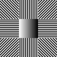
Refer to caption
(a) original
Refer to caption
(b) cartoon u1subscript𝑢1u_{1}
Refer to caption
(c) angle=0angle0\text{angle}=0, u2subscript𝑢2u_{2}
Refer to caption
(d) angle=π4angle𝜋4\text{angle}=\frac{\pi}{4}, u3subscript𝑢3u_{3}
Refer to caption
(e) angle=π2angle𝜋2\text{angle}=\frac{\pi}{2}, u4subscript𝑢4u_{4}
Refer to caption
(f) angle=3π4angle3𝜋4\text{angle}=\frac{3\pi}{4}, u5subscript𝑢5u_{5}
Refer to caption
(g) noisy image
Refer to caption
(h) restored image
Figure 3: Decomposition/denoising of a synthetic image. (a) Original image of dimensions 192×192192192192\times 192; (b) Cartoon component of the image; (c)–(f) The four directional texture components. Parameter choice: α1=0.06,β1=2α1,γ1=0,αi=0.5α1,βi=2αi,γi=0,i=2,,5formulae-sequencesubscript𝛼10.06formulae-sequencesubscript𝛽12subscript𝛼1formulae-sequencesubscript𝛾10formulae-sequencesubscript𝛼𝑖0.5subscript𝛼1formulae-sequencesubscript𝛽𝑖2subscript𝛼𝑖formulae-sequencesubscript𝛾𝑖0𝑖25\alpha_{1}=0.06,\beta_{1}=2\alpha_{1},\gamma_{1}=0,\alpha_{i}=0.5\alpha_{1},\beta_{i}=2\alpha_{i},\gamma_{i}=0,i=2,\ldots,5. (g) Noisy image corrupted by Gaussian noise with zero mean and standard deviation σ=0.1𝜎0.1\sigma=0.1; (h) Image restored by model (44). Parameter choice: α1=0.12,β1=2α1,γ1=0,αi=0.5α1,βi=2αi,γi=0.4αi,i=2,,5formulae-sequencesubscript𝛼10.12formulae-sequencesubscript𝛽12subscript𝛼1formulae-sequencesubscript𝛾10formulae-sequencesubscript𝛼𝑖0.5subscript𝛼1formulae-sequencesubscript𝛽𝑖2subscript𝛼𝑖formulae-sequencesubscript𝛾𝑖0.4subscript𝛼𝑖𝑖25\alpha_{1}=0.12,\beta_{1}=2\alpha_{1},\gamma_{1}=0,\alpha_{i}=0.5\alpha_{1},\beta_{i}=2\alpha_{i},\gamma_{i}=0.4\alpha_{i},i=2,\ldots,5.
Refer to caption
(a) noise-free test image
Refer to caption
(b) noisy test image (σ=0.05𝜎0.05\sigma=0.05)
Refer to captionRefer to caption
(c) TV-G𝐺G-norm
Refer to captionRefer to caption
(d) TV-H1superscript𝐻1H^{-1}
Refer to captionRefer to caption
(e) Fra+LDCT
Refer to captionRefer to caption
(f) proposed
Refer to captionRefer to caption
(g) TV-G𝐺G-norm
Refer to captionRefer to caption
(h) TV-H1superscript𝐻1H^{-1}
Refer to captionRefer to caption
(i) Fra+LDCT
Refer to captionRefer to caption
(j) proposed
Figure 4: Comparison of cartoon/texture decomposition methods for a synthetic image. (a) A noise-free test image consisting of a cartoon part and textured regions (352×352352352352\times 352 pixels); (b) A noisy version of (a) with Gaussian noise of zero mean and variance σ=0.05𝜎0.05\sigma=0.05; (c)–(f) Decomposition results for the noise-free image (top: cartoon part, bottom: texture part); (g)–(j) Decomposition results for the noisy image. Parameter choice for the proposed model: α1=0.07,β1=2α1,γ1=0,αi=0.9α1,βi=αi,γi=0.1αi,i=2,,17formulae-sequencesubscript𝛼10.07formulae-sequencesubscript𝛽12subscript𝛼1formulae-sequencesubscript𝛾10formulae-sequencesubscript𝛼𝑖0.9subscript𝛼1formulae-sequencesubscript𝛽𝑖subscript𝛼𝑖formulae-sequencesubscript𝛾𝑖0.1subscript𝛼𝑖𝑖217\alpha_{1}=0.07,\beta_{1}=2\alpha_{1},\gamma_{1}=0,\alpha_{i}=0.9\alpha_{1},\beta_{i}=\alpha_{i},\gamma_{i}=0.1\alpha_{i},i=2,\ldots,17.

In Figure 4 we show the decomposition/denoising performance for a synthetic image with cartoon part and some textured regions in comparison to the TVTV\operatorname{TV}-G𝐺G-norm model [4], TVTV\operatorname{TV}-H1superscript𝐻1H^{-1} model [43] and the framelet/local discrete cosine transform (Fra+LDCT) model [21]. We performed experiments both for a noise-free and noisy image (with Gaussian noise of variance σ=0.05𝜎0.05\sigma=0.05). In the results, one can see that some cartoon components (such as edges) and undesired information (such as noise), appear in the texture parts of the TVTV\operatorname{TV}-G𝐺G-norm and TVTV\operatorname{TV}-H1superscript𝐻1H^{-1} model which do not appear in the Fra+LDCT and the proposed model. Comparing the cartoon components of all models, one can observe staircasing effects in the TVTV\operatorname{TV}-G𝐺G-norm, TVTV\operatorname{TV}-H1superscript𝐻1H^{-1} and Fra+LDCT model as well as some texture artifacts in the TVTV\operatorname{TV}-H1superscript𝐻1H^{-1} model. Due to the utilization of TGVTGV\operatorname{TGV} for the cartoon component, these artifacts do not appear in the ICTGVoscisuperscriptICTGVosci\operatorname{ICTGV}^{\operatorname{osci}} model. Focusing on the texture component, both Fra+LDCT and the proposed model yield high-quality results. In the Fra+LDCT results, however, one can, for instance, see some low-frequency components in the trousers that are attributable to a shading and hence, should belong to the cartoon part. In contrast, the proposed ICTGVoscisuperscriptICTGVosci\operatorname{ICTGV}^{\operatorname{osci}} model does correctly assign these shadings to the cartoon part. Moreover, the boundaries of the texture seem to be better delineated in the proposed model compared to Fra+LDCT decomposition which shows some spill-over effects in the texture part. In summary, one can observe that the ICTGVoscisuperscriptICTGVosci\operatorname{ICTGV}^{\operatorname{osci}} decomposition/denoising model is effective in separating cartoon, texture and noise.

We also performed numerical experiments for the denoising of three natural images (“barbara”, “zebra” and “parrots”) and two different noise levels (Gaussian noise with zero mean and standard deviation σ=0.05𝜎0.05\sigma=0.05 and 0.10.10.1, respectively). The “barbara” and “zebra” test images have plentiful textures, some of which are large scale and some are small. They can be interpreted as different frequency components, so we used the ICTGVoscisuperscriptICTGVosci\operatorname{ICTGV}^{\operatorname{osci}}-model with sixteen texture components according to Remark 4, i.e., m=17𝑚17m=17 for these images. For the “parrots” image, we performed the experiments with eight texture components, i.e., m=9𝑚9m=9.

The results were compared to a selection of popular and state-of-the-art variational image models: TGVTGV\operatorname{TGV} of second order, non-local TVTV\operatorname{TV} (NLTV) [30, 53], ICTGV [33] as well as framelet/local DCT (Fra+LDCT) [21]. Additionally, we compared to BM3D [25] which is a dedicated denoising method. For all models, we manually tuned the parameters to give the best peak signal-to-noise ratio (PSNR). However, as some methods tend to produce ghost artifacts for PSNR-optimal parameters, we also tuned parameters in order to yield visually pleasing results; at least from the subjective viewpoint of the authors (namely, the NLTV, ICTGV, Fra+LDCT and the proposed model). The PSNR and SSIM values of these experiments are reported in Tables 1 and 2, respectively.

noise level image TGV NLTV ICTGV Fra+LDCT BM3D proposed model
σ=0.05𝜎0.05\sigma=0.05 barbara 27.41 32.05 (31.28) 31.15 (30.33) 31.70 (31.19) 34.43 32.21 (31.44)
zebra 28.74 31.16 (30.07) 31.08 (30.43) 30.81 (30.06) 32.25 31.33 (30.46)
parrots 34.77 35.10 (34.08) 36.49 (35.63) 36.10 (35.49) 37.40 36.61 (36.01)
σ=0.1𝜎0.1\sigma=0.1 barbara 25.34 27.58 (27.15) 27.35 (26.71) 28.05 (27.66) 31.06 28.45 (27.89)
zebra 25.24 27.35 (26.93) 27.35 (26.83) 27.06 (26.44) 28.80 27.65 (27.00)
parrots 32.51 31.39 (30.13) 33.28 (32.35) 32.91 (32.65) 34.08 33.32 (32.70)
Table 1: Comparison of denoising performance for noise levels σ=0.05𝜎0.05\sigma=0.05 and σ=0.1𝜎0.1\sigma=0.1 in terms of PSNR. (The values in parentheses correspond to the visually-optimized results.)
noise level image TGV NLTV ICTGV Fra+LDCT BM3D proposed model
σ=0.05𝜎0.05\sigma=0.05 barbara 0.8043 0.9005 (0.8917) 0.8859 (0.8833) 0.8857 (0.8988) 0.9365 0.9004 (0.8988)
zebra 0.8386 0.8647 (0.8419) 0.8761 (0.8735) 0.8653 (0.8671) 0.8998 0.8859 (0.8777)
parrots 0.9157 0.8956 (0.9062) 0.9324 (0.9272) 0.9259 (0.9257) 0.9416 0.9358 (0.9303)
σ=0.1𝜎0.1\sigma=0.1 barbara 0.7297 0.7553 (0.7814) 0.7835 (0.7840) 0.8214 (0.8201) 0.8920 0.8235 (0.8120)
zebra 0.7472 0.7271 (0.7540) 0.7796 (0.7897) 0.7868 (0.7795) 0.8237 0.7965 (0.7948)
parrots 0.8887 0.8312 (0.8530) 0.8975 (0.8889) 0.8903 (0.8928) 0.9025 0.8979 (0.8936)
Table 2: Comparison of denoising performance for noise levels σ=0.05𝜎0.05\sigma=0.05 and σ=0.1𝜎0.1\sigma=0.1 in terms of SSIM. (The values in parentheses correspond to the visually-optimized results.)
Refer to captionRefer to caption
(a) ground truth
Refer to captionRefer to caption
(b) noisy image (σ=0.05𝜎0.05\sigma=0.05)
Refer to captionRefer to caption
(c) TGV
Refer to captionRefer to caption
(d) NLTV
Refer to captionRefer to caption
(e) ICTGVICTGV\operatorname{ICTGV}
Refer to captionRefer to caption
(f) Fra+LDCT
Refer to captionRefer to caption
(g) BM3D
Refer to captionRefer to caption
(h) proposed model
Figure 5: Denoising results for barbara image with noise level σ=0.05𝜎0.05\sigma=0.05. All parameters are tuned for visually-optimal results. Parameter choice for the proposed model: α1=0.05,β1=α1,γ1=0,αi=0.9α1,βi=αi,γi=0.1αi,i=2,,17formulae-sequencesubscript𝛼10.05formulae-sequencesubscript𝛽1subscript𝛼1formulae-sequencesubscript𝛾10formulae-sequencesubscript𝛼𝑖0.9subscript𝛼1formulae-sequencesubscript𝛽𝑖subscript𝛼𝑖formulae-sequencesubscript𝛾𝑖0.1subscript𝛼𝑖𝑖217\alpha_{1}=0.05,\beta_{1}=\alpha_{1},\gamma_{1}=0,\alpha_{i}=0.9\alpha_{1},\beta_{i}=\alpha_{i},\gamma_{i}=0.1\alpha_{i},i=2,\ldots,17.

Figure 12 shows an example of the denoising performance of the methods on the “barbara” test image with noise level σ=0.05𝜎0.05\sigma=0.05 in detail. Additionally, the outcome of the ICTGVoscisuperscriptICTGVosci\operatorname{ICTGV}^{\operatorname{osci}}-denoising for all tests is presented in Figure 6. For the remaining results, we refer to the supplementary material (Section A).

Refer to captionRefer to caption
(a) barbara (σ=0.05𝜎0.05\sigma=0.05)
Refer to captionRefer to caption
(b) zebra (σ=0.05𝜎0.05\sigma=0.05)
Refer to captionRefer to caption
(c) parrots (σ=0.05𝜎0.05\sigma=0.05)
Refer to captionRefer to caption
(d) barbara (σ=0.1𝜎0.1\sigma=0.1)
Refer to captionRefer to caption
(e) zebra (σ=0.1𝜎0.1\sigma=0.1)
Refer to captionRefer to caption
(f) parrots (σ=0.1𝜎0.1\sigma=0.1)
Figure 6: Results of ICTGVoscisuperscriptICTGVosci\operatorname{ICTGV}^{\operatorname{osci}}-denoising for natural images at different noise levels. For more details and comparisons, see the supplemental material.

One can see in Figure 12 that the proposed model is able to preserve more textures than the TGV model alone which is designed for piecewise smooth functions but does not specifically take textures into account. In contrast, NLTV is, due to its non-local nature, able to reconstruct parts of the texture. It suffers, however, from the staircasing behaviour that is typical for TV-like approaches. The Fra+LDCT and BM3D method yield smoother reconstructions in pure cartoon regions while also capturing the texture very well. They suffer, however, from ghosting artifacts in the smooth regions which leads, for instance, to a unnatural appearance of the face in the “barbara” image. The ICTGV model does not show these artifacts, but the texture denoising is not very well, see the trousers of the “barbara” image, where the line-like textures still look irregular. In comparison, the proposed ICTGVoscisuperscriptICTGVosci\operatorname{ICTGV}^{\operatorname{osci}} model is able to capture both the texture and the smooth regions without producing ghosting artifacts. Nevertheless, for very fine textures, such as on the left trouser of the “barbara” image, the Fra+LDCT and BM3D approaches still reconstruct more of the details. This might be the reason for BM3D slightly outperforming the proposed methods in terms of quantitative measures (see Tables 1 and 2). The BM3D method is, however, specifically optimized for denoising and not variational, such that a generalization to inverse problems is not immediate. Among the variational approaches, the ICTGVoscisuperscriptICTGVosci\operatorname{ICTGV}^{\operatorname{osci}} model performs best in terms of quantitative measures.

Convergence graphs that show the evolution of the root mean square error (RMSE) for TGV, ICTGV and ICTGVoscisuperscriptICTGVosci\operatorname{ICTGV}^{\operatorname{osci}} (m=9,17𝑚917m=9,17) in terms of iteration number and computation time (with respect to GPU-supported MATLAB implementations) can be found in Figure 7. The experiments were performed for denoising the “barbara” image (dimensions 720×576720576720\times 576) and with primal-dual methods for TGV and ICTGV that are similar to Algorithm 1. One can see that the essential improvement of the RMSE is achieved, for all methods, in a few hundreds of iterations and within 30 seconds, respectively. From a practical point of view this means that the proposed model and algorithm quickly improves image quality. However, these results stem from an interplay between model and algorithm, and there might be more efficient algorithms for the same model for which the behaviour is different in terms of RMSE improvement. Finally, to give an overview of the computational complexity, we also ran each algorithm with 2000 iterations for three times and took the average of the computation time, see, again Figure 7.
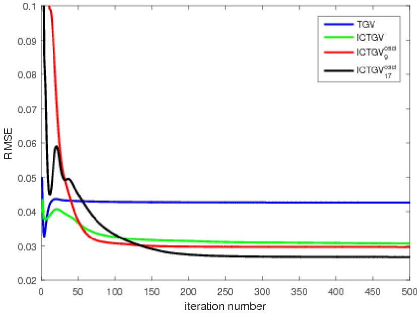
Refer to caption

(a)

Refer to caption

(b)

method time TGV 114.83s ICTGV 104.46s ICTGVoscisuperscriptICTGVosci\operatorname{ICTGV}^{\operatorname{osci}} (m=9𝑚9m=9) 187.89s ICTGVoscisuperscriptICTGVosci\operatorname{ICTGV}^{\operatorname{osci}} (m=17𝑚17m=17) 164.97s

(c)

Figure 7: Convergence graph and computational complexity of TGV, ICTGV and ICTGVoscisuperscriptICTGVosci\operatorname{ICTGV}^{\operatorname{osci}} for “barbara” image with noise level σ=0.05𝜎0.05\sigma=0.05. (a) the RMSE values versus iterations; (b) the RMSE values versus GPU time; (c) the computation time (GPU) with 2000 iterations.

Finally, the supplementary material also contains a comparison for the “barbara” image with a varying number of oscillation directions in the extended model, i.e., 4, 6, 8, 10 and 12 directions (Section A.3). There, one can see that the restored images with 4 and 6 directions lose some textures, whereas the majority of textures is recovered using 8, 10 and 12 directions. Hence, the choice of 8 directions in (38) indeed offers a good balance between performance and complexity of the model.

5.2 Image inpainting

Inpainting, i.e., the restoration of missing regions of an image, is a well-studied standard image processing problem. It can, for example, be used to repair corruptions in digital photos or in ancient drawings, and to fill in the missing pixels of images transmitted through a noisy channel. In this subsection, we will apply the new regularizer to a restoration problem where pixels are missing randomly with a certain rate. We model this situation as follows. For ΩΩ\Omega the image domain, let ΩΩsuperscriptΩΩ\Omega^{\prime}\subset\Omega the non-empty subdomain on which data is not missing. Given fL2(Ω)𝑓superscript𝐿2superscriptΩf\in L^{2}(\Omega^{\prime}), we are seeking a uL2(Ω)superscript𝑢superscript𝐿2Ωu^{*}\in L^{2}(\Omega) that minimizes ICTGVoscisuperscriptICTGVosci\operatorname{ICTGV}^{\operatorname{osci}} in the variant that promotes sparse textures. In terms of the operator K:L2(Ω)L2(Ω):𝐾superscript𝐿2Ωsuperscript𝐿2superscriptΩK:L^{2}(\Omega)\to L^{2}(\Omega^{\prime}), Ku=u|Ω𝐾𝑢evaluated-at𝑢superscriptΩKu=u|_{\Omega^{\prime}} projecting u𝑢u to the non-corrupted region, this corresponds to solving

minuL2(Ω)ICTGVα,β,𝐜,γosci(u)subject toKu=f.subscript𝑢superscript𝐿2ΩsubscriptsuperscriptICTGVosci𝛼𝛽𝐜𝛾𝑢subject to𝐾𝑢𝑓\min_{u\in L^{2}(\Omega)}\ \operatorname{ICTGV}^{\operatorname{osci}}_{\vec{\alpha},\vec{\beta},\vec{\mathbf{c}},\vec{\gamma}}(u)\quad\text{subject to}\quad Ku=f. (45)

Proposition 6 applied to F={f}𝐹subscript𝑓F=\mathcal{I}_{\{f\}} and Φ=ICTGVα,β,𝐜,γosciΦsubscriptsuperscriptICTGVosci𝛼𝛽𝐜𝛾\Phi=\operatorname{ICTGV}^{\operatorname{osci}}_{\vec{\alpha},\vec{\beta},\vec{\mathbf{c}},\vec{\gamma}} yields existence in this situation. In order to solve (45), one can use a slightly modified version of Algorithm 1: Note that the only difference between the discrete version of this model and the version (40) is the fidelity term, where the term Ki=1muif,λλ22𝐾superscriptsubscript𝑖1𝑚subscript𝑢𝑖𝑓𝜆superscriptnorm𝜆22\langle K\sum\limits_{i=1}\limits^{m}u_{i}-f,\lambda\rangle-\frac{\|\lambda\|^{2}}{2} is replaced by Ki=1muif,λ𝐾superscriptsubscript𝑖1𝑚subscript𝑢𝑖𝑓𝜆\langle K\sum\limits_{i=1}\limits^{m}u_{i}-f,\lambda\rangle. Thus, λ𝜆\lambda in Algorithm 1 is updated according to
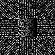
λn+1=λn+σ(Ki=1mu¯inf).superscript𝜆𝑛1superscript𝜆𝑛𝜎𝐾superscriptsubscript𝑖1𝑚superscriptsubscript¯𝑢𝑖𝑛𝑓\lambda^{n+1}=\lambda^{n}+\sigma\Bigl{(}K\sum\limits_{i=1}\limits^{m}\bar{u}_{i}^{n}-f\Bigr{)}.
Refer to caption
(a) 60%percent6060\% missing
Refer to caption
(b) 75%percent7575\% missing
Refer to caption
(c) 90%percent9090\% missing
Refer to caption
(d) inpainted image
Refer to caption
(e) inpainted image
Refer to caption
(f) inpainted image
Figure 8: Inpainting results for a synthetic image (192×192192192192\times 192 pixels). (a)–(c) Corrupted image with 60%percent6060\%, 75%percent7575\% and 90%percent9090\% pixels missing, respectively; (d)–(f) Images inpainted by model (45). Parameter choice: α1=0.04,β1=α1,γ1=0,αi=α1,βi=0.5αi,γi=0.02αi,i=2,,5formulae-sequencesubscript𝛼10.04formulae-sequencesubscript𝛽1subscript𝛼1formulae-sequencesubscript𝛾10formulae-sequencesubscript𝛼𝑖subscript𝛼1formulae-sequencesubscript𝛽𝑖0.5subscript𝛼𝑖formulae-sequencesubscript𝛾𝑖0.02subscript𝛼𝑖𝑖25\alpha_{1}=0.04,\beta_{1}=\alpha_{1},\gamma_{1}=0,\alpha_{i}=\alpha_{1},\beta_{i}=0.5\alpha_{i},\gamma_{i}=0.02\alpha_{i},i=2,\ldots,5.

We performed numerical experiments using the inpainting model (45) and the described modification of Algorithm 1. Our first experiment aimed at recovering the synthetic image already utilized in the decomposition/denoising experiments, see Figure 3. In this experiment, 60%, 75% and 90% of the pixels were randomly removed from the image and inpainted by ICTGVoscisuperscriptICTGVosci\operatorname{ICTGV}^{\operatorname{osci}}-minimization. The results are shown in Figure 8. There, one can see that the recovery from 60% and 75% of the missing pixels is almost perfect; whereas for 90% of missing pixels, the texture is also perfectly recovered while the boundaries of the regions deviate from the ground truth. The latter may be explained by the fact that in this situation, not enough data is available to unambiguously reconstruct the boundaries. In contrast, there is still enough information to determine the respective parameters of the affine and oscillatory parts. Overall, the experiment shows that ICTGVoscisuperscriptICTGVosci\operatorname{ICTGV}^{\operatorname{osci}}-regularization is able to effectively reconstruct oscillatory texture in inpainting problems.

Further, experiments with natural images (“barbara”, “zebra” and “fish”) were carried out. For these images, we also performed a comparison to TGV of second order and the framelet/local DCT model. Figure 27 shows a comparison of the inpainting performances for selected examples; we refer to the supplementary material Section B for more detailed results. Again, for the “barbara” and “zebra” image, sixteen texture components were used, i.e., m=17𝑚17m=17, and for the “fish” image, experiments were performed with eight texture directions, i.e., m=9𝑚9m=9. One can clearly see in Figure 27 that our proposed model is able to restore the corrupted images in high quality with the majority of the textures being recovered, such as, for instance, the table cloth and the scarf in the “barbara” image as well as the stripes on the bodies of the zebra and the fish. The same holds for the Fra+LDCT-based model while the TGV-model does not recover well the texture and leaves many unconnected “speckles”. The latter is typical for derivative- and measure-based models and does also apply, e.g., to TVTV\operatorname{TV}-inpainting. Furthermore, Tables 12 and 4 show the PSNR and SSIM values of the three models at different rates of missing pixels. As we see, the proposed model performs better than other two models by these two evaluation standards. However, despite the favorable quantitative comparison to Fra+LDCT model, the proposed model has only limited ability of recovering textures of very high frequency. Looking at the left trouser in the “barbara” image near the arm, there are some textures that are not inpainted correctly. In contrast, in the result of Fra+LDCT-model, this region is recovered well.
Refer to captionRefer to caption
(a) 50%percent5050\% missing
Refer to captionRefer to caption
(b) TGV
Refer to captionRefer to caption
(c) Fra+LDCT
Refer to captionRefer to caption
(d) proposed model
Refer to captionRefer to caption
(e) 50%percent5050\% missing
Refer to captionRefer to caption
(f) TGV
Refer to captionRefer to caption
(g) Fra+LDCT
Refer to captionRefer to caption
(h) proposed model
Refer to captionRefer to caption
(i) 50%percent5050\% missing
Refer to captionRefer to caption
(j) TGV
Refer to captionRefer to caption
(k) Fra+LDCT
Refer to captionRefer to caption
(l) proposed model
Figure 9: Inpainting results for “barbara”, “zebra” and “fish” image. (a)–(d), (e)–(h), (i)–(l): Reconstruction from 50% missing pixels for proposed and reference methods for the respective test images. For more details and results, see the supplementary material.
image TGV Fra+LDCT proposed model
50%percent5050\% 60%percent6060\% 70%percent7070\% 50%percent5050\% 60%percent6060\% 70%percent7070\% 50%percent5050\% 60%percent6060\% 70%percent7070\%
barbara 27.49 26.26 25.09 32.75 30.76 28.53 34.03 31.86 29.49
zebra 26.00 24.23 22.65 28.50 26.67 25.08 30.09 28.11 26.42
fish 22.70 20.81 19.01 24.54 23.01 21.22 25.10 23.50 21.54
Table 3: Comparison of inpainting performance for different rates of missing pixels in terms of PSNR.
image TGV Fra+LDCT proposed model
50%percent5050\% 60%percent6060\% 70%percent7070\% 50%percent5050\% 60%percent6060\% 70%percent7070\% 50%percent5050\% 60%percent6060\% 70%percent7070\%
barbara 0.8942 0.8562 0.8081 0.9549 0.9320 0.8953 0.9591 0.9390 0.9078
zebra 0.9016 0.8597 0.8051 0.9213 0.8863 0.8438 0.9463 0.9194 0.8839
fish 0.8676 0.8059 0.7255 0.8923 0.8462 0.7902 0.9059 0.8596 0.7977
Table 4: Comparison of inpainting performance for different rates of missing pixels in terms of SSIM.

5.3 Undersampled magnetic resonance imaging

Since compressed sensing techniques have been shown to be effective for image reconstruction in magnetic resonance imaging (MRI) with undersampling [40, 41], i.e., where much less data is available than usually required, variational methods were becoming increasingly popular for undersampling MRI [35, 6, 36] in particular and medical image processing in general. As MRI samples data in the Fourier domain, it is particularly well-suited for these methods. In this subsection, we discuss ICTGVoscisuperscriptICTGVosci\operatorname{ICTGV}^{\operatorname{osci}}-regularization for recovering an image given incomplete Fourier data. We model the situation as follows. Let Ω2Ωsuperscript2\Omega\subset\mathbb{R}^{2} be a bounded image domain and (Ω,μ)superscriptΩ𝜇(\Omega^{\prime},\mu) a finite Borel measure space on a bounded Ω2superscriptΩsuperscript2\Omega^{\prime}\subset\mathbb{R}^{2}, where ΩsuperscriptΩ\Omega^{\prime} represents the set of measured Fourier data. The restriction of the Fourier transform 𝒫𝒫\mathcal{PF} then maps L2(Ω)L2(Ω,μ)superscript𝐿2Ωsuperscript𝐿2superscriptΩ𝜇L^{2}(\Omega)\to L^{2}(\Omega^{\prime},\mu) since both ΩΩ\Omega and ΩsuperscriptΩ\Omega^{\prime} are bounded and the Fourier transform \mathcal{F} on the whole space maps L1(2)superscript𝐿1superscript2L^{1}(\mathbb{R}^{2}) functions to continuous functions on 2superscript2\mathbb{R}^{2}. Given fL2(Ω,μ)𝑓superscript𝐿2superscriptΩ𝜇f\in L^{2}(\Omega^{\prime},\mu), the undersampled MRI reconstruction corresponds to solving Ku=f𝐾𝑢𝑓Ku=f for K=𝒫𝐾𝒫K=\mathcal{PF}, such that the ICTGVoscisuperscriptICTGVosci\operatorname{ICTGV}^{\operatorname{osci}}-regularized solution (in its sparse-texture variant) reads as

minuL2(Ω)12Ω|Kuf|2dμ+ICTGVα,β,𝐜,γosci(u).subscript𝑢superscript𝐿2Ω12subscriptsuperscriptΩsuperscript𝐾𝑢𝑓2differential-d𝜇subscriptsuperscriptICTGVosci𝛼𝛽𝐜𝛾𝑢\min_{u\in L^{2}(\Omega)}\ \frac{1}{2}\int_{\Omega^{\prime}}|{Ku-f}|^{2}\,\mathrm{d}{\mu}+\operatorname{ICTGV}^{\operatorname{osci}}_{\vec{\alpha},\vec{\beta},\vec{\mathbf{c}},\vec{\gamma}}(u). (46)

Clearly, the problem (46) admits a solution, see Theorem 2. In applications, the Borel measure space (Ω,μ)superscriptΩ𝜇(\Omega^{\prime},\mu) could, for instance, be Ω2superscriptΩsuperscript2\Omega^{\prime}\subset\mathbb{R}^{2} a bounded domain and μ=2𝜇superscript2\mu=\mathcal{L}^{2} the Lebesgue measure, ΩsuperscriptΩ\Omega^{\prime} a finite collection of line segments and μ=1Ω𝜇superscript1superscriptΩ\mu=\mathcal{H}^{1}\llcorner\Omega^{\prime} the one-dimensional Hausdorff measure restricted to ΩsuperscriptΩ\Omega^{\prime} (which models so-called radial sampling in case of radially centered line segments), or ΩsuperscriptΩ\Omega^{\prime} is a finite collection of points and μ=0Ω𝜇superscript0superscriptΩ\mu=\mathcal{H}^{0}\llcorner\Omega^{\prime} a collection of delta-measures (modelling compressed-sensing-inspired sampling).

For the discretization, we chose \mathcal{F} to represent the discrete Fourier transform on the discrete grid ΩΩ\Omega which is usually realized by a fast algorithm (FFT). Further, the discrete domain ΩsuperscriptΩ\Omega^{\prime} is chosen as ΩΩsuperscriptΩΩ\Omega^{\prime}\subset\Omega and 𝒫𝒫\mathcal{P} is the projection operator which restricts Fourier coefficients to ΩsuperscriptΩ\Omega^{\prime}. In total, K=𝒫𝐾𝒫K=\mathcal{PF} as in the continuous setting and Algorithm 1 can be used to compute a solution.

We performed numerical experiments for undersampled MRI with radial sampling patterns associated with a varying number of sampling lines; see Figure 10 for the illustration of a selection mask with 70 equispaced radial sampling lines which corresponds to a sampling rate of approximately 14.74%percent14.7414.74\% for an image of 512×512512512512\times 512 pixels.

Refer to caption
Figure 10: Example of a sampling pattern associated with radial sampling (70 equispaced radial lines, image resolution: 512×512512512512\times 512 pixels).

The experimental results for MR image reconstruction are shown in comparison to TGV-Shearlet MRI reconstruction in [32] which is based on simultaneous TGV and shearlet-transform-based regularization.

sampling lines 40 50 60 70 80 90 100
TGV-shearlet foot 30.81 32.59 33.75 34.99 36.51 37.34 38.59
knee 28.01 28.77 29.59 30.10 30.84 31.50 32.07
brain 34.05 35.71 37.18 38.44 39.66 40.51 41.43
proposed model foot 29.76 32.41 33.89 35.27 37.07 38.25 39.66
knee 28.40 29.16 29.98 30.56 31.23 31.82 32.36
brain 34.64 36.97 38.99 40.33 41.65 42.71 43.67
Table 5: Comparison of MRI reconstruction performance for different sampling rates in terms of PSNR.
sampling lines 40 50 60 70 80 90 100
TGV-shearlet foot 0.8451 0.8669 0.8823 0.8956 0.9098 0.9175 0.9262
knee 0.7356 0.7656 0.7950 0.8133 0.8348 0.8508 0.8661
brain 0.8867 0.9059 0.9209 0.9318 0.9408 0.9466 0.9523
proposed model foot 0.8653 0.9280 0.9465 0.9567 0.9702 0.9774 0.9822
knee 0.7581 0.7861 0.8148 0.8344 0.8570 0.8720 0.8878
brain 0.9055 0.9421 0.9600 0.9681 0.9743 0.9784 0.9818
Table 6: Comparison of MRI reconstruction performance for different sampling rates in terms of SSIM.

For the MRI reconstruction experiment, we chose some fully sampled MR test images from an online database (http://www.mr-tip.com/): a T1subscript𝑇1T_{1}-weighted foot image (512×512512512512\times 512 pixels) and a T1subscript𝑇1T_{1}-weighted knee image (350×350350350350\times 350 pixels); and a T2subscript𝑇2T_{2}-weighted brain image (490×490490490490\times 490 pixels) (image courtesy of A. Farrall, University of Edinburgh). Undersampled measurements were then synthetically created by restricting the Fourier coefficients to radial sampling lines where the number of lines covers the range 40,50,,100405010040,50,\ldots,100. Reconstructions were obtained from these measurements using the TGV+Shearlet model and by minimizing (46) where for both methods, parameters were tuned to yield optimal PSNR. Figure 28 shows exemplary results; see the supplementary material (Section C) for more detailed results. One can see in these results that both the TGV+Shearlet and the proposed model are able to preserve the textures well. Further, one can observe that the proposed model yields more naturally appearing bones and junctions that are also closer to the ground truth. The muscular tissues in the foot and knee image as well as the brain tissue are also reconstructed well. For the latter, the ICTGVoscisuperscriptICTGVosci\operatorname{ICTGV}^{\operatorname{osci}}-model also has a desired smoothing effect that reduces the ringing artifacts originating from the MR measurements. Furthermore, note that there are some ghost stripes in the results of TGV+Shearlet model which do not appear in the ICTGVoscisuperscriptICTGVosci\operatorname{ICTGV}^{\operatorname{osci}} approach. The quantitative comparison in terms of PSNR and SSIM, see Tables 13 and 14, support these findings. Except for the PSNR for the foot image at low sampling rates, the proposed method consistently outperforms the TGV+Shearlet approach with respect to these quantitative measures. The only weakness one might observe in both models may the found in the foot image: There, the ground truth admits several fine directional structures in the bone (see the closeup) for which the reconstructions do not correctly recover the orientations and artificially introduce vertical structures. This effect can, however, be mitigated by switching to the extended model (m=17𝑚17m=17) that also includes oscillations of higher frequencies, see the supplementary material.

Refer to captionRefer to caption
(a) ground truth
Refer to captionRefer to caption
(b) TGV+Shearlet
Refer to captionRefer to caption
(c) proposed model
Refer to captionRefer to caption
(d) ground truth
Refer to captionRefer to caption
(e) TGV+Shearlet
Refer to captionRefer to caption
(f) proposed model
Refer to captionRefer to caption
(g) ground truth
Refer to captionRefer to caption
(h) TGV+Shearlet
Refer to captionRefer to caption
(i) proposed model
Figure 11: Comparison of MRI reconstruction results. (a) Foot image; (b)–(c) Recovery from 14.74%percent14.7414.74\% radially sampled coefficients; (d) Knee image; (e)–(f) Recovery from 21.12%percent21.1221.12\% radially sampled coefficients; (g) Brain image; (h)–(i) Recovery from 13.47%percent13.4713.47\% radially sampled coefficients. See the supplementary material for more detailed results.

6 Summary and conclusions

In this paper, we proposed the oscillation TGV regularizer which arises from modifying the second-order TGV functional such that structured oscillatory functions are in its kernel. The infimal convolution of these novel regularization functionals can be used to represent structured texture consisting of oscillations of different directions and frequencies. We have shown that the natural space for oscillation TGV is the space of functions of bounded variation in the sense that norm equivalence, lower semi-continuity and coercivity can be established in that space. Furthermore, we considered the m𝑚m-fold infimal convolution of oscillation TGV which can be utilized for solving many variational image processing problems; in particular those for which TVTV\operatorname{TV}-regularization is applicable. The analysis of the infimal-convolution model based on general properties of infimal convolution of lower semi-continuous semi-norms. For such functionals, we obtained general criteria for exactness, lower semi-continuity and coercivity of the infimal convolution. This allowed us to obtain existence results for variational problems regularized with this type of functional. We discussed a possible discretization of the oscillation TGV functional. It turned out that one has to choose the 𝐜isubscript𝐜𝑖\mathbf{c}_{i} specifically in order to preserve the kernel in the discretized version. Numerical experiments for denoising, inpainting and MRI reconstruction show the major properties of the proposed model in terms of texture preservation and reconstruction. The general framework obtained in this article allows in particular the extension to other imaging problems. A possible line of future research may focus on reducing the complexity of the proposed model by studying variants of oscillation TGV that allow for reconstruction of oscillatory textures for multiple directions and frequencies with a simple, differentiation-based functional.

Acknowledgments

The first author is supported by China Scholarship Council (CSC) Scholarship Program and National Natural Science Foundation of China (Nos. 11531005 and 91330101). The second author acknowledges support by the Austrian Science Fund (FWF): project number P-29192 “Regularization Graphs for Variational Imaging”.

References

  • [1] L. Ambrosio, A. Coscia and G. Maso, Fine properties of functions with bounded deformation, Arch. Ration. Mech. Anal., 139 (1997), 201–238.
  • [2] L. Ambrosio, N. Fusco and D. Pallara, Functions of bounded variation and free discontinuity problems, Oxford University Press, Oxford, 2000.
  • [3] H. Attouch and H. Brezis, Duality for the sum of convex functions in general Banach spaces, In Aspects of Mathematics and its Applications, 34 (1986), 125–133.
  • [4] J. F. Aujol, G. Aubert, L. Blanc-Féraud and A. Chambolle, Image decomposition into a bounded variation component and an oscillating component and an oscillating component, J. Math. Imaging Vis., 22 (2005), 71–88.
  • [5] H. H. Bauschke and P. L. Combettes. Convex analysis and monotone operator theory in Hilbert spaces, New York: Springer, 2011.
  • [6] K. T. Block, M. Uecker and J. Frahm, Undersampled radial MRI with multiple coils. Iterative image reconstruction using a total variation constraint, Magnetic resonance in medicine, 57(6) (2007), 1086–1098.
  • [7] K. Bredies, Recovering piecewise smooth multichannel images by minimization of convex functionals with total generalized variation penalty, Lecture Notes in Computer Science, 8293 (2014), 44–77.
  • [8] K. Bredies and M. Holler, Artifact-Free Variational MPEG Decompression, Lecture Notes in Computer Science, 9087 (2015), 216–228.
  • [9] K. Bredies and M. Holler, A TGV-based framework for variational image decompression, zooming and reconstruction. Part I: Analytics, SIAM J. Imag. Sci., 8(4) (2015), 2814–2850.
  • [10] K. Bredies and M. Holler, A TGV-based framework for variational image decompression, zooming and reconstruction. Part II: Numerics, SIAM J. Imag. Sci., 8(4) (2015), 2851–2886.
  • [11] K. Bredies and M. Holler, Regularization of linear inverse problems with total generalized variation, Journal of Inverse and Ill-posed Problems, 22(6) (2014), 871–913.
  • [12] K. Bredies, K. Kunisch and T. Pock, Total generalized variation, SIAM J. Imag. Sci., 3 (2010), 492–526.
  • [13] K. Bredies and H. P. Sun, Preconditioned Douglas-Rachford algorithms for TV and TGV regularized variational imaging problems, J. Math. Imaging Vis., 52(3) (2015), 317–344.
  • [14] K. Bredies and T. Valkonen, Inverse problems with second-order total generalized variation constraints, In 9th International Conference on Sampling Theory and Applications, Singapore, 2011.
  • [15] A. Buades, B. Coll, and J. M. Morel, A review of image denoising algorithms, with a new one, Multiscale Model. Simul., 4(2) (2005), 490–530.
  • [16] A. Buades, B. Coll, and J. M. Morel, Neighborhood filters and PDE’s, Numer. Math., 105(1) (2006), 1–34.
  • [17] A. Buades, T. Le, J. M. Morel and L. Vese, Fast cartoon+texture image filters, IEEE Trans. Image Process., 19(8) (2010), 1978–1986.
  • [18] A. Buades and J. L. Lisani, Directional filters for color cartoon+texture image and video decomposition, J. Math. Imaging Vis., 55 (2016), 125–135.
  • [19] M. Burger, G. Gilboa, M. Moeller, L. Eckardt and D. Cremers, Spectral decompositions using one-homogeneous functionals, SIAM J. Imag. Sci., 9(3) (2016), 1374–1408.
  • [20] J. F. Cai, R. H. Chan, and Z. W. Shen, A framelet-based image inpainting algorithm, Appl. Comput. Harmon. Anal., 24 (2008), 131–149.
  • [21] J. F. Cai, S. Osher, and Z. W. Shen, Split Bregman methods and frame based image restoration, Multiscale Model. Simul., 8(2) (2009), 337–369.
  • [22] E. J. Candès, X. Li, Y. Ma, and J. Wright, Robust principal component analysis?, Journal of the ACM, 58(3) (2011), 11.
  • [23] A. Chambolle, An algorithm for total variation minimization and applications, J. Math. Imaging Vis., 20 (2004), 89–97.
  • [24] A. Chambolle and T. Pock, A first-order primal-dual algorithm for convex problems with applications to imaging, J. Math. Imaging Vis., 40 (2011), 120–145.
  • [25] K. Dabov, A. Foi, V. Katkovnik, and K. Egiazarian, Image Denoising by Sparse 3D Transform-Domain Collaborative Filtering, IEEE Trans. Image Processing, 16(8) (2007), 2080–2095.
  • [26] I. Ekeland and R. Témam, Convex Analysis and Variational Problems, Classics Appl. Math. 28, SIAM, Philadelphia, 1999.
  • [27] M. Elad, J. L. Starck, P. Querre, and D. L. Donoho, Simultaneous cartoon and texture image inpainting using morphological component analysis (MCA), Appl. Comput. Harmon. Anal., 19 (2005), 340–358.
  • [28] G. Gilboa, A spectral approach to total variation, Scale Space and Variational Methods, SSVM 2013, LNCS 7893(2013), 36–47.
  • [29] G. Gilboa, A total variation spectral framework for scale and texture analysis, SIAM J. Imag. Sci., 7(4) (2014), 1937–1961.
  • [30] G. Gilboa and S. Osher, Nonlocal operators with applications to image processing, Multiscale Model. Simul., 7(3) (2008), 1005–1028.
  • [31] E. Giusti, Minimal surfaces and functions of bounded variation, Birkhäuser, Boston, 1984.
  • [32] W. H. Guo, J. Qin and W. T. Yin, A new detail-preserving regularization scheme, SIAM J. Imag. Sci., 7(2) (2014), 1309–1334.
  • [33] M. Holler and K. Kunisch, On infimal convolution of TV-type functionals and applications to video and image reconstruction, SIAM J. Imag. Sci., 7(4) (2014), 2258–2300.
  • [34] D. Horesh and G. Gilboa, Separation surfaces in the spectral TV domain for texture decomposition, IEEE Trans. Image Processing, 25(9) (2016), 4260–4270.
  • [35] F. Knoll, K. Bredies, T. Pock, and R. Stollberger, Second order total generalized variation (TGV) for MRI, Magnetic Resonance in Medicine, 65(2) (2011), 480–491.
  • [36] F. Knoll, C. Clason, K. Bredies, M. Uecker and R. Stollberger, Parallel Imaging with Nonlinear Reconstruction using Variational Penalties, Magnetic resonance in medicine, 67(1) (2012), 34–41.
  • [37] F. Knoll, M. Holler, T. Koesters, R. Otazo, K. Bredies and D. K. Sodickson, Joint MR-PET reconstruction using a multi-channel image regularizer, IEEE Transactions on Medical Imaging, 36(1) (2017), 1–16.
  • [38] R. D. Kongskov and Y. Q. Dong, Directional Total Generalized Variation Regularization for Impulse Noise Removal, Scale Space and Variational Methods, SSVM 2017, 221–231.
  • [39] C. Langkammer, K. Bredies and B. Poser et al., Fast quantitative susceptibility mapping using 3D EPI and total generalized variation, NeuroImage, 111 (2015), 622–630.
  • [40] M. Lustig, D. Donoho and J. M. Pauly, Sparse MRI: The application of compressed sensing for rapid MR imaging, Magnetic resonance in medicine, 58(6) (2007), 1182–1195.
  • [41] M. Lustig, D. Donoho, J. M. Santos and J. M. Pauly, Compressed sensing MRI, IEEE Signal Processing Magazine, 25(2) (2008), 72–82.
  • [42] Y. Meyer, Oscillating patterns in image processing and in some nonlinear evolution equations, The 15th Dean Jacquelines B. Lewis Memorial Lectures, 2001.
  • [43] S. Osher, A. Sole, and L.A. Vese, Image decomposition and restoration using total variation minimization and the H1superscript𝐻1H^{-1} norm, Multiscale Model. Simul., 1(2) (2003), 349–370.
  • [44] R. Ranftl, K. Bredies and T. Pock, Non-local total generalized variation for optical flow estimation, In: Computer Vision–ECCV 2014, Lecture Notes in Computer Science, 8689:439–454.
  • [45] R. T. Rockafellar, Convex analysis, Princeton Landmarks in Mathematics, Princeton University Press, Princeton, NJ, 1997. Reprint of the 1970 original, Princeton Paperbacks.
  • [46] L. Rudin, S. Osher and E. Fatemi, Nonlinear total variation based noise removal algorithms, Phys. D, 60 (1992), 61–79.
  • [47] H. Schaeffer and S. Osher, A low patch-rank interpretation of texture, SIAM J. Imag. Sci., 6(1) (2013), 226–262.
  • [48] M. Schloegl, M. Holler, A. Schwarzl, K. Bredies and R. Stollberger, Infimal Convolution of Total Generalized Variation Functionals for dynamic MRI, Magnetic Resonance in Medicine, 78(1) (2017), 142–155.
  • [49] J. L. Starck, M. Elad, and D. L. Donoho, Image decomposition via the combination of sparse representations and a variational approach, IEEE Trans. Image Process., 14 (2005), 1570–1582.
  • [50] R. Temam and G. Strang, Functions of bounded deformation, Arch. Ration. Mech. Anal., 75(1) (1980), 7–21.
  • [51] T. Valkonen, K. Bredies and F. Knoll, Total generalized variation in diffusion tensor imaging, SIAM J. Imag. Sci., 6 (2013), 487–525.
  • [52] L. Vese and S. Osher, Modeling textures with total variation minimization and oscillating patterns in image processing, J. Sci. Comput., 19 (2003), 553–577.
  • [53] X. Q. Zhang, M. Burger, X. Bresson and S. Osher, Bregmanized nonlocal regularization for deconvolution and sparse reconstruction, SIAM J. Imag. Sci., 3(3) (2010), 253–276.

Supplementary material

Appendix A Image denoising

A.1 Comparison of PSNR-optimal results

A.1.1 Noise level σ=0.05𝜎0.05\sigma=0.05

See Figures 1213 and 14, and Table 7.

image TGV NLTV ICTGV Fra+LDCT BM3D proposed model
PSNR barbara 27.41 32.05 31.15 31.70 34.43 32.21
zebra 28.74 31.16 31.08 30.81 32.25 31.33
parrots 34.77 35.10 36.49 36.10 37.40 36.61
SSIM barbara 0.8043 0.9005 0.8859 0.8857 0.9365 0.9004
zebra 0.8386 0.8647 0.8761 0.8653 0.8998 0.8859
parrots 0.9157 0.8956 0.9324 0.9259 0.9416 0.9358
Table 7: Comparison of denoising performance of PSNR-optimized results with noise level σ=0.05𝜎0.05\sigma=0.05 in terms of PSNR and SSIM.
Refer to captionRefer to caption
(a) ground truth
Refer to captionRefer to caption
(b) noisy image (σ=0.05𝜎0.05\sigma=0.05)
Refer to captionRefer to caption
(c) TGV
Refer to captionRefer to caption
(d) NLTV
Refer to captionRefer to caption
(e) ICTGVICTGV\operatorname{ICTGV}
Refer to captionRefer to caption
(f) Fra+LDCT
Refer to captionRefer to caption
(g) BM3D
Refer to captionRefer to caption
(h) proposed model
Figure 12: Denoising results for “barbara” image (720×576720576720\times 576 pixels) with noise level σ=0.05𝜎0.05\sigma=0.05. Parameter choice for ICTGVoscisuperscriptICTGVosci\operatorname{ICTGV}^{\operatorname{osci}}: α1=0.045,β1=0.7α1,γ1=0,αi=0.9α1,βi=0.6αi,γi=0.1αi,i=2,,17.formulae-sequencesubscript𝛼10.045formulae-sequencesubscript𝛽10.7subscript𝛼1formulae-sequencesubscript𝛾10formulae-sequencesubscript𝛼𝑖0.9subscript𝛼1formulae-sequencesubscript𝛽𝑖0.6subscript𝛼𝑖formulae-sequencesubscript𝛾𝑖0.1subscript𝛼𝑖𝑖217\alpha_{1}=0.045,\beta_{1}=0.7\alpha_{1},\gamma_{1}=0,\alpha_{i}=0.9\alpha_{1},\beta_{i}=0.6\alpha_{i},\gamma_{i}=0.1\alpha_{i},i=2,\ldots,17.
Refer to captionRefer to caption
(a) ground truth
Refer to captionRefer to caption
(b) noisy image (σ=0.05𝜎0.05\sigma=0.05)
Refer to captionRefer to caption
(c) TGV
Refer to captionRefer to caption
(d) NLTV
Refer to captionRefer to caption
(e) ICTGV
Refer to captionRefer to caption
(f) Fra+LDCT
Refer to captionRefer to caption
(g) BM3D
Refer to captionRefer to caption
(h) proposed model
Figure 13: Denoising results for “zebra” image (640×400640400640\times 400 pixels) with noise level σ=0.05𝜎0.05\sigma=0.05. Parameter choice for ICTGVoscisuperscriptICTGVosci\operatorname{ICTGV}^{\operatorname{osci}}: α1=0.045,β1=0.6α1,γ1=0,αi=α1,βi=0.5αi,γi=0.1αi,i=2,,17formulae-sequencesubscript𝛼10.045formulae-sequencesubscript𝛽10.6subscript𝛼1formulae-sequencesubscript𝛾10formulae-sequencesubscript𝛼𝑖subscript𝛼1formulae-sequencesubscript𝛽𝑖0.5subscript𝛼𝑖formulae-sequencesubscript𝛾𝑖0.1subscript𝛼𝑖𝑖217\alpha_{1}=0.045,\beta_{1}=0.6\alpha_{1},\gamma_{1}=0,\alpha_{i}=\alpha_{1},\beta_{i}=0.5\alpha_{i},\gamma_{i}=0.1\alpha_{i},i=2,\ldots,17.
Refer to captionRefer to caption
(a) ground truth
Refer to captionRefer to caption
(b) noisy image (σ=0.05𝜎0.05\sigma=0.05)
Refer to captionRefer to caption
(c) TGV
Refer to captionRefer to caption
(d) NLTV
Refer to captionRefer to caption
(e) ICTGV
Refer to captionRefer to caption
(f) Fra+LDCT
Refer to captionRefer to caption
(g) BM3D
Refer to captionRefer to caption
(h) proposed model
Figure 14: Denoising results for “parrots” image (768×512768512768\times 512 pixels) with noise level σ=0.05𝜎0.05\sigma=0.05. Parameter choice for ICTGVoscisuperscriptICTGVosci\operatorname{ICTGV}^{\operatorname{osci}}: α1=0.05,β1=0.9α1,γ1=0,αi=α1,βi=0.5αi,γi=0.14αi,i=2,,9formulae-sequencesubscript𝛼10.05formulae-sequencesubscript𝛽10.9subscript𝛼1formulae-sequencesubscript𝛾10formulae-sequencesubscript𝛼𝑖subscript𝛼1formulae-sequencesubscript𝛽𝑖0.5subscript𝛼𝑖formulae-sequencesubscript𝛾𝑖0.14subscript𝛼𝑖𝑖29\alpha_{1}=0.05,\beta_{1}=0.9\alpha_{1},\gamma_{1}=0,\alpha_{i}=\alpha_{1},\beta_{i}=0.5\alpha_{i},\gamma_{i}=0.14\alpha_{i},i=2,\ldots,9.

A.1.2 Noise level σ=0.1𝜎0.1\sigma=0.1

See Figures 1516 and 17, and Table 8.

image TGV NLTV ICTGV Fra+LDCT BM3D proposed model
PSNR barbara 25.34 27.58 27.35 28.05 31.06 28.45
zebra 25.24 27.35 27.35 27.06 28.80 27.65
parrots 32.51 31.39 33.28 32.91 34.08 33.32
SSIM barbara 0.7297 0.7553 0.7835 0.8214 0.8920 0.8235
zebra 0.7472 0.7271 0.7796 0.7868 0.8237 0.7965
parrots 0.8887 0.8312 0.8975 0.8903 0.9025 0.8979
Table 8: Comparison of denoising performance of PSNR-optimized results with noise level σ=0.1𝜎0.1\sigma=0.1 in terms of PSNR and SSIM.
Refer to caption
(a) noisy image (σ=0.1𝜎0.1\sigma=0.1)
Refer to caption
(b) TGV
Refer to caption
(c) NLTV
Refer to caption
(d) ICTGV
Refer to caption
(e) Fra+LDCT
Refer to caption
(f) BM3D
Refer to caption
(g) proposed model
Figure 15: Denoising results for “barbara” image (720×576720576720\times 576 pixels) with noise level σ=0.1𝜎0.1\sigma=0.1. Parameter choice for ICTGVoscisuperscriptICTGVosci\operatorname{ICTGV}^{\operatorname{osci}}: α1=0.1,β1=0.8α1,γ1=0,αi=0.8α1,βi=0.7αi,γi=0.15αi,i=2,,17formulae-sequencesubscript𝛼10.1formulae-sequencesubscript𝛽10.8subscript𝛼1formulae-sequencesubscript𝛾10formulae-sequencesubscript𝛼𝑖0.8subscript𝛼1formulae-sequencesubscript𝛽𝑖0.7subscript𝛼𝑖formulae-sequencesubscript𝛾𝑖0.15subscript𝛼𝑖𝑖217\alpha_{1}=0.1,\beta_{1}=0.8\alpha_{1},\gamma_{1}=0,\alpha_{i}=0.8\alpha_{1},\beta_{i}=0.7\alpha_{i},\gamma_{i}=0.15\alpha_{i},i=2,\ldots,17.
Refer to caption
(a) noisy image (σ=0.1𝜎0.1\sigma=0.1)
Refer to caption
(b) TGV
Refer to caption
(c) NLTV
Refer to caption
(d) ICTGV
Refer to caption
(e) Fra+LDCT
Refer to caption
(f) BM3D
Refer to caption
(g) proposed model
Figure 16: Denoising results for “zebra” image (640×400640400640\times 400 pixels) with noise level σ=0.1𝜎0.1\sigma=0.1. Parameter choice for ICTGVoscisuperscriptICTGVosci\operatorname{ICTGV}^{\operatorname{osci}}: α1=0.09,β1=α1,γ1=0,αi=1.1α1,βi=0.5αi,γi=0.12αi,i=2,,17formulae-sequencesubscript𝛼10.09formulae-sequencesubscript𝛽1subscript𝛼1formulae-sequencesubscript𝛾10formulae-sequencesubscript𝛼𝑖1.1subscript𝛼1formulae-sequencesubscript𝛽𝑖0.5subscript𝛼𝑖formulae-sequencesubscript𝛾𝑖0.12subscript𝛼𝑖𝑖217\alpha_{1}=0.09,\beta_{1}=\alpha_{1},\gamma_{1}=0,\alpha_{i}=1.1\alpha_{1},\beta_{i}=0.5\alpha_{i},\gamma_{i}=0.12\alpha_{i},i=2,\ldots,17.
Refer to caption
(a) noisy image (σ=0.1𝜎0.1\sigma=0.1)
Refer to caption
(b) TGV
Refer to caption
(c) NLTV
Refer to caption
(d) ICTGV
Refer to caption
(e) Fra+LDCT
Refer to caption
(f) BM3D
Refer to caption
(g) proposed model
Figure 17: Denoising results for parrots image (768×512768512768\times 512 pixels) with noise level σ=0.1𝜎0.1\sigma=0.1. Parameter choice for ICTGVoscisuperscriptICTGVosci\operatorname{ICTGV}^{\operatorname{osci}}: α1=0.1,β1=1.2α1,γ1=0,αi=1.2α1,βi=0.5αi,γi=0.1αi,i=2,,9formulae-sequencesubscript𝛼10.1formulae-sequencesubscript𝛽11.2subscript𝛼1formulae-sequencesubscript𝛾10formulae-sequencesubscript𝛼𝑖1.2subscript𝛼1formulae-sequencesubscript𝛽𝑖0.5subscript𝛼𝑖formulae-sequencesubscript𝛾𝑖0.1subscript𝛼𝑖𝑖29\alpha_{1}=0.1,\beta_{1}=1.2\alpha_{1},\gamma_{1}=0,\alpha_{i}=1.2\alpha_{1},\beta_{i}=0.5\alpha_{i},\gamma_{i}=0.1\alpha_{i},i=2,\ldots,9.

A.2 Comparison of visually-optimized results

A.2.1 Noise level σ=0.05𝜎0.05\sigma=0.05

See Figures 1819 and 20, and Table 9.

image TGV NLTV ICTGV Fra+LDCT BM3D proposed model
PSNR barbara 27.41 31.28 30.33 31.19 34.43 31.44
zebra 28.74 30.07 30.43 30.06 32.25 30.46
parrots 34.77 34.08 35.63 35.49 37.40 36.01
SSIM barbara 0.8043 0.8917 0.8833 0.8988 0.9365 0.8988
zebra 0.8386 0.8419 0.8735 0.8671 0.8998 0.8777
parrots 0.9157 0.9062 0.9272 0.9257 0.9416 0.9303
Table 9: Comparison of denoising performance of visually-optimized results with noise level σ=0.05𝜎0.05\sigma=0.05 in terms of PSNR and SSIM.
Refer to captionRefer to caption
(a) ground truth
Refer to captionRefer to caption
(b) noisy image (σ=0.05𝜎0.05\sigma=0.05)
Refer to captionRefer to caption
(c) TGV
Refer to captionRefer to caption
(d) NLTV
Refer to captionRefer to caption
(e) ICTGV
Refer to captionRefer to caption
(f) Fra+LDCT
Refer to captionRefer to caption
(g) BM3D
Refer to captionRefer to caption
(h) proposed model
Figure 18: Denoising results for “barbara” image (720×576720576720\times 576 pixels) with noise level σ=0.05𝜎0.05\sigma=0.05. Parameter choice for ICTGVoscisuperscriptICTGVosci\operatorname{ICTGV}^{\operatorname{osci}}: α1=0.05,β1=α1,γ1=0,αi=0.9α1,βi=αi,γi=0.1αi,i=2,,17.formulae-sequencesubscript𝛼10.05formulae-sequencesubscript𝛽1subscript𝛼1formulae-sequencesubscript𝛾10formulae-sequencesubscript𝛼𝑖0.9subscript𝛼1formulae-sequencesubscript𝛽𝑖subscript𝛼𝑖formulae-sequencesubscript𝛾𝑖0.1subscript𝛼𝑖𝑖217\alpha_{1}=0.05,\beta_{1}=\alpha_{1},\gamma_{1}=0,\alpha_{i}=0.9\alpha_{1},\beta_{i}=\alpha_{i},\gamma_{i}=0.1\alpha_{i},i=2,\ldots,17.
Refer to captionRefer to caption
(a) ground truth
Refer to captionRefer to caption
(b) noisy image (σ=0.05𝜎0.05\sigma=0.05)
Refer to captionRefer to caption
(c) TGV
Refer to captionRefer to caption
(d) NLTV
Refer to captionRefer to caption
(e) ICTGV
Refer to captionRefer to caption
(f) Fra+LDCT
Refer to captionRefer to caption
(g) BM3D
Refer to captionRefer to caption
(h) proposed model
Figure 19: Denoising results for “zebra” image (640×400640400640\times 400 pixels) with noise level σ=0.05𝜎0.05\sigma=0.05. Parameter choice for ICTGVoscisuperscriptICTGVosci\operatorname{ICTGV}^{\operatorname{osci}}: α1=0.05,β1=0.6α1,γ1=0,αi=0.9α1,βi=αi,γi=0.1αi,i=2,,17.formulae-sequencesubscript𝛼10.05formulae-sequencesubscript𝛽10.6subscript𝛼1formulae-sequencesubscript𝛾10formulae-sequencesubscript𝛼𝑖0.9subscript𝛼1formulae-sequencesubscript𝛽𝑖subscript𝛼𝑖formulae-sequencesubscript𝛾𝑖0.1subscript𝛼𝑖𝑖217\alpha_{1}=0.05,\beta_{1}=0.6\alpha_{1},\gamma_{1}=0,\alpha_{i}=0.9\alpha_{1},\beta_{i}=\alpha_{i},\gamma_{i}=0.1\alpha_{i},i=2,\ldots,17.
Refer to captionRefer to caption
(a) ground truth
Refer to captionRefer to caption
(b) noisy image (σ=0.05𝜎0.05\sigma=0.05)
Refer to captionRefer to caption
(c) TGV
Refer to captionRefer to caption
(d) NLTV
Refer to captionRefer to caption
(e) ICTGV
Refer to captionRefer to caption
(f) Fra+LDCT
Refer to captionRefer to caption
(g) BM3D
Refer to captionRefer to caption
(h) proposed model
Figure 20: Denoising results for “parrots” image (768×512768512768\times 512 pixels) with noise level σ=0.05𝜎0.05\sigma=0.05. Parameter choice for ICTGVoscisuperscriptICTGVosci\operatorname{ICTGV}^{\operatorname{osci}}: α1=0.05,β1=1.5α1,γ1=0,αi=0.75α1,βi=1.5αi,γi=0.2αi,i=2,,9.formulae-sequencesubscript𝛼10.05formulae-sequencesubscript𝛽11.5subscript𝛼1formulae-sequencesubscript𝛾10formulae-sequencesubscript𝛼𝑖0.75subscript𝛼1formulae-sequencesubscript𝛽𝑖1.5subscript𝛼𝑖formulae-sequencesubscript𝛾𝑖0.2subscript𝛼𝑖𝑖29\alpha_{1}=0.05,\beta_{1}=1.5\alpha_{1},\gamma_{1}=0,\alpha_{i}=0.75\alpha_{1},\beta_{i}=1.5\alpha_{i},\gamma_{i}=0.2\alpha_{i},i=2,\ldots,9.

A.2.2 Noise level σ=0.1𝜎0.1\sigma=0.1

See Figures 2122 and 23, and Table 10.

image TGV NLTV ICTGV Fra+LDCT BM3D proposed model
PSNR barbara 25.34 27.15 26.17 27.66 31.06 27.89
zebra 25.24 26.93 26.83 26.44 28.80 27.00
parrots 32.51 30.13 32.35 32.65 34.08 32.70
SSIM barbara 0.7297 0.7814 0.7840 0.8201 0.8920 0.8120
zebra 0.7472 0.7540 0.7897 0.7795 0.8237 0.7948
parrots 0.8887 0.8530 0.8889 0.8928 0.9025 0.8936
Table 10: Comparison of denoising performance of visually-optimized results with noise level σ=0.1𝜎0.1\sigma=0.1 in terms of PSNR and SSIM.
Refer to caption
(a) noisy image (σ=0.1𝜎0.1\sigma=0.1)
Refer to caption
(b) TGV
Refer to caption
(c) NLTV
Refer to caption
(d) ICTGV
Refer to caption
(e) Fra+LDCT
Refer to caption
(f) BM3D
Refer to caption
(g) proposed model
Figure 21: Denoising results for “barbara” image (720×576720576720\times 576 pixels) with noise level σ=0.1𝜎0.1\sigma=0.1. Parameter choice for ICTGVoscisuperscriptICTGVosci\operatorname{ICTGV}^{\operatorname{osci}}: α1=0.1,β1=α1,γ1=0,αi=0.8α1,βi=αi,γi=0.2αi,i=2,,17.formulae-sequencesubscript𝛼10.1formulae-sequencesubscript𝛽1subscript𝛼1formulae-sequencesubscript𝛾10formulae-sequencesubscript𝛼𝑖0.8subscript𝛼1formulae-sequencesubscript𝛽𝑖subscript𝛼𝑖formulae-sequencesubscript𝛾𝑖0.2subscript𝛼𝑖𝑖217\alpha_{1}=0.1,\beta_{1}=\alpha_{1},\gamma_{1}=0,\alpha_{i}=0.8\alpha_{1},\beta_{i}=\alpha_{i},\gamma_{i}=0.2\alpha_{i},i=2,\ldots,17.
Refer to caption
(a) noisy image (σ=0.1𝜎0.1\sigma=0.1)
Refer to caption
(b) TGV
Refer to caption
(c) NLTV
Refer to caption
(d) ICTGV
Refer to caption
(e) Fra+LDCT
Refer to caption
(f) BM3D
Refer to caption
(g) proposed model
Figure 22: Denoising results for “zebra” image (640×400640400640\times 400 pixels) with noise level σ=0.1𝜎0.1\sigma=0.1. Parameter choice for ICTGVoscisuperscriptICTGVosci\operatorname{ICTGV}^{\operatorname{osci}}: α1=0.1,β1=α1,γ1=0,αi=0.8α1,βi=αi,γi=0.2αi,i=2,,17.formulae-sequencesubscript𝛼10.1formulae-sequencesubscript𝛽1subscript𝛼1formulae-sequencesubscript𝛾10formulae-sequencesubscript𝛼𝑖0.8subscript𝛼1formulae-sequencesubscript𝛽𝑖subscript𝛼𝑖formulae-sequencesubscript𝛾𝑖0.2subscript𝛼𝑖𝑖217\alpha_{1}=0.1,\beta_{1}=\alpha_{1},\gamma_{1}=0,\alpha_{i}=0.8\alpha_{1},\beta_{i}=\alpha_{i},\gamma_{i}=0.2\alpha_{i},i=2,\ldots,17.
Refer to caption
(a) noisy image (σ=0.1𝜎0.1\sigma=0.1)
Refer to caption
(b) TGV
Refer to caption
(c) NLTV
Refer to caption
(d) ICTGV
Refer to caption
(e) Fra+LDCT
Refer to caption
(f) BM3D
Refer to caption
(g) proposed model
Figure 23: Denoising results for “parrots” image (768×512768512768\times 512 pixels) with noise level σ=0.1𝜎0.1\sigma=0.1. Parameter choice for ICTGVoscisuperscriptICTGVosci\operatorname{ICTGV}^{\operatorname{osci}}: α1=0.11,β1=α1,γ1=0,αi=0.75α1,βi=1.5αi,γi=0.3αi,i=2,,9.formulae-sequencesubscript𝛼10.11formulae-sequencesubscript𝛽1subscript𝛼1formulae-sequencesubscript𝛾10formulae-sequencesubscript𝛼𝑖0.75subscript𝛼1formulae-sequencesubscript𝛽𝑖1.5subscript𝛼𝑖formulae-sequencesubscript𝛾𝑖0.3subscript𝛼𝑖𝑖29\alpha_{1}=0.11,\beta_{1}=\alpha_{1},\gamma_{1}=0,\alpha_{i}=0.75\alpha_{1},\beta_{i}=1.5\alpha_{i},\gamma_{i}=0.3\alpha_{i},i=2,\ldots,9.

A.3 Comparison for varying number of directions

Refer to captionRefer to caption
(a) ground truth
Refer to captionRefer to caption
(b) 4 directions
Refer to captionRefer to caption
(c) 6 directions
Refer to captionRefer to caption
(d) 8 directions
Refer to captionRefer to caption
(e) 10 directions
Refer to captionRefer to caption
(f) 12 directions
Figure 24: Denoising results for “barbara” image (720×576720576720\times 576 pixels) with noise level σ=0.05𝜎0.05\sigma=0.05 for varying number of directions. Parameter choice for ICTGVoscisuperscriptICTGVosci\operatorname{ICTGV}^{\operatorname{osci}}: α1=0.05,β1=α1,γ1=0,αi=0.9α1,βi=αi,γi=0.1αi,i=2,,mformulae-sequencesubscript𝛼10.05formulae-sequencesubscript𝛽1subscript𝛼1formulae-sequencesubscript𝛾10formulae-sequencesubscript𝛼𝑖0.9subscript𝛼1formulae-sequencesubscript𝛽𝑖subscript𝛼𝑖formulae-sequencesubscript𝛾𝑖0.1subscript𝛼𝑖𝑖2𝑚\alpha_{1}=0.05,\beta_{1}=\alpha_{1},\gamma_{1}=0,\alpha_{i}=0.9\alpha_{1},\beta_{i}=\alpha_{i},\gamma_{i}=0.1\alpha_{i},i=2,\ldots,m.

The choice of directions for the extended k𝑘k-direction model (m=2k+1𝑚2𝑘1m=2k+1) is according to

{ωi,1=sin((i2)πk),ωi,2=cos((i2)πk),fori=2,,k+1,ωi=2ωikfori=k+2,,2k+1,\left\{\begin{aligned} \omega_{i,1}=\sin(\tfrac{(i-2)\pi}{k}),\\ \omega_{i,2}=\cos(\tfrac{(i-2)\pi}{k}),\\ \end{aligned}\right.\quad\text{for}\quad i=2,\ldots,k+1,\qquad\omega_{i}=2\omega_{i-k}\quad\text{for}\quad i=k+2,\ldots,2k+1,

see Figure 24 and Table 11.

number of directions 4 6 8 10 12
PSNR 30.64 31.17 31.44 31.49 31.53
SSIM 0.8879 0.8950 0.8988 0.9005 0.9005
Table 11: Comparison of denoising performance for varying number of oscillation directions (“barbara image”, noise level σ=0.05𝜎0.05\sigma=0.05) in terms of PSNR and SSIM.

Appendix B Image inpainting

B.1 Comparison for natural images

See Figures 2526 and 27, and Table 12.

image TGV Fra+LDCT proposed model
50%percent5050\% 60%percent6060\% 70%percent7070\% 50%percent5050\% 60%percent6060\% 70%percent7070\% 50%percent5050\% 60%percent6060\% 70%percent7070\%
PSNR barbara 27.49 26.26 25.09 32.75 30.76 28.53 34.03 31.86 29.49
zebra 26.00 24.23 22.65 28.50 26.67 25.08 30.09 28.11 26.42
fish 22.70 20.81 19.01 24.54 23.01 21.22 25.10 23.50 21.54
SSIM barbara 0.8942 0.8562 0.8081 0.9549 0.9320 0.8953 0.9591 0.9390 0.9078
zebra 0.9016 0.8597 0.8051 0.9213 0.8863 0.8438 0.9463 0.9194 0.8839
fish 0.8676 0.8059 0.7255 0.8923 0.8462 0.7902 0.9059 0.8596 0.7977
Table 12: Comparison of inpainting results with different rates of missing pixels in terms of PSNR and SSIM.
Refer to caption
(a) ground truth
Refer to caption
(b) closeup
Refer to captionRefer to caption
(c) 50%percent5050\% missing
Refer to captionRefer to caption
(d) TGV
Refer to captionRefer to caption
(e) Fra+LDCT
Refer to captionRefer to caption
(f) proposed model
Refer to caption
(g) 60%percent6060\% missing
Refer to caption
(h) TGV
Refer to caption
(i) Fra+LDCT
Refer to caption
(j) proposed model
Refer to caption
(k) 70%percent7070\% missing
Refer to caption
(l) TGV
Refer to caption
(m) Fra+LDCT
Refer to caption
(n) proposed model
Figure 25: Inpainting results for “barbara” image (720×576720576720\times 576 pixels). Parameter choice for ICTGVoscisuperscriptICTGVosci\operatorname{ICTGV}^{\operatorname{osci}}: α1=0.03,β1=0.5α1,γ1=0,αi=0.9α1,βi=0.4αi,γi=0.02αi,i=2,,17formulae-sequencesubscript𝛼10.03formulae-sequencesubscript𝛽10.5subscript𝛼1formulae-sequencesubscript𝛾10formulae-sequencesubscript𝛼𝑖0.9subscript𝛼1formulae-sequencesubscript𝛽𝑖0.4subscript𝛼𝑖formulae-sequencesubscript𝛾𝑖0.02subscript𝛼𝑖𝑖217\alpha_{1}=0.03,\beta_{1}=0.5\alpha_{1},\gamma_{1}=0,\alpha_{i}=0.9\alpha_{1},\beta_{i}=0.4\alpha_{i},\gamma_{i}=0.02\alpha_{i},i=2,\ldots,17.
Refer to caption
(a) ground truth
Refer to caption
(b) closeup
Refer to captionRefer to caption
(c) 50%percent5050\% missing
Refer to captionRefer to caption
(d) TGV
Refer to captionRefer to caption
(e) Fra+LDCT
Refer to captionRefer to caption
(f) proposed model
Refer to caption
(g) 60%percent6060\% missing
Refer to caption
(h) TGV
Refer to caption
(i) Fra+LDCT
Refer to caption
(j) proposed model
Refer to caption
(k) 70%percent7070\% missing
Refer to caption
(l) TGV
Refer to caption
(m) Fra+LDCT
Refer to caption
(n) proposed model
Figure 26: Inpainting results for “zebra” image (640×400640400640\times 400 pixels). Parameter choice for ICTGVoscisuperscriptICTGVosci\operatorname{ICTGV}^{\operatorname{osci}}: α1=0.05,β1=0.6α1,γ1=0,αi=α1,βi=0.3αi,γi=0.04αi,i=2,,17formulae-sequencesubscript𝛼10.05formulae-sequencesubscript𝛽10.6subscript𝛼1formulae-sequencesubscript𝛾10formulae-sequencesubscript𝛼𝑖subscript𝛼1formulae-sequencesubscript𝛽𝑖0.3subscript𝛼𝑖formulae-sequencesubscript𝛾𝑖0.04subscript𝛼𝑖𝑖217\alpha_{1}=0.05,\beta_{1}=0.6\alpha_{1},\gamma_{1}=0,\alpha_{i}=\alpha_{1},\beta_{i}=0.3\alpha_{i},\gamma_{i}=0.04\alpha_{i},i=2,\ldots,17.
Refer to caption
(a) ground truth
Refer to caption
(b) closeup
Refer to captionRefer to caption
(c) 50%percent5050\% missing
Refer to captionRefer to caption
(d) TGV
Refer to captionRefer to caption
(e) Fra+LDCT
Refer to captionRefer to caption
(f) proposed model
Refer to caption
(g) 60%percent6060\% missing
Refer to caption
(h) TGV
Refer to caption
(i) Fra+LDCT
Refer to caption
(j) proposed model
Refer to caption
(k) 60%percent6060\% missing
Refer to caption
(l) TGV
Refer to caption
(m) Fra+LDCT
Refer to caption
(n) proposed model
Figure 27: Inpainting results for “fish” image (350×249350249350\times 249 pixels). Parameter choice for ICTGVoscisuperscriptICTGVosci\operatorname{ICTGV}^{\operatorname{osci}}: α1=0.05,β1=1.2α1,γ1=0,αi=0.6α1,βi=2.5αi,γi=0.03αi,i=2,,9formulae-sequencesubscript𝛼10.05formulae-sequencesubscript𝛽11.2subscript𝛼1formulae-sequencesubscript𝛾10formulae-sequencesubscript𝛼𝑖0.6subscript𝛼1formulae-sequencesubscript𝛽𝑖2.5subscript𝛼𝑖formulae-sequencesubscript𝛾𝑖0.03subscript𝛼𝑖𝑖29\alpha_{1}=0.05,\beta_{1}=1.2\alpha_{1},\gamma_{1}=0,\alpha_{i}=0.6\alpha_{1},\beta_{i}=2.5\alpha_{i},\gamma_{i}=0.03\alpha_{i},i=2,\ldots,9.

Appendix C Undersampled magnetic resonance imaging

C.1 Comparison for radial sampling patterns

See Figures 2829 and 30, and Tables 13 and 14.

sampling lines 40 50 60 70 80 90 100
TGV-shearlet foot 30.81 32.59 33.75 34.99 36.51 37.34 38.59
knee 28.01 28.77 29.59 30.10 30.84 31.50 32.07
brain 34.05 35.71 37.18 38.44 39.66 40.51 41.43
proposed model foot 29.76 32.41 33.89 35.27 37.07 38.25 39.66
knee 28.40 29.16 29.98 30.56 31.23 31.82 32.36
brain 34.64 36.97 38.99 40.33 41.65 42.71 43.67
Table 13: Comparison of MRI reconstruction performance for different sampling rates in terms of PSNR.
sampling lines 40 50 60 70 80 90 100
TGV-shearlet foot 0.8451 0.8669 0.8823 0.8956 0.9098 0.9175 0.9262
knee 0.7356 0.7656 0.7950 0.8133 0.8348 0.8508 0.8661
brain 0.8867 0.9059 0.9209 0.9318 0.9408 0.9466 0.9523
proposed model foot 0.8653 0.9280 0.9465 0.9567 0.9702 0.9774 0.9822
knee 0.7581 0.7861 0.8148 0.8344 0.8570 0.8720 0.8878
brain 0.9055 0.9421 0.9600 0.9681 0.9743 0.9784 0.9818
Table 14: Comparison of MRI reconstruction performance for different sampling rates in terms of SSIM.
Refer to captionRefer to caption
(a) ground truth
Refer to captionRefer to caption
(b) TGV+Shearlet
Refer to captionRefer to caption
(c) proposed model
Refer to captionRefer to caption
(d) TGV+Shearlet
Refer to captionRefer to caption
(e) proposed model
Figure 28: MRI reconstruction results for different sampling rates for “foot” image (512×512512512512\times 512 pixels). The sampling rate in the second row and third row is 12.92%percent12.9212.92\% and 14.74%percent14.7414.74\%, respectively. Parameter choice for ICTGVoscisuperscriptICTGVosci\operatorname{ICTGV}^{\operatorname{osci}}: α1=0.003,β1=3α1,γ1=0,αi=0.3α1,βi=5αi,γi=0.35αi,i=2,,9formulae-sequencesubscript𝛼10.003formulae-sequencesubscript𝛽13subscript𝛼1formulae-sequencesubscript𝛾10formulae-sequencesubscript𝛼𝑖0.3subscript𝛼1formulae-sequencesubscript𝛽𝑖5subscript𝛼𝑖formulae-sequencesubscript𝛾𝑖0.35subscript𝛼𝑖𝑖29\alpha_{1}=0.003,\beta_{1}=3\alpha_{1},\gamma_{1}=0,\alpha_{i}=0.3\alpha_{1},\beta_{i}=5\alpha_{i},\gamma_{i}=0.35\alpha_{i},i=2,\ldots,9.
Refer to captionRefer to caption
(a) ground truth
Refer to captionRefer to caption
(b) TGV+Shearlet
Refer to captionRefer to caption
(c) proposed model
Refer to captionRefer to caption
(d) TGV+Shearlet
Refer to captionRefer to caption
(e) proposed model
Figure 29: MRI reconstruction results for different sampling rates for “knee” image (350×350350350350\times 350 pixels). The sampling rate in the second row and third row is 18.56%percent18.5618.56\% and 21.12%percent21.1221.12\%, respectively. Parameter choice for ICTGVoscisuperscriptICTGVosci\operatorname{ICTGV}^{\operatorname{osci}}: α1=0.003,β1=4.5α1,γ1=0,αi=0.3α1,βi=5αi,γi=0.45αi,i=2,,9formulae-sequencesubscript𝛼10.003formulae-sequencesubscript𝛽14.5subscript𝛼1formulae-sequencesubscript𝛾10formulae-sequencesubscript𝛼𝑖0.3subscript𝛼1formulae-sequencesubscript𝛽𝑖5subscript𝛼𝑖formulae-sequencesubscript𝛾𝑖0.45subscript𝛼𝑖𝑖29\alpha_{1}=0.003,\beta_{1}=4.5\alpha_{1},\gamma_{1}=0,\alpha_{i}=0.3\alpha_{1},\beta_{i}=5\alpha_{i},\gamma_{i}=0.45\alpha_{i},i=2,\ldots,9.
Refer to captionRefer to caption
(a) ground truth
Refer to captionRefer to caption
(b) TGV+Shearlet
Refer to captionRefer to caption
(c) proposed model
Refer to captionRefer to caption
(d) TGV+Shearlet
Refer to captionRefer to caption
(e) proposed model
Figure 30: MRI reconstruction results for different sampling rates for “brain” image (490×490490490490\times 490 pixels). The sampling rate in the second row and third row is 13.47%percent13.4713.47\% and 15.35%percent15.3515.35\%, respectively. Parameter choice for ICTGVoscisuperscriptICTGVosci\operatorname{ICTGV}^{\operatorname{osci}}: α1=0.002,β1=2.5α1,γ1=0,αi=0.6α1,βi=αi,γi=0.15αi,i=2,,9formulae-sequencesubscript𝛼10.002formulae-sequencesubscript𝛽12.5subscript𝛼1formulae-sequencesubscript𝛾10formulae-sequencesubscript𝛼𝑖0.6subscript𝛼1formulae-sequencesubscript𝛽𝑖subscript𝛼𝑖formulae-sequencesubscript𝛾𝑖0.15subscript𝛼𝑖𝑖29\alpha_{1}=0.002,\beta_{1}=2.5\alpha_{1},\gamma_{1}=0,\alpha_{i}=0.6\alpha_{1},\beta_{i}=\alpha_{i},\gamma_{i}=0.15\alpha_{i},i=2,\ldots,9.

C.2 Comparison basic versus extended model

See Figure 31.

Refer to captionRefer to caption
(a) ground truth
Refer to captionRefer to caption
(b) basic model (m=9𝑚9m=9)
Refer to captionRefer to caption
(c) extended model (m=17𝑚17m=17)
Figure 31: Comparison of ICTGVoscisuperscriptICTGVosci\operatorname{ICTGV}^{\operatorname{osci}}-regularized MRI reconstruction for “foot” image (350×350350350350\times 350 pixels) with different parameters. Parameter choice for (b): m=9𝑚9m=9, α1=0.003,β1=3α1,γ1=0,αi=0.3α1,βi=5αi,γi=0.35αi,i=2,,9formulae-sequencesubscript𝛼10.003formulae-sequencesubscript𝛽13subscript𝛼1formulae-sequencesubscript𝛾10formulae-sequencesubscript𝛼𝑖0.3subscript𝛼1formulae-sequencesubscript𝛽𝑖5subscript𝛼𝑖formulae-sequencesubscript𝛾𝑖0.35subscript𝛼𝑖𝑖29\alpha_{1}=0.003,\beta_{1}=3\alpha_{1},\gamma_{1}=0,\alpha_{i}=0.3\alpha_{1},\beta_{i}=5\alpha_{i},\gamma_{i}=0.35\alpha_{i},i=2,\ldots,9; Parameter choice for (c): m=17𝑚17m=17, α1=0.003,β1=3α1,γ1=0,αi=0.3α1,βi=5αi,γi=0.35αiformulae-sequencesubscript𝛼10.003formulae-sequencesubscript𝛽13subscript𝛼1formulae-sequencesubscript𝛾10formulae-sequencesubscript𝛼𝑖0.3subscript𝛼1formulae-sequencesubscript𝛽𝑖5subscript𝛼𝑖subscript𝛾𝑖0.35subscript𝛼𝑖\alpha_{1}=0.003,\beta_{1}=3\alpha_{1},\gamma_{1}=0,\alpha_{i}=0.3\alpha_{1},\beta_{i}=5\alpha_{i},\gamma_{i}=0.35\alpha_{i} for i=2,,9𝑖29i=2,\ldots,9 and αi=0.15α1,βi=2.5αi,γi=0.35αiformulae-sequencesubscript𝛼𝑖0.15subscript𝛼1formulae-sequencesubscript𝛽𝑖2.5subscript𝛼𝑖subscript𝛾𝑖0.35subscript𝛼𝑖\alpha_{i}=0.15\alpha_{1},\beta_{i}=2.5\alpha_{i},\gamma_{i}=0.35\alpha_{i} for i=10,,17𝑖1017i=10,\ldots,17.

Appendix D Information on parameter choice and implementations

D.1 The ICTGVosciosci{}^{\text{osci}} methods

For all experiments, the parameter choice for ICTGVoscisuperscriptICTGVosci\operatorname{ICTGV}^{\operatorname{osci}} was done by manually defining reasonable ranges of parameters along with step-lengths and performing an exhaustive search over the combinations of each parameter in order to determine the parameters that yield the best result in terms of PSNR. Table 15 shows the parameter ranges and step lengths that were used for this process depending on the application. Here, we tuned (α1,β1)subscript𝛼1subscript𝛽1(\alpha_{1},\beta_{1}), the parameters for the TGV-part in ICTGVoscisuperscriptICTGVosci\operatorname{ICTGV}^{\operatorname{osci}} as well as (αi,βi,γi)subscript𝛼𝑖subscript𝛽𝑖subscript𝛾𝑖(\alpha_{i},\beta_{i},\gamma_{i}) for all i=2,,m𝑖2𝑚i=2,\ldots,m, the parameters for the texture parts. The parameters for the visually-optimal results were obtained in the same manner, i.e., by visual inspection of the outcome of the algorithms for a manually-determined range of parameters.

application α1subscript𝛼1\alpha_{1} β1subscript𝛽1\beta_{1} αisubscript𝛼𝑖\alpha_{i} βisubscript𝛽𝑖\beta_{i} γisubscript𝛾𝑖\gamma_{i}
denoising σ=0.05𝜎0.05\sigma=0.05 [0.04,0.06]0.040.06[0.04,0.06] [0.5α1,1.2α1]0.5subscript𝛼11.2subscript𝛼1[0.5\alpha_{1},1.2\alpha_{1}] [0.5α1,1.2α1]0.5subscript𝛼11.2subscript𝛼1[0.5\alpha_{1},1.2\alpha_{1}] [0.4αi,1.0αi]0.4subscript𝛼𝑖1.0subscript𝛼𝑖[0.4\alpha_{i},1.0\alpha_{i}] [0.08αi,0.15αi]0.08subscript𝛼𝑖0.15subscript𝛼𝑖[0.08\alpha_{i},0.15\alpha_{i}]
σ=0.1𝜎0.1\sigma=0.1 [0.08,0.12]0.080.12[0.08,0.12] [0.5α1,1.3α1]0.5subscript𝛼11.3subscript𝛼1[0.5\alpha_{1},1.3\alpha_{1}] [0.5α1,1.3α1]0.5subscript𝛼11.3subscript𝛼1[0.5\alpha_{1},1.3\alpha_{1}] [0.4αi,1.0αi]0.4subscript𝛼𝑖1.0subscript𝛼𝑖[0.4\alpha_{i},1.0\alpha_{i}] [0.09αi,0.2αi]0.09subscript𝛼𝑖0.2subscript𝛼𝑖[0.09\alpha_{i},0.2\alpha_{i}]
inpainting [0.02,0.06]0.020.06[0.02,0.06] [0.3α1,1.5α1]0.3subscript𝛼11.5subscript𝛼1[0.3\alpha_{1},1.5\alpha_{1}] [0.5α1,1.2α1]0.5subscript𝛼11.2subscript𝛼1[0.5\alpha_{1},1.2\alpha_{1}]
[0.2αi,1.0αi]0.2subscript𝛼𝑖1.0subscript𝛼𝑖[0.2\alpha_{i},1.0\alpha_{i}]
([1.0αi,4.0αi]1.0subscript𝛼𝑖4.0subscript𝛼𝑖[1.0\alpha_{i},4.0\alpha_{i}]
for “fish”)
[0.01αi,0.05αi]0.01subscript𝛼𝑖0.05subscript𝛼𝑖[0.01\alpha_{i},0.05\alpha_{i}]
MRI reconstruction [0.001,0.004]0.0010.004[0.001,0.004] [1.5α1,5.0α1]1.5subscript𝛼15.0subscript𝛼1[1.5\alpha_{1},5.0\alpha_{1}] [0.1α1,1.0α1]0.1subscript𝛼11.0subscript𝛼1[0.1\alpha_{1},1.0\alpha_{1}] [0.5αi,6.0αi]0.5subscript𝛼𝑖6.0subscript𝛼𝑖[0.5\alpha_{i},6.0\alpha_{i}] [0.1αi,0.5αi]0.1subscript𝛼𝑖0.5subscript𝛼𝑖[0.1\alpha_{i},0.5\alpha_{i}]
Table 15: Parameters ranges used for manual tuning of ICTGVoscisuperscriptICTGVosci\operatorname{ICTGV}^{\operatorname{osci}} for the PSNR-optimal case. The ranges were discretized with a step-length of 0.010.010.01 for α1subscript𝛼1\alpha_{1} (denoising of σ=0.05𝜎0.05\sigma=0.05: 0.0050.0050.005 and MRI reconstruction: 0.0010.0010.001), 0.10.10.1 for the factors in β1,αi,βisubscript𝛽1subscript𝛼𝑖subscript𝛽𝑖\beta_{1},\alpha_{i},\beta_{i} (inpainting of “fish”: 0.50.50.5 for βisubscript𝛽𝑖\beta_{i} and MRI reconstruction: 0.50.50.5 for β1subscript𝛽1\beta_{1} and βisubscript𝛽𝑖\beta_{i}) and 0.010.010.01 for the factors in γisubscript𝛾𝑖\gamma_{i} (MRI reconstruction: 0.050.050.05).

D.2 Other methods

method code source
1 TVTV\operatorname{TV}-G𝐺G-norm
https://www.mathworks.com/matlabcentral/fileexchange/
35462-bregman-cookbook
2 TVTV\operatorname{TV}-H1superscript𝐻1H^{-1}
http://www.numerical-tours.com/matlab/
inverse_6_image_separation/
3 NLTV
https://htmlpreview.github.io/?https://github.com/
xbresson/old_codes/blob/master/codes.html
4 BM3D https://www.cs.tut.fi/~foi/GCF-BM3D/
5 Fra+LDCT https://www.math.ust.hk/~jfcai/
6 TGV+Shearlet http://www.montana.edu/jqin/research.html
7 ICTGV code provided by the author Martin Holler
8 TGV own implementation
Table 16: Sources of the MATLAB implementations for the methods used for comparison. (Online resources accessed on 02/07/2018.)

The comparisons with other methods were performed with MATLAB implementations provided by the authors or from publicly available toolboxes. We thank the authors for sharing their code. The sources of the implementations are summarized in Table 16. The parameter tuning for these methods was performed in analogy to ICTGVoscisuperscriptICTGVosci\operatorname{ICTGV}^{\operatorname{osci}}, i.e., exhaustive search over a manually-determined set of parameters and visual inspection. In particular, we chose the parameter ranges such that the results for each method were of comparable quality as reported in the provided codes. In the following, we give details on the exact parameters that were chosen in the computations.

Remarks on the implementation and parameters for each method:

1. One can obtain the “Bregman Cookbook” toolbox provided by Jerome Gilles from the MATLAB Central website, where the TVTV\operatorname{TV}-G𝐺G-norm method is located in the folder “Examples”. With this implementation, however, we did not obtain the expected cartoon-texture decomposition result even though we have tuned many parameters. For this reason, we decided to write the decomposition code by ourselves using a first-order primal-dual method. This implementation is available to interested readers on demand. We set λ=0.6𝜆0.6\lambda=0.6 and μ=0.5𝜇0.5\mu=0.5 for the model in [3].

2. The website “Numerical tours in MATLAB” provided by Gabriel Peyré gives a review of many cartoon+texture variational image decomposition models and a toolbox including the TVTV\operatorname{TV}-H1superscript𝐻1H^{-1} decomposition approach that we used for comparison. We set the parameter λ=20𝜆20\lambda=20 for the decomposition case.

3. The non-local TV code for denoising was obtained from Xavier Bresson’s GitHub page (Section “An Algorithm for Nonlocal TV Minimization”). For the case of noise level σ=0.05𝜎0.05\sigma=0.05, we chose μ=30𝜇30\mu=30 for visually-optimal and μ=50𝜇50\mu=50 (“zebra”: μ=55𝜇55\mu=55) for PSNR-optimal results, respectively. For σ=0.1𝜎0.1\sigma=0.1, we chose μ=15𝜇15\mu=15 (“parrots”: μ=10𝜇10\mu=10) for visually-optimal and μ=20𝜇20\mu=20 (“parrots”: μ=15𝜇15\mu=15) for PSNR-optimal results, respectively.

4. This website provides the BM3D code in terms of precompiled MEX files and we use the code directly without parameter tuning.

5. One can find the source code for framelet/LDCT on Jianfeng Cai’s homepage (Journal Paper No. 34 “Split Bregman Methods and Frame Based Image Restoration”). For the decomposition experiments for the “synthetic” image (see Figure 4 in the main publication), we set μ1=0.1subscript𝜇10.1\mu_{1}=0.1, μ2=0.04subscript𝜇20.04\mu_{2}=0.04. The optimal parameters for denoising were chosen according to Table 17.

noise level image visually-optimal PSNR-optimal
σ=0.05𝜎0.05\sigma=0.05 barbara μ1=0.1subscript𝜇10.1\mu_{1}=0.1, μ2=0.06subscript𝜇20.06\mu_{2}=0.06 μ1=0.08subscript𝜇10.08\mu_{1}=0.08, μ2=0.04subscript𝜇20.04\mu_{2}=0.04
zebra μ1=0.1subscript𝜇10.1\mu_{1}=0.1, μ2=0.06subscript𝜇20.06\mu_{2}=0.06 μ1=0.07subscript𝜇10.07\mu_{1}=0.07, μ2=0.04subscript𝜇20.04\mu_{2}=0.04
parrots μ1=0.13subscript𝜇10.13\mu_{1}=0.13, μ2=0.06subscript𝜇20.06\mu_{2}=0.06 μ1=0.09subscript𝜇10.09\mu_{1}=0.09, μ2=0.05subscript𝜇20.05\mu_{2}=0.05
σ=0.1𝜎0.1\sigma=0.1 barbara μ1=0.25subscript𝜇10.25\mu_{1}=0.25, μ2=0.11subscript𝜇20.11\mu_{2}=0.11 μ1=0.18subscript𝜇10.18\mu_{1}=0.18, μ2=0.1subscript𝜇20.1\mu_{2}=0.1
zebra μ1=0.25subscript𝜇10.25\mu_{1}=0.25, μ2=0.11subscript𝜇20.11\mu_{2}=0.11 μ1=0.16subscript𝜇10.16\mu_{1}=0.16, μ2=0.1subscript𝜇20.1\mu_{2}=0.1
parrots μ1=0.25subscript𝜇10.25\mu_{1}=0.25, μ2=0.11subscript𝜇20.11\mu_{2}=0.11 μ1=0.2subscript𝜇10.2\mu_{1}=0.2, μ2=0.11subscript𝜇20.11\mu_{2}=0.11
Table 17: The optimal choice of parameters for the Fra+LDCT method for denoising.

The parameters for inpainting case are given as: μ1=0.1subscript𝜇10.1\mu_{1}=0.1, μ2=0.05subscript𝜇20.05\mu_{2}=0.05 (“barbara”: μ2=0.04subscript𝜇20.04\mu_{2}=0.04).

6. One can obtain the TGV+Shearlet code for MRI reconstruction on Jing Qin’s homepage. We also tuned the parameters, however, the performance in terms of PSNR was very close to that with the original parameters provided by the authors, so we used the code directly.

7. Martin Holler, who is author of the paper “On Infimal Convolution of TV Type Functionals and Applications to Video and Image Reconstruction”, gave us the code and we extended it to the 8 directions used in the ICTGVoscisuperscriptICTGVosci\operatorname{ICTGV}^{\operatorname{osci}} models. We also tuned the parameters manually to obtain an optimal set of parameters (summarized in Table 18).

noise level image visually-optimal PSNR-optimal
σ=0.05𝜎0.05\sigma=0.05 barbara λ=0.09𝜆0.09\lambda=0.09, α=1.6𝛼1.6\alpha=1.6 λ=0.12𝜆0.12\lambda=0.12, α=1.5𝛼1.5\alpha=1.5
zebra λ=0.09𝜆0.09\lambda=0.09, α=1.6𝛼1.6\alpha=1.6 λ=0.12𝜆0.12\lambda=0.12, α=1.5𝛼1.5\alpha=1.5
parrots λ=0.07𝜆0.07\lambda=0.07, α=1.6𝛼1.6\alpha=1.6 λ=0.09𝜆0.09\lambda=0.09, α=1.5𝛼1.5\alpha=1.5
σ=0.1𝜎0.1\sigma=0.1 barbara λ=0.04𝜆0.04\lambda=0.04, α=1.5𝛼1.5\alpha=1.5 λ=0.05𝜆0.05\lambda=0.05, α=1.4𝛼1.4\alpha=1.4
zebra λ=0.04𝜆0.04\lambda=0.04, α=1.5𝛼1.5\alpha=1.5 λ=0.05𝜆0.05\lambda=0.05, α=1.4𝛼1.4\alpha=1.4
parrots λ=0.03𝜆0.03\lambda=0.03, α=1.6𝛼1.6\alpha=1.6 λ=0.04𝜆0.04\lambda=0.04, α=1.5𝛼1.5\alpha=1.5
Table 18: The optimal choice of parameters for ICTGV for denoising.

8. We set α=0.06𝛼0.06\alpha=0.06 and β=2α𝛽2𝛼\beta=2\alpha for denoising and α=0.01𝛼0.01\alpha=0.01 and β=2α𝛽2𝛼\beta=2\alpha for inpainting of the TGV model.