Recovery of Structured Signals with Prior Information via Maximizing Correlation

Abstract

This paper considers the problem of recovering a structured signal from a relatively small number of noisy measurements with the aid of a similar signal which is known beforehand. We propose a new approach to integrate prior information into the standard recovery procedure by maximizing the correlation between the prior knowledge and the desired signal. We then establish performance guarantees (in terms of the number of measurements) for the proposed method under sub-Gaussian measurements. Specific structured signals including sparse vectors, block-sparse vectors, and low-rank matrices are also analyzed. Furthermore, we present an interesting geometrical interpretation for the proposed procedure. Our results demonstrate that if prior information is good enough, then the proposed approach can (remarkably) outperform the standard recovery procedure. Simulations are provided to verify our results.

I Introduction

Compressed sensing (CS) concerns the problem of recovering a high-dimensional sparse (or nearly sparse) signal from a relatively small number of noisy measurements

$$\bm{y}=\bm{A}\bm{x}^{\star}+\bm{n},$$ (1)

where $\bm{A}\in\mathbb{R}^{m\times n}$ is the measurement matrix, $\bm{x}^{\star}\in\mathbb{R}^{n}$ denotes the signal to be estimated, and $\bm{n}\in\mathbb{R}^{m}$ is the observation noise vector. To reconstruct $\bm{x}^{\star}$, a standard approach, named Lasso [2] or Basis Pursuit (BP) [3], was proposed to use the $\ell_{1}$-norm as a surrogate function to promote sparsity constraint

$$\min\limits_{\bm{x}}\left\lVert\bm{x}\right\rVert_{1}~{}~{}~{}~{}\text{s.t.}~{}~{}\|\bm{y}-\bm{A}\bm{x}\|_{2}\leq\delta,$$ (2)

where $\|\bm{x}\|_{p}=\left(\sum_{i=1}^{n}|\bm{x}_{i}|^{p}\right)^{1/p}$ denotes the standard $\ell_{p}$-norm of $\bm{x}$, and $\delta$ is the upper bound (in terms of the $\ell_{2}$-norm) of the noise vector $\bm{n}$. The performance of this method (2) has been extensively studied in the literature, see e.g., [4, 5, 6, 7, 8, 9] and references therein.

However, in many practical applications, it is possible to have access to some prior knowledge about the desired signal in addition to the sparsity constraint. For instance, in video acquisition [10, 11, 12], dynamic system estimation [13, 14], and medical imaging [15, 16, 17], past signals are very similar to the signal to be acquired, and hence might be utilized as prior information. A natural question to ask is whether we can use these prior knowledge to improve the performance of the standard CS.

Within the past few years, there have been a variety of forms to integrate additional side information into the standard CS. For example, Vaswani and Lu [18] study the problem of recovering a sparse signal from a limited number of noiseless measurements when an estimate $T\subset\{1,\ldots,n\}$ of the support of $\bm{x}^{\star}$ is known a priori. An exact reconstruction condition is established for the modified BP in which the objective in (2) is replaced by $\left\lVert\bm{x}_{T^{c}}\right\rVert_{1}$, where $T^{c}$ is the complement of $T$ in $\{1,\ldots,n\}$ and $\bm{x}_{T^{c}}\in\mathbb{R}^{n}$ denotes the vector that coincides with $\bm{x}$ on $T^{c}$ and is set to zero on $T$. Their results have shown that if $T$ is a reasonable estimate of the support of $\bm{x}^{\star}$, then the modified BP can improve the performance of the standard one. [18] also considers an extended version of the modified BP but without any theoretical analysis

$$\min\limits_{\bm{x}}\left\lVert\bm{x}_{T^{c}}\right\rVert_{1}+\lambda\left\lVert\bm{x}_{T}-\bm{\phi}_{T}\right\rVert_{2}^{2}~{}~{}~{}~{}\text{s.t.}~{}~{}\bm{y}=\bm{A}\bm{x},$$

where $\bm{\phi}_{T}$ denotes an estimate of the components of $\bm{x}^{\star}$ on $T$ and $\lambda$ is a tradeoff parameter.

Another line of work utilizes the known weights of the components of the desired signal as prior information. In [19, 20, 21], a weighted $\ell_{1}$-norm minimization is proposed to recover the original signal

$$\min\limits_{\bm{x}}\sum_{i=1}^{n}r_{i}\bm{x}_{i}~{}~{}~{}~{}\text{s.t.}~{}~{}\bm{y}=\bm{A}\bm{x},$$

where $r_{i}>0$ are known weights. Their results have established that with suitable weights, the weighted BP has a better performance than the unweighted one.

In addition, a similar signal $\bm{\phi}$ of the original signal $\bm{x}^{\star}$ can be naturally regarded as prior information. The approaches in this group [16, 17, 22] are to modify the objective function in BP by adding a new penalty term which penalizes the differences between $\bm{x}^{\star}$ and the prior information $\bm{\phi}$, that is

$$\min\limits_{\bm{x}}\left\lVert\bm{x}\right\rVert_{1}+\lambda g(\bm{x}-\bm{\phi})~{}~{}~{}~{}\text{s.t.}~{}~{}\|\bm{y}-\bm{A}\bm{x}\|_{2}\leq\delta,$$ (3)

where $\lambda>0$ establishes a tradeoff between signal sparsity and fidelity to prior information, and $g:\mathbb{R}^{n}\rightarrow\mathbb{R}$ is a function which measures the similarity between $\bm{x}^{\star}$ and $\bm{\phi}$. In [22], Mota et al. analyze two specific convex models for $g$: $g_{1}(\bm{x},\bm{\phi})=\left\lVert\bm{x}-\bm{\phi}\right\rVert_{1}$ and $g_{2}(\bm{x},\bm{\phi})=\left\lVert\bm{x}-\bm{\phi}\right\rVert_{2}^{2}/2$. Specifically, under Gaussian measurements, they derive the bounds on the number of measurements required to successfully recover the original signal for the following two models

$$\min\limits_{\bm{x}}\left\lVert\bm{x}\right\rVert_{1}+\lambda\left\lVert\bm{x}-\bm{\phi}\right\rVert_{1}~{}~{}~{}~{}\text{s.t.}~{}~{}\|\bm{y}-\bm{A}\bm{x}\|_{2}\leq\delta,$$ (4)

and

$$\min\limits_{\bm{x}}\left\lVert\bm{x}\right\rVert_{1}+\frac{\lambda}{2}\left\lVert\bm{x}-\bm{\phi}\right\rVert_{2}^{2}~{}~{}~{}~{}\text{s.t.}~{}~{}\|\bm{y}-\bm{A}\bm{x}\|_{2}\leq\delta,$$ (5)

which are called $\ell_{1}$-$\ell_{1}$ minimization and $\ell_{1}$-$\ell_{2}$ minimization, respectively. Their results have shown that, under suitable prior information, the former method improves the performance of CS largely while the latter brings no obvious benefits.

In this paper, we consider a new approach to incorporate prior information into the standard CS by maximizing the correlation between $\bm{x}^{\star}$ and $\bm{\phi}$, which leads to

$$\min\limits_{\bm{x}}\left\lVert\bm{x}\right\rVert_{1}-\lambda\left\langle\bm{x},\bm{\phi}\right\rangle~{}~{}~{}~{}\text{s.t.}~{}~{}\|\bm{y}-\bm{A}\bm{x}\|_{2}\leq\delta,$$ (6)

where $\lambda>0$ is a tradeoff parameter. The motivation is natural because if $\bm{\phi}$ is similar to $\bm{x}^{\star}$, then they may be highly correlated. Moreover, in addition to sparse signals, this framework can be easily applied to other structured signals. Therefore, we also generalize (6) to the following structured signal recovery procedure

$$\min\limits_{\bm{x}}\left\lVert\bm{x}\right\rVert_{\text{sig}}-\lambda\left\langle\bm{x},\bm{\phi}\right\rangle~{}~{}~{}~{}\text{s.t.}~{}~{}\|\bm{y}-\bm{A}\bm{x}\|_{2}\leq\delta,$$ (7)

where $\left\lVert\bm{x}\right\rVert_{\text{sig}}$ is a suitable norm which promotes the structure of the signal. Typical examples of structured signals include sparse vectors and low-rank matrices, which exhibit low complexity under the $\ell_{1}$-norm and the nuclear norm respectively. Additional examples of structured signals can be founded in [23].

We then establish the performance guarantees for the proposed method under sub-Gaussian measurements. More precisely, we establish the bound on the number of measurements required to successfully recover the original structured signal for the procedure (7). We also apply the general result to specific signal structures of interest, including sparse vectors, block-sparse vectors, and low-rank matrices. In each case, we provide interpretable conditions under which the procedure (7) recovers the desired signal stably. Furthermore, we present an interesting geometrical interpretation for the proposed approach. Our results reveal that with proper prior information, our approach can (remarkably) outperform the standard recovery procedure.

The paper is organized as follows. In Section II, we introduce some useful notations and facts which will be used in our analysis. Performance guarantees are presented in Section III. The geometrical interpretation for the proposed approach is given in Section IV. Simulations are provided in Section V, and conclusion is drawn in Section VI.

II Preliminaries

In this section, we introduce some preliminaries which will be used in this paper. Throughout the paper, $\mathbb{S}^{n-1}$ denotes the unit sphere in $\mathbb{R}^{n}$ under the $\ell_{2}$-norm.

II-A Convex Geometry

The subdifferential of a convex function $f:\mathbb{R}^{n}\to\mathbb{R}$ at $\bm{x}^{\star}$ is the set of vectors

$$\partial f(\bm{x}^{\star})=\{\bm{u}\in\mathbb{R}^{n}:f(\bm{x}^{\star}+\bm{d})\geq f(\bm{x}^{\star})+\langle\bm{u},\bm{d}\rangle~{}\textrm{ for all}~{}\bm{d}\in\mathbb{R}^{n}\}.$$

The tangent cone of a convex function $f$ at $\bm{x}^{\star}$ is defined as

$$\mathcal{T}_{f}=\{\bm{d}\in\mathbb{R}^{n}:f(\bm{x}^{\star}+t\cdot\bm{d})\leq f(\bm{x}^{\star})~{}~{}\textrm{for some}~{}t>0\},$$

which is the set of descent directions of $f$ at $\bm{x}^{\star}$. The normal cone of $f$ at $\bm{x}^{\star}$ is the polar of the tangent cone

$$\mathcal{N}_{f}=\{\bm{p}\in\mathbb{R}^{n}:\left\langle\bm{d},\bm{p}\right\rangle\leq 0~{}~{}\textrm{for all}~{}\bm{d}\in\mathcal{T}_{f}\}.$$

The Gaussian width and Gaussian complexity of a subset $\mathcal{E}\subset\mathbb{R}^{n}$ are defined as

$$w(\mathcal{E})=\operatorname{\mathbb{E}}\sup\limits_{\bm{x}\in\mathcal{E}}\left\langle\bm{g},\bm{x}\right\rangle,~{}\bm{g}\sim N(0,\bm{I}_{n})$$

and

$$\gamma(\mathcal{E})=\operatorname{\mathbb{E}}\sup\limits_{\bm{x}\in\mathcal{E}}|\left\langle\bm{g},\bm{x}\right\rangle|,~{}\bm{g}\sim N(0,\bm{I}_{n})$$

respectively. These two geometric quantities have a close relationship [24]

$$\gamma(\mathcal{E})\leq 2w(\mathcal{E})+\left\lVert\bm{y}\right\rVert_{2}~{}~{}~{}\textrm{for every}~{}\bm{y}\in\mathcal{E}.$$ (8)

II-B Sub-Gaussian Random Vector

A random variable $x$ is a sub-Gaussian random variable if it has finite Orlicz norm

$$\left\lVert x\right\rVert_{\psi_{2}}=\inf\{t>0:\operatorname{\mathbb{E}}\exp(x^{2}/t^{2})\leq 2\}.$$

The sub-Gaussian norm of $x$, denoted $\left\lVert x\right\rVert_{\psi_{2}}$, is the smallest $t$ such that $\operatorname{\mathbb{E}}\exp(x^{2}/t^{2})\leq 2$. A random vector $\bm{x}\in\mathbb{R}^{n}$ is called a sub-Gaussian random vector if all of its one-dimensional marginals are sub-Gaussian, and its sub-Gaussian norm is defined as

$$\left\lVert\bm{x}\right\rVert_{\psi_{2}}=\sup\limits_{\bm{y}\in\mathbb{S}^{n-1}}\left\lVert\left\langle\bm{x},\bm{y}\right\rangle\right\rVert_{\psi_{2}}.$$

We call a random vector $\bm{x}\in\mathbb{R}^{n}$ isotropic if it satisfies $\operatorname{\mathbb{E}}\bm{x}\bm{x}^{T}=\bm{I}_{n}$, where $\bm{I}_{n}$ is the $n$-dimensional identity matrix.

II-C Some Useful Facts

We also use the following well-established facts to derive our main results.

Fact 1 (Theorem 1.3.5, VI, [25]).

Let $f:\mathbb{R}^{n}\to\mathbb{R}$ be a convex function and suppose that $\bm{0}\notin\partial f(\bm{x})$. Then the normal cone $\mathcal{N}_{f}$ of $f(\bm{x})$ at $\bm{x}$ is

$$\mathcal{N}_{f}=\text{\emph{cone}}\{\partial f(\bm{x})\}.$$

Fact 2 (Proposition 3.6,[23]).

Let $\mathcal{T}$ be any nonempty convex cone in $\mathbb{R}^{n}$, and let $\bm{g}\sim N(0,\bm{I}_{n})$ be a random Gaussian vector. Then we have the following bound

$$w(\mathcal{T}\cap\mathbb{S}^{n-1})\leq\operatorname{\mathbb{E}}[\operatorname{dist}(\bm{g},\mathcal{N})],$$

where $\mathcal{N}$ is the polar of $\mathcal{T}$ and $\operatorname{dist}(\bm{g},\mathcal{N}):=\min\{\left\lVert\bm{g}-\bm{h}\right\rVert_{2}:\bm{h}\in\mathcal{N}\}.$

Fact 3 (Matrix deviation inequality, [26]).

Let $\bm{A}$ be an ${m\times n}$ random matrix whose rows $\{\bm{A}_{i\cdot}\}_{i=1}^{m}$ are independent, centered, isotropic and sub-Gaussian random vectors. For any bounded subset $\mathcal{D}\subset\mathbb{R}^{n}$ and $t\geq 0$, the event

$$\sup\limits_{\bm{x}\in\mathcal{D}}\left|\left\lVert\bm{A}\bm{x}\right\rVert_{2}-\sqrt{m}\left\lVert\bm{x}\right\rVert_{2}\right|\leq CK^{2}[\gamma(\mathcal{D})+t\cdot\text{\emph{rad}}(\mathcal{D})]$$

holds with probability at least $1-2\exp(-t^{2})$. Here $\text{\emph{rad}}(\mathcal{D})=\sup_{\bm{x}\in\mathcal{D}}\left\lVert\bm{x}\right\rVert_{2}$ and $K=\max_{i}\left\lVert\bm{A}_{i\cdot}\right\rVert_{\psi_{2}}$.

III Performance guarantees

In this section, we begin by establishing the performance guarantees for the proposed approach (7). We then apply the general result to specific structured signals, including sparse vectors, block-sparse vectors, and low-rank matrices. Our main results show that if prior information is good enough, the proposed approach can achieve a better performance than the standard recovery procedure.

Theorem 1.

Let $\bm{A}\in\mathbb{R}^{m\times n}$ be a random matrix whose rows $\{\bm{A}_{i\cdot}\}_{i=1}^{m}$ are independent, centered, isotropic and sub-Gaussian random vectors, and let $\mathcal{T}_{f}$ denote the tangent cone of $f(\bm{x})=\left\lVert\bm{x}\right\rVert_{\rm{sig}}-\lambda\left\langle\bm{x},\bm{\phi}\right\rangle$. If

$$\sqrt{m}\geq CK^{2}\gamma(\mathcal{T}_{f}\cap\mathbb{S}^{n-1})+\epsilon,$$ (9)

then with probability at least $1-2\exp(-\gamma^{2}(\mathcal{T}_{f}\cap\mathbb{S}^{n-1}))$, the solution $\hat{\bm{x}}$ to (7) satisfies

$$\left\lVert\hat{\bm{x}}-\bm{x}^{\star}\right\rVert_{2}\leq\frac{2\delta}{\epsilon},$$

where $\epsilon,C$ are absolute constants and $K=\max_{i}\left\lVert\bm{A}_{i\cdot}\right\rVert_{\psi_{2}}$.

Proof:

Let $\bm{h}=\hat{\bm{x}}-\bm{x}^{\star}$. Since $\hat{\bm{x}}$ solves (7), we have $\bm{h}\in\mathcal{T}_{f}$ and $\bm{h}/\left\lVert\bm{h}\right\rVert_{2}\in\mathcal{T}_{f}\cap\mathbb{S}^{n-1}$. It follows from Fact 3 (let $\mathcal{D}=\mathcal{T}_{f}\cap\mathbb{S}^{n-1}$) that the event

$$\sqrt{m}-\inf\limits_{\bar{\bm{h}}\in\mathcal{T}_{f}\cap\mathbb{S}^{n-1}}\left\lVert\bm{A}\bar{\bm{h}}\right\rVert_{2}\leq\sup\limits_{\bar{\bm{h}}\in\mathcal{T}_{f}\cap\mathbb{S}^{n-1}}\left|\left\lVert\bm{A}\bar{\bm{h}}\right\rVert_{2}-\sqrt{m}\right|\leq C^{\prime}K^{2}[\gamma(\mathcal{T}_{f}\cap\mathbb{S}^{n-1})+t]$$ (10)

holds with probability at least $1-2\exp(-t^{2})$. Here we have used the facts that $\left\lVert\bar{\bm{h}}\right\rVert_{2}=1$ and $\text{rad}(\mathcal{T}_{f}\cap\mathbb{S}^{n-1})=1$. Choose $t=\gamma(\mathcal{T}_{f}\cap\mathbb{S}^{n-1})$ in (10) and if $\sqrt{m}\geq CK^{2}\gamma(\mathcal{T}_{f}\cap\mathbb{S}^{n-1})+\epsilon$, we have that the event

$$\inf\limits_{\bar{\bm{h}}\in\mathcal{T}_{f}\cap\mathbb{S}^{n-1}}\left\lVert\bm{A}\bar{\bm{h}}\right\rVert_{2}\geq\sqrt{m}-2C^{\prime}K^{2}\gamma(\mathcal{T}_{f}\cap\mathbb{S}^{n-1})\geq\epsilon$$

holds with probability at least $1-2\exp(-\gamma^{2}(\mathcal{T}_{f}\cap\mathbb{S}^{n-1}))$, where $C=2C^{\prime}$. Therefore, with desired probability, we have

$$\|\bm{A}\bm{h}\|_{2}=\left\lVert\hat{\bm{x}}-\bm{x}^{\star}\right\rVert_{2}\left\lVert\bm{A}\frac{\bm{h}}{\left\lVert\bm{h}\right\rVert_{2}}\right\rVert_{2}\geq\epsilon\left\lVert\hat{\bm{x}}-\bm{x}^{\star}\right\rVert_{2}.$$ (11)

On the other hand, since both $\hat{\bm{x}}$ and $\bm{x}^{\star}$ are feasible, by the triangle inequality, we obtain

$$\|\bm{A}\bm{h}\|_{2}\leq\left\lVert\bm{y}-\bm{A}\bm{x}^{\star}\right\rVert_{2}+\left\lVert\bm{y}-\bm{A}\hat{\bm{x}}\right\rVert_{2}\leq 2\delta.$$ (12)

Combining (11) and (12) completes the proof.

∎

Remark 1.

Actually, Theorem 1 holds for any convex function $f$. So it extends the result in [23, Corollary 3.3] from Gaussian measurements to sub-Gaussian measurements. In particular, this result can also be used to analyze both $\ell_{1}$-$\ell_{1}$ minimization (4) and $\ell_{1}$-$\ell_{2}$ minimization (5) under sub-Gaussian measurements.

Remark 2.

By the relationship between Gaussian width and Gaussian complexity (8), the condition (9) can also be expressed in terms of Gaussian width $\sqrt{m}\geq CK^{2}[2\cdot w(\mathcal{T}_{f}\cap\mathbb{S}^{n-1})+1]+\epsilon=C^{\prime}K^{2}w(\mathcal{T}_{f}\cap\mathbb{S}^{n-1})+\epsilon$. The second inequality holds because in practical applications we usually have $w(\mathcal{T}_{f}\cap\mathbb{S}^{n-1})>0$.

Remark 3.

In the noiseless setting where $\delta=0$, Theorem 1 entails exact recovery of $\bm{x}^{\star}$ with probability at least $1-2\exp(-\gamma^{2}(\mathcal{T}_{f}\cap\mathbb{S}^{n-1}))$ as long as $\sqrt{m}\geq CK^{2}\gamma(\mathcal{T}_{f}\cap\mathbb{S}^{n-1})$.

Remark 4.

The bounded noise in Theorem 1 can be easily extended to the Gaussian case, since the Gaussian distribution is essentially bounded (namely, bounded with high probability).

To make use of Theorem 1, it is sufficient to bound $\gamma(\mathcal{T}_{f}\cap\mathbb{S}^{n-1})$ or $w(\mathcal{T}_{f}\cap\mathbb{S}^{n-1})$ for specific signal structure. Here, we consider three kinds of typical structured signals, namely, sparse vectors, block-sparse vectors, and low rank matrices. In each case, we provide interpretable conditions in terms of the number of measurements for stable recovery. The proofs of technical lemmas are included in Appendix A.

III-A Sparse Vectors

For sparse signal recovery, the signal norm in (7) becomes the $\ell_{1}$-norm:

$$\min\limits_{\bm{x}}\left\lVert\bm{x}\right\rVert_{1}-\lambda\left\langle\bm{x},\bm{\phi}\right\rangle~{}~{}~{}~{}\text{s.t.}~{}~{}\|\bm{y}-\bm{A}\bm{x}\|_{2}\leq\delta.$$ (13)

Let $I=\{i:\bm{x}_{i}^{\star}\neq 0\}$ be the support of $\bm{x}^{\star}$ and $\mathcal{H}$ be the space of vectors in $\mathbb{R}^{n}$ with support only on $I$. Then the subdifferential of $\left\lVert\bm{x}^{\star}\right\rVert_{1}$ is given by

$$\partial\left\lVert\bm{x}^{\star}\right\rVert_{1}=\operatorname{sign}(\bm{x}^{\star})+\left\{\bm{\theta}\in\mathcal{H}^{\perp}:\left\lVert\bm{\theta}\right\rVert_{\infty}\leq 1\right\},$$

where $\operatorname{sign}(\cdot)$ denotes the sign function and $\mathcal{H}^{\perp}$ is the orthogonal complement of $\mathcal{H}$.

Define

$$v_{1}:=\max\limits_{\bm{w}\in\partial{\left\lVert\bm{x}^{\star}\right\rVert_{1}}-\lambda\bm{\phi}}\left\lVert\bm{w}\right\rVert_{2}^{2}$$ (14)

and

$$u_{1}:=\left\lVert\operatorname{sign}(\bm{x}^{\star})-\lambda\bm{\phi}\right\rVert_{2}^{2}.$$ (15)

Then we have the following bound for $w^{2}(\mathcal{T}_{f}\cap\mathbb{S}^{n-1})$.

Lemma 1.

Let $\bm{x}^{\star}\in\mathbb{R}^{n}$ be an $s$-sparse vector and $\bm{\phi}\in\mathbb{R}^{n}$ be its prior information. Let $\mathcal{T}_{f}$ denote the tangent cone of $f(\bm{x}):=\left\lVert\bm{x}\right\rVert_{1}-\lambda\left\langle\bm{\phi},\bm{x}\right\rangle$ at $\bm{x}^{\star}$. If $\bm{0}\notin\partial\left\lVert\bm{x}^{\star}\right\rVert_{1}-\lambda\bm{\phi}$, then

$$w^{2}(\mathcal{T}_{f}\cap\mathbb{S}^{n-1})\leq\min\left\{n\cdot\left(1-\frac{n}{v_{1}}\cdot\frac{2}{\pi}\left(1-\frac{s}{n}\right)^{2}\right),s+(n-s)u_{1}\right\}.$$

Remark 5.

If there is no prior information, i.e., $\lambda\bm{\phi}=\bm{0}$, our approach (13) reduces to BP. In this case, (14) reduces to $v_{0}:=\max\limits_{\bm{w}\in\partial{\left\lVert\bm{x}^{\star}\right\rVert_{1}}}\left\lVert\bm{w}\right\rVert_{2}^{2}=n$ and hence our first bound becomes

$$w^{2}(\mathcal{T}_{0}\cap\mathbb{S}^{n-1})\leq n\cdot\left(1-\frac{2}{\pi}\left(1-\frac{s}{n}\right)^{2}\right),$$

which coincides with the result in [27, equation (9)]. Here, $\mathcal{T}_{0}$ denotes the tangent cone of $\left\lVert\bm{x}\right\rVert_{1}$ at $\bm{x}^{\star}$. However, if we choose some suitable $\lambda\bm{\phi}$ such that $v_{1}\leq v_{0}=n$, then the approach (13) can achieve a better performance than BP.

Remark 6.

The proof of Lemma 1 implies a sharp bound for $w^{2}(\mathcal{T}_{f}\cap\mathbb{S}^{n-1})$. Indeed, it follows from (30) that

$$w^{2}(\mathcal{T}_{f}\cap\mathbb{S}^{n-1}) \leq\operatorname{\mathbb{E}}\left[\inf_{\bm{w}\in\mathcal{N}_{f}}\|\bm{g}-\bm{w}\|_{2}^{2}\right]$$ (16)

$$=\operatorname{\mathbb{E}}\left[\min_{t\geq 0}\inf_{\bm{w}\in t\cdot(\partial\left\lVert\bm{x}^{\star}\right\rVert_{1}-\lambda\bm{\phi})}\|\bm{g}-\bm{w}\|_{2}^{2}\right]$$

$$\leq\min_{t\geq 0}\operatorname{\mathbb{E}}\left[\inf_{\bm{w}\in t\cdot(\partial\left\lVert\bm{x}^{\star}\right\rVert_{1}-\lambda\bm{\phi})}\|\bm{g}-\bm{w}\|_{2}^{2}\right]$$

$$=\min_{t\geq 0}\operatorname{\mathbb{E}}\left[\operatorname{dist}^{2}(\bm{g},t\cdot(\partial\left\lVert\bm{x}^{\star}\right\rVert_{1}-\lambda\bm{\phi}))\right].$$

Clearly, this bound is tighter than the two ones (obtained with two fixed values of $t$) in Lemma 1, albeit without an interpretable closed form.

Remark 7.

With proper prior information, the first bound closely approximates the optimal bound (16) for a wide range of sparsity levels, while the second bound dominates the first one in the extreme sparsity regime. To see this, it follows from (14) that

$$v_{1}=\sum\limits_{i\in I}(\operatorname{sign}(\bm{x}_{i}^{\star})-\lambda\bm{\phi}_{i})^{2}+\sum\limits_{i\in I^{c}}(1+|\lambda\bm{\phi}_{i}|)^{2}\geq n-s,$$

and hence

$$n\left(1-\frac{n}{v_{1}}\cdot\frac{2}{\pi}\left(1-\frac{s}{n}\right)^{2}\right)\geq n-\frac{2}{\pi}(n-s).$$

In the extreme sparsity regime, we have $n-2(n-s)/{\pi}\gg s$, which explains why the first bound performs badly in this regime. However, for the second bound, suitable prior information can lead to $u_{1}\to 0$ and $(n-s)u_{1}+s\to s$.

Combining Theorem 1 with Lemma 1, we arrive at the following theorem.

Theorem 2.

Let $\bm{A}$ be an ${m\times n}$ matrix whose rows are independent, centered, isotropic and sub-Gaussian random vectors and $\bm{x}^{\star}\in\mathbb{R}^{n}$ be an $s$-sparse vector. Suppose that $\bm{0}\notin\partial\left\lVert\bm{x}^{\star}\right\rVert_{1}-\lambda\bm{\phi}$. If

$$\sqrt{m}\geq CK^{2}\min\left\{\sqrt{n\cdot\left(1-\frac{n}{v_{1}}\cdot\frac{2}{\pi}\left(1-\frac{s}{n}\right)^{2}\right)},\sqrt{s+(n-s)u_{1}}\right\}+\epsilon,$$

then with probability $1-o(1)$, the solution $\hat{\bm{x}}$ to (13) satisfies

$$\left\lVert\hat{\bm{x}}-\bm{x}^{\star}\right\rVert_{2}\leq\frac{2\delta}{\epsilon},$$

where $\epsilon,C$ are absolute constants and $K=\max_{i}\left\lVert\bm{A}_{i\cdot}\right\rVert_{\psi_{2}}$.

III-B Block Sparse Vectors

Let $\bm{x}^{\star}\in\mathbb{R}^{n}$ be a block-sparse vector. Partition the indices $\{1,2,\ldots,n\}$ into $l$ disjoint blocks $V_{1},\ldots,V_{l}$ of size $k$ and suppose that $\bm{x}^{\star}$ is supported on at most $s$ blocks of them. After incorporating prior information $\bm{\phi}\in\mathbb{R}^{n}$ into the standard block-sparse recovery procedure, we get the following approach:

$$\min\limits_{\bm{x}}\left\lVert\bm{x}\right\rVert_{2,1}-\lambda\left\langle\bm{x},\bm{\phi}\right\rangle~{}~{}~{}~{}\text{s.t.}~{}~{}\|\bm{y}-\bm{A}\bm{x}\|_{2}\leq\delta,$$ (17)

where $\left\lVert\bm{x}\right\rVert_{2,1}=\sum_{i=1}^{l}\left\lVert\bm{x}_{V_{i}}\right\rVert_{2}$ and $\lambda>0$ is a tradeoff parameter. Let $\mathcal{B}$ be the $s$ block indices on which $\bm{x}^{\star}$ is supported and $\mathcal{K}$ be the space of vectors in $\mathbb{R}^{n}$ with support only on $\mathcal{B}$. We have the subdifferential [28]

$$\partial\left\lVert\bm{x}^{\star}\right\rVert_{2,1}=\sum_{b\in\mathcal{B}}\frac{\bm{x}^{\star}_{V_{b}}}{\left\lVert\bm{x}^{\star}_{V_{b}}\right\rVert_{2}}+\left\{\bm{\theta}\in\mathcal{K}^{\perp}:\max\limits_{b\notin\mathcal{B}}\left\lVert\bm{\theta}_{V_{b}}\right\rVert_{2}\leq 1\right\},$$

where $\bm{x}^{\star}_{V_{b}}\in\mathbb{R}^{n}$ denotes the vector that coincides with $\bm{x}$ on the block $V_{b}$ and is set to zero on the other blocks.

Define

$$v_{2}:=\max\limits_{\bm{w}\in\partial\left\lVert\bm{x}^{\star}\right\rVert_{2,1}-\lambda\bm{\phi}}\left\lVert\bm{w}\right\rVert_{2}^{2}$$ (18)

and

$$u_{2}:=\left\lVert\sum_{b\in\mathcal{B}}\frac{\bm{x}_{V_{b}}^{\star}}{\left\lVert\bm{x}_{V_{b}}^{\star}\right\rVert_{2}}-\lambda\bm{\phi}\right\rVert_{2}^{2}.$$ (19)

Then we can bound $w^{2}(\mathcal{T}_{f}\cap\mathbb{S}^{n-1})$ as follows.

Lemma 2.

Let $\bm{x}^{\star}\in\mathbb{R}^{n}$ be an $s$-block-sparse vector and $\bm{\phi}\in\mathbb{R}^{n}$ be its prior information. Suppose that the indices $\{1,2,\ldots,n\}$ can be partioned into disjoint blocks $V_{1},\ldots,V_{l}$ of size $k=n/l$. Let $\mathcal{T}_{f}$ denote the tangent cone of $f(\bm{x}):=\left\lVert\bm{x}\right\rVert_{2,1}-\lambda\left\langle\bm{\phi},\bm{x}\right\rangle$ at $\bm{x}^{\star}$. Suppose that $\bm{0}\notin\partial\left\lVert\bm{x}^{\star}\right\rVert_{2,1}-\lambda\bm{\phi}$, then

$$w^{2}(\mathcal{T}_{f}\cap\mathbb{S}^{n-1})\leq\min\left\{n\cdot\left(1-\frac{l}{v_{2}}\cdot\frac{\mu_{k}^{2}}{k}\left(1-\frac{s}{l}\right)^{2}\right),k\cdot\left(s+(l-s)u_{2}\right)\right\},$$

where $\mu_{k}$ is the mean of $\chi_{k}$ distribution.

Remark 8.

If there is no prior information, i.e., $\lambda\bm{\phi}=\bm{0}$, we have $v_{2}=l$ and the first bound reduces to

$$w^{2}(\mathcal{T}_{f}\cap\mathbb{S}^{n-1})\leq n\cdot\left(1-\frac{\mu_{k}^{2}}{k}\left(1-\frac{s}{l}\right)^{2}\right),$$

which coincides with the result in [27, Proposition 4 of Appendix A].

Combining Theorem 1 with Lemma 2, we arrive at the following theorem.

Theorem 3.

Let $\bm{A}$ be an ${m\times n}$ matrix whose rows are independent, centered, isotropic and sub-Gaussian random vectors. With the assumptions of Lemma 2, if

$$\sqrt{m}\geq CK^{2}\min\left\{\sqrt{n\cdot\left(1-\frac{l}{v_{2}}\cdot\frac{\mu_{k}^{2}}{k}\left(1-\frac{s}{l}\right)^{2}\right)},\sqrt{k\cdot\left(s+(l-s)u_{2}\right)}\right\}+\epsilon,$$

then with probability $1-o(1)$, the solution $\hat{\bm{x}}$ to (17) satisfies

$$\left\lVert\hat{\bm{x}}-\bm{x}^{\star}\right\rVert_{2}\leq\frac{2\delta}{\epsilon},$$

where $\epsilon,C$ are absolute constants and $K=\max_{i}\left\lVert\bm{A}_{i\cdot}\right\rVert_{\psi_{2}}$.

III-C Low Rank Matrices

Let $\bm{X}^{\star}\in\mathbb{R}^{n_{1}\times n_{2}}$ be a rank $r$ matrix and $\bm{A}\in\mathbb{R}^{n_{1}\times n_{2}}$ be a measurement matrix whose rows are independent, isotropic, centered and sub-Gaussian vectors. Without loss of generality, we suppose $n_{1}\geq n_{2}$. We want to recover $\bm{X}^{\star}$ from the measurements $\bm{y}=\mathcal{A}(\bm{X}^{\star})+\bm{n}\in\mathbb{R}^{m}$, where $\mathcal{A}:\bm{X}\to\sum_{j=1}^{m}\left\langle\bm{A}^{j},\bm{X}\right\rangle\bm{e}_{j}$. Here $\bm{e}_{1},\ldots,\bm{e}_{m}$ denote the standard basis vectors in $\mathbb{R}^{m}$ and $\bm{A}^{1},\ldots,\bm{A}^{m}$ are independent copies of $\bm{A}$. We incorporate prior information $\bm{\Phi}$ into the standard low rank matrix recovery procedure, which leads to

$$\min\limits_{\bm{X}}\left\lVert\bm{X}\right\rVert_{*}-\lambda\left\langle\bm{\Phi},\bm{X}\right\rangle~{}~{}~{}~{}\text{s.t.}~{}~{}\left\lVert\bm{y}-\mathcal{A}(\bm{X})\right\rVert_{2}\leq\delta,$$ (20)

where $\left\lVert\bm{X}\right\rVert_{*}$ denotes the nuclear norm of $\bm{X}$, which is equal to the sum of singular values of $\bm{X}$, and $\lambda$ is a tradeoff parameter.

Let $\bm{X}^{\star}=\bm{U}\bm{\Sigma}\bm{V}^{T}$ be the compact singular value decomposition (SVD) of $\bm{X}^{\star}$. Let $\tilde{\bm{U}}=[\bm{U},\bm{U}^{\prime}]$ and $\tilde{\bm{V}}=[\bm{V},\bm{V}^{\prime}]$ be orthonormal matrices with $\bm{U}\in\mathbb{R}^{n_{1}\times r},\bm{U}^{\prime}\in\mathbb{R}^{n_{1}\times(n_{1}-r)},\bm{V}\in\mathbb{R}^{n_{2}\times r},$ and $\bm{V}^{\prime}\in\mathbb{R}^{n_{2}\times(n_{2}-r)}$. Let $\bm{U}_{\cdot k}$ and $\bm{V}_{\cdot k}$ be the $k$-th column of $\bm{U}$ and $\bm{V}$, respectively. It is convenient to introduce the orthogonal decomposition: $\mathbb{R}^{n_{1}\times n_{2}}=\mathcal{S}+\mathcal{S}^{\bot}$, where $\mathcal{S}$ is the space spanned by elements of the form $\bm{U}_{\cdot k}\bm{p}^{T}$ and $\bm{q}\bm{V}_{\cdot k}^{T}$, $1\leq k\leq r$, where $\bm{p}\in\mathbb{R}^{n_{2}}$ and $\bm{q}\in\mathbb{R}^{n_{1}}$ are arbitrary vectors, and $\mathcal{S}^{\bot}$ is the orthogonal complement of $\mathcal{S}$ in $\mathbb{R}^{n_{1}\times n_{2}}$ [29]. Then for any matrix $\bm{X}\in\mathbb{R}^{n_{1}\times n_{2}}$, the orthogonal projection $\mathcal{P}_{\mathcal{S}}$ onto $\mathcal{S}$ is

$$\mathcal{P}_{\mathcal{S}}(\bm{X})=\bm{U}\bm{U}^{T}\bm{X}+\bm{X}\bm{V}\bm{V}^{T}-\bm{U}\bm{U}^{T}\bm{X}\bm{V}\bm{V}^{T},$$

and the orthogonal projection $\mathcal{P}_{\mathcal{S}^{\bot}}$ onto $\mathcal{S}^{\bot}$ is

$$\mathcal{P}_{\mathcal{S}^{\bot}}(\bm{X})=\bm{U}^{\prime}\bm{U}^{\prime T}\bm{X}\bm{V}^{\prime}\bm{V}^{\prime T}.$$

We have known from [30] that the subdifferential of $\left\lVert\bm{X}^{\star}\right\rVert_{*}$ is given by

$$\partial\left\lVert\bm{X}^{\star}\right\rVert_{*}=\bm{U}\bm{V}^{T}+\left\{\bm{W}:\bm{W}^{T}\bm{U}=\bm{0},\bm{W}\bm{V}=\bm{0},\left\lVert\bm{W}\right\rVert\leq 1\right\},$$

where $\left\lVert\bm{W}\right\rVert$ is the spectral norm of $\bm{W}$.

Define

$$v_{3}:=\max\limits_{\bm{Z}\in\partial\left\lVert\bm{X}^{\star}\right\rVert_{*}-\lambda\bm{\Phi}}\left\lVert\bm{Z}\right\rVert_{F}^{2}$$ (21)

and

$$u_{3}:=\left\lVert\bm{U}\bm{V}^{T}-\lambda\bm{\Phi}\right\rVert_{F}^{2}.$$ (22)

Then we have the following bound for $w^{2}(\mathcal{T}_{f}\cap\mathbb{S}^{n_{1}n_{2}-1})$.

Lemma 3.

Let $\bm{X}^{\star}\in\mathbb{R}^{n_{1}\times n_{2}}$ be a rank $r$ matrix and $\bm{\Phi}\in\mathbb{R}^{n_{1}\times n_{2}}$ be its prior information. Let $\mathcal{T}_{f}$ denote the tangent cone of $f(\bm{X}):=\left\lVert\bm{X}\right\rVert_{*}-\lambda\left\langle\bm{\Phi},\bm{X}\right\rangle$ at $\bm{X}^{\star}$. Suppose that $\bm{0}\notin\partial\left\lVert\bm{X}^{\star}\right\rVert_{*}-\lambda\bm{\Phi}$, then

$$w^{2}(\mathcal{T}_{f}\cap\mathbb{S}^{n_{1}n_{2}-1})\leq\min\left\{n_{1}n_{2}\left(1-\frac{n_{2}}{v_{3}}\left(\frac{4}{27}\right)^{2}\left(1-\frac{r}{n_{1}}\right)\left(1-\frac{r}{n_{2}}\right)^{2}\right),\right.\\ \left.r(n_{1}+n_{2}-r)+u_{3}\left((\sqrt{n_{1}-r}+\sqrt{n_{2}-r})^{2}+2\right)\right\}.$$

Remark 9.

If there is no prior information, i.e., $\lambda\bm{\Phi}=\bm{0}$, we have $v_{3}=n_{2}$ and the first bound reduces to

$$w^{2}(\mathcal{T}_{f}\cap\mathbb{S}^{n_{1}n_{2}-1})\leq n_{1}n_{2}\left(1-\left(\frac{4}{27}\right)^{2}\left(1-\frac{r}{n_{1}}\right)\left(1-\frac{r}{n_{2}}\right)^{2}\right),$$

which coincides with the result in [27, Proposition 5].

Remark 10.

Similar to Remark 6, we can also obtain a sharp bound for $w^{2}(\mathcal{T}_{f}\cap\mathbb{S}^{n_{1}n_{2}-1})$

$$w^{2}(\mathcal{T}_{f}\cap\mathbb{S}^{n_{1}n_{2}-1})\leq\min_{t\geq 0}\operatorname{\mathbb{E}}[\operatorname{dist}^{2}(\bm{G},t(\partial\left\lVert\bm{X}^{\star}\right\rVert_{*}-\lambda\bm{\Phi}))].$$

This bound is tighter than the two ones in Lemma 3, but lack of an interpretable closed form.

Combining Theorem 1 with Lemma 3, we arrive at the following theorem.

Theorem 4.

Let $\bm{A}$ be an ${n_{1}\times n_{2}}$ matrix whose rows are independent, centered, isotropic and sub-Gaussian random vectors and $\bm{A}^{1},\ldots,\bm{A}^{m}$ be its independent copies. Let $\bm{X}^{\star}\in\mathbb{R}^{n_{1}\times n_{2}}$ be a rank $r$ matrix. Assume that $\mathcal{A}:\bm{X}\to\sum_{j=1}^{m}\left\langle\bm{A}^{j},\bm{X}\right\rangle\bm{e}_{j}$ and $\bm{0}\notin\partial\left\lVert\bm{X}^{\star}\right\rVert_{*}-\lambda\bm{\Phi}$. If

$$\sqrt{m}\geq CK^{2}\cdot\min\Bigg{\{}\sqrt{n_{1}n_{2}\left(1-\frac{n_{2}}{v_{3}}\left(\frac{4}{27}\right)^{2}\left(1-\frac{r}{n_{1}}\right)\left(1-\frac{r}{n_{2}}\right)^{2}\right)},\\ \sqrt{r(n_{1}+n_{2}-r)+u_{3}\left((\sqrt{n_{1}-r}+\sqrt{n_{2}-r})^{2}+2\right)}\Bigg{\}}+\epsilon,$$

then with probability $1-o(1)$, the solution $\hat{\bm{X}}$ to (20) satisfies

$$\left\lVert\hat{\bm{X}}-\bm{X}^{\star}\right\rVert_{F}\leq\frac{2\delta}{\epsilon},$$

where $K=\left\lVert\text{vec}[(\bm{A}^{T})]\right\rVert_{\psi_{2}}$ and $\epsilon,C$ are absolute constants.

IV Geometrical Interpretation

In this section, we present an interesting geometrical interpretation for our procedure (7) and suggest some strategies to improve the quality of prior information.

Our main result (Theorem 1) has shown that the number of measurements required for successful reconstruction is determined by the spherical Gaussian width of the tangent cone of $f(\bm{x})$ at $\bm{x}^{\star}$, i.e., $w(\mathcal{T}_{f}\cap\mathbb{S}^{n-1})$. Recall that the normal cone $\mathcal{N}_{f}$ of $f(\bm{x})$ at $\bm{x}^{\star}$ is the polar of its tangent cone $\mathcal{T}_{f}$. This implies that the larger the normal cone $\mathcal{N}_{f}$, the less the number of measurements required for successful recovery.

In the standard structured signal recovery procedure [23]

$$\min\limits_{\bm{x}}\left\lVert\bm{x}\right\rVert_{\text{sig}}~{}~{}~{}~{}\text{s.t.}~{}~{}\|\bm{y}-\bm{A}\bm{x}\|_{2}\leq\delta,$$ (23)

the subdifferential of the objective $\left\lVert\bm{x}\right\rVert_{\text{sig}}$ at $\bm{x}^{\star}$ is $\partial\left\lVert\bm{x}^{\star}\right\rVert_{\text{sig}}$. If $\bm{0}\notin\partial\left\lVert\bm{x}^{\star}\right\rVert_{\text{sig}}$, then the corresponding normal cone is $\mathcal{N}_{0}=\text{cone}\{\partial\left\lVert\bm{x}^{\star}\right\rVert_{\text{sig}}\}$. For the proposed recovery procedure (7), the subdifferential of the objective $f(\bm{x})=\left\lVert\bm{x}\right\rVert_{\text{sig}}-\lambda\langle\bm{x},\bm{\phi}\rangle$ at $\bm{x}^{\star}$ is $\partial\left\lVert\bm{x}^{\star}\right\rVert_{\text{sig}}-\lambda\bm{\phi}$, which is a shifted version of $\partial\left\lVert\bm{x}^{\star}\right\rVert_{\text{sig}}$. If $\bm{0}\notin\partial\left\lVert\bm{x}^{\star}\right\rVert_{\text{sig}}-\lambda\bm{\phi}$, then $\mathcal{N}_{f}=\text{cone}\{\partial\left\lVert\bm{x}^{\star}\right\rVert_{\text{sig}}-\lambda\bm{\phi}\}$. In order to achieve a better performance than the standard procedure, it is required that the prior information $\lambda\bm{\phi}$ is good enough such that $\mathcal{N}_{f}$ is larger than $\mathcal{N}_{0}$. This will lead to a smaller tangent cone and hence less number of measurements required for successful recovery.

(a) $\lambda_{a}\bm{\phi}_{a}=\left[0,0\right]^{T}$

(b) $\lambda_{b}\bm{\phi}_{b}=\left[0.5,0\right]^{T}$

(c) $\lambda_{c}\bm{\phi}_{c}=\left[-0.5,0\right]^{T}$

(d) $\lambda_{d}\bm{\phi}_{d}=\left[0,-1\right]^{T}$

(e) $\lambda_{e}\bm{\phi}_{e}=\left[0.5,-0.2\right]^{T}$

(f) $\lambda_{f}\bm{\phi}_{f}=\left[0.5,-1\right]^{T}$

Figure 1: The changes of normal cone and tangent cone after different shifts for sparse recovery. For reference, we draw the tangent cone $\mathcal{T}_{a}$ and normal come $\mathcal{N}_{a}$ in yellow for classical CS in all figures. In (b)-(f), the tangent cones $\mathcal{T}_{\xi},~{}\xi=b,c,d,e,f$ and normal cones $\mathcal{N}_{\xi},~{}\xi=b,c,d,e,f$ are shown in blue for the approach (13) under different shifts. Good shifts, such as (b) and (e), enlarge the normal cone and hence decrease the number of measurements. Bad shifts, such as (c), (d), and (f), narrow the normal cone and lead to a growth of sample size.

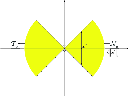
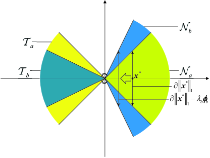
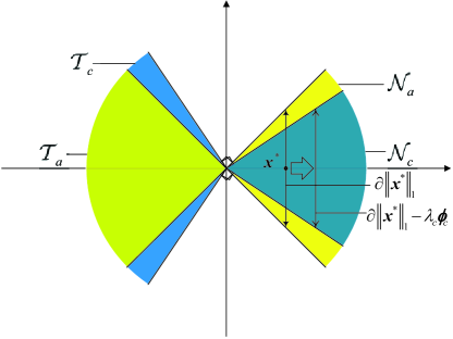
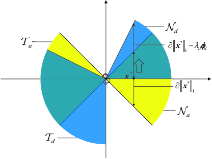
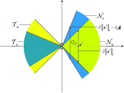
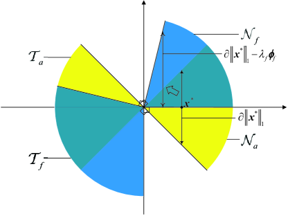
In what follows, we will illustrate these geometrical ideas by using two kinds of typical structured signals, namely, sparse vectors and low-rank matrices.

IV-A Geometrical Interpretation of Procedure (13)

For the sparse recovery procedure (13), recall that $I$ is the support of $\bm{x}^{\star}$. Since different shifts have different effects on the performance of (13), we define the following three kinds of shifts (or prior information), namely,

• a shift on $I$ if $\lambda\bm{\phi}$ satisfies

  $$\left\{{\begin{array}[]{ll}\lambda\bm{\phi}_{i}\neq 0,&\exists~{}i\in I,\\ \lambda\bm{\phi}_{i}=0,&\forall~{}i\in I^{c},\end{array}}\right.$$

• a shift on $I^{c}$ if $\lambda\bm{\phi}$ satisfies

  $$\left\{{\begin{array}[]{ll}\lambda\bm{\phi}_{i}=0,&\forall~{}i\in I,\\ \lambda\bm{\phi}_{i}\neq 0,&\exists~{}i\in I^{c},\end{array}}\right.$$

• an arbitrary shift if $\lambda\bm{\phi}$ satisfies

  $$\left\{{\begin{array}[]{ll}\lambda\bm{\phi}_{i}\neq 0,&\exists~{}i\in I,\\ \lambda\bm{\phi}_{i}\neq 0,&\exists~{}i\in I^{c}.\end{array}}\right.$$

For clarity, we consider a two dimensional example. We set $\bm{x}^{\star}=[1,0]^{T}$ and consider different prior information: $\lambda_{a}\bm{\phi}_{a}=\left[0,0\right]^{T},~{}\lambda_{b}\bm{\phi}_{b}=\left[0.5,0\right]^{T}~{}\lambda_{c}\bm{\phi}_{c}=\left[-0.5,0\right]^{T},~{}\lambda_{d}\bm{\phi}_{d}=\left[0,-1\right]^{T},~{}\lambda_{e}\bm{\phi}_{e}=\left[0.5,-0.2\right]^{T},$ and $\lambda_{f}\bm{\phi}_{f}=\left[0.5,-1\right]^{T}$. Fig. 1 illustrates the changes in geometry under different shifts.

TABLE I: $v_{1}$, $u_{1}$, upper bound I, upper bound II, and estimated Gaussian width under different shifts for sparse recovery.

Shift	$v_{1}$	$u_{1}$	bound I	bound II	Result
$\lambda_{a}\bm{\phi}_{a}$	2	1	1.68	2	1.68
$\lambda_{b}\bm{\phi}_{b}$	1.25	0.25	1.49	1.25	1.25
$\lambda_{c}\bm{\phi}_{c}$	3.25	2.25	1.80	3.25	1.80
$\lambda_{d}\bm{\phi}_{d}$	5	2	1.87	3	1.87
$\lambda_{e}\bm{\phi}_{e}$	1.69	0.29	1.62	1.29	1.29
$\lambda_{f}\bm{\phi}_{f}$	4.25	1.25	1.85	2.25	1.85

We draw Fig. 1(a) without shift for reference. The shifts in Fig. 1(b) and 1(c) are shifts on the support of $\bm{x}^{\star}$. In Fig. 1(b), the subdifferential moves toward the original, which enlarges the normal cone and hence decreases the number of measurements. The opposite result is shown in Fig. 1(c). The shift in Fig. 1(d) is a shift on the complement of the support of $\bm{x}^{\star}$, which leads to a growth of sample size because the normal cone is narrowed in this case. The shifts in Fig. 1(e) and 1(f) are arbitrary shifts. We can know from Fig. 1(e) and 1(f) that different arbitrary shifts may lead to different results: the number of measurements of Fig. 1(e) gets reduced while that of Fig. 1(f) gets increased.

(a) $\eta(\lambda_{a}\bm{\Phi}_{a})=\left[0,0,0\right]^{T}$

(b) $\eta(\lambda_{b}\bm{\Phi}_{b})=\left[0.25,0,0\right]^{T}$

(c) $\eta(\lambda_{c}\bm{\Phi}_{c})=\left[-0.25,0,0\right]^{T}$

(d) $\eta(\lambda_{d}\bm{\Phi}_{d})=\left[0,0,-0.5\right]^{T}$

(e) $\eta(\lambda_{e}\bm{\Phi}_{e})=\left[0.5,0,-0.2\right]^{T}$

(f) $\eta(\lambda_{f}\bm{\Phi}_{f})=\left[-0.25,0,-0.5\right]^{T}$

Figure 2: The changes of normal cone and tangent cone after different shifts for low-rank recovery. For reference, we draw the tangent cone $\mathcal{T}_{a}$ and normal come $\mathcal{N}_{a}$ for classical low-rank recovery in (a). In other subfigures, the tangent cones $\mathcal{T}_{\xi},~{}\xi=b,c,d,e,f$ and normal cones $\mathcal{N}_{\xi},~{}\xi=b,c,d,e,f$ are shown in blue for the approach (20) under different shifts. Good shifts, such as (b) and (e), enlarge the normal cone and hence decrease the number of measurements. Bad shifts, such as (c), (d), and (f), narrow the normal cone and lead to a growth of sample size.

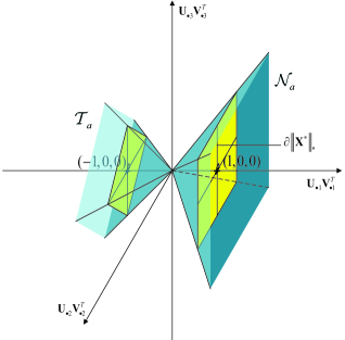
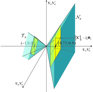
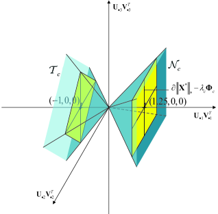
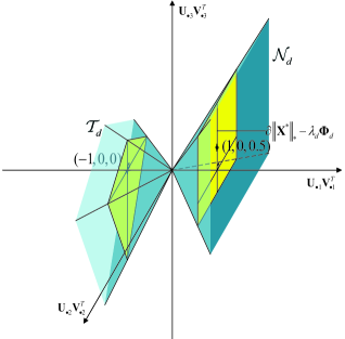
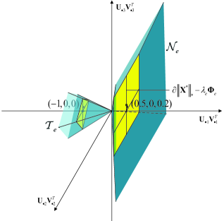
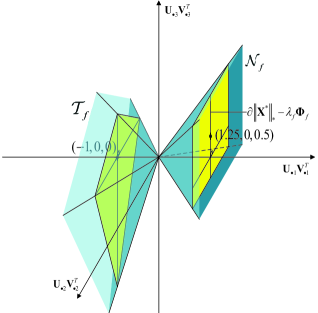
Table I lists related parameters ($v_{1}$ and $u_{1}$) and estimated Gaussian widths under different shifts. In each case, we calculate the two upper bounds in Lemma 1 and obtain the estimated Gaussian width by minimizing them. The results illustrate that the shifts $\lambda_{b}\bm{\phi}_{b}$ and $\lambda_{e}\bm{\phi}_{e}$ outperform the no shift case while the other shifts present an opposite result.

Therefore, we might conclude that with proper shifts, our approach can outperform BP.

IV-B Geometrical Interpretation of Procedure (20)

For low-rank matrix recovery procedure (20), recall that $\mathcal{S}$ is the space of matrices in the column or row space of $\bm{X}^{\star}$. We similarly consider three different kinds of shifts (or prior information), namely,

• a shift on $\mathcal{S}$ if $\bm{\Phi}$ satisfies

  $$\left\{{\begin{array}[]{ll}\mathcal{P}_{\mathcal{S}}(\bm{\Phi})&\neq\bm{0},\\ \mathcal{P}_{\mathcal{S}^{\bot}}(\bm{\Phi})&=\bm{0},\end{array}}\right.$$

• a shift on $\mathcal{S}^{\bot}$ if $\bm{\Phi}$ satisfies

  $$\left\{{\begin{array}[]{ll}\mathcal{P}_{\mathcal{S}}(\bm{\Phi})&=\bm{0},\\ \mathcal{P}_{\mathcal{S}^{\bot}}(\bm{\Phi})&\neq\bm{0},\end{array}}\right.$$

• an arbitrary shift if $\bm{\Phi}$ satisfies

  $$\left\{{\begin{array}[]{ll}\mathcal{P}_{\mathcal{S}}(\bm{\Phi})&\neq\bm{0},\\ \mathcal{P}_{\mathcal{S}^{\bot}}(\bm{\Phi})&\neq\bm{0}.\end{array}}\right.$$

For clarity, we consider a three dimensional example. Let

$$\bm{X}^{\star}=\bm{U}\left[\begin{array}[]{ccc}1&0&0\\ 0&0&0\\ 0&0&0\\ \end{array}\right]\bm{V}^{T},$$

be the SVD of $\bm{X}^{\star}$, and let $\bm{\Phi}=\sum_{k=1}^{3}[\eta(\bm{\Phi})]_{k}\bm{U}_{\cdot k}\bm{V}_{\cdot k}^{T}$ with $\eta(\bm{\Phi})\in\mathbb{R}^{3}$. We consider different prior information: $\eta(\lambda_{a}\bm{\Phi}_{a})=\left[0,0,0\right]^{T},~{}\eta(\lambda_{b}\bm{\Phi}_{b})=\left[0.25,0,0\right]^{T},~{}\eta(\lambda_{c}\bm{\Phi}_{c})=\left[-0.25,0,0\right]^{T},~{}\eta(\lambda_{d}\bm{\Phi}_{d})=\left[0,0,-0.5\right]^{T},~{}\eta(\lambda_{e}\bm{\Phi}_{e})=[0.5,0,-0.2]^{T}$, and $\eta(\lambda_{f}\bm{\Phi}_{f})=\left[-0.25,0,-0.5\right]^{T}$. It is not hard to check that $\lambda_{b}\bm{\Phi}_{b}$ and $\lambda_{c}\bm{\Phi}_{c}$ are shifts on $\mathcal{S}$, $\lambda_{d}\bm{\Phi}_{d}$ is a shift on $\mathcal{S}^{\perp}$, and $\lambda_{e}\bm{\Phi}_{e}$ and $\lambda_{f}\bm{\Phi}_{f}$ are arbitrary shifts. The changes in geometry under different shifts are shown in Fig. 2.

For reference, we draw Fig. 2(a) for the standard low-rank recovery procedure. Compared with Fig. 2(a), the shifts in Fig. 2(b) and 2(e) move toward the original, which enlarges the normal cone and hence decreases the number of measurements. On the contrary, the shifts in Fig. 2(c), 2(d), and 2(f) narrow the normal cone and hence lead to a growth of the sample size.

The related parameters ($v_{3}$ and $u_{3}$) and estimated Gaussian widths in Lemma 2 are shown in Table II. The results illustrate that the shifts $\lambda_{b}\bm{\Phi}_{b}$ and $\lambda_{e}\bm{\Phi}_{e}$ outperform the no shift case while the other shifts present an opposite result. Thus we may similarly conclude that with proper prior information, the procedure (20) can improve the performance of the standard recovery method.

TABLE II: $v_{3}$, $u_{3}$, upper bound I, upper bound II, and estimated Gaussian width under different shifts for low-rank matrix recovery.

Shift	$v_{3}$	$u_{3}$	bound I	bound II	Result
$\lambda_{a}\bm{\Phi}_{a}$	3	1	8.9707	15	8.9707
$\lambda_{b}\bm{\Phi}_{b}$	2.5625	0.5625	8.9657	10.625	8.9657
$\lambda_{c}\bm{\Phi}_{c}$	3.5625	1.5625	8.9754	20.625	8.9754
$\lambda_{d}\bm{\Phi}_{d}$	4.25	1.25	8.9793	17.5	8.9793
$\lambda_{e}\bm{\Phi}_{e}$	2.69	0.29	8.9674	7.9	7.9
$\lambda_{f}\bm{\Phi}_{f}$	4.8125	1.8125	8.9818	23.125	8.9818

IV-C Guidance for Improving Prior Information

The proofs of Theorems 2-4 have revealed that $v_{i}$ and $u_{i}$ ($i=1,2,3$) play a key role in evaluating the performance of our recovery procedures. More precisely, the less $v_{i}$ and $u_{i}$, the better the recovery performance. Therefore, these parameters might provide practical guidance to improve the quality of prior information.

Sparse recovery. In this case,

$$v_{1}=\sum\limits_{i\in I}(\operatorname{sign}(x_{i}^{\star})-\lambda\bm{\phi}_{i})^{2}+\sum\limits_{i\in I^{c}}(1+|\lambda\bm{\phi}_{i}|)^{2}$$ (24)

and

$$u_{1}=\sum\limits_{i\in I}(\operatorname{sign}(\bm{x}_{i}^{\star})-\lambda\bm{\phi}_{i})^{2}+\sum\limits_{i\in I^{c}}(\lambda\bm{\phi}_{i})^{2}.$$ (25)

It is not hard to find that

• For $i\in I^{c}$, $\bm{\phi}_{i}=0$ is preferred since $\sum_{i\in I^{c}}(1+|\lambda\bm{\phi}_{i}|)^{2}$ and $\sum_{i\in I^{c}}(\lambda\bm{\phi}_{i})^{2}$ cannot be less than that in the no shift case.

• For $i\in I$, $\sum_{i\in I}(\operatorname{sign}(\bm{x}_{i}^{\star})-\lambda\bm{\phi}_{i})^{2}$ may be smaller than that in the no shift case, provided that prior information is suitable, for example, $\lambda\bm{\phi}_{i}=\operatorname{sign}(\bm{x}_{i}^{\star})/2$ for $i\in I$.

These observations suggest the following strategies to reduce $v_{1}$ and $u_{1}$ and hence to improve the performance of (13)

• If the sparsity level $s$ of $\bm{x}^{\star}$ is known, then we can keep only top $s$ principal components of $\bm{\phi}$ (in terms of absolute values) and adjust the new shift as follows

  $$\tilde{\lambda}\tilde{\bm{\phi}}=\kappa\cdot\operatorname{sign}(\bm{\phi}_{T}),$$

  where $T$ is the support of $s$ principal components of $\bm{\phi}$ and $\kappa\in(0,1)$ is an adjustable parameter.

• If the sparsity level $s$ of $\bm{x}^{\star}$ is unknown, then we might estimate the stable sparsity level first [31]

  $$s=\frac{\left\lVert\bm{\phi}\right\rVert_{1}^{2}}{\left\lVert\bm{\phi}\right\rVert_{2}^{2}}.$$

  Thus we can repeat the procedures in (S1) and obtain the new shift.

Block-sparse recovery. In this case, standard calculation leads to

$$v_{2}=\sum\limits_{b\in\mathcal{B}}\left\lVert\frac{\bm{x}_{V_{b}}^{\star}}{\left\lVert\bm{x}_{V_{b}}^{\star}\right\rVert_{2}}-\lambda\bm{\phi}_{V_{b}}\right\rVert_{2}^{2}\\ +\sum\limits_{b\notin\mathcal{B}}\left(1+\lambda\left\lVert\bm{\phi}_{V_{b}}\right\rVert_{2}\right)^{2}$$ (26)

and

$$u_{2}=\sum\limits_{b\in\mathcal{B}}\left\lVert\frac{\bm{x}_{V_{b}}^{\star}}{\left\lVert\bm{x}_{V_{b}}^{\star}\right\rVert_{2}}-\lambda\bm{\phi}_{V_{b}}\right\rVert_{2}^{2}+\sum\limits_{b\notin\mathcal{B}}\left\lVert\lambda\bm{\phi}_{V_{b}}\right\rVert_{2}^{2}.$$ (27)

Similarly, we can find that

• For $b\notin\mathcal{B}$, $\bm{\phi}_{V_{b}}=0$ is preferred because $\sum_{b\notin\mathcal{B}}\left(1+\lambda\left\lVert\bm{\phi}_{V_{b}}\right\rVert_{2}\right)^{2}$ and $\sum_{b\notin\mathcal{B}}\left\lVert\lambda\bm{\phi}_{V_{b}}\right\rVert_{2}^{2}$ cannot be less than that in the no shift case.

• For $b\in\mathcal{B}$, $\sum_{b\in\mathcal{B}}\|{\bm{x}_{V_{b}}^{\star}}/{\|\bm{x}_{V_{b}}^{\star}\|_{2}}-\lambda\bm{\phi}_{V_{b}}\|_{2}^{2}$ may be less than that in the no shift case, provided that prior information is proper, for example, $\lambda\bm{\phi}=\frac{1}{2}\sum_{b\in\mathcal{B}}{\bm{x}_{V_{b}}^{\star}}/\left\lVert\bm{x}_{V_{b}}^{\star}\right\rVert_{2}$.

Thus we can reduce $v_{2}$ and $u_{2}$ by the following strategies

• If the number of non-zero blocks $l$ of $\bm{x}^{\star}$ is known, then we can keep only top $l$ principal blocks of $\bm{\phi}$ (in terms of the $\ell_{2}$-norm of the blocks) and obtain the new shift

  $$\tilde{\lambda}\tilde{\bm{\phi}}=\kappa\sum_{b\in\tilde{\mathcal{B}}}\frac{\bm{x}_{V_{b}}^{\star}}{\left\lVert\bm{x}_{V_{b}}^{\star}\right\rVert_{2}},$$

  where $\tilde{\mathcal{B}}$ is the support of principal blocks of $\bm{\phi}$ and $\kappa\in(0,1)$.

• If the number of non-zero blocks $l$ of $\bm{x}^{\star}$ is unknown, then we estimate the stable number of blocks as in [31]

  $$l=\frac{\left\lVert\bm{\phi}\right\rVert_{2,1}^{2}}{\left\lVert\bm{\phi}\right\rVert_{2}^{2}}.$$

  Thus, the new shift is gotten by repeating the procedures in (B1).

Low-rank recovery. In the low-rank matrix recovery case, direct calculation yields

$$v_{3}=\left\lVert\bm{U}\bm{V}^{T}-\lambda\mathcal{P}_{\mathcal{S}}(\bm{\Phi})\right\rVert_{F}^{2}+\max\limits_{\bm{W}\in\mathcal{S}^{\bot},\left\lVert\bm{W}\right\rVert\leq 1}\left\lVert\bm{W}-\lambda\mathcal{P}_{\mathcal{S}^{\bot}}(\bm{\Phi})\right\rVert_{F}^{2},$$ (28)

and

$$u_{3}=\left\lVert\bm{U}\bm{V}^{T}-\lambda\mathcal{P}_{\mathcal{S}}(\bm{\Phi})\right\rVert_{F}^{2}+\left\lVert\lambda\mathcal{P}_{\mathcal{S}^{\bot}}(\bm{\Phi})\right\rVert_{F}^{2}.$$ (29)

From the above expressions, it is not hard to see that the left and right singular vectors of non-zero singular values of $\bm{\Phi}$ play a critical role in improving the quantity of priori information. Let $\bm{\Phi}=\hat{\bm{U}}\hat{\bm{\Sigma}}\hat{\bm{V}}$ be the SVD of $\bm{\Phi}$, then we can similarly obtain the following strategies

• If the rank $r$ of $\bm{X}^{\star}$ is known, then we improve the new shift as follows

  $$\tilde{\lambda}\tilde{\bm{\Phi}}=\kappa\cdot\hat{\bm{U}}_{r}\hat{\bm{V}}_{r}^{T},$$

  where $\hat{\bm{U}}_{r}$ and $\hat{\bm{V}}_{r}$ consist of the first $r$ left and right singular vectors of $\bm{\Phi}$ respectively and $\kappa\in(0,1)$.

• If the rank $r$ of $\bm{X}^{\star}$ is unknown, we should estimate the numerical rank first. For example, we can use the way in [32]

  $$r=\frac{\left\lVert\bm{\Phi}\right\rVert_{\text{F}}^{2}}{\left\lVert\bm{\Phi}\right\rVert^{2}}.$$

  Repeating the procedures in (L1) completes the new shift.

V Numerical Simulations

In this section, we carry out some numerical simulations to verify the correctness of our theoretical results.

V-A Phase Transition for Sparse Recovery

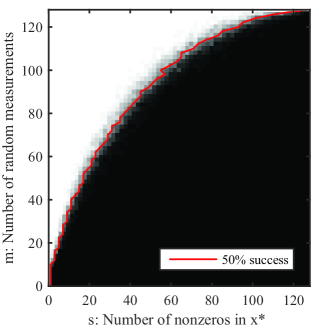
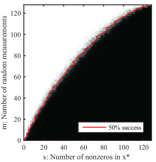
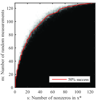
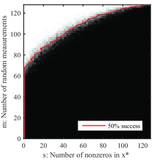
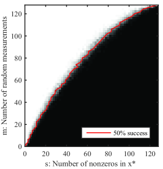
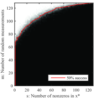
In this experiment, we draw some phase transition curves in the absence of noise for different kinds of prior information: no shift, shifts on the support, shifts on the complement of the support, and arbitrary shifts. The original signal $\bm{x}^{\star}\in\mathbb{R}^{n}$ is an $s$-sparse random vector whose nonzero entries are drawn from the standard Gaussian distribution and the measurement matrix $\bm{A}\in\mathbb{R}^{m\times n}$ is a Bernoulli matrix with i.i.d. entries obeying the symmetric Bernoulli distribution. We set $n=128$ and $tol=10^{-2}$ for all the experiments. For a particular pair of $s$ and $m$, we make 50 trials, count the number of trials which succeed to recover $\bm{x}^{\star}$, and calculate the related probability. Let $\hat{\bm{x}}$ be the solution of (13). If the solution of a trial satisfies

$$\frac{\left\lVert\bm{x}^{\star}-\hat{\bm{x}}\right\rVert_{2}}{\left\lVert\bm{x}^{\star}\right\rVert_{2}}<tol,$$

then we claim it as a successful trial. We increase both $m$ and $s$ from $0$ to $n$ with step $2$, then we can obtain a phase transition curve.

We consider six different shifts:

1. $\lambda\bm{\phi}=\bm{0}$. This is the classical CS model.

2. $\lambda\bm{\phi}=\text{sign}(\bm{x}^{\star})/2$. This is a shift on the support.

3. $\lambda\bm{\phi}=-\text{sign}(\bm{x}^{\star})/2$. This is a shift on the support.

4. $\lambda\bm{\phi}_{i}=0$ for $i\in I$ and $\lambda\bm{\phi}_{i}=1$ for $i\in I^{c}$. This is a shift on the complement of the support.

5. $\lambda\bm{\phi}_{i}=\text{sign}(\bm{x}^{\star}_{i})/2$ for $i\in I$ and $\lambda\bm{\phi}_{i}=0$ for $i\in I^{c}$ except an arbitrary $i\in I^{c}$ satisfying $\lambda\bm{\phi}_{i}=1/4$. This is an arbitrary shift.

6. $\lambda\bm{\phi}_{i}=-\text{sign}(\bm{x}^{\star}_{i})/2$ for $i\in I$ and $\lambda\bm{\phi}_{i}=1$ for $i\in I^{c}$. This is an arbitrary shift.

The results are shown in Fig 3. For shifts on the support, Fig. 3(b) shows an improved performance while Fig. 3(c) presents a deteriorative performance in contrast to the standard CS result in Fig. 3(a). Comparing Fig. 3(d) with Fig. 3(a), we realize that the shift on the complement of the support makes the number of measurements increase whatever the sparsity level is. In Fig. 3(e), the simulation result shows that this arbitrary shift improves the performance a lot compared with Fig. 3(a). However, Fig. 3(f) presents an opposite result for another arbitrary shift. All of these numerical results are consistent with our theoretical result (Theorem 2) and geometrical interpretation. From these results, we can conclude that if prior information is good enough, then our method can perform better than BP.

V-B Performance Comparisons with Other Approaches for Sparse Recovery

We next run some experiments to compare the performance of BP, $\ell_{1}$-$\ell_{1}$ minimization, $\ell_{1}$-$\ell_{2}$ minimization, the proposed method (denoted by maximizing correlation (MC)), improved MC with known sparsity, and improved MC with unknown sparsity. Here, two improved MCs follow the strategies in Section IV-C for sparse recovery.

(a) $\lambda\bm{\phi}=\bm{0}$

(b) $\lambda\bm{\phi}=\frac{\text{sign}(\bm{x}^{\star})}{2}$

(c) $\lambda\bm{\phi}=-\frac{\text{sign}(\bm{x}^{\star})}{2}$

(d) $\lambda\bm{\phi}_{i}=0$ for $i\in I$ and $\lambda\bm{\phi}_{i}=1$ for $i\in I^{c}$

(e) $\lambda\bm{\phi}_{i}=\text{sign}(\bm{x}^{\star}_{i})/2$ for $i\in I$ and $\lambda\bm{\phi}_{i}=0$ for $i\in I^{c}$ except an arbitrary $i\in I^{c}$ satisfying $\lambda\bm{\phi}_{i}=1/4$

(f) $\lambda\bm{\phi}_{i}=-\text{sign}(\bm{x}^{\star}_{i})/2$ for $i\in I$ and $\lambda\bm{\phi}_{i}=1$ for $i\in I^{c}$

Figure 3: The phase transition curves for different shifts. The brightness of each point reflects the observed probability of success, ranging from black (0%) to white (100%).

(a) $\bm{z}$: random sparse perturbation

(b) $\bm{z}$: random dense perturbation

Figure 4: Rate of successful reconstruction v.s. number of measurements under prior information $\bm{\phi}=\bm{x}^{\star}+\bm{z}$ for BP, $\ell_{1}$-$\ell_{1}$ minimization, $\ell_{1}$-$\ell_{2}$ minimization, maximizing correlation (MC), improved MC with known sparsity, and improved MC with unknown sparsity. (a) $\bm{z}$ is a random sparse perturbation. (b) $\bm{z}$ is a random dense perturbation.

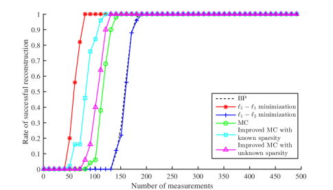
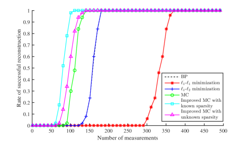
The original signal $\bm{x}^{\star}$ is a sparse vector with dimension $n=500$ and sparsity $s=50$. The nonzero entries of $\bm{x}^{\star}$ are drawn from the standard Gaussian distribution. The prior information is generated as $\bm{\phi}=\bm{x}^{\star}+\bm{z}$. We consider two kinds of perturbation vector $\bm{z}$:

• Random sparse perturbation. $\bm{z}$ is a $20$-sparse vector whose nonzero entries are drawn from a zero-mean Gaussian random variable with standard deviation $0.5$. The supports of $\bm{x}^{\star}$ and $\bm{z}$ coincide in $16$ positions and differ in $4$ positions.

• Random dense perturbation. The entries of $\bm{z}$ are drawn from a zero-mean Gaussian variable with standard deviation $0.1$.

The measurement matrix $\bm{A}\in\mathbb{R}^{m\times n}$ is a Bernoulli matrix. The observation noise $\bm{n}\in\mathbb{R}^{m}$ is a random vector whose entries are independently drawn from a zero-mean Gaussian distribution with standard deviation $0.01$. We set the upper bound of the noise vector $\delta=\left\lVert\bm{n}\right\rVert_{2}$. For a fixed number of measurements $m$, we make $50$ trials, and calculate the successful probability as before. We set $\lambda=1$ for $\ell_{1}$-$\ell_{1}$ minimization, $\ell_{1}$-$\ell_{2}$ minimization and MC, and set $\kappa=0.95$ for two improved MCs.

The results under random sparse perturbation are shown in Fig. 4(a). The figure shows that $\ell_{1}$-$\ell_{1}$ minimization performs the best. This is because $\bm{\phi}-\bm{x}^{\star}$ is a sparse vector in this case and the $\ell_{1}$-norm is effective to promote sparsity. We also find that all three MCs outperform BP and $\ell_{1}$-$\ell_{2}$ minimization. In addition, the results indicates that the strategies for improving prior information are effective since the two improved MCs show a better performance than the normal one. The plot also illustrates that the improved MC with known sparsity outperforms the one with unknown sparsity.

Fig. 4(b) shows the experiment results under random dense perturbation. The plot shows that all three MCs perform better than the other methods. $\ell_{1}$-$\ell_{1}$ minimization performs the worst in this case since $\bm{\phi}-\bm{x}^{\star}$ is not a sparse vector anymore. BP and $\ell_{1}$-$\ell_{2}$ minimization almost coincide everywhere. For three MCs, a similar phenomenon is observed that the two improved MCs have a better performance than the normal one and that the improved MC with known sparsity outperforms the one with unknown sparsity.

In conclusion, whether the perturbation is sparse or dense, the proposed method can have a relatively good performance. Furthermore, the simulations validate the effectiveness of the proposed guidance for improving prior information.

V-C Phase Transition for Low-rank Recovery

For low-rank matrix recovery, we also draw some phase transition curves in the absence of noise for different kinds of prior information: no shift, shifts on $\mathcal{S}$, shifts on $\mathcal{S}^{\perp}$, and arbitrary shifts. Let $\bm{X}\in\mathbb{R}^{n\times n}$ be a Gaussian matrix with i.i.d. entries satisfying the standard Gaussian distribution. Let $\bm{X}=\tilde{\bm{U}}\tilde{\bm{\Sigma}}\tilde{\bm{V}}^{T}=\sum_{k=1}^{n}\tilde{\sigma}_{k}\tilde{\bm{U}}_{\cdot k}\tilde{\bm{V}}_{\cdot k}^{T}$ be the SVD of $\bm{X}$. The original signal $\bm{X}^{\star}=\sum_{k=1}^{r}\tilde{\sigma}_{k}\tilde{\bm{U}}_{\cdot k}\tilde{\bm{V}}_{\cdot k}^{T}\in\mathbb{R}^{n\times n}$ is a rank-$r$ matrix and the measurement matrices $\{\bm{A}^{j}\}_{j=1}^{m}$ are independent Bernoulli matrices. We set $n=32$ and $tol=10^{-2}$ for all the experiments. For a particular pair of $r$ and $m$, we make 50 trials, count the number of trials which succeed to recover $\bm{X}^{\star}$, and calculate the related probability. If the solution of a trial satisfies

$$\frac{\left\lVert\bm{X}^{\star}-\hat{\bm{X}}\right\rVert_{\text{F}}}{\left\lVert\bm{X}^{\star}\right\rVert_{\text{F}}}<tol,$$

we claim it as a successful trial. Let $r$ increase from $0$ to $n$ with step 1 and $m$ increase from $0$ to $n^{2}$ with step $n$, then we can obtain a phase transition curve.

We consider six different shifts:

1. $\lambda\bm{\Phi}=\bm{0}$. This is the classical CS model for low-rank recovery.

2. $\lambda\bm{\Phi}=\bm{U}\bm{V}^{T}/2$. This is a shift on $\mathcal{S}$.

3. $\lambda\bm{\Phi}=-\bm{U}\bm{V}^{T}/2$. This is a shift on $\mathcal{S}$.

4. $\lambda\bm{\Phi}=\bm{U}^{\prime}\bm{V}^{\prime T}/2$. This is a shift on $\mathcal{S}^{\perp}$.

5. $\lambda\bm{\Phi}=\bm{U}\bm{V}^{T}/2+\bm{U}^{\prime}\operatorname*{diag}(1/2,0,\ldots,0)\bm{V}^{\prime T}$. This is an arbitrary shift.

6. $\lambda\bm{\Phi}=-\bm{U}\bm{V}^{T}/2+\bm{U}^{\prime}\bm{V}^{\prime T}/2$. This is an arbitrary shift.

(a) $\lambda\bm{\Phi}=\bm{0}$

(b) $\lambda\bm{\Phi}=\bm{U}\bm{V}^{T}/2$

(c) $\lambda\bm{\Phi}=-\bm{U}\bm{V}^{T}/2$

(d) $\lambda\bm{\Phi}=\bm{U}^{\prime}\bm{V}^{\prime T}/2$

(e) $\lambda\bm{\Phi}=\bm{U}\bm{V}^{T}/2+\bm{U}^{\prime}\operatorname*{diag}(1/2,0,\ldots,0)\bm{V}^{\prime T}$

(f) $\lambda\bm{\Phi}=-\bm{U}\bm{V}^{T}/2+\bm{U}^{\prime}\bm{V}^{\prime T}/2$

Figure 5: The phase transition curves of low-rank recovery under different shifts . The brightness of each point reflects the observed probability of success, ranging from black (0%) to white (100%).

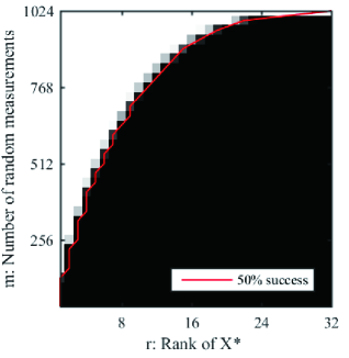
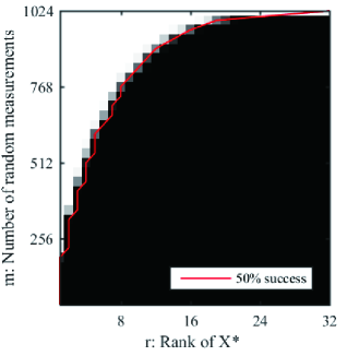
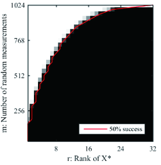
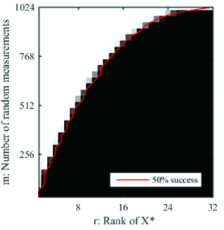
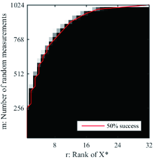
For reference, we draw Fig. 5(a) for the classical low-rank recovery procedure without prior information. For shifts on $\mathcal{S}$, Fig. 5(b) improves the performance a lot while Fig. 5(c) deteriorates the performance compared to Fig. 5(a). Comparing Fig. 5(d) with Fig. 5(a), we realize that the shift on $\mathcal{S}^{\perp}$ increases the number of measurements. Fig. 5(e) shows an improved performance for this arbitrary shift. However, Fig. 5(f) presents an opposite result for another arbitrary shift. All of these experimental results coincide with our theoretical result (Theorem 4) and geometrical interpretation. From these results, we also come to the conclusion that with proper prior information, our approach can have a better performance than the classical low-rank recovery procedure.

Figure 6: Rate of successful reconstruction v.s. number of measurements for the standard low-rank recovery procedure, MC, improved MC with known rank, and improved MC with unknown rank.

V-D Performance Comparisons with Standard Approach for Low-rank Recovery

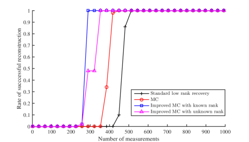
In this experiment, we compare the performance of the standard low-rank recovery procedure, MC (20), improved MC with known rank, and improved MC with unknown rank. Here, improved MCs follow the strategies in Section IV-C for low-rank matrix recovery.

The original signal $\bm{X}^{\star}\in\mathbb{R}^{n\times n}$ is generated similarly as in the previous subsection and the measurement matrices $\{\bm{A}^{j}\}_{j=1}^{m}$ are independent Bernoulli matrices. The observation noise $\bm{n}\in\mathbb{R}^{m}$ is a random vector whose entries are independently drawn from a zero-mean Gaussian distribution with standard deviation $0.01$. We set the upper bound of the noise vector $\delta=\left\lVert\bm{n}\right\rVert_{2}$. The prior information is generated as $\bm{\Phi}=\bm{X}^{\star}+\bm{Z}$, where the entries of $\bm{Z}$ are drawn from a zero-mean Gaussian distribution with standard deviation $0.1$. We set $n=32$ and $r=5$. For a fixed $m$, we make $50$ trials and calculate the successful probability as before. We set $\lambda=1/n$ for MC and $\kappa=0.95$ for two improved MCs. The results are shown in Fig. 6.

Compared to the standard low-rank recovery procedure, all three MCs require less measurements to reconstruct $\bm{X}^{\star}$ successfully. For the MC approaches, the two improved MCs outperform the normal one and the improved MC with known rank shows a better performance than the one with unknown rank. In summary, our approach can improve the performance of the standard low-rank recovery procedure. The simulation results also illustrate the validity of the guidance for improving prior information.

VI Conclusion

This paper has proposed a new approach to recover structured signals with the aid of a similar signal which is known a priori. Theoretical bounds on the number of measurements have been established under sub-Gaussian measurements. Specific structured signals including sparse vectors, block-sparse vectors, and low-rank matrices has also been analyzed. The corresponding geometrical interpretation has been given to illustrate the essence of the proposed approach. Our theoretical results and geometrical interpretation also suggest some strategies to improve the quality of prior information. Numerical simulations are provided to demonstrate the validity of the results.

Appendix A

A-A Proof of Lemma 1

According to Fact 2, we have

$$w(\mathcal{T}_{f}\cap\mathbb{S}^{n-1})\leq\operatorname{\mathbb{E}}[\operatorname{dist}(\bm{g},\mathcal{N}_{f})],$$

where $\mathcal{N}_{f}$ denotes the polar of $\mathcal{T}_{f}$. Since $\bm{0}\notin\partial\left\lVert\bm{x}^{\star}\right\rVert_{1}-\lambda\bm{\phi}$, it then follows from Fact 1 that

$$\mathcal{N}_{f}=\text{cone}\{\partial\left\lVert\bm{x}^{\star}\right\rVert_{1}-\lambda\bm{\phi}\}.$$

Thus, by Jensen’s inequality, we have

$$w^{2}(\mathcal{T}_{f}\cap\mathbb{S}^{n-1})\leq\operatorname{\mathbb{E}}[\operatorname{dist}^{2}(\bm{g},\text{cone}\{\partial\left\lVert\bm{x}^{\star}\right\rVert_{1}-\lambda\bm{\phi}\})].$$ (30)

Upper bound I. Fix any $\bm{g}\in\mathbb{R}^{n}$ and choose any

$$\bm{w}_{0}\in\arg\max\limits_{\bm{w}\in\partial\left\lVert\bm{x}^{\star}\right\rVert_{1}-\lambda\bm{\phi}}\left\langle\bm{g},\bm{w}\right\rangle,$$

then we have, for any $t\geq 0$,

$$\operatorname{dist}^{2}(\bm{g},\text{\emph{cone}}\{\partial\left\lVert\bm{x}^{\star}\right\rVert_{1}-\lambda\bm{\phi}\}) \leq\operatorname{dist}^{2}(\bm{g},t\cdot(\partial\left\lVert\bm{x}^{\star}\right\rVert_{1}-\lambda\bm{\phi}))$$

$$\leq\left\lVert\bm{g}-t\bm{w}_{0}\right\rVert_{2}^{2}=\left\lVert\bm{g}\right\rVert_{2}^{2}-2t\left\langle\bm{g},\bm{w}_{0}\right\rangle+t^{2}\left\lVert\bm{w}_{0}\right\rVert_{2}^{2}$$

$$=\left\lVert\bm{g}\right\rVert_{2}^{2}-2t\max\limits_{\bm{w}\in\partial\left\lVert\bm{x}^{\star}\right\rVert_{1}-\lambda\bm{\phi}}\left\langle\bm{g},\bm{w}\right\rangle+t^{2}\left\lVert\bm{w}_{0}\right\rVert_{2}^{2}$$

$$\leq\left\lVert\bm{g}\right\rVert_{2}^{2}-2t\max\limits_{\bm{w}\in\partial\left\lVert\bm{x}^{\star}\right\rVert_{1}-\lambda\bm{\phi}}\left\langle\bm{g},\bm{w}\right\rangle+t^{2}\max\limits_{\bm{w}\in\partial\left\lVert\bm{x}^{\star}\right\rVert_{1}-\lambda\bm{\phi}}\left\lVert\bm{w}\right\rVert_{2}^{2}.$$

Taking expectation on both sides yields

$$\operatorname{\mathbb{E}}\left[\operatorname{dist}^{2}(\bm{g},t\cdot(\partial\left\lVert\bm{x}^{\star}\right\rVert_{1}-\lambda\bm{\phi}))\right] \leq n-2t\cdot\operatorname{\mathbb{E}}\max\limits_{\bm{w}\in\partial\left\lVert\bm{x}^{\star}\right\rVert_{1}-\lambda\bm{\phi}}\left\langle\bm{g},\bm{w}\right\rangle+t^{2}\cdot\max\limits_{\bm{w}\in\partial\left\lVert\bm{x}^{\star}\right\rVert_{1}-\lambda\bm{\phi}}\left\lVert\bm{w}\right\rVert_{2}^{2}$$ (31)

$$=n-2t\cdot\sqrt{\frac{2}{\pi}}(n-s)+t^{2}\cdot v_{1},$$

where

$$\operatorname{\mathbb{E}}\max\limits_{\bm{w}\in\partial\left\lVert\bm{x}^{\star}\right\rVert_{1}-\lambda\bm{\phi}}\left\langle\bm{g},\bm{w}\right\rangle=\operatorname{\mathbb{E}}\max\limits_{\bm{w}\in\partial\left\lVert\bm{x}^{\star}\right\rVert_{1}}\left\langle\bm{g},\bm{w}\right\rangle=\sqrt{\frac{2}{\pi}}(n-s).$$

Choosing $t=\sqrt{2/\pi}(n-s)/v_{1}$, we achieve the minimum of (31) and get the first upper bound.

Upper bound II. Define

$$z(\bm{g}):=\left\lVert\bm{g}_{I^{c}}\right\rVert_{2}\cdot\left(\operatorname{sign}(\bm{x}^{\star})+\frac{\bm{g}_{I^{c}}}{\left\lVert\bm{g}_{I^{c}}\right\rVert_{2}}-\lambda\bm{\phi}\right)=\left\lVert\bm{g}_{I^{c}}\right\rVert_{2}(\operatorname{sign}(\bm{x}^{\star})-\lambda\bm{\phi})+\bm{g}_{I^{c}}.$$

Since $\left\{\operatorname{sign}(\bm{x}^{\star})+\bm{g}_{I^{c}}/\left\lVert\bm{g}_{I^{c}}\right\rVert_{2}\right\}\in\partial\left\lVert\bm{x}^{\star}\right\rVert_{1}$, we have $z(\bm{g})\in\text{cone}\{\partial\left\lVert\bm{x}^{\star}\right\rVert_{1}-\lambda\bm{\phi}\}$ and

$$\operatorname{\mathbb{E}}\left[\operatorname{dist}^{2}(\bm{g},\text{cone}\{\partial\left\lVert\bm{x}^{\star}\right\rVert_{1}-\lambda\bm{\phi}\})\right] \leq\operatorname{\mathbb{E}}\left\lVert\bm{g}-z(\bm{g})\right\rVert_{2}^{2}$$

$$=\operatorname{\mathbb{E}}\left\lVert\bm{g}_{I}-\left\lVert\bm{g}_{I^{c}}\right\rVert_{2}\left(\operatorname{sign}(\bm{x}^{\star})-\lambda\bm{\phi}\right)\right\rVert_{2}^{2}$$

$$=\operatorname{\mathbb{E}}\left\lVert\bm{g}_{I}\right\rVert_{2}^{2}+\left\lVert\operatorname{sign}(\bm{x}^{\star})-\lambda\bm{\phi}\right\rVert_{2}^{2}\operatorname{\mathbb{E}}\left\lVert\bm{g}_{I^{c}}\right\rVert_{2}^{2}$$ (32)

$$=s+(n-s)u_{1}.$$ (33)

Here (32) holds because $\bm{g}_{I}$ and $\bm{g}_{I^{c}}$ are independent. (33) follows because $\operatorname{\mathbb{E}}\left\lVert\bm{g}_{I}\right\rVert_{2}^{2}=s$ and $\operatorname{\mathbb{E}}\left\lVert\bm{g}_{I^{c}}\right\rVert_{2}^{2}=n-s$.

Minimizing the two upper bounds completes the proof.

A-B Proof of Lemma 2

According to Facts 1 and 2, for any $t\geq 0$ and $\bm{0}\notin\partial\left\lVert\bm{x}^{\star}\right\rVert_{2,1}-\lambda\bm{\phi}$, we have

$$w^{2}(\mathcal{T}_{f}\cap\mathbb{S}^{n-1}) \leq\operatorname{\mathbb{E}}\left[\operatorname{dist}^{2}(\bm{g},\mathcal{N}_{f})\right]$$

$$\leq\operatorname{\mathbb{E}}\left[\operatorname{dist}^{2}(\bm{g},t\cdot(\partial\left\lVert\bm{x}^{\star}\right\rVert_{2,1}-\lambda\bm{\phi}))\right],$$

where $\mathcal{N}_{f}=\text{cone}\{\partial\left\lVert\bm{x}^{\star}\right\rVert_{2,1}-\lambda\bm{\phi}\}$.

Upper bound I. Fix any $\bm{g}\in\mathbb{R}^{n}$ and choose any

$$\bm{w}_{0}\in\arg\max\limits_{\bm{w}\in\partial\left\lVert\bm{x}^{\star}\right\rVert_{2,1}-\lambda\bm{\phi}}\left\langle\bm{g},\bm{w}\right\rangle,$$

then we obtain

$$\operatorname{dist}^{2}(\bm{g},t\cdot(\partial\left\lVert\bm{x}^{\star}\right\rVert_{2,1}-\lambda\bm{\phi})) \leq\left\lVert\bm{g}-t\bm{w}_{0}\right\rVert_{2}^{2}=\left\lVert\bm{g}\right\rVert_{2}^{2}-2t\left\langle\bm{g},\bm{w}_{0}\right\rangle+t^{2}\left\lVert\bm{w}_{0}\right\rVert_{2}^{2}$$

$$=\left\lVert\bm{g}\right\rVert_{2}^{2}-2t\max\limits_{\bm{w}\in\partial\left\lVert\bm{x}^{\star}\right\rVert_{2,1}-\lambda\bm{\phi}}\left\langle\bm{g},\bm{w}\right\rangle+t^{2}\left\lVert\bm{w}_{0}\right\rVert_{2}^{2}$$

$$\leq\left\lVert\bm{g}\right\rVert_{2}^{2}-2t\max\limits_{\bm{w}\in\partial\left\lVert\bm{x}^{\star}\right\rVert_{2,1}-\lambda\bm{\phi}}\left\langle\bm{g},\bm{w}\right\rangle+t^{2}v_{2}.$$

Taking expectation on both sides yields

$$\operatorname{\mathbb{E}}\left[\operatorname{dist}^{2}(\bm{g},t\cdot(\partial\left\lVert\bm{x}^{\star}\right\rVert_{2,1}-\lambda\bm{\phi}))\right] \leq n-2t\operatorname{\mathbb{E}}\max\limits_{\bm{w}\in\partial\left\lVert\bm{x}^{\star}\right\rVert_{2,1}-\lambda\bm{\phi}}\left\langle\bm{g},\bm{w}\right\rangle+t^{2}v_{2}$$

$$=n-2tw(\partial\left\lVert\bm{x}^{\star}\right\rVert_{2,1})+t^{2}v_{2},$$ (34)

where $\operatorname{\mathbb{E}}\left\lVert\bm{g}\right\rVert_{2}^{2}=n$ and

$$\operatorname{\mathbb{E}}\max\limits_{\bm{w}\in\partial\left\lVert\bm{x}^{\star}\right\rVert_{2,1}-\lambda\bm{\phi}}\left\langle\bm{g},\bm{w}\right\rangle=w(\partial\left\lVert\bm{x}^{\star}\right\rVert_{2,1}).$$

By the subdifferential of the $\ell_{1}/\ell_{2}$-norm, we

$$w\left(\partial\left\lVert\bm{x}^{\star}\right\rVert_{2,1}\right) =\operatorname{\mathbb{E}}\max\limits_{\bm{w}\in\partial\left\lVert\bm{x}^{\star}\right\rVert_{2,1}}\left\langle\bm{g},\bm{w}\right\rangle$$

$$=\operatorname{\mathbb{E}}\left[\sum\limits_{b\in\mathcal{B}}\left\langle\bm{g}_{V_{b}},\frac{\bm{x}^{\star}_{V_{b}}}{\left\lVert\bm{x}^{\star}_{V_{b}}\right\rVert_{2}}\right\rangle+\sum\limits_{b\notin\mathcal{B}}\max\limits_{\left\lVert\bm{\theta}_{V_{b}}\right\rVert_{2}\leq 1}\left\langle\bm{g}_{V_{b}},\bm{\theta}_{V_{b}}\right\rangle\right]$$

$$=\sum\limits_{b\notin\mathcal{B}}\operatorname{\mathbb{E}}\max\limits_{\left\lVert\bm{\theta}_{V_{b}}\right\rVert_{2}\leq 1}\left\langle\bm{g}_{V_{b}},\bm{\theta}_{V_{b}}\right\rangle=\sum\limits_{b\notin\mathcal{B}}\operatorname{\mathbb{E}}\left\lVert\bm{g}_{V_{b}}\right\rVert_{2}$$

$$=(l-s)\mu_{k}.$$ (35)

Combining (A-B) and (A-B), we can achieve the minimum at $t=(l-s)\mu_{k}/v_{2}$ and get the first upper bound.

Upper bound II. Define

$$z(\bm{g})=\left\lVert\sum\limits_{b\notin\mathcal{B}}\bm{g}_{V_{b}}\right\rVert_{2}\left(\sum_{b\in\mathcal{B}}\frac{\bm{x}_{V_{b}}^{\star}}{\left\lVert\bm{x}_{V_{b}}^{\star}\right\rVert_{2}}+\frac{\sum_{b\notin\mathcal{B}}\bm{g}_{V_{b}}}{\left\lVert\sum_{b\notin\mathcal{B}}\bm{g}_{V_{b}}\right\rVert_{2}}-\lambda\bm{\phi}\right)=\left\lVert\sum\limits_{b\notin\mathcal{B}}\bm{g}_{V_{b}}\right\rVert_{2}\left(\sum_{b\in\mathcal{B}}\frac{\bm{x}_{V_{b}}^{\star}}{\left\lVert\bm{x}_{V_{b}}^{\star}\right\rVert_{2}}-\lambda\bm{\phi}\right)+\sum_{b\notin\mathcal{B}}\bm{g}_{V_{b}}.$$

Since

$$\sum_{b\in\mathcal{B}}\frac{\bm{x}_{V_{b}}^{\star}}{\left\lVert\bm{x}_{V_{b}}^{\star}\right\rVert_{2}}+\frac{\sum_{b\notin\mathcal{B}}\bm{g}_{V_{b}}}{\left\lVert\sum_{b\notin\mathcal{B}}\bm{g}_{V_{b}}\right\rVert_{2}}\in\partial\left\lVert\bm{x}^{\star}\right\rVert_{2,1},$$

we have $z(\bm{g})\in\text{cone}\{\partial\left\lVert\bm{x}^{\star}\right\rVert_{2,1}-\lambda\bm{\phi}\}$. Then

$$\operatorname{\mathbb{E}}\left[\operatorname{dist}^{2}(\bm{g},\text{cone}\{\partial\left\lVert\bm{x}^{\star}\right\rVert_{2,1}-\lambda\bm{\phi}\})\right] \leq\operatorname{\mathbb{E}}\left\lVert\bm{g}-z(\bm{g})\right\rVert_{2}^{2}$$

$$=\operatorname{\mathbb{E}}\left\lVert\sum_{b\in\mathcal{B}}\bm{g}_{V_{b}}-\left\lVert\sum\limits_{b\notin\mathcal{B}}\bm{g}_{V_{b}}\right\rVert_{2}\left(\sum_{b\in\mathcal{B}}\frac{\bm{x}_{V_{b}}^{\star}}{\left\lVert\bm{x}_{V_{b}}^{\star}\right\rVert_{2}}-\lambda\bm{\phi}\right)\right\rVert_{2}^{2}$$

$$=\sum_{b\in\mathcal{B}}\operatorname{\mathbb{E}}\left\lVert\bm{g}_{V_{b}}\right\rVert_{2}^{2}+u_{2}\cdot\left(\sum\limits_{b\notin\mathcal{B}}\operatorname{\mathbb{E}}\left\lVert\bm{g}_{V_{b}}\right\rVert_{2}^{2}\right)$$ (36)

$$=k\cdot\left(s+(l-s)u_{2}\right).$$ (37)

Here (36) holds because $\sum_{b\in\mathcal{B}}\bm{g}_{V_{b}}$and $\sum_{b\notin\mathcal{B}}\bm{g}_{V_{b}}$ are independent. (37) follows from $\operatorname{\mathbb{E}}\left\lVert\bm{g}_{V_{b}}\right\rVert_{2}^{2}=k,\forall~{}b\in\mathcal{B}$.

Minimizing the two upper bounds completes the proof.

A-C Proof of Lemma 3

Let $\bm{G}\in\mathbb{R}^{n_{1}\times n_{2}}$ be a Gaussian random matrix with i.i.d. standard Gaussian entries. According to Facts 1 and 2, if $\bm{0}\notin\partial\left\lVert\bm{X}^{\star}\right\rVert_{*}-\lambda\bm{\Phi}$, then for any $t\geq 0$,

$$w^{2}(\mathcal{T}_{f}\cap\mathbb{S}^{n_{1}n_{2}-1})\leq\operatorname{\mathbb{E}}[\operatorname{dist}^{2}(\bm{G},\text{cone}\{\partial\left\lVert\bm{X}^{\star}\right\rVert_{*}-\lambda\bm{\Phi}\})]\leq\operatorname{\mathbb{E}}[\operatorname{dist}^{2}(\bm{G},t\cdot(\partial\left\lVert\bm{X}^{\star}\right\rVert_{*}-\lambda\bm{\Phi}))],$$

where $\operatorname{dist}^{2}(\bm{X},\bm{Y})=\left\lVert\bm{X}-\bm{Y}\right\rVert_{F}^{2}$.

Upper bound I. Fix any $\bm{G}\in\mathbb{R}^{n_{1}\times n_{2}}$ and choose any

$$\bm{Z}_{0}\in\arg\max\limits_{\bm{Z}\in\partial\left\lVert\bm{X}^{\star}\right\rVert_{*}-\lambda\bm{\Phi}}\left\langle\bm{G},\bm{Z}\right\rangle,$$

then we have

$$\operatorname{dist}^{2}(\bm{G},t\cdot(\partial\left\lVert\bm{X}^{\star}\right\rVert_{*}-\lambda\bm{\Phi})) \leq\left\lVert\bm{G}-t\bm{Z}_{0}\right\rVert_{F}^{2}=\left\lVert\bm{G}\right\rVert_{F}^{2}-2t\left\langle\bm{G},\bm{Z}_{0}\right\rangle+t^{2}\left\lVert\bm{Z}_{0}\right\rVert_{F}^{2}$$

$$\leq\left\lVert\bm{G}\right\rVert_{F}^{2}-2t\max\limits_{\bm{Z}\in\partial\left\lVert\bm{X}^{\star}\right\rVert_{*}-\lambda\bm{\Phi}}\left\langle\bm{G},\bm{Z}\right\rangle+t^{2}\left\lVert\bm{Z}_{0}\right\rVert_{F}^{2}.$$

Taking expectations on both sides, we obtain

$$w^{2}(\mathcal{T}_{f}\cap\mathbb{S}^{n_{1}n_{2}-1}) \leq\operatorname{\mathbb{E}}\left\lVert\bm{G}\right\rVert_{F}^{2}-2t\cdot w(\partial\left\lVert\bm{X}^{\star}\right\rVert_{*})+t^{2}\max\limits_{\bm{Z}\in\partial\left\lVert\bm{X}^{\star}\right\rVert_{*}-\lambda\bm{\Phi}}\left\lVert\bm{Z}\right\rVert_{F}^{2}$$

$$\leq n_{1}n_{2}-2t\cdot w(\partial\left\lVert\bm{X}^{\star}\right\rVert_{*})+t^{2}v_{3},$$

where $\operatorname{\mathbb{E}}\left\lVert\bm{G}\right\rVert_{F}^{2}=n_{1}n_{2}$ and

$$w(\partial\left\lVert\bm{X}^{\star}\right\rVert_{*})=\operatorname{\mathbb{E}}\max\limits_{\bm{Z}\in\partial\left\lVert\bm{X}^{\star}\right\rVert_{*}}\left\langle\bm{G},\bm{Z}\right\rangle=\operatorname{\mathbb{E}}\max\limits_{\bm{Z}\in\partial\left\lVert\bm{X}^{\star}\right\rVert_{*}-\lambda\bm{\Phi}}\left\langle\bm{G},\bm{Z}\right\rangle.$$

According to [27, Lemma 1], we have

$$w(\partial\left\lVert\bm{X}^{\star}\right\rVert_{*})\geq\frac{4}{27}(n_{2}-r)\sqrt{n_{1}-r}.$$

Choosing $t=w(\partial\left\lVert\bm{X}^{\star}\right\rVert_{*})/v_{3}$, we achieve the minimum

$$w^{2}(\mathcal{T}_{f}\cap\mathbb{S}^{n_{1}n_{2}-1})\leq n_{1}n_{2}\left(1-\frac{n_{2}}{v_{3}}\left(\frac{4}{27}\right)^{2}\left(1-\frac{r}{n_{1}}\right)\left(1-\frac{r}{n_{2}}\right)^{2}\right).$$

Upper bound II. Define

$$Z(\bm{G})=\left\lVert\mathcal{P}_{\mathcal{S}^{\bot}}(\bm{G})\right\rVert\left(\bm{U}\bm{V}^{T}+\frac{\mathcal{P}_{\mathcal{S}^{\bot}}(\bm{G})}{\left\lVert\mathcal{P}_{\mathcal{S}^{\bot}}(\bm{G})\right\rVert}-\lambda\bm{\Phi}\right)=\left\lVert\mathcal{P}_{\mathcal{S}^{\bot}}(\bm{G})\right\rVert(\bm{U}\bm{V}^{T}-\lambda\bm{\Phi})+\mathcal{P}_{\mathcal{S}^{\bot}}(\bm{G}).$$

Since $\bm{U}\bm{V}^{T}+{\mathcal{P}_{\mathcal{S}^{\bot}}(\bm{G})}/{\left\lVert\mathcal{P}_{\mathcal{S}^{\bot}}(\bm{G})\right\rVert}\in\partial\left\lVert\bm{X}^{\star}\right\rVert_{*}$, we have $Z(\bm{G})\in\text{cone}\{\partial\left\lVert\bm{X}^{\star}\right\rVert_{*}-\lambda\bm{\Phi}\}$. Then

$$w^{2}(\mathcal{T}_{f}\cap\mathbb{S}^{n_{1}n_{2}-1}) \leq\operatorname{\mathbb{E}}\left\lVert\bm{G}-Z(\bm{G})\right\rVert_{F}^{2}$$

$$=\operatorname{\mathbb{E}}\left\lVert\mathcal{P}_{\mathcal{S}}(\bm{G})-\left\lVert\mathcal{P}_{\mathcal{S}^{\bot}}(\bm{G})\right\rVert(\bm{U}\bm{V}^{T}-\lambda\bm{\Phi})\right\rVert_{F}^{2}$$

$$=\operatorname{\mathbb{E}}\left\lVert\mathcal{P}_{\mathcal{S}}(\bm{G})\right\rVert_{F}^{2}+\left\lVert\bm{U}\bm{V}^{T}-\lambda\bm{\Phi}\right\rVert_{F}^{2}\operatorname{\mathbb{E}}\left\lVert\mathcal{P}_{\mathcal{S}^{\bot}}(\bm{G})\right\rVert^{2}$$ (38)

$$=r(n_{1}+n_{2}-r)+u_{3}\operatorname{\mathbb{E}}\left\lVert\mathcal{P}_{\mathcal{S}^{\bot}}(\bm{G})\right\rVert^{2}.$$ (39)

Here (38) holds because $\mathcal{P}_{\mathcal{S}}(\bm{G})$ and $\mathcal{P}_{\mathcal{S}^{\bot}}(\bm{G})$ are independent. (39) follows because $\operatorname{\mathbb{E}}\left\lVert\mathcal{P}_{\mathcal{S}}(\bm{G})\right\rVert_{F}^{2}=r(n_{1}+n_{2}-r)$. According to [23, equation (87)], we have

$$\operatorname{\mathbb{E}}\left\lVert\mathcal{P}_{\mathcal{S}^{\bot}}(\bm{G})\right\rVert^{2}\leq(\sqrt{n_{1}-r}+\sqrt{n_{2}-r})^{2}+2.$$

Therefore,

$$w^{2}(\mathcal{T}_{f}\cap\mathbb{S}^{n_{1}n_{2}-1})\leq r(n_{1}+n_{2}-r)+u_{3}\left((\sqrt{n_{1}-r}+\sqrt{n_{2}-r})^{2}+2\right).$$

Combining the two bounds completes the proof.

References

- [1] X. Zhang, W. Cui, and Y. Liu, “Compressed sensing with prior information via maximizing correlation,” in Proc. IEEE Int. Symposium on Inf. Theory (ISIT). IEEE, 2017, pp. 221–225.
- [2] R. Tibshirani, “Regression shrinkage and selection via the lasso,” J. Royal Statistical Soc. B, vol. 58, no. 1, pp. 267–288, 1996.
- [3] S. S. Chen, D. L. Donoho, and M. A. Saunders, “Atomic decomposition by basis pursuit,” SIAM Rev., vol. 43, no. 1, pp. 129–159, 2001.
- [4] D. L. Donoho, “Compressed sensing,” IEEE Trans. Inf. Theory, vol. 52, no. 4, pp. 1289–1306, 2006.
- [5] E. J. Candès, J. Romberg, and T. Tao, “Robust uncertainty principles: Exact signal reconstruction from highly incomplete frequency information,” IEEE Trans. Inf. Theory, vol. 52, no. 2, pp. 489–509, 2006.
- [6] E. J. Candes and T. Tao, “Near-optimal signal recovery from random projections: Universal encoding strategies?” IEEE Trans. Inf. Theory, vol. 52, no. 12, pp. 5406–5425, 2006.
- [7] Y. C. Eldar and G. Kutyniok, Compressed sensing: theory and applications. Cambridge University Press, 2012.
- [8] S. Foucart and H. Rauhut, A mathematical introduction to compressive sensing. Birkhäuser Basel, 2013.
- [9] P. Bühlmann and S. Van De Geer, Statistics for high-dimensional data: methods, theory and applications. Springer Science & Business Media, 2011.
- [10] V. Stankovi, L. Stankovi, and S. Cheng, “Compressive image sampling with side information,” in Proc. IEEE Int. Conf. Image Processing (ICIP). IEEE, 2009, pp. 3037–3040.
- [11] L. Kang and C. Lu, “Distributed compressive video sensing,” in Proc. IEEE Int. Conf. Acoustics, Speech and Signal Processing (ICASSP). IEEE, 2009, pp. 1169–1172.
- [12] A. C. Sankaranarayanan, L. Xu, C. Studer, Y. Li, K. F. Kelly, and R. G. Baraniuk, “Video compressive sensing for spatial multiplexing cameras using motion-flow models,” SIAM J. Imag. Sci., vol. 8, no. 3, pp. 1489–1518, 2015.
- [13] J. Ziniel, L. C. Potter, and P. Schniter, “Tracking and smoothing of time-varying sparse signals via approximate belief propagation,” in Asilomar Conf. Signals, Systems and Computers. IEEE, 2010, pp. 808–812.
- [14] A. Charles, M. S. Asif, J. Romberg, and C. Rozell, “Sparsity penalties in dynamical system estimation,” in Proc. IEEE Conf. Inf. Sci. Syst. (CISS). IEEE, 2011, pp. 1–6.
- [15] M. Lustig, D. Donoho, and J. M. Pauly, “Sparse mri: The application of compressed sensing for rapid mr imaging,” Magn. Reson. Med., vol. 58, no. 6, pp. 1182–1195, 2007.
- [16] G.-H. Chen, J. Tang, and S. Leng, “Prior image constrained compressed sensing (PICCS): A method to accurately reconstruct dynamic CT images from highly undersampled projection data sets,” Med Phys., vol. 35, no. 2, pp. 660–663, 2008.
- [17] L. Weizman, Y. C. Eldar, and D. Ben Bashat, “Compressed sensing for longitudinal mri: An adaptive-weighted approach,” Med. Phys., vol. 42, no. 9, pp. 5195–5208, 2015.
- [18] N. Vaswani and W. Lu, “Modified-cs: Modifying compressive sensing for problems with partially known support,” IEEE Trans. Signal Process., vol. 58, no. 9, pp. 4595–4607, 2010.
- [19] T. Tanaka and J. Raymond, “Optimal incorporation of sparsity information by weighted ℓ 1 optimization,” in Proc. IEEE Int. Symposium on Inf. Theory (ISIT). IEEE, 2010, pp. 1598–1602.
- [20] M. A. Khajehnejad, W. Xu, A. S. Avestimehr, and B. Hassibi, “Analyzing weighted minimization for sparse recovery with nonuniform sparse models,” IEEE Trans. Signal Process., vol. 59, no. 5, pp. 1985–2001, May 2011.
- [21] J. Scarlett, J. S. Evans, and S. Dey, “Compressed sensing with prior information: Information-theoretic limits and practical decoders,” IEEE Trans. Signal Process., vol. 61, no. 2, pp. 427–439, 2013.
- [22] J. F. C. Mota, N. Deligiannis, and M. R. D. Rodrigues, “Compressed sensing with prior information: Optimal strategies, geometry, and bounds,” IEEE Trans. Inf. Theory, vol. 63, no. 7, pp. 4472–4496, 2017.
- [23] V. Chandrasekaran, B. Recht, P. A. Parrilo, and A. S. Willsky, “The convex geometry of linear inverse problems,” Found. Comput. Math., vol. 12, no. 6, pp. 805–849, 2012.
- [24] J. Chen and Y. Liu, “Stable recovery of structured signals from corrupted sub-gaussian measurements,” 2017, [Online]. Available: https://it.arxiv.org/abs/1709.05827.
- [25] J.-B. Hiriart-Urruty and C. Lemaréchal, Convex analysis and minimization algorithms I: fundamentals. Springer-Verlag, 1993, vol. 1.
- [26] C. Liaw, A. Mehrabian, Y. Plan, and R. Vershynin, “A simple tool for bounding the deviation of random matrices on geometric sets,” in Geometric aspects of functional analysis. Springer, 2017.
- [27] R. Foygel and L. Mackey, “Corrupted sensing: Novel guarantees for separating structured signals,” IEEE Trans. Inf. Theory, vol. 60, no. 2, pp. 1223–1247, 2014.
- [28] J. Friedman, T. Hastie, and R. Tibshirani, “A note on the group lasso and a sparse group lasso,” 2017, [Online]. Available: https://arxiv.org/abs/1001.0736.
- [29] E. Candes and B. Recht, “Exact matrix completion via convex optimization,” Commun. ACM, vol. 55, no. 6, pp. 111–119, 2012.
- [30] G. A. Watson, “Characterization of the subdifferential of some matrix norms,” Linear Algebra Appl., vol. 170, pp. 33–45, 1992.
- [31] M. Lopes, “Estimating unknown sparsity in compressed sensing,” in Proc. Int. Conf. on Machine Learning, vol. 28, no. 3. PMLR, 2013, pp. 217–225.
- [32] M. Rudelson and R. Vershynin, “Sampling from large matrices: An approach through geometric functional analysis,” J. ACM, vol. 54, no. 4, Jul. 2007.