mixup: Beyond Empirical Risk Minimization

Abstract

Large deep neural networks are powerful, but exhibit undesirable behaviors such as memorization and sensitivity to adversarial examples. In this work, we propose mixup, a simple learning principle to alleviate these issues. In essence, mixup trains a neural network on convex combinations of pairs of examples and their labels. By doing so, mixup regularizes the neural network to favor simple linear behavior in-between training examples. Our experiments on the ImageNet-2012, CIFAR-10, CIFAR-100, Google commands and UCI datasets show that mixup improves the generalization of state-of-the-art neural network architectures. We also find that mixup reduces the memorization of corrupt labels, increases the robustness to adversarial examples, and stabilizes the training of generative adversarial networks.

1 Introduction

Large deep neural networks have enabled breakthroughs in fields such as computer vision (Krizhevsky et al., 2012), speech recognition (Hinton et al., 2012), and reinforcement learning (Silver et al., 2016). In most successful applications, these neural networks share two commonalities. First, they are trained as to minimize their average error over the training data, a learning rule also known as the Empirical Risk Minimization (ERM) principle (Vapnik, 1998). Second, the size of these state-of-the-art neural networks scales linearly with the number of training examples. For instance, the network of Springenberg et al. (2015) used $10^{6}$ parameters to model the $5\cdot 10^{4}$ images in the CIFAR-10 dataset, the network of (Simonyan & Zisserman, 2015) used $10^{8}$ parameters to model the $10^{6}$ images in the ImageNet-2012 dataset, and the network of Chelba et al. (2013) used $2\cdot 10^{10}$ parameters to model the $10^{9}$ words in the One Billion Word dataset.

Strikingly, a classical result in learning theory (Vapnik & Chervonenkis, 1971) tells us that the convergence of ERM is guaranteed as long as the size of the learning machine (e.g., the neural network) does not increase with the number of training data. Here, the size of a learning machine is measured in terms of its number of parameters or, relatedly, its VC-complexity (Harvey et al., 2017).

This contradiction challenges the suitability of ERM to train our current neural network models, as highlighted in recent research. On the one hand, ERM allows large neural networks to memorize (instead of generalize from) the training data even in the presence of strong regularization, or in classification problems where the labels are assigned at random (Zhang et al., 2017). On the other hand, neural networks trained with ERM change their predictions drastically when evaluated on examples just outside the training distribution (Szegedy et al., 2014), also known as adversarial examples. This evidence suggests that ERM is unable to explain or provide generalization on testing distributions that differ only slightly from the training data. However, what is the alternative to ERM?

The method of choice to train on similar but different examples to the training data is known as data augmentation (Simard et al., 1998), formalized by the Vicinal Risk Minimization (VRM) principle (Chapelle et al., 2000). In VRM, human knowledge is required to describe a vicinity or neighborhood around each example in the training data. Then, additional virtual examples can be drawn from the vicinity distribution of the training examples to enlarge the support of the training distribution. For instance, when performing image classification, it is common to define the vicinity of one image as the set of its horizontal reflections, slight rotations, and mild scalings. While data augmentation consistently leads to improved generalization (Simard et al., 1998), the procedure is dataset-dependent, and thus requires the use of expert knowledge. Furthermore, data augmentation assumes that the examples in the vicinity share the same class, and does not model the vicinity relation across examples of different classes.

Contribution

Motivated by these issues, we introduce a simple and data-agnostic data augmentation routine, termed mixup (Section 2). In a nutshell, mixup constructs virtual training examples

$$\tilde{x} =\lambda x_{i}+(1-\lambda)x_{j},\qquad\text{where~{}}x_{i},x_{j}\text{~{}are~{}raw~{}input~{}vectors}$$

$$\tilde{y} =\lambda y_{i}+(1-\lambda)y_{j},\qquad\text{where~{}}y_{i},y_{j}\text{~{}are~{}one-hot~{}label~{}encodings}$$

$(x_{i},y_{i})$ and $(x_{j},y_{j})$ are two examples drawn at random from our training data, and $\lambda\in[0,1]$. Therefore, mixup extends the training distribution by incorporating the prior knowledge that linear interpolations of feature vectors should lead to linear interpolations of the associated targets. mixup can be implemented in a few lines of code, and introduces minimal computation overhead.

Despite its simplicity, mixup allows a new state-of-the-art performance in the CIFAR-10, CIFAR-100, and ImageNet-2012 image classification datasets (Sections 3.1 and 3.2). Furthermore, mixup increases the robustness of neural networks when learning from corrupt labels (Section 3.4), or facing adversarial examples (Section 3.5). Finally, mixup improves generalization on speech (Sections 3.3) and tabular (Section 3.6) data, and can be used to stabilize the training of GANs (Section 3.7). The source-code necessary to replicate our CIFAR-10 experiments is available at:

https://github.com/facebookresearch/mixup-cifar10.

To understand the effects of various design choices in mixup, we conduct a thorough set of ablation study experiments (Section 3.8). The results suggest that mixup performs significantly better than related methods in previous work, and each of the design choices contributes to the final performance. We conclude by exploring the connections to prior work (Section 4), as well as offering some points for discussion (Section 5).

2 From Empirical Risk Minimization to mixup

In supervised learning, we are interested in finding a function $f\in\mathcal{F}$ that describes the relationship between a random feature vector $X$ and a random target vector $Y$, which follow the joint distribution $P(X,Y)$. To this end, we first define a loss function $\ell$ that penalizes the differences between predictions $f(x)$ and actual targets $y$, for examples $(x,y)\sim P$. Then, we minimize the average of the loss function $\ell$ over the data distribution $P$, also known as the expected risk:

$$R(f)=\int\ell(f(x),y)\mathrm{d}P(x,y).$$

Unfortunately, the distribution $P$ is unknown in most practical situations. Instead, we usually have access to a set of training data $\mathcal{D}=\{(x_{i},y_{i})\}_{i=1}^{n}$, where $(x_{i},y_{i})\sim P$ for all $i=1,\ldots,n$. Using the training data $\mathcal{D}$, we may approximate $P$ by the empirical distribution

$$P_{\delta}(x,y)=\frac{1}{n}\sum_{i=1}^{n}\delta(x=x_{i},y=y_{i}),$$

where $\delta(x=x_{i},y=y_{i})$ is a Dirac mass centered at $(x_{i},y_{i})$. Using the empirical distribution $P_{\delta}$, we can now approximate the expected risk by the empirical risk:

$$R_{\delta}(f)=\int\ell(f(x),y)\mathrm{d}P_{\delta}(x,y)=\frac{1}{n}\sum_{i=1}^{n}\ell(f(x_{i}),y_{i}).$$ (1)

Learning the function $f$ by minimizing (1) is known as the Empirical Risk Minimization (ERM) principle (Vapnik, 1998). While efficient to compute, the empirical risk (1) monitors the behaviour of $f$ only at a finite set of $n$ examples. When considering functions with a number parameters comparable to $n$ (such as large neural networks), one trivial way to minimize (1) is to memorize the training data (Zhang et al., 2017). Memorization, in turn, leads to the undesirable behaviour of $f$ outside the training data (Szegedy et al., 2014).

However, the naïve estimate $P_{\delta}$ is one out of many possible choices to approximate the true distribution $P$. For instance, in the Vicinal Risk Minimization (VRM) principle (Chapelle et al., 2000), the distribution $P$ is approximated by

$$P_{\nu}(\tilde{x},\tilde{y})=\frac{1}{n}\sum_{i=1}^{n}\nu(\tilde{x},\tilde{y}|x_{i},y_{i}),$$

where $\nu$ is a vicinity distribution that measures the probability of finding the virtual feature-target pair $(\tilde{x},\tilde{y})$ in the vicinity of the training feature-target pair $(x_{i},y_{i})$. In particular, Chapelle et al. (2000) considered Gaussian vicinities $\nu(\tilde{x},\tilde{y}|x_{i},y_{i})=\mathcal{N}(\tilde{x}-x_{i},\sigma^{2})\delta(\tilde{y}=y_{i})$, which is equivalent to augmenting the training data with additive Gaussian noise. To learn using VRM, we sample the vicinal distribution to construct a dataset $\mathcal{D}_{\nu}:=\{(\tilde{x}_{i},\tilde{y}_{i})\}_{i=1}^{m}$, and minimize the empirical vicinal risk:

$$R_{\nu}(f)=\frac{1}{m}\sum_{i=1}^{m}\ell(f(\tilde{x}_{i}),\tilde{y}_{i}).$$

The contribution of this paper is to propose a generic vicinal distribution, called mixup:

$$\mu(\tilde{x},\tilde{y}|x_{i},y_{i})=\frac{1}{n}\sum_{j}^{n}\operatorname*{\mathbb{E}}_{\lambda}\left[\delta(\tilde{x}=\lambda\cdot x_{i}+(1-\lambda)\cdot x_{j},\tilde{y}=\lambda\cdot y_{i}+(1-\lambda)\cdot y_{j})\right],$$

where $\lambda\sim\text{Beta}(\alpha,\alpha)$, for $\alpha\in(0,\infty)$. In a nutshell, sampling from the mixup vicinal distribution produces virtual feature-target vectors

$$\tilde{x} =\lambda x_{i}+(1-\lambda)x_{j},$$

$$\tilde{y} =\lambda y_{i}+(1-\lambda)y_{j},$$

where $(x_{i},y_{i})$ and $(x_{j},y_{j})$ are two feature-target vectors drawn at random from the training data, and $\lambda\in[0,1]$. The mixup hyper-parameter $\alpha$ controls the strength of interpolation between feature-target pairs, recovering the ERM principle as $\alpha\to 0$.

The implementation of mixup training is straightforward, and introduces a minimal computation overhead. Figure 1(a) shows the few lines of code necessary to implement mixup training in PyTorch. Finally, we mention alternative design choices. First, in preliminary experiments we find that convex combinations of three or more examples with weights sampled from a Dirichlet distribution does not provide further gain, but increases the computation cost of mixup. Second, our current implementation uses a single data loader to obtain one minibatch, and then mixup is applied to the same minibatch after random shuffling. We found this strategy works equally well, while reducing I/O requirements. Third, interpolating only between inputs with equal label did not lead to the performance gains of mixup discussed in the sequel. More empirical comparison can be found in Section 3.8.

⬇

# y1, y2 should be one-hot vectors

for (x1, y1), (x2, y2) in zip(loader1, loader2):

lam = numpy.random.beta(alpha, alpha)

x = Variable(lam * x1 + (1. - lam) * x2)

y = Variable(lam * y1 + (1. - lam) * y2)

optimizer.zero_grad()

loss(net(x), y).backward()

optimizer.step()

(a) One epoch of mixup training in PyTorch.

(b) Effect of mixup ($\alpha=1$) on a toy problem. Green: Class 0. Orange: Class 1. Blue shading indicates $p(y=1|x)$.

Figure 1: Illustration of mixup, which converges to ERM as $\alpha\to 0$.

What is mixup doing?

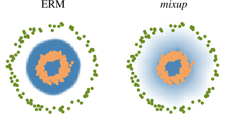
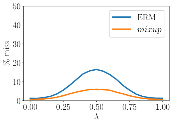
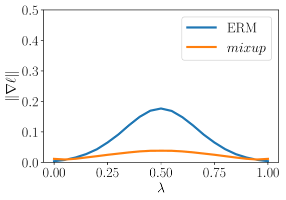
The mixup vicinal distribution can be understood as a form of data augmentation that encourages the model $f$ to behave linearly in-between training examples. We argue that this linear behaviour reduces the amount of undesirable oscillations when predicting outside the training examples. Also, linearity is a good inductive bias from the perspective of Occam’s razor, since it is one of the simplest possible behaviors. Figure 1(b) shows that mixup leads to decision boundaries that transition linearly from class to class, providing a smoother estimate of uncertainty. Figure 2 illustrate the average behaviors of two neural network models trained on the CIFAR-10 dataset using ERM and mixup. Both models have the same architecture, are trained with the same procedure, and are evaluated at the same points in-between randomly sampled training data. The model trained with mixup is more stable in terms of model predictions and gradient norms in-between training samples.

(a) Prediction errors in-between training data. Evaluated at $x=\lambda x_{i}+(1-\lambda)x_{j}$, a prediction is counted as a “miss” if it does not belong to $\{y_{i},y_{j}\}$. The model trained with mixup has fewer misses.

(b) Norm of the gradients of the model w.r.t. input in-between training data, evaluated at $x=\lambda x_{i}+(1-\lambda)x_{j}$. The model trained with mixup has smaller gradient norms.

Figure 2: mixup leads to more robust model behaviors in-between the training data.

3 Experiments

3.1 ImageNet classification

We evaluate mixup on the ImageNet-2012 classification dataset (Russakovsky et al., 2015). This dataset contains 1.3 million training images and 50,000 validation images, from a total of 1,000 classes. For training, we follow standard data augmentation practices: scale and aspect ratio distortions, random crops, and horizontal flips (Goyal et al., 2017). During evaluation, only the $224\times 224$ central crop of each image is tested. We use mixup and ERM to train several state-of-the-art ImageNet-2012 classification models, and report both top-1 and top-5 error rates in Table 1.

Model	Method	Epochs	Top-1 Error	Top-5 Error
ResNet-50	ERM (Goyal et al., 2017)	$90$	$23.5$	-
	mixup $\alpha=0.2$	$90$	$\bf 23.3$	$\bf 6.6$
ResNet-101	ERM (Goyal et al., 2017)	$90$	$22.1$	-
	mixup $\alpha=0.2$	$90$	$\bf 21.5$	$\bf 5.6$
ResNeXt-101 32*4d	ERM (Xie et al., 2016)	$100$	$21.2$	-
	ERM	$90$	$21.2$	$5.6$
	mixup $\alpha=0.4$	$90$	$\bf 20.7$	$\bf 5.3$
ResNeXt-101 64*4d	ERM (Xie et al., 2016)	$100$	$20.4$	$5.3$
	mixup $\alpha=0.4$	$90$	$\bf 19.8$	$\bf 4.9$
ResNet-50	ERM	$200$	$23.6$	$7.0$
	mixup $\alpha=0.2$	$200$	$\bf 22.1$	$\bf 6.1$
ResNet-101	ERM	$200$	$22.0$	$6.1$
	mixup $\alpha=0.2$	$200$	$\bf 20.8$	$\bf 5.4$
ResNeXt-101 32*4d	ERM	$200$	$21.3$	$5.9$
	mixup $\alpha=0.4$	$200$	$\bf 20.1$	$\bf 5.0$

Table 1: Validation errors for ERM and mixup on the development set of ImageNet-2012.

For all the experiments in this section, we use data-parallel distributed training in Caffe2 with a minibatch size of 1,024. We use the learning rate schedule described in (Goyal et al., 2017). Specifically, the learning rate is increased linearly from 0.1 to 0.4 during the first 5 epochs, and it is then divided by 10 after 30, 60 and 80 epochs when training for 90 epochs; or after 60, 120 and 180 epochs when training for 200 epochs.

For mixup, we find that $\alpha\in[0.1,0.4]$ leads to improved performance over ERM, whereas for large $\alpha$, mixup leads to underfitting. We also find that models with higher capacities and/or longer training runs are the ones to benefit the most from mixup. For example, when trained for 90 epochs, the mixup variants of ResNet-101 and ResNeXt-101 obtain a greater improvement (0.5% to 0.6%) over their ERM analogues than the gain of smaller models such as ResNet-50 (0.2%). When trained for 200 epochs, the top-1 error of the mixup variant of ResNet-50 is further reduced by 1.2% compared to the 90 epoch run, whereas its ERM analogue stays the same.

3.2 CIFAR-10 and CIFAR-100

We conduct additional image classification experiments on the CIFAR-10 and CIFAR-100 datasets to further evaluate the generalization performance of mixup. In particular, we compare ERM and mixup training for: PreAct ResNet-18 (He et al., 2016) as implemented in (Liu, 2017), WideResNet-28-10 (Zagoruyko & Komodakis, 2016a) as implemented in (Zagoruyko & Komodakis, 2016b), and DenseNet (Huang et al., 2017) as implemented in (Veit, 2017). For DenseNet, we change the growth rate to 40 to follow the DenseNet-BC-190 specification from (Huang et al., 2017). For mixup, we fix $\alpha=1$, which results in interpolations $\lambda$ uniformly distributed between zero and one. All models are trained on a single Nvidia Tesla P100 GPU using PyTorch for 200 epochs on the training set with 128 examples per minibatch, and evaluated on the test set. Learning rates start at 0.1 and are divided by 10 after 100 and 150 epochs for all models except WideResNet. For WideResNet, we follow (Zagoruyko & Komodakis, 2016a) and divide the learning rate by 10 after 60, 120 and 180 epochs. Weight decay is set to $10^{-4}$. We do not use dropout in these experiments.

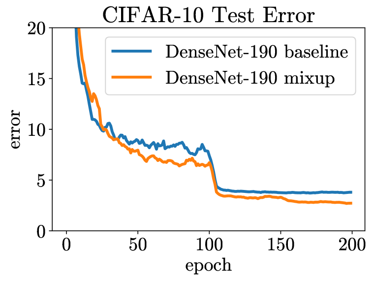
We summarize our results in Figure 3(a). In both CIFAR-10 and CIFAR-100 classification problems, the models trained using mixup significantly outperform their analogues trained with ERM. As seen in Figure 3(b), mixup and ERM converge at a similar speed to their best test errors. Note that the DenseNet models in (Huang et al., 2017) were trained for 300 epochs with further learning rate decays scheduled at the 150 and 225 epochs, which may explain the discrepancy the performance of DenseNet reported in Figure 3(a) and the original result of Huang et al. (2017).

Dataset	Model	ERM	mixup
CIFAR-10	PreAct ResNet-18	$5.6$	$\bf 4.2$
	WideResNet-28-10	$3.8$	$\bf 2.7$
	DenseNet-BC-190	$3.7$	$\bf 2.7$
CIFAR-100	PreAct ResNet-18	$25.6$	$\bf 21.1$
	WideResNet-28-10	$19.4$	$\bf 17.5$
	DenseNet-BC-190	$19.0$	$\bf 16.8$

(a) Test errors for the CIFAR experiments.

(b) Test error evolution for the best ERM and mixup models.

Figure 3: Test errors for ERM and mixup on the CIFAR experiments.

3.3 Speech data

Next, we perform speech recognition experiments using the Google commands dataset (Warden, 2017). The dataset contains 65,000 utterances, where each utterance is about one-second long and belongs to one out of 30 classes. The classes correspond to voice commands such as yes, no, down, left, as pronounced by a few thousand different speakers. To preprocess the utterances, we first extract normalized spectrograms from the original waveforms at a sampling rate of 16 kHz. Next, we zero-pad the spectrograms to equalize their sizes at $160\times 101$. For speech data, it is reasonable to apply mixup both at the waveform and spectrogram levels. Here, we apply mixup at the spectrogram level just before feeding the data to the network.

For this experiment, we compare a LeNet (Lecun et al., 2001) and a VGG-11 (Simonyan & Zisserman, 2015) architecture, each of them composed by two convolutional and two fully-connected layers. We train each model for 30 epochs with minibatches of 100 examples, using Adam as the optimizer (Kingma & Ba, 2015). Training starts with a learning rate equal to $3\times 10^{-3}$ and is divided by 10 every 10 epochs. For mixup, we use a warm-up period of five epochs where we train the network on original training examples, since we find it speeds up initial convergence. Table 4 shows that mixup outperforms ERM on this task, specially when using VGG-11, the model with larger capacity.

Model	Method	Validation set	Test set
LeNet	ERM	$\bf 9.8$	$\bf 10.3$
	mixup $(\alpha=0.1)$	$10.1$	$10.8$
	mixup $(\alpha=0.2)$	$10.2$	$11.3$
VGG-11	ERM	$5.0$	$4.6$
	mixup $(\alpha=0.1)$	$4.0$	$3.8$
	mixup $(\alpha=0.2)$	$\bf 3.9$	$\bf 3.4$

Figure 4: Classification errors of ERM and mixup on the Google commands dataset.

3.4 Memorization of corrupted labels

Following Zhang et al. (2017), we evaluate the robustness of ERM and mixup models against randomly corrupted labels. We hypothesize that increasing the strength of mixup interpolation $\alpha$ should generate virtual examples further from the training examples, making memorization more difficult to achieve. In particular, it should be easier to learn interpolations between real examples compared to memorizing interpolations involving random labels. We adapt an open-source implementation (Zhang, 2017) to generate three CIFAR-10 training sets, where 20%, 50%, or 80% of the labels are replaced by random noise, respectively. All the test labels are kept intact for evaluation. Dropout (Srivastava et al., 2014) is considered the state-of-the-art method for learning with corrupted labels (Arpit et al., 2017). Thus, we compare in these experiments mixup, dropout, mixup + dropout, and ERM. For mixup, we choose $\alpha\in\{1,2,8,32\}$; for dropout, we add one dropout layer in each PreAct block after the ReLU activation layer between two convolution layers, as suggested in (Zagoruyko & Komodakis, 2016a). We choose the dropout probability $p\in\{0.5,0.7,0.8,0.9\}$. For the combination of mixup and dropout, we choose $\alpha\in\{1,2,4,8\}$ and $p\in\{0.3,0.5,0.7\}$. These experiments use the PreAct ResNet-18 (He et al., 2016) model implemented in (Liu, 2017). All the other settings are the same as in Section 3.2.

We summarize our results in Table 2, where we note the best test error achieved during the training session, as well as the final test error after 200 epochs. To quantify the amount of memorization, we also evaluate the training errors at the last epoch on real labels and corrupted labels. As the training progresses with a smaller learning rate (e.g. less than 0.01), the ERM model starts to overfit the corrupted labels. When using a large probability (e.g. 0.7 or 0.8), dropout can effectively reduce overfitting. mixup with a large $\alpha$ (e.g. 8 or 32) outperforms dropout on both the best and last epoch test errors, and achieves lower training error on real labels while remaining resistant to noisy labels. Interestingly, mixup + dropout performs the best of all, showing that the two methods are compatible.

Label corruption	Method	Test error		Training error
		Best	Last	Real	Corrupted
20%	ERM	$12.7$	$16.6$	$0.05$	$0.28$
	ERM + dropout ($p=0.7$)	$8.8$	$10.4$	$5.26$	$83.55$
	mixup ($\alpha=8$)	$\bf 5.9$	$6.4$	$2.27$	$86.32$
	mixup + dropout ($\alpha=4,p=0.1$)	$6.2$	$\bf 6.2$	$1.92$	$85.02$
50%	ERM	$18.8$	$44.6$	$0.26$	$0.64$
	ERM + dropout ($p=0.8$)	$14.1$	$15.5$	$12.71$	$86.98$
	mixup ($\alpha=32$)	$11.3$	$12.7$	$5.84$	$85.71$
	mixup + dropout ($\alpha=8,p=0.3$)	$\bf 10.9$	$\bf 10.9$	$7.56$	$87.90$
80%	ERM	$36.5$	$73.9$	$0.62$	$0.83$
	ERM + dropout ($p=0.8$)	$30.9$	$35.1$	$29.84$	$86.37$
	mixup ($\alpha=32$)	$25.3$	$30.9$	$18.92$	$85.44$
	mixup + dropout ($\alpha=8,p=0.3$)	$\bf 24.0$	$\bf 24.8$	$19.70$	$87.67$

Table 2: Results on the corrupted label experiments for the best models.

3.5 Robustness to Adversarial examples

One undesirable consequence of models trained using ERM is their fragility to adversarial examples (Szegedy et al., 2014). Adversarial examples are obtained by adding tiny (visually imperceptible) perturbations to legitimate examples in order to deteriorate the performance of the model. The adversarial noise is generated by ascending the gradient of the loss surface with respect to the legitimate example. Improving the robustness to adversarial examples is a topic of active research.

Among the several methods aiming to solve this problem, some have proposed to penalize the norm of the Jacobian of the model to control its Lipschitz constant (Drucker & Le Cun, 1992; Cisse et al., 2017; Bartlett et al., 2017; Hein & Andriushchenko, 2017). Other approaches perform data augmentation by producing and training on adversarial examples (Goodfellow et al., 2015). Unfortunately, all of these methods add significant computational overhead to ERM. Here, we show that mixup can significantly improve the robustness of neural networks without hindering the speed of ERM by penalizing the norm of the gradient of the loss w.r.t a given input along the most plausible directions (e.g. the directions to other training points). Indeed, Figure 2 shows that mixup results in models having a smaller loss and gradient norm between examples compared to vanilla ERM.

To assess the robustness of mixup models to adversarial examples, we use three ResNet-101 models: two of them trained using ERM on ImageNet-2012, and the third trained using mixup. In the first set of experiments, we study the robustness of one ERM model and the mixup model against white box attacks. That is, for each of the two models, we use the model itself to generate adversarial examples, either using the Fast Gradient Sign Method (FGSM) or the Iterative FGSM (I-FGSM) methods (Goodfellow et al., 2015), allowing a maximum perturbation of $\epsilon=4$ for every pixel. For I-FGSM, we use 10 iterations with equal step size. In the second set of experiments, we evaluate robustness against black box attacks. That is, we use the first ERM model to produce adversarial examples using FGSM and I-FGSM. Then, we test the robustness of the second ERM model and the mixup model to these examples. The results of both settings are summarized in Table 3.

For the FGSM white box attack, the mixup model is $2.7$ times more robust than the ERM model in terms of Top-1 error. For the FGSM black box attack, the mixup model is $1.25$ times more robust than the ERM model in terms of Top-1 error. Also, while both mixup and ERM are not robust to white box I-FGSM attacks, mixup is about $40\%$ more robust than ERM in the black box I-FGSM setting. Overall, mixup produces neural networks that are significantly more robust than ERM against adversarial examples in white box and black settings without additional overhead compared to ERM.

Metric	Method	FGSM	I-FGSM
Top-1	ERM	$90.7$	$99.9$
	mixup	$\bf 75.2$	$99.6$
Top-5	ERM	$63.1$	$93.4$
	mixup	$\bf 49.1$	$95.8$

(a) White box attacks.

Metric	Method	FGSM	I-FGSM
Top-1	ERM	$57.0$	$57.3$
	mixup	$\bf 46.0$	$\bf 40.9$
Top-5	ERM	$24.8$	$18.1$
	mixup	$\bf 17.4$	$\bf 11.8$

(b) Black box attacks.

Table 3: Classification errors of ERM and mixup models when tested on adversarial examples.

3.6 Tabular data

To further explore the performance of mixup on non-image data, we performed a series of experiments on six arbitrary classification problems drawn from the UCI dataset (Lichman, 2013). The neural networks in this section are fully-connected, and have two hidden layers of 128 ReLU units. The parameters of these neural networks are learned using Adam (Kingma & Ba, 2015) with default hyper-parameters, over 10 epochs of mini-batches of size 16. Table 4 shows that mixup improves the average test error on four out of the six considered datasets, and never underperforms ERM.

Dataset	ERM	mixup
Abalone	$74.0$	$73.6$
Arcene	$57.6$	$\bf 48.0$
Arrhythmia	$56.6$	$\bf 46.3$

Dataset	ERM	mixup
Htru2	$2.0$	$2.0$
Iris	$21.3$	$\bf 17.3$
Phishing	$16.3$	$15.2$

Table 4: ERM and mixup classification errors on the UCI datasets.

3.7 Stabilization of Generative Adversarial Networks (GANs)

Generative Adversarial Networks, also known as GANs (Goodfellow et al., 2014), are a powerful family of implicit generative models. In GANs, a generator and a discriminator compete against each other to model a distribution $P$. On the one hand, the generator $g$ competes to transform noise vectors $z\sim Q$ into fake samples $g(z)$ that resemble real samples $x\sim P$. On the other hand, the discriminator competes to distinguish between real samples $x$ and fake samples $g(z)$. Mathematically, training a GAN is equivalent to solving the optimization problem

$$\max_{g}\min_{d}\operatorname*{\mathbb{E}}_{x,z}\,\ell(d(x),1)+\ell(d(g(z)),0),$$

where $\ell$ is the binary cross entropy loss. Unfortunately, solving the previous min-max equation is a notoriously difficult optimization problem (Goodfellow, 2016), since the discriminator often provides the generator with vanishing gradients. We argue that mixup should stabilize GAN training because it acts as a regularizer on the gradients of the discriminator, akin to the binary classifier in Figure 1(b). Then, the smoothness of the discriminator guarantees a stable source of gradient information to the generator. The mixup formulation of GANs is:

$$\max_{g}\min_{d}\operatorname*{\mathbb{E}}_{x,z,\lambda}\,\ell(d(\lambda x+(1-\lambda)g(z)),\lambda).$$

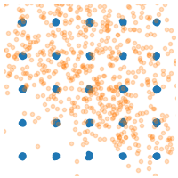
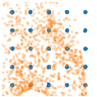
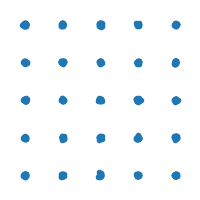
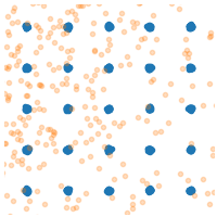
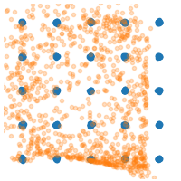
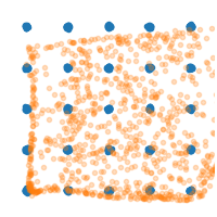
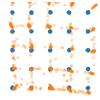
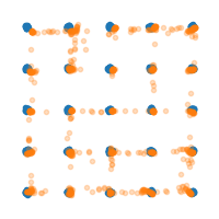
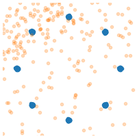
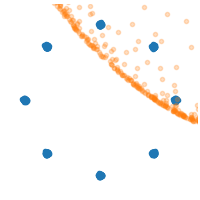
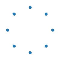
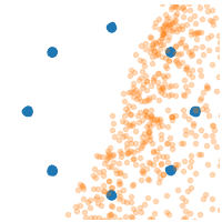
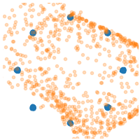
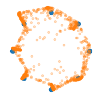
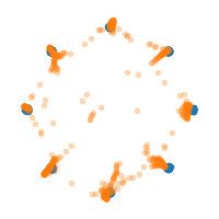
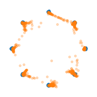
Figure 5 illustrates the stabilizing effect of mixup the training of GAN (orange samples) when modeling two toy datasets (blue samples). The neural networks in these experiments are fully-connected and have three hidden layers of 512 ReLU units. The generator network accepts two-dimensional Gaussian noise vectors. The networks are trained for 20,000 mini-batches of size 128 using the Adam optimizer with default parameters, where the discriminator is trained for five iterations before every generator iteration. The training of mixup GANs seems promisingly robust to hyper-parameter and architectural choices.

ERM GAN	mixup GAN ($\alpha=0.2$)

Figure 5: Effect of mixup on stabilizing GAN training at iterations 10, 100, 1000, 10000, and 20000.

3.8 Ablation Studies

mixup is a data augmentation method that consists of only two parts: random convex combination of raw inputs, and correspondingly, convex combination of one-hot label encodings. However, there are several design choices to make. For example, on how to augment the inputs, we could have chosen to interpolate the latent representations (i.e. feature maps) of a neural network, and we could have chosen to interpolate only between the nearest neighbors, or only between inputs of the same class. When the inputs to interpolate come from two different classes, we could have chosen to assign a single label to the synthetic input, for example using the label of the input that weights more in the convex combination. To compare mixup with these alternative possibilities, we run a set of ablation study experiments using the PreAct ResNet-18 architecture on the CIFAR-10 dataset.

Specifically, for each of the data augmentation methods, we test two weight decay settings ($10^{-4}$ which works well for mixup, and $5\times 10^{-4}$ which works well for ERM). All the other settings and hyperparameters are the same as reported in Section 3.2.

Method	Specification	Modified		Weight decay
		Input	Target	$10^{-4}$	$5\times 10^{-4}$
ERM		✗	✗	$5.53$	$5.18$
mixup	AC + RP	✓	✓	$\bf 4.24$	$4.68$
	AC + KNN	✓	✓	$4.98$	$5.26$
mix labels and latent	Layer 1	✓	✓	$4.44$	$\bf 4.51$
representations	Layer 2	✓	✓	$4.56$	$4.61$
(AC + RP)	Layer 3	✓	✓	$5.39$	$5.55$
	Layer 4	✓	✓	$5.95$	$5.43$
	Layer 5	✓	✓	$5.39$	$5.15$
mix inputs only	SC + KNN (Chawla et al., 2002)	✓	✗	$5.45$	$5.52$
	AC + KNN	✓	✗	$5.43$	$5.48$
	SC + RP	✓	✗	$5.23$	$5.55$
	AC + RP	✓	✗	$5.17$	$5.72$
label smoothing	$\epsilon=0.05$	✗	✓	$5.25$	$5.02$
(Szegedy et al., 2016)	$\epsilon=0.1$	✗	✓	$5.33$	$5.17$
	$\epsilon=0.2$	✗	✓	$5.34$	$5.06$
mix inputs +	$\epsilon=0.05$	✓	✓	$5.02$	$5.40$
label smoothing	$\epsilon=0.1$	✓	✓	$5.08$	$5.09$
(AC + RP)	$\epsilon=0.2$	✓	✓	$4.98$	$5.06$
	$\epsilon=0.4$	✓	✓	$5.25$	$5.39$
add Gaussian noise	$\sigma=0.05$	✓	✗	$5.53$	$5.04$
to inputs	$\sigma=0.1$	✓	✗	$6.41$	$5.86$
	$\sigma=0.2$	✓	✗	$7.16$	$7.24$

Table 5: Results of the ablation studies on the CIFAR-10 dataset. Reported are the median test errors of the last 10 epochs. A tick (✓) means the component is different from standard ERM training, whereas a cross (✗) means it follows the standard training practice. AC: mix between all classes. SC: mix within the same class. RP: mix between random pairs. KNN: mix between k-nearest neighbors (k=200). Please refer to the text for details about the experiments and interpretations.

To compare interpolating raw inputs with interpolating latent representations, we test on random convex combination of the learned representations before each residual block (denoted Layer 1-4) or before the uppermost “average pooling + fully connected” layer (denoted Layer 5). To compare mixing random pairs of inputs (RP) with mixing nearest neighbors (KNN), we first compute the 200 nearest neighbors for each training sample, either from the same class (SC) or from all the classes (AC). Then during training, for each sample in a minibatch, we replace the sample with a synthetic sample by convex combination with a random draw from its nearest neighbors. To compare mixing all the classes (AC) with mixing within the same class (SC), we convex combine a minibatch with a random permutation of its sample index, where the permutation is done in a per-batch basis (AC) or a per-class basis (SC). To compare mixing inputs and labels with mixing inputs only, we either use a convex combination of the two one-hot encodings as the target, or select the one-hot encoding of the closer training sample as the target. For label smoothing, we follow Szegedy et al. (2016) and use $\frac{\epsilon}{10}$ as the target for incorrect classes, and $1-\frac{9\epsilon}{10}$ as the target for the correct class.　Adding Gaussian noise to inputs is used as another baseline. We report the median test errors of the last 10 epochs. Results are shown in Table 5.

From the ablation study experiments, we have the following observations. First, mixup is the best data augmentation method we test, and is significantly better than the second best method (mix input + label smoothing). Second, the effect of regularization can be seen by comparing the test error with a small weight decay ($10^{-4}$) with a large one ($5\times 10^{-4}$). For example, for ERM a large weight decay works better, whereas for mixup a small weight decay is preferred, confirming its regularization effects. We also see an increasing advantage of large weight decay when interpolating in higher layers of latent representations, indicating decreasing strength of regularization. Among all the input interpolation methods, mixing random pairs from all classes (AC + RP) has the strongest regularization effect. Label smoothing and adding Gaussian noise have a relatively small regularization effect. Finally, we note that the SMOTE algorithm (Chawla et al., 2002) does not lead to a noticeable gain in performance.

4 Related Work

Data augmentation lies at the heart of all successful applications of deep learning, ranging from image classification (Krizhevsky et al., 2012) to speech recognition (Graves et al., 2013; Amodei et al., 2016). In all cases, substantial domain knowledge is leveraged to design suitable data transformations leading to improved generalization. In image classification, for example, one routinely uses rotation, translation, cropping, resizing, flipping (Lecun et al., 2001; Simonyan & Zisserman, 2015), and random erasing (Zhong et al., 2017) to enforce visually plausible invariances in the model through the training data. Similarly, in speech recognition, noise injection is a prevalent practice to improve the robustness and accuracy of the trained models (Amodei et al., 2016).

More related to mixup, Chawla et al. (2002) propose to augment the rare class in an imbalanced dataset by interpolating the nearest neighbors; DeVries & Taylor (2017) show that interpolation and extrapolation the nearest neighbors of the same class in feature space can improve generalization. However, their proposals only operate among the nearest neighbors within a certain class at the input / feature level, and hence does not account for changes in the corresponding labels. Recent approaches have also proposed to regularize the output distribution of a neural network by label smoothing (Szegedy et al., 2016), or penalizing high-confidence softmax distributions (Pereyra et al., 2017). These methods bear similarities with mixup in the sense that supervision depends on multiple smooth labels, rather than on single hard labels as in traditional ERM. However, the label smoothing in these works is applied or regularized independently from the associated feature values.

mixup enjoys several desirable aspects of previous data augmentation and regularization schemes without suffering from their drawbacks. Like the method of DeVries & Taylor (2017), it does not require significant domain knowledge. Like label smoothing, the supervision of every example is not overly dominated by the ground-truth label. Unlike both of these approaches, the mixup transformation establishes a linear relationship between data augmentation and the supervision signal. We believe that this leads to a strong regularizer that improves generalization as demonstrated by our experiments. The linearity constraint, through its effect on the derivatives of the function approximated, also relates mixup to other methods such as Sobolev training of neural networks (Czarnecki et al., 2017) or WGAN-GP (Gulrajani et al., 2017).

5 Discussion

We have proposed mixup, a data-agnostic and straightforward data augmentation principle. We have shown that mixup is a form of vicinal risk minimization, which trains on virtual examples constructed as the linear interpolation of two random examples from the training set and their labels. Incorporating mixup into existing training pipelines reduces to a few lines of code, and introduces little or no computational overhead. Throughout an extensive evaluation, we have shown that mixup improves the generalization error of state-of-the-art models on ImageNet, CIFAR, speech, and tabular datasets. Furthermore, mixup helps to combat memorization of corrupt labels, sensitivity to adversarial examples, and instability in adversarial training.

In our experiments, the following trend is consistent: with increasingly large $\alpha$, the training error on real data increases, while the generalization gap decreases. This sustains our hypothesis that mixup implicitly controls model complexity. However, we do not yet have a good theory for understanding the ‘sweet spot’ of this bias-variance trade-off. For example, in CIFAR-10 classification we can get very low training error on real data even when $\alpha\to\infty$ (i.e., training only on averages of pairs of real examples), whereas in ImageNet classification, the training error on real data increases significantly with $\alpha\to\infty$. Based on our ImageNet and Google commands experiments with different model architectures, we conjecture that increasing the model capacity would make training error less sensitive to large $\alpha$, hence giving mixup a more significant advantage.

mixup also opens up several possibilities for further exploration. First, is it possible to make similar ideas work on other types of supervised learning problems, such as regression and structured prediction? While generalizing mixup to regression problems is straightforward, its application to structured prediction problems such as image segmentation remains less obvious. Second, can similar methods prove helpful beyond supervised learning? The interpolation principle seems like a reasonable inductive bias which might also help in unsupervised, semi-supervised, and reinforcement learning. Can we extend mixup to feature-label extrapolation to guarantee a robust model behavior far away from the training data? Although our discussion of these directions is still speculative, we are excited about the possibilities mixup opens up, and hope that our observations will prove useful for future development.

References

- Amodei et al. (2016) D. Amodei, S. Ananthanarayanan, R. Anubhai, J. Bai, E. Battenberg, C. Case, J. Casper, B. Catanzaro, Q. Cheng, G. Chen, et al. Deep speech 2: End-to-end speech recognition in English and Mandarin. In ICML, 2016.
- Arpit et al. (2017) D. Arpit, S. Jastrzebski, N. Ballas, D. Krueger, E. Bengio, M. S. Kanwal, T. Maharaj, A. Fischer, A. Courville, Y. Bengio, et al. A closer look at memorization in deep networks. ICML, 2017.
- Bartlett et al. (2017) P. Bartlett, D. J. Foster, and M. Telgarsky. Spectrally-normalized margin bounds for neural networks. NIPS, 2017.
- Chapelle et al. (2000) O. Chapelle, J. Weston, L. Bottou, and V. Vapnik. Vicinal risk minimization. NIPS, 2000.
- Chawla et al. (2002) N. V. Chawla, K. W. Bowyer, L. O. Hall, and W. P. Kegelmeyer. SMOTE: synthetic minority over-sampling technique. Journal of artificial intelligence research, 16:321–357, 2002.
- Chelba et al. (2013) C. Chelba, T. Mikolov, M. Schuster, Q. Ge, T. Brants, P. Koehn, and T. Robinson. One billion word benchmark for measuring progress in statistical language modeling. arXiv, 2013.
- Cisse et al. (2017) M. Cisse, P. Bojanowski, E. Grave, Y. Dauphin, and N. Usunier. Parseval networks: Improving robustness to adversarial examples. ICML, 2017.
- Czarnecki et al. (2017) W. M. Czarnecki, S. Osindero, M. Jaderberg, G. Świrszcz, and R. Pascanu. Sobolev training for neural networks. NIPS, 2017.
- DeVries & Taylor (2017) T. DeVries and G. W. Taylor. Dataset augmentation in feature space. ICLR Workshops, 2017.
- Drucker & Le Cun (1992) H. Drucker and Y. Le Cun. Improving generalization performance using double backpropagation. IEEE Transactions on Neural Networks, 3(6):991–997, 1992.
- Goodfellow (2016) I. Goodfellow. Tutorial: Generative adversarial networks. NIPS, 2016.
- Goodfellow et al. (2014) I. Goodfellow, J. Pouget-Abadie, M. Mirza, B. Xu, D. Warde-Farley, S. Ozair, A. Courville, and Y. Bengio. Generative adversarial nets. NIPS, 2014.
- Goodfellow et al. (2015) I. J. Goodfellow, J. Shlens, and C. Szegedy. Explaining and harnessing adversarial examples. ICLR, 2015.
- Goyal et al. (2017) P. Goyal, P. Dollár, R. Girshick, P. Noordhuis, L. Wesolowski, A. Kyrola, A. Tulloch, Y. Jia, and K. He. Accurate, large minibatch SGD: Training ImageNet in 1 hour. arXiv, 2017.
- Graves et al. (2013) A. Graves, A.-r. Mohamed, and G. Hinton. Speech recognition with deep recurrent neural networks. In ICASSP. IEEE, 2013.
- Gulrajani et al. (2017) I. Gulrajani, F. Ahmed, M. Arjovsky, V. Dumoulin, and A. Courville. Improved training of Wasserstein GANs. NIPS, 2017.
- Harvey et al. (2017) N. Harvey, C. Liaw, and A. Mehrabian. Nearly-tight VC-dimension bounds for piecewise linear neural networks. JMLR, 2017.
- He et al. (2016) K. He, X. Zhang, S. Ren, and J. Sun. Identity mappings in deep residual networks. ECCV, 2016.
- Hein & Andriushchenko (2017) M. Hein and M. Andriushchenko. Formal guarantees on the robustness of a classifier against adversarial manipulation. NIPS, 2017.
- Hinton et al. (2012) G. Hinton, L. Deng, D. Yu, G. E. Dahl, A.-r. Mohamed, N. Jaitly, A. Senior, V. Vanhoucke, P. Nguyen, T. N. Sainath, et al. Deep neural networks for acoustic modeling in speech recognition: The shared views of four research groups. IEEE Signal Processing Magazine, 2012.
- Huang et al. (2017) G. Huang, Z. Liu, L. van der Maaten, and K. Q. Weinberger. Densely connected convolutional networks. CVPR, 2017.
- Kingma & Ba (2015) D. Kingma and J. Ba. Adam: A method for stochastic optimization. ICLR, 2015.
- Krizhevsky et al. (2012) A. Krizhevsky, I. Sutskever, and G. E. Hinton. ImageNet classification with deep convolutional neural networks. NIPS, 2012.
- Lecun et al. (2001) Y. Lecun, L. Bottou, Y. Bengio, and P. Haffner. Gradient-based learning applied to document recognition. Proceedings of IEEE, 2001.
- Lichman (2013) M. Lichman. UCI machine learning repository, 2013.
- Liu (2017) K. Liu, 2017. URL https://github.com/kuangliu/pytorch-cifar.
- Pereyra et al. (2017) G. Pereyra, G. Tucker, J. Chorowski, Ł. Kaiser, and G. Hinton. Regularizing neural networks by penalizing confident output distributions. ICLR Workshops, 2017.
- Russakovsky et al. (2015) O. Russakovsky, J. Deng, H. Su, J. Krause, S. Satheesh, S. Ma, Z. Huang, A. Karpathy, A. Khosla, M. Bernstein, A. C. Berg, and L. Fei-Fei. ImageNet large scale visual recognition challenge. IJCV, 2015.
- Silver et al. (2016) D. Silver, A. Huang, C. J. Maddison, A. Guez, L. Sifre, G. Van Den Driessche, J. Schrittwieser, I. Antonoglou, V. Panneershelvam, M. Lanctot, et al. Mastering the game of Go with deep neural networks and tree search. Nature, 2016.
- Simard et al. (1998) P. Simard, Y. LeCun, J. Denker, and B. Victorri. Transformation invariance in pattern recognition—tangent distance and tangent propagation. Neural networks: tricks of the trade, 1998.
- Simonyan & Zisserman (2015) K. Simonyan and A. Zisserman. Very deep convolutional networks for large-scale image recognition. ICLR, 2015.
- Springenberg et al. (2015) J. T. Springenberg, A. Dosovitskiy, T. Brox, and M. Riedmiller. Striving for simplicity: The all convolutional net. ICLR Workshops, 2015.
- Srivastava et al. (2014) N. Srivastava, G. E. Hinton, A. Krizhevsky, I. Sutskever, and R. Salakhutdinov. Dropout: a simple way to prevent neural networks from overfitting. Journal of Machine Learning Research, 15(1):1929–1958, 2014.
- Szegedy et al. (2014) C. Szegedy, W. Zaremba, I. Sutskever, J. Bruna, D. Erhan, I. J. Goodfellow, and R. Fergus. Intriguing properties of neural networks. ICLR, 2014.
- Szegedy et al. (2016) C. Szegedy, V. Vanhoucke, S. Ioffe, J. Shlens, and Z. Wojna. Rethinking the Inception architecture for computer vision. Proceedings of the IEEE Conference on Computer Vision and Pattern Recognition, 2016.
- Vapnik (1998) V. N. Vapnik. Statistical learning theory. J. Wiley, 1998.
- Vapnik & Chervonenkis (1971) V. Vapnik and A. Y. Chervonenkis. On the uniform convergence of relative frequencies of events to their probabilities. Theory of Probability and its Applications, 1971.
- Veit (2017) A. Veit, 2017. URL https://github.com/andreasveit.
- Warden (2017) P. Warden, 2017. URL https://research.googleblog.com/2017/08/launching-speech-commands-dataset.html.
- Xie et al. (2016) S. Xie, R. Girshick, P. Dollár, Z. Tu, and K. He. Aggregated residual transformations for deep neural networks. CVPR, 2016.
- Zagoruyko & Komodakis (2016a) S. Zagoruyko and N. Komodakis. Wide residual networks. BMVC, 2016a.
- Zagoruyko & Komodakis (2016b) S. Zagoruyko and N. Komodakis, 2016b. URL https://github.com/szagoruyko/wide-residual-networks.
- Zhang et al. (2017) C. Zhang, S. Bengio, M. Hardt, B. Recht, and O. Vinyals. Understanding deep learning requires rethinking generalization. ICLR, 2017.
- Zhang (2017) C. Zhang, 2017. URL https://github.com/pluskid/fitting-random-labels.
- Zhong et al. (2017) Z. Zhong, L. Zheng, G. Kang, S. Li, and Y. Yang. Random erasing data augmentation. arXiv, 2017.