Estimating the Operating Characteristics of Ensemble Methods

Abstract

Suppose we would like to compare the performance of two binary classification algorithms. If we have their receiver operating characteristic (ROC) curves, then one might conclude that the algorithm corresponding to the higher ROC curve is better. This conclusion may not be correct due to variability in the ROC curves. Two sources of variability are randomness in the procedure used to train each classifier and randomness in the sample of feature vectors that form the test data set.

In this paper we present a technique for using the bootstrap to estimate the operating characteristics and their variability for certain types of ensemble methods. Bootstrapping a model can require a huge amount of work if the training data set is large. Fortunately in many cases the technique lets us determine the effect of infinite resampling without actually refitting a single model. We apply the technique to the study of meta-parameter selection for random forests. We demonstrate that alternatives to bootstrap aggregation and to considering $\sqrt{d}$ features to split each node, where $d$ is the number of features, can produce improvements in predictive accuracy.

1 Introduction

Suppose we would like to compare the performance of two binary classification algorithms. The receiver operating characteristic (ROC) curve for each algorithm is shown in Figure 1. A ROC curve is simply a plot of the true positive rate (TPR) against the false positive rate (FPR) as the discrimination threshold is varied.

Figure 1: ROC curves for two binary classifiers. Which algorithm is better?

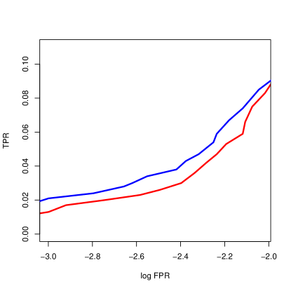
The obvious conclusion is that since the blue ROC curve is higher, the corresponding algorithm must be better. In this case the conclusion is not correct. Both ROC curves were produced using the same algorithm, the same training data set, and the same test data set. The difference in the ROC curves is entirely due to randomness in various choices made by the algorithm during training. See Section 3.2 for a complete description of how this example was generated.

An ensemble method combines multiple weak learners to obtain better predictive performance than could be obtained from any of the individual learners alone [9]. For example, a random forest uses an ensemble of decision trees. Each tree casts a vote and the forest combines the votes to get a final prediction.

In this paper we describe a computationally efficient technique for estimating the variability in ROC curves for ensemble methods that base their decision on a vote among the weak classifiers. The main idea is to bootstrap the weak classifiers and to Poisson bootstrap [3] the feature vectors in the test set. Note that the technique has some ideas in common with previous unpublished work done by Gamst and Goldschmidt.

Bootstrapping a model can require a huge amount of work if we need to repeatedly fit the model to large data sets. Fortunately in many cases the technique described here lets us determine the effect of doing infinite resampling without actually refitting a single model.

The rest of the paper is organized as follows. In Section 2 we describe the technique for generating a ROC curve and for estimating its variability. In Section 3 we describe various examples of applying the new technique. Finally in Section 4 we give some conclusions as well as directions for future work.

2 Resampling the Weak Classifiers and the Test Set

Let $X$ be the feature space and let $\mathcal{F}$ be a (possibly infinite) set of binary classifiers on $X$. Let $\mu_{\mathcal{F}}$ be a measure on $\mathcal{F}$. We construct an ensemble method $\gamma$ by sampling $m$ weak classifiers $f_{1},\ldots,f_{m}$ independently from $\mathcal{F}$ according to $\mu_{\mathcal{F}}$. Then for each $t\in[0,m]$ the class label assigned to $x$ with threshold $t$ is:

$$\hat{y}(x|\gamma,t) =1,\mbox{if}\sum_{i=1}^{m}f_{i}(x)\geq t,\mbox{and}$$

$$=0,\mbox{otherwise}.$$

In other words, $\gamma$ predicts that $x$ is positive with threshold $t$ if and only if at least $t$ of its weak classifiers predict that $x$ is positive.

Let $X\times Y$ be a (possibly infinite) space of labeled feature vectors. Let $\mu_{X\times Y}$ be a measure on $X\times Y$. We evaluate the ensemble method $F$ as follows. First we sample $N$ labeled feature vectors $(x_{1},y_{1}),\ldots,(x_{N},y_{N})$ independently from $X\times Y$ according to $\mu_{X\times Y}$. Then for each $t\in[0,m]$ we compute:

$$\mbox{FPR}(\gamma,t) =\frac{|\{(x_{j},y_{j}):\hat{y}(x_{j}|\gamma,t)=1\mbox{\ and\ }y_{j}=0\}|}{|\{(x_{j},y_{j}):y_{j}=0\}|}.$$

$$\mbox{TPR}(\gamma,t) =\frac{|\{(x_{j},y_{j}):\hat{y}(x_{j}|\gamma,t)=1\mbox{\ and\ }y_{j}=1\}|}{|\{(x_{j},y_{j}):y_{j}=1\}|}.$$

For each $t$ we plot FPR($\gamma,t$) against TPR($\gamma,t$) to obtain a ROC curve.

Note that a standard random forest fits this description. Each time a decision tree is produced, some randomness is introduced by varying the bootstrapped sample of training feature vectors and the features considered for splitting each node. $\mathcal{F}$ is the space of all possible decision trees that could have been produced from the training data, and $\mu_{\mathcal{F}}$ gives the probability of producing each decision tree. We assume the $N$ test feature vectors were drawn from a space of labeled feature vectors according to some measure $\mu_{X\times Y}$.

The estimate of the ROC curve depends on which $f_{i}$ and which $(x_{j},y_{j})$ we happened to sample. Ideally we would like to know the average ROC curve across all possible samples $\{f_{i}\}$ and $\{(x_{j},y_{j})\}$. Since compute and data limits prevent us from obtaining arbitrarily many $f_{i}$ and $(x_{j},y_{j})$ we turn to resampling techniques instead.

2.1 Resampling the Weak Classifiers

Let $p_{x_{j}}=\Pr[f(x_{j})=1]$ where $f$ is chosen randomly from $\mathcal{F}$ according to $\mu_{\mathcal{F}}$. Then

$$\Pr[\hat{y}(x_{j}|\gamma,t)=1]=\sum_{k=t}^{m}\binom{m}{k}p_{x_{j}}^{k}(1-p_{x_{j}})^{m-k}.$$

For each $x_{j}$ in the test set we can use the empirical estimate:

$$p_{x_{j}}\simeq\frac{1}{m}|\{f_{i}:f_{i}(x_{j})=1\}|.$$

The estimates of FPR and TPR then become:

$$\mbox{FPR}(\gamma,t) =\frac{\sum_{j=1}^{N}\Pr[\hat{y}(x_{j}|\gamma,t)=1]\chi(y_{j}=0)}{|\{(x_{j},y_{j}):y_{j}=0\}|}.$$

$$\mbox{TPR}(\gamma,t) =\frac{\sum_{j=1}^{N}\Pr[\hat{y}(x_{j}|\gamma,t)=1]\chi(y_{j}=1)}{|\{(x_{j},y_{j}):y_{j}=1\}|}.$$

Here $\chi()$ is the indicator function that has value one when the statement is true and zero otherwise.

The idea is to account for the variability from the choice of $\{f_{i}\}$. If a test feature vector $x_{j}$ received $k$ positive votes, then it might have received fewer or more votes from a different sample of $\{f_{i}\}$. Thus $x_{j}$ has some probability of satisfying a higher threshold than $k$ or of not satisfying a lower threshold. We can also estimate the variance in FPR($\gamma$) and TPR($\gamma$) since they are produced by summing i.i.d. random variables. The formula for the variance will be given in the next section since it will also account for the variability from the choice of the test set.

2.2 Resampling the Test Set

Given one test set of $N$ feature vectors we would like to evaluate an ensemble method across many different test sets. In the absence of more data we can create a new test by sampling with replacement from the original one. To simplify calculations we will perform a Poisson bootstrap on the test set[3]. For each $(x_{j},y_{j})$ in the original test set we will put $c_{j}$ copies in the new test set where $c_{j}$ is a rate-1 Poisson random variable, i.e., $\Pr[c_{j}=k]=e^{-1}/k!$. Note that the new test set has approximately $N$ feature vectors. The quality of the approximation improves as $N$ becomes large. Now the estimates of FPR and TPR are:

$$\mbox{FPR}(\gamma,t) =\frac{\sum_{j=1}^{N}c_{j}\Pr[\hat{y}(x_{j}|\gamma,t)=1]\chi(y_{j}=0)}{|\{(x_{j},y_{j}):y_{j}=0\}|}.$$

$$\mbox{TPR}(\gamma,t) =\frac{\sum_{j=1}^{N}c_{j}\Pr[\hat{y}(x_{j}|\gamma,t)=1]\chi(y_{j}=1)}{|\{(x_{j},y_{j}):y_{j}=1\}|}.$$

Including $c_{j}$ in the above expressions doesn’t change the mean, but it does affect the variance. Let $b_{j}$ be a random variable that is 1 with probability $\Pr[\hat{y}(x_{j}|\gamma,t)=1]$ and 0 otherwise. Then

$$\mbox{Var}(c_{j}b_{j})=[E(c_{j})]^{2}\mbox{Var}(b_{j})+[E(b_{j})]^{2}\mbox{Var}(c_{j})+\mbox{Var}(b_{j})\mbox{Var}(c_{j}).$$

Let $q_{j}(t)=\Pr[\hat{y}(x_{j}|\gamma,t))=1]$. Since $E(b_{j})=q_{j}$, $\mbox{Var}(b_{j})=q_{j}(1-q_{j})$, $E(c_{j})=1$, and $\mbox{Var}(c_{j})=1$ we get:

$$\mbox{Var}(c_{j}b_{j}) =q_{j}(1-q_{j})+q_{j}^{2}+q_{j}(1-q_{j})$$

$$=q_{j}+q_{j}(1-q_{j}).$$

This represents the (unnormalized) contribution of the test feature vector $x_{j}$ sampled with multiplicity $c_{j}$ to the variance of the FPR or TPR. Note that normalizing by ${|\{(x_{j},y_{j}):y_{j}=0\}|}$ or ${|\{(x_{j},y_{j}):y_{j}=1\}|}$ is no longer correct since the Poisson resampling changes the number of test-set feature vectors in each class. However, the error introduced by the normalization should be small if $N$ is sufficiently large. To estimate Var(FPR) and Var(TPR) we assume the $b_{j}$ are independent so we can sum the variances over $j$.

2.3 Comparison of Techniques

In unpublished work, Gamst and Goldschmidt resampled the test vectors and computed the threshold $t$ corresponding to a particular FPR. They then averaged the thresholds produced from many samples. This arrangement of the work forced them to either generate each sample or to do complicated calculations with multinomial coefficients.

The technique described in this paper resampled both the test vectors and the weak classifiers. It computed the FPR and TPR corresponding to a particular threshold $t$. The advantage of arranging the work in this way was that the effect of taking infinitely many samples from the training vectors and the weak classifiers could be computed without actually generating any samples. Furthermore, most of the computation did not depend on the number $m$ of weak classifiers in the ensemble. Therefore the effect of varying the size of the ensemble could be determined for a relatively small amount of additional work.

Chamandy et. al. [3] described using the Poisson bootstrap to determine the variability in a statistic computed on an extremely large data set. They did not focus on ensemble methods and in particular they did not discuss resampling the weak classifiers in an ensemble.

3 Examples

In this section we give some examples of estimating the operating characteristics of ensemble methods.

3.1 Data

To demonstrate the technique, we wanted an interesting binary classification problem related to real-world data with a relatively large sample. We also wanted the problem to be difficult but not impossible. With that in mind, we did the following. First, we obtained the original ImageNet [5] data set of about 1.2 million images each labeled with one of 1000 classes. We took the VGG16 [7] model provided by Keras [4] and removed the top two layers. Feeding an image into the resulting model produces a feature vector of length 4096 which should provide information about the image label. Indeed, retraining the top two layers of VGG16 (a dense ReLU layer of size 4096 followed by a dense softmax layer of size 1000) quickly regains much of the accuracy of the original VGG16 model. To produce a binary classification problem, we arbitrarily made labels 0–499 correspond to class 0 and labels 500-999 correspond to class 1. Thus, our data consists of 1.2 million 4096-long feature vectors, each with a 0-1 label.

3.2 Variability Estimates

Figure 2: ROC curves for two random forest classifiers for the image data set. Each random forest was trained on 10K images and tested on 10K images. The shaded regions are approximate 95% confidence bands with and without Poisson bootstrapping the test data set. The inset shows the full ROC curve. Throughout this paper the x-axis of the ROC curves is on a log-scale and the logs are taken base-10.

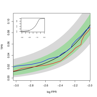
In Figure 1 both ROC curves are for a random forest with 256 trees where each tree has a maximum depth of 20. Each forest was trained on 10K images and then tested on 10K images. The difference between the red and blue ROC curves is due to each forest making different random decisions when building its decision trees. Note that for this example we intentionally used a small subset of the image data to show the variability in the ROC curves. In later examples we will usually train the random forests on 1M images and test them on 200K images. In each example each tree has a maximum depth of 20 unless otherwise indicated.

Figure 2 shows approximate 95% confidence bands for a random forest with 256 trees. The gray confidence band accounts for the variability from the choice of test data set, and the green confidence band does not. Both ROC curves from Figure 1 lie within both confidence bands, so the difference between the red and blue ROC curves is unsurprising. For the remaining examples in this paper we will not account for the variability from the choice of test data set since all of the variations of random forest used the same training data set and test data set.

The confidence bands in this example and in all subsequent examples were constructed by the following procedure. First, we built an ensemble of 4096 trees. Next we applied the technique described earlier in this paper to compute the mean and variance for each point on the ROC curve. Finally, we applied the method described in section 4.3 of [8] to produce the confidence bands, although other approaches, including those described in Sun and Loader [6] could be used.

3.3 Reduced Training Data

Figure 3: Confidence bands for random forests trained on 1M images and 200K images. Also shown are two standard deviation confidence intervals (black) for log FPR and TPR at several points along the curve. The inset shows the full ROC curves.

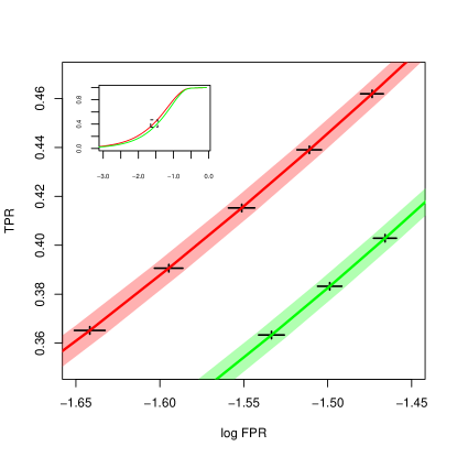
It is well known that using more training data to build a classifier usually improves its performance. This is illustrated by Figure 3 which compares the operating characteristic estimates for a random forest trained on 1M images and a random forest trained on 200K images. Reducing the amount of training data causes the random forest to perform significantly worse.

3.4 Fewer or More Trees

Figure 4: Confidence bands for random forests with 256 trees and 128 trees. Also shown are two standard deviation confidence intervals (black) for log FPR and TPR at several points along the curve. The inset shows the full ROC curves.

Figure 5: Confidence bands for random forests with 256 trees and 512 trees. Also shown are two standard deviation confidence intervals (black) for log FPR and TPR at several points along the curve. The inset shows the full ROC curves.

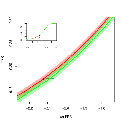
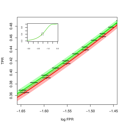
If a random forest does not have enough trees then we expect its performance to be worse. The theory of random forests asserts that adding more trees cannot (asymptotically) hurt performance. Figure 4 compares the confidence bands for 128-tree and 256-tree forests. Figure 5 compares the confidence bands for 256-tree and 512-tree forests. In both cases when the number of trees is doubled the performance of the forest improves. The gain is smaller when going from 256 trees to 512 trees suggesting that the returns from adding more trees are starting to diminish.

3.5 Bounded Tree Depth

Figure 6: Confidence bands for random forests whose trees have maximum depth 20 and maximum depth 10. Also shown are two standard deviation confidence intervals (black) for log FPR and TPR at several points along the curve. The inset shows the full ROC curves.

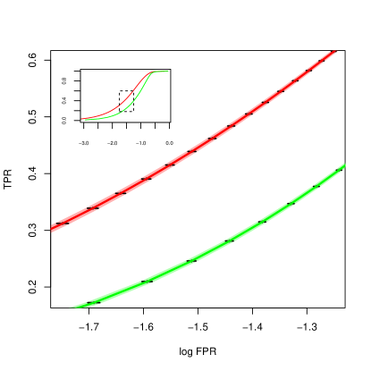
The sklearn implementation of a random forest gives the user the option to bound the depths of the trees. This reduces the size of each tree, potentially reducing the training time, testing time, and storage requirements for the forest. It may also reduce overfitting to the training data.

Figure 6 compares the operating characteristic estimates for random forests with maximum tree depths of 10 and 20. For this data set reducing the maximum tree depth hurts the performance of the forest.

This is likely to be a general phenomenon. Restricting the depth of a decision tree will increase its approximation error. An $s$-split tree for example can only approximate functions of $s$ or fewer features. Averaging has no effect on approximation error, although it does reduce estimation error. The average of noisy estimates has variance less than that of any one of the estimates; how much less depends on how correlated the various estimates are (and the size of the weights used to compute the average). So, restricted depth trees should perform worse than their expanded cousins up to the point where the approximation error is “good enough”. This trade-off is more easily balanced by setting the minimum number of observations allowed in any leaf node; that is, refusing to split if the suggested split would produce fewer than $k_{n}$ observations in either daughter node (see below). This is because splits defined over nodes with few observations are likely to be spurious, whereas the fitted trees may need to be both deep and narrow, splitting off small subsets at each level. Regardless, cross-validation and other techniques can be used to select approximately optimal values for such meta-parameters.

3.6 No Bootstrapping Training Data

Figure 7: Confidence bands for random forests trained with bootstrapping and without bootstrapping of the training data set. Also shown are two standard deviation confidence intervals (black) for log FPR and TPR at several points along the curve. The inset shows the full ROC curves.

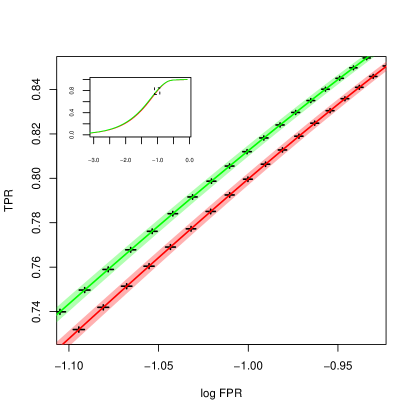
A random forest uses two ideas to reduce the correlation between trees. First, a bootstrapped sample of the training feature vectors are used to create each tree. Second, a random subset of the features is considered when splitting each node.

As a thought experiment consider a random forest with a single tree. In this case it’s not clear that we need to bootstrap the training vectors when building the tree. Furthermore, if we believe that bootstrapping is harmful for a small forest and beneficial for a large forest, then there should be some crossover point. Can we observe this crossover point, and is it smaller or larger than the forests that we actually produce?

The original purpose of the bootstrapping and averaging was to stabilize the predictions from individual trees. The structure of and classifications produced by individual trees are very sensitive to the specifics of the training data, in the sense that small changes to the training data set can produce very different trees. Bootstrap samples can be seen as small perturbations to the training data and it makes sense to trust the average tree over all perturbations than any single tree. On the other hand, this effect should vanish as the size of the training data set increases, provided the individual trees don’t grow too fast as the sample size increases. Regardless, one could consider sub-sampling or different (high-entropy) weighting schemes as alternatives to the bootstrap, using cross-validation or some other procedure to choose between the alternatives. For example, bootstrapping corresponds roughly with re-weighting the observations according to samples from a very specific distribution. This distribution can be embedded in a one-parameter exponential family and cross-validation can be used to select the optimal value for this hyper-parameter.

Figure 7 compares the operating characteristic estimates for random forests built with and without bootstrapping the training set vectors. The forest built without bootstrapping performs better.

3.7 Considering More Features to Split Each Node

Figure 8: Confidence bands for random forests trained by considering 64 features and considering 256 features when splitting each node. Also shown are two standard deviation confidence intervals (black) for log FPR and TPR at several points along the curve. The inset shows the full ROC curves.

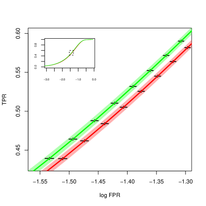
Breiman [2] recommended trying $\sqrt{d}$ features to split each node where $d$ is the number of features in the data set. Some widely-used implementations of random forests (such as sklearn) do this by default. Figure 8 compares the confidence bands for random forests that consider 64 features and 256 features to split each node. Since the image data set has 4096 features, considering 64 features is standard. However, considering 256 features clearly performs better.

4 Conclusions and Ongoing Work

We have provided a simple, computationally efficient technique for constructing ROC curves and associated confidence bands for ensemble methods. This technique could easily be extended to deal with weak learners producing non-binary output and to regression (as opposed to classification problems) and other loss functions. The technique could also be modified to deal with different aggregation techniques, by considering non-uniform weights on collections of weak learners. None of these extensions is considered here, but the bones of the technique are strong enough to support discussion and use.

We have demonstrated that there are at least two sources of variation which influence the estimated operating characteristics of a given ensemble method: the particular weak learners included in the ensemble and the particular training data set used to produce the estimates. It is important to think about both sources of error when comparing techniques or assessing the performance of a single technique.

Finally, we applied the technique to various implementations of the random forest algorithm. This produced many insights, among them: considering data resampling schemes other than the bootstrap can lead to forests with improved predictive accuracy; and artificially restricting the depth of individual trees or otherwise biasing their output will lead to worse than default performance. There are infinitely more experiments that could be carried out, but doing so would mean that this paper would never end.

References

- [1] Leo Breiman and Adele Cutler, Manual on setting up, using, and understanding Random Forest, v4.0.
- [2] L. Breiman, Random Forests. Machine Learning, 45, 5-32, 2001.
- [3] N. Chamandy, O. Muralidharan, A. Anjmi, and S. Naidu, Estimating Uncertainty for Massive Data Streams. Google Technical Report, 2012.
- [4] François Chollet, Keras, (2015), GitHub repository, https://github.com/fchollet/keras
- [5] Olga Russakovsky, Jia Deng, Hao Su, Jonathan Krause, Sanjeev Satheesh, Sean Ma, Zhiheng Huang, Andrej Karpathy, Aditya Khosla, Michael Bernstein, Alexander C. Berg and Li Fei-Fei. ImageNet Large Scale Visual Recognition Challenge. IJCV, 2015.
- [6] Jiyang Sun and Clive Loader. Simultaneous Confidence Bands for Linear Regression and Smoothing. The Annals of Statistics, 22 (2), 1328-1345, 1994.
- [7] K. Simonyan, A. Zisserman, Very Deep Convolutional Networks for Large-Scale Image Recognition. arXiv:1409.1556
- [8] W. Härdle, Applied Nonparametric Regression, Cambridge University Press, 1992.
- [9] Wikipedia:Ensemble_learning.