Modules for Experiments in Stellar Astrophysics (MESA): Convective Boundaries, Element Diffusion, and Massive Star Explosions
Abstract
We update the capabilities of the software instrument Modules for Experiments in Stellar Astrophysics (MESA) and enhance its ease of use and availability. Our new approach to locating convective boundaries is consistent with the physics of convection, and yields reliable values of the convective core mass during both hydrogen and helium burning phases. Stars with become white dwarfs and cool to the point where the electrons are degenerate and the ions are strongly coupled, a realm now available to study with MESA due to improved treatments of element diffusion, latent heat release, and blending of equations of state. Studies of the final fates of massive stars are extended in MESA by our addition of an approximate Riemann solver that captures shocks and conserves energy to high accuracy during dynamic epochs. We also introduce a 1D capability for modeling the effects of Rayleigh-Taylor instabilities that, in combination with the coupling to a public version of the STELLA radiation transfer instrument, creates new avenues for exploring Type II supernovae properties. These capabilities are exhibited with exploratory models of pair-instability supernova, pulsational pair-instability supernova, and the formation of stellar mass black holes. The applicability of MESA is now widened by the capability of importing multi-dimensional hydrodynamic models into MESA. We close by introducing software modules for handling floating point exceptions and stellar model optimization, and four new software tools MESA-Web, MESA-Docker, pyMESA, and mesastar.org to enhance MESA’s education and research impact.
1 Introduction
Over the next decade multi-messenger astronomy will probe the rich stellar astrophysics of transient phenomena in the sky, including gravitational waves from the mergers of neutron stars and black holes, light curves and spectra from core-collapse supernovae, and the oscillation modes of stars. On the observational side of this new era, the Laser Interferometer Gravitational-Wave Observatory has demonstrated the existence of binary stellar-mass black hole systems (Abbott et al., 2016a, b, c, 2017a, 2017b) and continues to monitor the sky with broadband detectors for gravitational waves from compact binary inspirals and asymmetrical exploding massive stars (Fryer et al., 2002; Gossan et al., 2016; Abbott et al., 2016d, e, f, 2017a). The Gaia Data Release 1, containing about one billion stars, begins the process of converting the spectrophotometric measurements to distances, proper motions, luminosities, effective temperatures, surface gravities, and elemental compositions (Gaia Collaboration et al., 2016a, b). This stellar census will provide the observational data to tackle a range of questions related to the origin, structure, and evolutionary history of stars in the Milky Way (Creevey et al., 2015; Sacco et al., 2015; Lindegren et al., 2016; van Leeuwen et al., 2017). The Neutron star Interior Composition Explorer mission, delivered to the International Space Station in June 2017, will provide rotation-resolved spectroscopy of the thermal and non-thermal emissions of neutron stars in the soft X-ray band with over 15 million seconds of exposures (Gendreau et al., 2012; Arzoumanian et al., 2014; Gendreau et al., 2016) to open a new window into the interior structure and dynamics that underlie neutron stars (e.g., Özel et al., 2016; Miller, 2016). With first light at Palomar Observatory in 2017, the Zwicky Transient Facility (Kulkarni, 2016) will scan more than 3750 deghr-1 to a depth of about 20 mag to discover young supernovae less than 24 hours after explosion each night, hunt for electromagnetic counterparts of gravitational-wave events (Ghosh et al., 2017), and search for rare and exotic transients. Repeated imaging of the Northern sky, including the Galactic Plane, will produce a photometric variability catalog with nearly 300 observations each year (Laher et al., 2017) for detailed studies of variable stars and binary systems. From its unique high earth orbit, the Transiting Exoplanet Survey Satellite aims to survey about 200,000 nearby G, K and M type stars with apparent magnitudes brighter than about 12 mag with a 1 minute cadence across a 400 deg2 area of the sky (Ricker et al., 2016; Sullivan et al., 2015, 2017) to open a new era on stellar variability. The Large Synoptic Survey Telescope will image the entire Southern Hemisphere deeply in multiple optical colors every week with a 3.5 deg2, three billion pixel digital camera (LSST Science Collaboration et al., 2017) to open new perspectives on transient objects such as tidal disruption events (Bade et al., 1996; Stern et al., 2004; Arcavi et al., 2014; Komossa, 2015) and interacting close binary systems (Oluseyi et al., 2012; Korol et al., 2017). The Jiangmen Underground Neutrino Observatory will usher in a new generation of multipurpose neutrino detectors (Li, 2014; Brugière, 2017) designed in part to open a new avenue on neutrinos from pre-supernova massive stars (e.g., Odrzywolek, 2009; Misch & Fuller, 2016; Patton et al., 2017a, b) and core-collapse supernova explosions (e.g., Hirata et al., 1987; Janka, 2017).
This ongoing explosion of activity in multi-messenger stellar astronomy powers theoretical and computational developments, in particular the evolution of the community software instrument Modules for Experiments in Stellar Astrophysics (MESA) for research and education. We introduce MESA in Paxton et al. (2011, Paper I) and significantly expand its range of capabilities in Paxton et al. (2013, Paper II) and Paxton et al. (2015, Paper III). These prior papers, as well as this one, are “instrument” papers that describe the capabilities and limitations of MESA while also comparing to other available numerical or analytic results. This paper describes the major new advances to MESA for modeling convective boundaries, element diffusion, implicit shock hydrodynamics, massive star explosions and light curves, pulsational pair-instability supernovae, and black hole formation. We do not fully explore these results and their implications here. The scientific potential of these new capabilities will be unlocked in future work via the efforts of the MESA user community.
The convective regions of stars remain a rich site of fascinating challenges including the interplay between mixing, composition gradients, and element diffusion. A convection region transports energy through the vertical exchange of matter. The location where the radial velocity of the bulk motions goes to zero is a natural way to define the edge of a convection region (Vitense, 1953; Böhm-Vitense, 1958). It is necessary to ensure that convective boundaries are properly positioned (e.g., Eggleton, 1972; Gabriel et al., 2014), because their exact placement can have a strong influence on the evolution of the stellar model (Salaris & Cassisi, 2017). An important new addition to MESA is an improved treatment of convective boundaries, allowing them to evolve toward a state where the radiative gradient equals the adiabatic gradient on the convective side of the boundary. As a consequence, the Schwarzchild and Ledoux criteria now give the same position for convective boundaries.
Gradients can drive changes in the composition profile of a star. For example, if gradients occur in the concentrations of chemical elements, then diffusion tends to smooth out the differences. Temperature gradients can push heavier species towards regions of higher temperature, while pressure gradients can propel heavier species to diffuse towards regions of higher pressure (Thoul et al., 1994; Hansen et al., 2004; Kippenhahn et al., 2012; Michaud et al., 2015). Treatments of diffusion typically assume that all diffusing species are ideal gases (e.g., Burgers, 1969; Thoul et al., 1994). For white dwarf interiors and neutron star envelopes, degenerate electrons violate this assumption (Deloye & Bildsten, 2002; Chang et al., 2010). In addition, strong Coulomb coupling in plasmas requires modifications to the binary scattering formalism for calculating cross-sections used to obtain diffusion coefficients (Paquette et al., 1986a; Stanton & Murillo, 2016; Daligault et al., 2016; Shaffer et al., 2017). MESA’s extensions of element diffusion for degenerate and strongly coupled plasmas open a pathway into the regime relevant to sedimentation in the interiors of white dwarfs (Iben & MacDonald, 1985; Iben et al., 1992; Koester, 2009; Hollands et al., 2017) and the surfaces of neutron stars (Chang & Bildsten, 2003, 2004; Beznogov et al., 2016).
Massive () stars explode when energy from the collapse of their core to a compact object emerges as an outgoing shock wave into the outer parts of the star. The outward propagation of this shock wave generates Rayleigh-Taylor instabilities that can mix material behind the shock front (Chevalier, 1976; Chevalier & Klein, 1978; Weaver & Woosley, 1980; Benz & Thielemann, 1990; Herant & Benz, 1991; Hammer et al., 2010; Wongwathanarat et al., 2015; Utrobin et al., 2017). The resulting light curves of Type II supernovae can be sub-divided into multiple classes but we focus here on Type IIP supernovae (e.g., Smartt, 2009a, 2015; Smith et al., 2016). Our improvements to MESA — implicit shock capturing hydrodynamics, Rayleigh-Taylor instability modeling in 1D (Duffell, 2016), and radiative transfer using the public version of the STELLA instrument (Blinnikov & Sorokina, 2004; Baklanov et al., 2005; Blinnikov et al., 2006) — open up new avenues for researching the diverse set of Type II supernovae.
Pair-instability leads to a partial collapse, which in turn causes runaway thermonuclear burning in the carbon-oxygen core (Fowler & Hoyle, 1964; Rakavy & Shaviv, 1967; Barkat et al., 1967; Rakavy et al., 1967; Fraley, 1968). A wide variety of outcomes is possible depending on the star’s mass and rotation. A single energetic burst from nuclear burning can disrupt the entire star without leaving a black hole remnant behind to produce a pair-instability supernova (Ober et al., 1983; Fryer et al., 2001; Scannapieco et al., 2005; Kasen et al., 2011; Chatzopoulos et al., 2013). Alternatively, a series of bursts can trigger a cyclic pattern of nuclear burning, expansion and contraction, leading to a pulsational pair-instability supernova that leaves a black hole remnant (Barkat et al., 1967; Woosley et al., 2007a; Chatzopoulos & Wheeler, 2012; Woosley, 2017; Limongi, 2017). Many of these variations can now be explored in MESA, as can lower mass progenitors that do not pulse before collapse to a black hole.
MESA is a community-driven software instrument for stellar astrophysics. New directions will be motivated by features useful to the MESA user community, advances in the physics modules, algorithmic developments, and architectural evolution. Potential examples for expanding MESA’s scientific, computational, and educational capabilities include seamlessly leveraging many-core architectures, an improved treatment of the equation of state, Jupyter/Python notebooks for education, and continued integration with software instruments useful to the astronomy and astrophysics community. Examples include ADIPLS (Christensen-Dalsgaard, 2008; Christensen-Dalsgaard & Thompson, 2011), GYRE (Townsend & Teitler, 2013), and STELLA (Blinnikov et al., 1998; Blinnikov & Sorokina, 2004; Baklanov et al., 2005; Blinnikov et al., 2006).
The paper is organized as follows. Section 2 introduces a new treatment of convective boundaries. In Section 3 we present an implementation of element diffusion that accounts for electron degeneracy and strongly coupled interactions. Section 4 describes the Riemann solver for shock capturing in MESA’s new implicit hydrodynamics solver, and Section 5 presents a model for approximating the 3D effects of the Rayleigh-Taylor instability. In Section 6 we introduce the coupling of MESA and an implementation of the STELLA radiative transfer instrument to explore the modeling of Type IIP supernova light curves from post-explosion to post-plateau. In Section 7 we show advances to model pair-instability supernova, pulsation pair-instability supernova, and black hole formation.
Appendix A discusses improvements to estimating a model’s absolute magnitude in a chosen color filter, Appendix B offers guidance on importing multi-dimensional models into MESA, and Appendix C details the implementation of element diffusion in MESA. Appendix D introduces two new software modules for handling floating point exceptions and stellar model optimization, and four new software tools for education and research: MESA-Web, MESA-Docker, pyMESA, and mesastar.org.
Important symbols are defined in Table 1. Acronyms used are denoted in Table 1. We denote components of MESA, such as modules and routines, in typewriter font e.g., colors.
first, symbols with modifiers are listed second. Some symbols may
be further subscripted by (indicating a central quantity), by a
cell index , or by an index that runs over species (, , , or ).
| Name | Description | First Appears |
|---|---|---|
| Area of face | 4.1 | |
| Concentration | 3.1 | |
| Specific thermal energy | 4.1 | |
| Flux across cell face | 4.1 | |
| Adiabatic index | 4.4.1 | |
| Plasma coupling parameter | 8.5 | |
| Resistance coefficient | 3.1 | |
| Screening length | 3.3 | |
| Baryonic mass coordinate | 2.2 | |
| Stellar mass | 2.2 | |
| Chemical potential | 8.1 | |
| Gravitational potential | 8.3 | |
| Specific heat | 8.1 | |
| Radial coordinate | 3.1 | |
| Specific entropy | 8.1 | |
| Wave speed | 4.1 | |
| Cell-centered velocity | 4.1 | |
| Diffusion velocity | 3.1 | |
| Resistance coefficient | 3.1 |
& Average atomic number 8.1 Mixing length of MLT 6.7.1 Specific heat at constant pressure 8.2 Sound speed 4.1 Specific heat at constant volume 8.2 Numerical timestep 2.6 Mass of cell 4.1 Mass at cell face 4.1 Rayleigh-Taylor decay coefficient 5.1 Specific ionization energy 8.4 Blast energy 4.4.1 Extra specific heating/cooling rate 4.1 Gravitational heating rate 8.1 Neutrino energy loss rate 4.1 Nuclear energy generation rate 4.1 Convective overshoot parameter 6.7.1 First adiabatic index 7 Adiabatic temperature gradient 2 Ledoux temperature gradient 2.1 Radiative temperature gradient 2 Temperature gradient from MLT 4.1 Number of baryons 8.1 Gas pressure 8.2 Radiation pressure 8.2 Pressure at cell face 4.1 Electric charge 3.2.2 Charge density 3.1 Temperature at cell face 4.1 Rosseland optical depth 6.5 Sobolev optical depth 6.5 (log/log 8.2 (log/log 8.2 Average ion charge 8.1
2 Convective Boundaries
Gabriel et al. (2014) discuss the correct positioning of convective boundaries in stellar evolution models. Following earlier work (e.g., Roxburgh, 1978) they argue that a convective boundary should be defined as the point where the convective velocity vanishes. Within local mixing-length theory (MLT), this condition is equivalent to the requirement , where and are the radiative and adiabatic temperature gradients, respectively. Critically, this equality must be satisfied on the convective side of the boundary, because the MLT convective velocity is only well defined there. Moreover, because the fluid on the convective side is presumed to be well-mixed, the Ledoux temperature gradient (Equation 11 of Paper II) can play no part in setting the location of the boundary.
If the chemical composition is continuous across the convective boundary, then so too are and , and requiring on the convective side of the boundary results in the same equality on the radiative side. However, a composition discontinuity produces a jump in density and opacity, and in turn a discontinuity in and . Hence, it is generally the case that on the radiative side of the boundary.
In numerical codes based on discrete grids, the nuance of the foregoing discussion is often overlooked in favor of a simple approach for locating convective boundaries based on sign changes in the discriminant (or , if the Ledoux stability criterion is used). This approach works well when the chemical composition remains continuous, but is problematic when the composition — and hence — is discontinuous at the boundary; it typically leads to configurations where on the convective side, which is unphysical and ultimately retards the growth of the convective region. Previous versions of MESA have taken this approach; the outcome is evident in Figure 15 of Paper II, which shows the convective core mass as a function of age during the He-burning evolution of a star. In the model with no overshoot and the Schwarzschild stability criterion, the core grows only modestly in mass before reaching a plateau. Inspection of the model confirms that on the convective side of the core boundary, signifying that the core growth is being impeded.
Gabriel et al. (2014) highlight a further issue with this simple sign-change approach, whereby the location of a convective boundary is not uniquely determined but rather depends on the mixing history near the boundary. We have confirmed this issue is present in MESA when using the sign-change approach. This manifests itself as a lack of convergence in some models (e.g., the He-burning example) when the resolution is increased and/or the timestep shortened.
To resolve these issues we implement a new “predictive mixing” scheme in MESA. It is inspired both by the “maximal overshoot” scheme introduced by Constantino et al. (2015), and by the procedure described by Bossini et al. (2015). In the new scheme, the extent of a convection region is allowed to expand at each time step until the boundaries reach the point where on their convective side. We describe the new scheme in detail in the following section and then present results obtained with this scheme in four scenarios: a growing convective core in a low-mass star on the main sequence (MS), a retreating convective core in a high-mass star on the MS, growing He-burning cores in intermediate- and low-mass stars, and a surface convective region in a low-mass star on the MS. In all cases, we assume an initial He mass fraction , an initial metal mass fraction , and we neglect rotation and mass loss.
2.1 Predictive Mixing
The MESA predictive mixing scheme initially proceeds in the same manner as the simple sign-change approach, by finding the cells where on one face (convective) and on the other face (radiative). For each of these candidate boundary cells, the algorithm considers how would change if the cell were completely mixed with the rest of the adjoining convection region. This prediction involves re-evaluating opacities, densities and other data throughout the mixed region, under the assumption that the composition is completely uniform. If would become positive on both faces of the candidate boundary cell, then the adjacent cell in the radiative region becomes the new candidate boundary cell and a new round of predictive mixing begins. The process continues iteratively until the candidate cell after the predictive mixing still has a negative on the radiative face. The code reverts to the previous candidate, identifies it as the final convective boundary cell, recalculates convective diffusivities and convective velocities using MLT, and writes these into the model for use in the composition solver (see Paper I, Section 6.2). No abundances are directly modified in the model during the predictive iterations. Below, we demonstrate that this algorithm leads MESA to a solution of the stellar structure equations in which on the convective side of each boundary cell.
The physical justification for our predictive mixing scheme traces back to a narrative advanced by Castellani et al. (1971). Focusing on He core-burning, these authors argue that any gentle mixing outside the core boundary irreversibly alters the composition there, and the resulting increase in opacity raises the local from sub-adiabatic to super-adiabatic. The outcome is a ‘self-driving mechanism for the extension of the convective region’, which continues until on the convective side of the core boundary. While Castellani et al. (1971) invoked overshoot as the source of the mixing outside the boundary, Michaud et al. (2007) show that element diffusion can serve equally well and leads to the same outcome.
The predictive mixing scheme doesn’t specify the nature of the gentle mixing beyond convective boundaries, instead focusing on its effects. Tied in with this agnosticism is the presumption that the mixing-driven expansion of convective boundaries is so rapid that it can be approximated as instantaneous. This is likely a reasonable approach during core H and He burning; Castellani et al. (1971) argue that the growth of the core boundary in the latter case should proceed on a timescale which is much shorter than the burning lifetime. However, there may be circumstances where the finite timescale for boundary growth cannot be neglected.
Because uniform composition is assumed during the predictive mixing iterations, there is no functional distinction between the Schwarzschild and Ledoux criteria when evaluating the discriminant . However, the preliminary search for sign changes in , before any predictions are made, does take into account composition gradients when the Ledoux criterion is used. As a result, the initial candidate boundary cells can differ between the two criteria. In many cases this difference is unimportant, with the final location of the boundaries being insensitive to the choice of criterion. The one exception is when a region with is bounded on both sides by radiative regions; then, it will be completely overlooked during a preliminary search with the Ledoux criterion. As we shall demonstrate later, such scenarios arise in our calculations outside convective cores during MS evolution.
2.2 Evolution of a Growing Convective Core on the Main Sequence
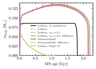
We evolve a star from the zero age main sequence (ZAMS) to the terminal age main sequence (TAMS) using the predictive mixing scheme at the convective core boundary; . Figure 1 plots the mass coordinate of the convective-core boundary as a function of MS age, showing results from separate runs using Schwarzschild and Ledoux criteria, and additional runs with the incremental inclusion of semi-convection (in just the Ledoux case) and then element diffusion (in both cases). For comparison, the figure also shows the outcome of using the Ledoux criterion but no predictive mixing; in contrast to the other cases which broadly agree with one another, the core growth is inhibited and the H-burning lifetime correspondingly truncated.
Note that in Figure 13 of Paper II the results obtained with the Ledoux criterion show a shrinking convective core; this behavior was due to a separate problem arising from over-smoothing of the composition gradient (see Moore & Garaud, 2016) and has since been rectified in MESA. For completeness, we include this case in Figure 1.
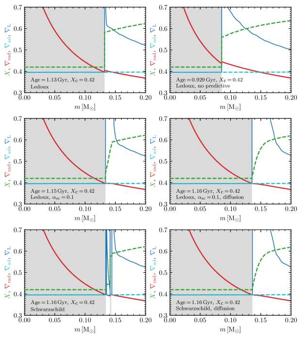
Figure 2 plots the profiles of , , and , in the inner part of the star nearing the halfway point of its MS evolution (a core H mass fraction ). In the upper row, the left panel illustrates the run with the Ledoux criterion plus predictive mixing (the dotted curve in Figure 1), while the right panel shows the run with the Ledoux criterion but without predictive mixing (the black curve, ibid.). Clearly, without predictive mixing remains significantly larger than on the convective side of the boundary, which as discussed previously is physically inconsistent. When using predictive mixing, however, the profiles satisfy on the convective side, and closely match those seen in the left panel in Figure 6 of Gabriel et al. (2014). The small bump in just above the boundary is Schwarzschild unstable but Ledoux stable.
The middle panels of Figure 2 show the runs with the Ledoux criterion and predictive mixing, and the incremental addition of semi-convection (left) and then element diffusion (right). Inside the core boundary, the profiles are almost identical to those shown in the upper-left panel but just outside the boundary, the semi-convection converts the composition discontinuity into a steep gradient and flattens the bump in to a neutral, profile. Element diffusion further softens the abundance profile, as shown in the middle-right panel. Note that element diffusion has only a small effect on the location of the convective boundary; this is barely noticeable in Figure 2, but a slight extension of the boundary can be seen in Figure 1 toward the later part of the MS, for the two cases including diffusion.
The lower panels of Figure 2 show the runs using the Schwarzschild criterion and predictive mixing, without (left) and with (right) element diffusion. In the left panel, the abundance profile shows a chaotic staircase-like profile, due to mixing by transient convective shells that appear and disappear from one timestep to the next (two of these shells can be seen in the figure). The shells do not appear in the Ledoux plots (middle and upper panels) because the region outside the core is stabilized in its entirety by the abundance gradient: . This serves as a good illustration of the earlier discussion (Section 2.1) of how the Schwarzschild and Ledoux criteria can sometimes lead to different outcomes. It is important to note, however, that the location of the core boundary is the same in all cases with predictive mixing; the differences only appear in the inhomogeneous region beyond the boundary which arises from slow H burning outside the core.
The lower-right panel of Figure 2 shows that adding element diffusion removes the abundance discontinuities, replacing them with a smooth gradient. The resulting profiles appear almost identical to the Ledoux case shown in the middle-right panel of the figure (and compare also the curves with diffusion in Figure 1).
2.3 Evolution of a Retreating Convective Core on the Main Sequence
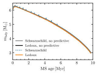
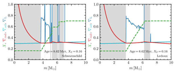
We now evolve a star from ZAMS to TAMS using the new predictive mixing scheme at the convective core boundary; . Figure 3 plots the mass of the convective core as a function of MS age, showing results from separate runs using the Schwarzschild and Ledoux criteria, and with and without predictive mixing. The agreement between these four cases is very close. However, as was the case in the preceding section, there are differences outside the convective core. These can be seen in Figure 4, which plots the profiles of , , and near the end of the star’s MS evolution (), for the two runs with predictive mixing.
Even though both runs exhibit the same core structure, with at the convective side of the core boundary, the inhomogeneous region left behind by the retreating core is very different. The H abundance obtained with the Schwarzschild criterion shows the same staircase-like profile seen in the lower-left panel of Figure 2, again due to mixing by transient convective shells. These shells are not present when the Ledoux criterion is used, with the exception of a persistent solitary shell at the top of the inhomogeneous region (corresponding to where the core boundary was located at the ZAMS); the behavior of this shell is discussed by Gabriel et al. (2014, their Section 5.5.1; and compare also against their Figure 4). Between the shell and the core boundary, the abundance profile from the Ledoux run remains relatively smooth. The different abundance profiles in the two runs will have a direct influence on the Brunt-Väisälä frequency profile, and therefore on the oscillation frequencies of the stellar model.
2.4 Evolution of the Convective Core during Core He Burning
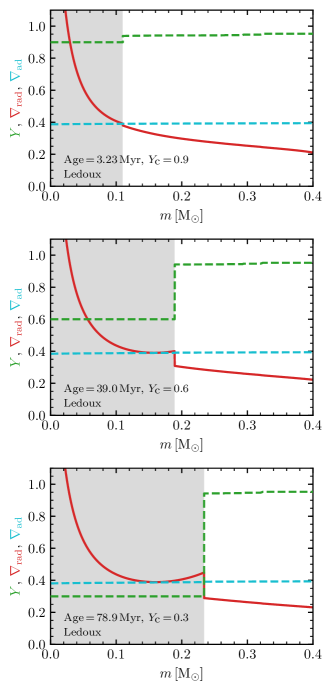
As reviewed by Salaris & Cassisi (2017), the modeling of mixing in low- and intermediate-mass stars during core He burning (CHeB) is particularly challenging. Correct treatment of convective boundaries is complicated by the fact that the profile within the core convection region develops a local minimum at some point during CHeB evolution (see the middle and lower panels of Figure 6). This is a consequence of the complex behavior of the physical quantities (opacity, temperature, density, etc.) involved in the expression for . With further outward propagation of the convective boundary, the mixing of fresh He into the core can lower the radiative gradient throughout the core to such an extent that at the local minimum of . When this happens, the part of the convection region interior to the minimum becomes decoupled from the part exterior to the minimum: the convection region has split. This phenomenon was first discussed by Eggleton (1972)
Another problem appears near the end of CHeB. At that point, even small amounts of He added to the core (which is almost totally depleted in He) will enhance the rate of energy production and thus the luminosity, resulting in an increase in . This increase leads to a sudden growth in the core boundary and a “breathing pulse”. The He is then quickly burned in the core and the star re-adjusts itself. The existence of these breathing pulses remains controversial and it is still unclear whether they are numerical or physical (Caputo et al., 1989; Cassisi et al., 2003; Farmer et al., 2016; Constantino et al., 2017). All of these problems are clearly described and illustrated in Salaris & Cassisi (2017).
To manage these complexities, the predictive mixing scheme must be modified. When a convection region splits, it is no longer meaningful to re-evaluate using opacities and other data calculated on the assumption of uniform composition throughout (Section 2.1), because the radiative region appearing at the split point prevents the free exchange of material between the adjacent convection regions. Although in principle we could resort to the partial mixing mentioned above, in practice it is not clear how this might be implemented within a diffusive mixing framework. Constantino et al. (2015) have developed an overshoot-like prescription which appears useful for mimicking the convective neutrality achieved by partial mixing (see their Section 2.3.3), but it involves a number of unconstrained parameters. Therefore, on grounds of simplicity and pragmatism — and recognizing that better approaches may become apparent in the future — we modify the predictive scheme to prevent it from causing a convection region to split in the first place. This involves a new control parameter, predictive_superad_thresh; if during the predictive mixing iterations the super-adiabaticity drops below this threshold anywhere in the mixed region, then the code backs off the mixing by one cell and updates the model convective diffusivities and convective velocities in the usual manner.
Further functionality, controlled by a new parameter predictive_avoid_reversal, also helps to prevent splitting and breathing pulses. When this parameter is set to the name of a MESA isotope, then the code monitors how the predictive mixing alters the abundance evolution of that isotope in the convection region. If it would cause this evolution to reverse (i.e., switch from decreasing to increasing, or vice-versa), then the code backs off the mixing by one cell and updates the model as before. Thus, for instance, setting this parameter to ‘he4’ during CHeB ensures that the predictive mixing scheme does not cause the core He abundance to increase across a timestep.
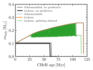
To illustrate the preceding discussion, we evolve a star through CHeB; this is the same mass considered by Constantino et al. (2015). Figure 5 plots the mass of the convective core as a function of CHeB age (defined as the time elapsed since the central drops below 0.98), showing results from separate runs with and without predictive mixing, and using the Schwarzschild and Ledoux criteria. For the cases with predictive mixing, we adopt a value of 0.005 for the predictive_superad_thresh parameter, and set predictive_avoid_reversal to ‘he4’ to prevent any reversal in the core He abundance. Figure 5 also shows the results from an additional Ledoux/predictive mixing run where we allow the core to split by not setting the predictive_avoid_reversal and predictive_superad_thresh controls.
Figure 5 shows that without predictive mixing the core is prevented from growing, and the CHeB lifetime significantly curtailed, irrespective of whether the Schwarzschild or Ledoux criteria are used (see also Figure 15 of Paper II). With predictive mixing but no splitting allowed, however, the core grows steadily until He is exhausted, and no breathing pulses are seen. There is almost no difference between the Schwarzschild and Ledoux cases. When the core is allowed to split, the evolution is much noisier. Starting at an age , the core undergoes episodes of splitting and rejoining that repeat on a short timescale. Toward the end of the evolution, as the core helium abundance becomes very small, the timescale between successive splittings becomes longer, until the core finally splits without rejoining. The overall CHeB lifetime of the model is shortened by relative to the cases where splitting is avoided.
Figure 6 plots the profiles of , and for the star at three points during its CHeB evolution, corresponding to core helium mass fractions , 0.6 and 0.3. The profiles are all from the run with the Ledoux criterion and predictive mixing. In the upper panel, a local minimum in has yet to develop, and the core boundary satisfies the equality on its convective side. In the middle and lower panels, the local minimum in can clearly be seen; in these cases, the predictive mixing has extended the convection region as far as possible without pushing the minimum below the threshold set by the predictive_superad_thresh control. MESA treats the region between the minimum and the convective boundary as fully convective. On the convective side of this boundary , which is physically inconsistent but cannot be remedied with predictive mixing alone: any further extension of the boundary would cause the convection region to split. As discussed above, fixing this inconsistency requires some way of modeling the partial mixing expected to occur in the part of the convection region between the minimum and the boundary.
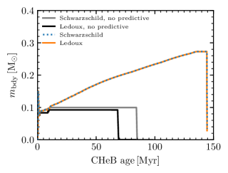
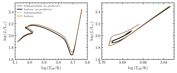
To explore whether the predictive mixing performs equally well for a higher-mass star that has not passed through the He flash, we also evolve a star through CHeB; this is the same mass and evolutionary stage considered in Figure 15 of Paper II. Figure 7 plots the mass of the convective core as a function of CHeB age, showing results from separate runs with and without predictive mixing, and using the Schwarzschild and Ledoux criteria. For the cases with predictive mixing, we again adopt a value of 0.005 for the predictive_superad_thresh parameter, and set predictive_avoid_reversal to ‘he4’ to prevent any reversal in the core He abundance. As before, we find that the predictive mixing allows the core to grow steadily; and that the Schwarzschild and Ledoux criteria give essentially the same outcome.
2.5 Evolution of the Bottom of the Surface Convective Region in a Low-Mass Star
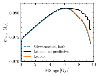
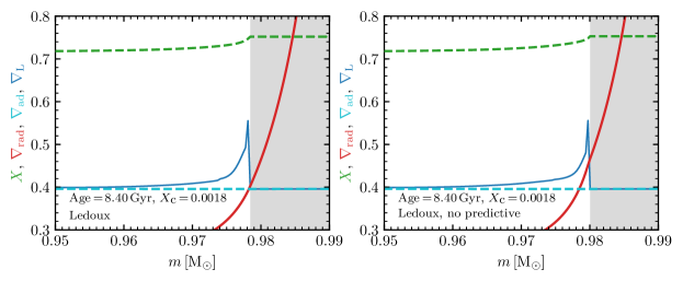
We now evolve a star from ZAMS to TAMS, using the predictive mixing scheme to position the lower boundary of the convective envelope. We include element diffusion in these calculations; when it is excluded, the composition remains completely uniform throughout the stellar envelope, and predictive mixing makes no difference whatsoever to the evolution. Figure 9 plots the mass coordinate of the convective boundary as a function of MS age, showing results from separate runs with and without predictive mixing, and using the Schwarzschild and Ledoux criteria.
The four runs are in agreement until an age 6.5 ; after this point, the downward growth of the region boundary is slower in the run that does not include predictive mixing with the Ledoux criterion. Figure 10 plots the profiles of , , and , in the outer part of the star at an age . The left panel illustrates the run with the Ledoux criterion plus predictive mixing, while the right panel shows the run with the Ledoux criterion but without predictive mixing. The former shows that on the convective (upper) side of the convective boundary, while the latter has consistent with the boundary growth being retarded.
2.6 Effect of Timesteps and Mesh Size
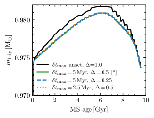
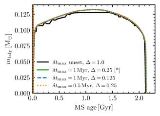
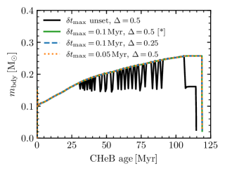
We now demonstrate how limiting the maximum timestep (set by the max_years_for_timestep control) and changing the mesh resolution parameter (set by the mesh_delta_coeff control; see Section B.4 of Paper II for further details) influences the results presented in the previous sections.
First we consider the effects of changing timestep and resolution on the position of the convective envelope boundary in the model considered in Section 2.5, focusing specifically on the case with the Ledoux criterion and predictive mixing. The results presented previously in Figure 9 are calculated using and . Figure 11 demonstrates that halving either or has little effect on these results, confirming that the calculations are converged. Such settings need to be applied when a converged result is desired from MESA for this calculation.
Figures 12 and 13 repeat this exercise for the position of the core convection boundary in the MS model and CHeB model, respectively. The results presented previously are clearly converged, and this exercise clarifies the MESA settings that should be used for this calculation.
3 Element Diffusion
Section 9 of Paper III describes in detail the old implementation of element diffusion in MESA. Section 9.3.4 points out limitations to those methods, namely: (1) electron degeneracy was not properly accounted for in the diffusion equations, and (2) strong Coulomb interaction introduced theoretical uncertainties for the diffusion coefficients. These two issues are especially important when modeling diffusion in WDs. Here we describe the impact of degeneracy and present new methods to incorporate its effects. We also discuss recent updates to diffusion coefficients and potential approaches for further improvements.
3.1 Degeneracy and the Approach in Paper III
The approach to diffusion presented in Section 9 of Paper III assumes all particles obey the ideal gas law. Electron degeneracy pressure can significantly modify the EOS and violate this assumption.
For a plasma species (i.e., electrons and ions) with partial pressure , mass density , charge density , number density , and temperature , the Burgers (1969) equations for diffusion are
| (1) | ||||
| (2) | ||||
The resistance coefficients , , , and are defined in Equation (86) of Paper III. With representing the total number of plasma species, we must solve for unknowns: diffusion velocities (), heat flow vectors (), the electric field (), and the gravitational acceleration (). The Burgers equations above for each species provide equations, so we can close the system with two additional constraints, which are no net flow of mass or electric current due to diffusion,
| (3) |
| (4) |
This gives a total of equations.
When electrons are degenerate, Equation (1) is difficult to apply since no longer takes a simple analytic form. Moreover, the temperature term appearing on the left hand side of Equation (2) clandestinely assumes an ideal gas law. Burgers (1969) defines the temperature for each species as and assumes thermal equilibrium between all species so that . The quantities and are defined in terms of moments of a Maxwellian distribution function, but the Fermi-Dirac distribution function for electrons no longer reduces to a Maxwellian form when they are degenerate, and hence . If the electrons remain in thermal equilibrium with their surroundings while failing to satisfy an ideal-gas relation for their temperature, the Burgers treatment assigns an incorrect temperature to degenerate electrons for the term in Equation (2).
Furthermore, the approach to diffusion described in Paper III follows Thoul et al. (1994) in rearranging and rescaling all equations into one matrix system with units convenient for solving numerically,
| (5) |
The sum on the left hand side skips the electron index because by construction, and so we save resources by not evaluating its gradient unnecessarily. Here, indices encode the equations given by Equation (1), indices encode the equations given by Equation (2), and indices encode the constraints of no current or mass flux. For definitions of the various coefficients and matrices in Equation (5), consult Paper III and Thoul et al. (1994). We repeat a few particularly relevant definitions here. First, let denote the species concentration, where is the electron number density. Second, define the total concentration as . Then the quantity appearing in Equation (5) above is defined as
| (6) |
The term in Equation (5) is meant to capture contributions of the driving terms in Equation (1). But this correspondence only holds if the ratio of the partial pressure for species to the total pressure is given by
| (7) |
where is the total number density. This holds as long as all pressures are ideal-gas. However, once electron degeneracy modifies the equation of state, does not scale linearly with , and so Equation (7) fails for all species in the plasma. This means the term no longer accurately represents the information in the Burgers equations for the diffusion velocity of any species.
Moreover, the prefactor in Equation (5) also assumes ideal gas for each species. The quantity simply scales out some of the information common to all diffusion coefficients in the units used for Equation (5). Thoul et al. (1994) assume an ideal gas to simplify the prefactor in Equation (5) to
| (8) |
where is the mass of species in atomic mass units. This scaling was propagated into the MESA diffusion routine described in Paper III. Since ideal gas pressure can be significantly smaller than total pressure when electrons are degenerate, this prefactor for Equation (5) is systematically too small for degenerate plasmas. This can result in diffusion velocities that are many orders of magnitude smaller than obtained by a proper solution.
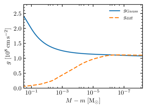
We can verify that there are problems in the degenerate regime by looking at the local gravitational acceleration , which is solved for simultaneously with the diffusion velocities in the diffusion routine described by Paper III. MESA also reports the gravitational acceleration independent of the diffusion routine, . For a MESA WD model, layers below the surface quickly become degenerate, and the difference between and is significant (Figure 14). This reflects the fact that the solutions given by the diffusion routine scale with a pressure that is far too small in the interior.
3.2 New Methods
We now describe new methods that have been introduced to avoid the limitations discussed in Section 3.1.
3.2.1 Recasting the Burgers Equations
The problems with Equation (5) demonstrated in Figure 14 can be circumvented by solving the Burgers equations directly as presented in Equations (1) and (2). When avoiding the rescaling of the Burgers equations that was originally adopted from Thoul et al. (1994), no limitations on the form of total pressure are present.
To that end, we recast the diffusion solver into the form given in Appendix C. This form closely follows the general approach presented by Thoul et al. (1994) for arranging the full set of equations into a single matrix equation, but enters the Burgers equations into that matrix structure without rescaling any quantities. We therefore avoid making any additional ideal-gas assumptions beyond those already present in the Burgers equations.
3.2.2 Resolving the Degeneracy Problem
Electron degeneracy makes it difficult to evaluate the term in Equation (1) in the case of electrons, but it is possible to form a closed set of diffusion equations that makes no explicit reference to this equation for the electrons. Even in many applications involving WDs, each ion species can be treated as approximately ideal, and hence Equation (1) remains useful for ions. We are then left with just two problematic equations out of the system of equations: Equations (1) and (2) for the electrons.
For the species of ions in the system, we can write Equations (1) in the form
| (9) | ||||
where is the average charge of species obtained using Paquette et al. (1986b). Taking this together with Equations (2) and the two constraints on current and mass flux, we have a total of equations. If we drop as an unknown and treat it as a fixed input to the diffusion routine in MESA using , we are left with unknowns. This gives a closed system of diffusion equations with no explicit reference to the problematic Equation (1) for electrons. This is the form of diffusion equations described in Appendix C.
The thermal diffusion terms (those including in Equation 2) still contain ideal-gas assumptions as described in Section 3.1. Fortunately, in WD cores where strong electron degeneracy occurs, electron conduction leads to efficient thermal transport, resulting in small temperature gradients. With , where is the local scale height, the heat flow vectors (representing kinetic energy carried along a temperature gradient by diffusing particles) become negligible: for all . Thus for WD interiors the system of diffusion equations can be simplified by dropping the heat flow terms, removing the need for the Equations (2). Indeed, according to Iben & MacDonald (1985) and Paquette et al. (1986b), thermal diffusion leads only to small corrections to the diffusion velocities for degenerate WD interiors.
Therefore, following Iben & MacDonald (1985), we provide options for neglecting thermal diffusion in electron degenerate regions, setting and dropping Equation (2) for each species. Equation (LABEL:eq:BurgersMomentum) then simplifies to the following equations that no longer depend on for the ions:
| (10) | ||||
which matches Equation (10) from Iben & MacDonald (1985). Together with the constraints, this leaves a simplified set of equations for unknowns: diffusion velocities and the electric field .
Thermal diffusion terms tend to enhance gravitational settling velocities (Iben et al., 1992). This can be seen in Figure 15 for a star on the MS, where the solvers that include thermal diffusion speed the sedimentation of away from the surface relative to the solver that neglects thermal diffusion. MESA also provides options for smoothly transitioning between diffusion velocities obtained with and without thermal diffusion (averaging between the two solutions in a blending region as a function of electron degeneracy parameter). By default, this transition region occurs when the electron chemical potential is near , but it is left to the user to decide on an appropriate range of electron degeneracy over which thermal diffusion should be shut off, if at all. The effect of blending between solvers with and without thermal diffusion is to suppress the thermal enhancements to diffusion velocities, smoothly pushing the enhancements to zero as electrons reach a degeneracy threshold. The implementation for the simplified set of diffusion Equations (10) and the smooth turn-off of thermal diffusion terms as a function of degeneracy are described in Appendix C.
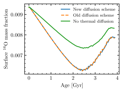
In order to confirm that we recover the correct behavior on the MS, we compare results obtained with different diffusion routines for a star in Figure 15. Here the results based on Thoul et al. (1994) are valid, since no significant departures from ideal-gas behavior are present near the surface. The results obtained with the new scheme are in agreement.
3.2.3 Diffusive Equilibrium
Paper II and Paper III show abundance profiles for WDs that have reached diffusive equilibrium in their outer layers. Figure 23 of Paper II compares the diffusive tails of H and He to an analytic expression from Althaus et al. (2003) and finds good agreement. However, Althaus et al. (2003) note that their analytic expression for diffusive equilibrium follows Arcoragi & Fontaine (1980) in assuming an ideal gas, and the equilibrium abundance profiles from their evolutionary models deviate from the analytic expression due to the inclusion of electron degeneracy. Similarly, the He layer of the WD model shown in Figure 43 of Paper III is partially degenerate, and hence the driving forces for diffusion should be modified in this region.
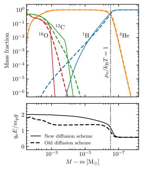
For a fully-ionized isothermal ideal gas the electric field that serves as one of the driving forces for diffusion in Equation (LABEL:eq:BurgersMomentum) takes the form . In contrast, in the limit of strong electron degeneracy, the electric field approaches . When He is the background material, the electric-to-gravitational force ratio increases from to . In this limit, any trace isotopes with see no net sedimentation force (), while H with sees a significant upward sedimentation force (). This extra buoyant force on H in a degenerate He background pushes the diffusive tail further toward the surface relative to the ideal-gas case, as shown in Figure 16. With the proper handling of electron degeneracy described in Section 3.2, our MESA models now agree with the time-dependent diffusion models shown in Figure 18 of Althaus et al. (2003).
3.2.4 Radiative Levitation
Radiative levitation is included as an optional extra term. The Burgers equations are modified with a extra forcing term by taking , as shown in Equation (99) of Paper III. Our implementation continues to follow Hu et al. (2011) but no longer employs their matrix structure for the Burgers equations; details of how the terms are handled with the updated diffusion schemes can be found in Appendix C.
3.3 Updated Diffusion Coefficients
The Paquette et al. (1986a) diffusion coefficients have served as the standard for stellar diffusion problems. The scattering cross-sections for these coefficients are calculated using a screened Coulomb potential
| (11) |
with the screening length chosen as , where is the Debye length, is the average interionic distance, and is the ion density. This choice is a crude but effective way to handle the strongly coupled regime; as shown in Paper III, this yields reasonable agreement with diffusion coefficients calculated from molecular dynamics.
Stanton & Murillo (2016) provide updated calculations of collision integrals for screened Coulomb interactions and suggest improvements to the treatment of screening length. They provide fitting functions and tables that can be used with any choice of screening length. In MESA we follow their suggested screening prescription. The electron screening length is given by a Thomas-Fermi approximation that accounts for non-relativistic degeneracy:
| (12) |
where is the electron Fermi energy. The direct inclusion of degeneracy increases . The ion screening lengths are the Debye lengths for each species,
| (13) |
To prevent ions from screening below the inter-ionic spacing, Stanton & Murillo (2016) introduce an approximate ion-sphere for each species , and define an ion-sphere coupling parameter
| (14) |
Their net effective screening length is then
| (15) |
This construction enforces a minimum on the screening length at approximately the ion-sphere radius for each species, similar to the strict minimum at set by Paquette et al. (1986a). Stanton & Murillo (2016) point out that this adjustment to the ion screening length is physically motivated by the ion pair distribution functions in a strongly coupled plasma, where the occupation probability within the ion-sphere radius is negligible, and hence no ions are present to provide screening beneath that cutoff. The proper handling of degeneracy in the electron screening length makes it unnecessary to impose any particular minimum there, so there is no longer any ad hoc appeal to a universal minimum screening length.
For repulsive Coulomb potentials of the form in Equation (11), Stanton & Murillo (2016) provide fits and tables of collision integrals and coefficients that we now use to calculate the resistance coefficients for inclusion in the Burgers equations in MESA. They do not provide fits for attractive potentials, and Paquette et al. (1986a) note that interactions with these potentials behave significantly differently from those with repulsive potentials when screened. Hence, MESA continues to use the Paquette et al. (1986a) coefficients for electron-ion terms, and adopts Stanton & Murillo (2016) for all ion-ion coefficients. In any case, it is evident from Equation (94) in Paper III that the resistance coefficients approximately follow , where is the reduced mass of particles and ; so, electron-ion resistance coefficients are generally negligible compared to the ion-ion terms.
The calculations of Paquette et al. (1986a) overestimate the electron-ion resistance coefficients in the case where electrons are degenerate. This is because diffusion and resistance coefficients are generally calculated assuming that the velocity distributions of all particles are Maxwellian, and the coefficients roughly scale as . When the electrons become degenerate, their characteristic kinetic energies are of order , and so their velocity distribution skews toward larger velocities. This results in smaller resistance coefficients , overestimating the impact of electron-ion drag. However, the overestimate results in coefficients that remain negligible compared to ion-ion terms, and no attempt is made to correct it in MESA.
For repulsive potentials, the coefficients from Stanton & Murillo (2016) generally agree with those of Paquette et al. (1986a) to within a few percent. In strongly coupled WD interiors the Stanton & Murillo (2016) coefficients lead to shorter diffusion timescales due to a screening length that is allowed to be somewhat smaller than the minimum value imposed by Paquette et al. (1986a): . Future prospects for further improvements to diffusion coefficients include the recent progress on effective potential methods from Daligault et al. (2016) and Shaffer et al. (2017).
3.4 Diffusion-Induced Flashes on He WDs
Diffusion-induced H shell flashes on low-mass () He WDs are known to alter their cooling times (Althaus & Benvenuto, 2000; Althaus et al., 2001) and seismic properties (Althaus et al., 2013). Istrate et al. (2016a, b) use MESA to model this process, generating tables of cooling timescales and comparing MESA models with those of Althaus et al. (2013).
Figure 17 shows an exploration of the H shell flash domain for a large grid of MESA models over a range of He-core and H-envelope masses. Here the envelope mass is defined as the total mass of H-rich material () at the surface at the beginning of the WD cooling track. Lines show the minimum envelope masses for which H shell flashes occur given various diffusion prescriptions.
For a given core mass, there is a range of envelope masses that exhibit shell flashes only if diffusion is included, but this range depends on the diffusion prescription. The two lower lines for models including diffusion in Figure 17 differ only in the handling of electron degeneracy in the diffusion scheme. This illustrates the importance of properly handling degeneracy as described in Section 3.2, since the diffusion-induced flashes are typically ignited by CNO burning in the diffusive tail of H that reaches into the partially degenerate He layers. WDs in this mass range often experience cycles of many H flashes, depleting H incrementally until insufficient H remains to ignite another flash. The disagreement between diffusion prescriptions on the minimum envelope mass for flashes is therefore significant, as this will determine the total number of flashes and final H mass that sets the ultimate cooling timescale for an object.
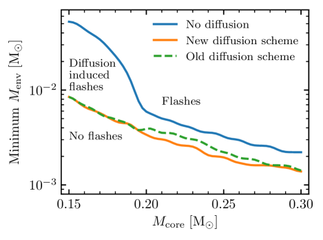
To explore the full range of parameters presented in Figure 17, our WD models were built by artificially stripping the H envelope down to a specific mass coordinate above the He core of a model ascending the RGB. For a discussion of MESA models including proto-WD formation and the resulting H envelope masses, see Istrate et al. (2016b).
3.5 Heating from Settling
In the strongly degenerate limit, for C/O WD cores. For an isotope where , the electric and gravitational fields result in a net force that drives diffusion. For in cooling WD interiors, this force is , causing to sediment toward the center and deposit energy as it moves deeper into the gravitational potential (Bildsten & Hall, 2001; Deloye & Bildsten, 2002; García-Berro et al., 2008, 2010). This heating can prolong the WD cooling timescale, especially at late times when the WD is very dim and radiates away the energy slowly. This effect may be especially important for explaining WD luminosity functions in old and metal-rich open clusters such as NGC 6791, where abundant is available in WD interiors to provide heating.
MESA now offers an option to include this heating term in the energy equation (see Section 8.7) when diffusion is enabled. The specific rate at which energy is deposited is
| (16) |
The diffusion velocity () and electric field are calculated in the diffusion routine and then used to evaluate the above heating term. Note that the updates to diffusion described in Section 3.2 are essential for correctly calculating both the diffusion velocity and magnitude of the driving force in the degenerate interior of the WD.
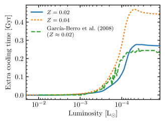
Figure 18 shows the delay in WD cooling from introducing into models. These models turn off diffusion for , so is only active in material for which crystallization has not yet occurred. The time-delays shown in Figure 18 are in good agreement with those shown by Deloye & Bildsten (2002) and García-Berro et al. (2008) for comparable cases.
4 Implicit Hydrodynamics
In Paper III we describe implicit shock-capturing hydrodynamics capabilities based on the use of an artificial viscosity. We now add an option for using an approximate Riemann solver, the HLLC (Harten-Lax-van Leer-Contact) solver introduced by Toro et al. (1994). (See also Batten et al. 1997 for an early implicit implementation of HLLC.) The HLLC method provides improved shock capturing and energy conservation by avoiding the need for artificial viscosity. However, the methods presented in Paper III are still included in MESA so that users may continue to apply them.
4.1 Implementation of HLLC
Accurate shock-capturing methods evaluate the flux of hydrodynamical conserved quantities by extrapolating the solution on each interface between zones over the course of the timestep. The different methods for projecting the solution into the future are known as different “Riemann solvers”. HLLC is designed to accurately capture the evolution of contact discontinuities. When implemented on a Lagrangian grid, HLLC is able to evolve purely advective flows without any contact smearing (Cheng & Shu, 2007; Duffell & MacFadyen, 2011; Cheng et al., 2012; Cheng & Shu, 2014).
Paper I and Paper III discussed the evolution of a velocity variable , defined at cell faces. When using HLLC, MESA instead evolves a cell-centered velocity .
We solve a Riemann problem at the cell face with index . The cell to the left (toward the center) is the cell with index ; the cell to the right (toward the surface) is the cell with index . The cell face radius is . The mass contained within an individual cell is . The mass enclosed from the center of the star to the cell face is . For convenience, we define the face area as . Thermodynamic variables (e.g., , ) are defined at cell centers by mass. Figure 19 shows the layout of cells.
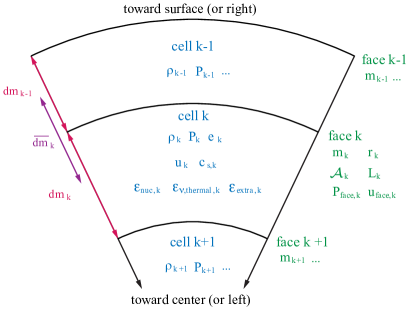
The calculation begins by making estimates for the density and velocity at the left and right of the face. Explicit codes sometimes use multipoint polynomial interpolation based on values in neighboring cells to improve the reconstruction of the values at the face. However for an implicit code such as MESA, that would introduce dependencies in the partial derivatives for the Jacobian that would violate the necessary block tridiagonal structure (see Appendix B in Paper II). To avoid this problem, we use the cell center density and velocity alone to estimate the values at the edges of that cell. The variables for the left and right values are named relative to the edge rather than the cell, that is
| (17) | ||||||
This choice limits the solution to be first-order accurate in space.
Using an approach similar to Käppeli & Mishra (2014), we reconstruct the pressure at the faces assuming hydrostatic equilibrium. The pressure derivative implied by hydrostatic equilibrium at the face is
| (18) |
and we reconstruct the pressure to the left and right of the face
| (19) | ||||
This choice improves the timescale over which hydrostatic equilibrium can be maintained when using HLLC, and facilitates the process of switching from a hydrostatic model to one in which a velocity variable is evolved.
The 1D Lagrangian context makes the implementation of HLLC straightforward. In a Lagrangian code like MESA there is no mass flux across cell faces. In hydrodynamics, there is no mass flux across a contact discontinuity. HLLC includes the contact wave, so we simply associate the contact wave with the cell face.111In Section 5, where we consider the effects of mass diffusion, we will need to slightly revise this association. As given by Toro (2009), the HLLC estimate of the contact wave speed is
| (20) |
and hence =. Likewise, the pressure at the cell face is the pressure at the contact wave, =, where
| (21) |
and and are the fastest wavespeeds moving to the left and right, respectively. To evaluate these, we assume the simple and most conservative bounds on the signal velocities,
| (22) |
where and are the sound speeds on the left and right sides of the cell boundary, respectively. Having obtained values for and , we now formulate the versions of the equations used when HLLC is enabled.
In the Lagrangian picture, the cell boundaries move with the fluid velocity, such that the net fluxes for mass, momentum, and energy from cell to cell are extremely simple (Cheng & Shu, 2014) and given by
| (23) |
The term in the energy flux does not come from the solution of the Riemann problem, but from the fact that MESA also evolves a luminosity variable that reflects the radiative or convective transport of energy.
The finite volume form of the mass conservation equation remains the same as that given in Paper I,
| (24) |
However, the equation for the radius (Equation 29 in Paper III) has changed. The new equation for the radius is
| (25) |
where is the timestep. For numerical precision, we re-write this as
| (26) |
where this recasting allows use of crlibm (de Dinechin et al., 2007, see also Paper III) function expm to evaluate the function to machine precision (as indicated by the underbrace).
The local radial momentum equation for cell is
| (27) |
On the right hand side, the first term is gravitational, the second is a geometric source term that arises from putting the equation in conservation-law form, and the final term is the momentum flux in and out of the cell found by HLLC.
The local total energy conservation equation for cell is
| (28) |
(See Section 8.3 for a discussion of how this energy accounting is related to that typically used in stellar evolution calculations.) We define the cell center quantities and to be and at the center of mass of the cell. The terms on the left split the local total energy into internal, kinetic, and potential components. The right side gives the energy in and out of the cell and the energy sources and sinks in the cell. Energy loss from neutrinos due to nuclear reactions is already subtracted from the nuclear burning term, , so only the neutrino energy loss rate from thermal processes, , is explicitly accounted for in Equation (28). Other processes are accounted for via .
As in Paper I, the temperature differences of interior cells are set by energy transport across boundaries,
| (29) |
where is provided by MESA module mlt (see Section 5.1 in Paper I) and the overbars indicate quantities at the cell faces (see Figure 19). This equation relates temperatures of neighboring cells; the actual temperature in each cell is then fixed by a surface boundary condition.
MESA’s HLLC includes the effects of rotation in the shellular approximation (see Paper II, Section 6.1) and can also include a post-Newtonian correction to the gravitational force. (For an example application to neutron star envelopes, see Paper III, Section 5.3). These capabilities require modifications to the momentum equation. In both cases, they can be treated as a rescaling of the local gravitational constant . In the case of rotation, the rescaling factor is (Paper II, Equation 23). In the post-Newtonian case, it is . Therefore, when either of these is used with the hydrodynamics capabilities described in this section, the rescaling is applied to the in pressure reconstruction (Equation 18) and separately to each (for cell and ) in the momentum equation (Equation 27).
4.2 Mesh Refinement
During a typical stellar evolution run, MESA controls its meshing using “mesh functions” that limit the maximum allowed change of various quantities between adjacent cells (see Section 6.5 in Paper I and Section B.4 in Paper II). With HLLC, the criteria to split or merge cells are written solely in terms of the radial coordinate in order to simplify the adjustments to the mesh in response to large changes in density before and after a shock. Cells split when they decompress enough that their radial extent becomes too large, and they merge with a neighbor when they compress enough that their radial extent becomes too small.
The refinement criteria can use either linear (=) or logarithmic (=) radius. The user selects a target number of cells, . MESA translates this into a target cell size, =. A cell is considered too large if and a cell is considered too small if .222By default , and , but these parameters are configurable at run-time. The refinement then proceeds iteratively. At each iteration, MESA selects the smallest and largest cells. If the largest cell is too large, it is split. If the smallest cell is too small, it is merged unless the magnitude of the difference between its velocity and that of either neighbor is a significant fraction of the local sound speed: this prevents merging in the immediate vicinity of the shock where there are sharp jumps in velocity. The refinement proceeds up to some maximum number of iterations, though in practice the procedure typically stops before then because no more cells satisfy the criteria to be split or merged.
A cell merges with its smaller neighbor, unless they have a different most-abundant chemical species, in which case the cell merges with the other neighbor instead. When a cell is split, differences in quantities such as density and chemical abundances between the two child cells are determined by interpolation from the neighboring cells.
4.3 Time Resolution
Since the hydrodynamics equations are being solved implicitly, MESA is not subject to the Courant-Friedrichs-Lewy (CFL) timestep condition for numerical stability. The size of the MESA timestep is instead limited by the restrictions on the allowed changes in the structure of the star. The usual timestep controls continue to apply.
While numerical stability does not require the restrictive CFL timestep condition, the choice of timestep does affect the accuracy of the solution. A CFL-like limit is often also applied because it can be a convenient additional way to restrict timesteps along with the other options. Such a restriction allows for well-converged solutions. The timestep can be limited by the requirement that
| (30) |
where is a user parameter. Unlike in an explicit code where a similar minimum must be evaluated over all cells, in MESA the minimum is taken only over cells for which
| (31) |
where is the maximum evaluated over nearby cells, and is a user parameter.333The value of is similar to the values of a CFL parameter in an explicit code, while in the examples is typically a small value like . The description of these limits is schematic and the reader is referred to the source code for the precise implementation details. This means that only regions near the shock front limit the timestep. The option for additional limitations on where this condition is evaluated (e.g., in mass) are provided.
4.4 Hydrodynamic Test Problems
In order to test the HLLC implementation, comparisons are now made to problems with known solutions.
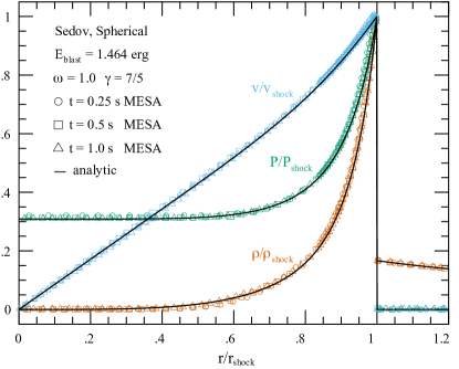
4.4.1 Sedov Blast Wave
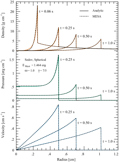
In the Sedov blast wave problem, an energy is deposited at the origin at time zero in a domain with a non-uniform density profile , where and are constants. We assume an ideal-gas EOS with a constant adiabatic index , that is .
Generation of numerical Sedov solutions is discussed in Kamm & Timmes (2007). A constant initial density profile, =0, is frequently used in verification tests (e.g., Gehmeyr & Mihalas, 1994; Fryxell et al., 2000). Although a power-law initial density profile is more challenging for verification studies, we explore such a profile because density gradients are prevalent in astrophysics.
To model a shock propagating down a linear density gradient in spherical geometry we set =1, =7/5, =1 g cm-3, and =0 erg cm-3 in the analytic solution; while we set =10-6 erg cm-3 in MESA as a stable numerical approximation to zero pressure. The initial blast energy, =1.464 erg, is determined by choosing that =1 cm at =1 s and then calculating the Sedov energy integral. Figure 20 shows the evolution of the density, pressure, and velocity. As the shock propagates outward from the origin these quantities monotonically decrease as mass is swept up by the shock. The spherical Sedov problem admits a similarity solution. Figure 21 demonstrates that MESA maintains the analytic self-similar profiles at different times.
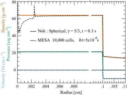
4.4.2 Noh Problem
Noh (1987) describes a standard verification problem that tests the ability to transform kinetic energy into internal energy, and the ability to follow supersonic flows. A sphere of cold gas with an ideal-gas EOS and constant adiabatic index , that is , is initialized with a uniform, radially inward speed of 1 cm s-1. A shock forms at the origin and propagates outward as the gas stagnates. For an initial gas density =1 g cm-3, the analytic solution in spherical geometry for =5/3 predicts a density 64 g cm-3 in the stagnated gas.
Figure 22 shows the analytic and MESA profiles for the density, pressure, and material speed at =0.3 s. Most implementations, including MESA’s, produce anomalous “wall-heating” near the origin (although see Gehmeyr et al., 1997). As the shock forms at the origin the momentum equation tries to establish the correct pressure level. However, numerical dissipation generates additional entropy. The density near the origin drops below the correct value to compensate for the excess internal energy (e.g., Noh, 1987; Rider, 2000). Thus, the density profile is altered near the origin while the pressure profile remains at the correct constant level in the post-shock region.
Figure 22 shows the analytic solution and MESA solution for a fixed timestep of =510-6 s and 10,000 cells. Deviations from the analytic solutions are 1%, except for the density near the origin and the shock front. A convergence exercise with different fixed timesteps and spatial resolutions suggests spatial resolution is relatively more important in the MESA solutions than temporal resolution for the Noh problem.
4.4.3 Supernova Shock
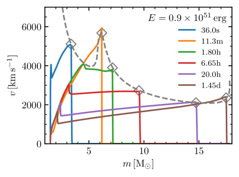
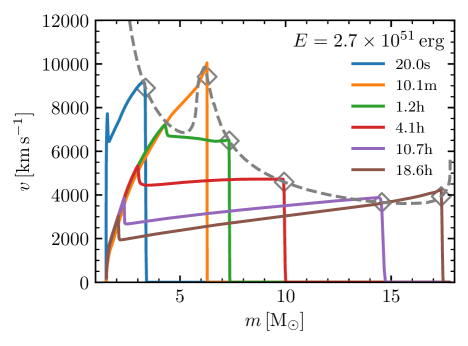
The problem of a supernova (SN) shock moving through a stellar envelope has been extensively studied. For a radiation-dominated strong shock, a simple analytic expression for the shock velocity is provided by Matzner & McKee (1999),
| (32) |
where we adopt as suggested by Tan et al. (2001). The explosion has an energy . The mass that enters into this expression is the mass entrained by the shock and so differs from the Lagrangian mass coordinate () by the mass of the remnant (). Since the material in the shocked envelope has an adiabatic index of , the Matzner & McKee (1999) prediction for the post-shock velocity is .
MESA defines the shock location to be the outermost point where the fluid Mach number exceeds 1, as measured in the rest frame of the star. Since the primary application of these capabilities are blast waves propagating into approximately static stellar envelopes, this shock detection criterion suffices. Figure 23 compares the velocity in a MESA model (the 19 model of SN1999em; see Section 6) with . We show explosions with two different energies, and . Both cases have . Typical differences are at the few percent level.
4.4.4 Weak Shock Propagation
We now explore weak shocks with Mach numbers propagating outward in the hot stellar envelope of a classical nova progenitor. The model is a WD. The H/He envelope extends from cm to cm with densities g cm-3 and temperatures K.
After excising the core we run the model with HLLC enabled for 100 s, corresponding to 50 sound crossing times in the outer envelope, to allow the envelope to settle. Afterwards, the envelope has a total energy of , with in potential energy, in thermal energy, and a negligible kinetic energy . We turn off convective energy transport to study the properties of weak shocks. To create weak shocks, we inject of the total thermal energy into a single cell with mass g at cm over s. Figure 24 shows the resulting upward and downward propagating shocks. We restrict our region of study to the region where the upward and downward shocks are well-separated, in the radius range of cm (denoted with thin gray lines in Figure 24). We do not study the properties of the downward shock and its artificial reflection from the “floor” of our model.
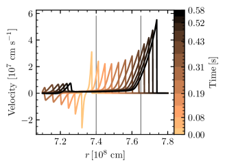
We define as the shock velocity, where is defined as the radial location with maximum fluid velocity. We compare the properties of the shock to analytic expectations for cases where is identical in the pre- and post-shock material. Pre-shocked quantities carry a 0 subscript, and shocked quantities carry a 1, and we use the sound speeds, , and pressures, , on either side of the discontinuity. Following Zel’dovich & Raizer (1967), in the rest frame of the shock front, the pre-shock gas travels into the shock front at velocity
| (33) |
The post-shock velocity has magnitude , where denotes the fluid velocity at . The analytic expression is
| (34) |
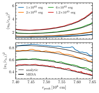
Local shocked quantities are evaluated at the cell with the maximum Lagrangian fluid velocity, while pre-shocked quantities are evaluated at the cell in the initial MESA profile (before the shock has propagated) with the same mass coordinate as the shock front when it reaches . The thin black lines in the upper and lower panels of Figure 25 are the right-hand side of Equations (33) and (34), respectively, for shocks produced by different amounts of injected energy. Colored lines show the left-hand side of each equation as calculated from the MESA model.
We now compare the temperatures and of the pre- and post-shock gas. We expect
| (35) |
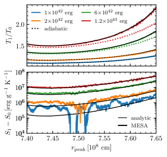
The thin black lines in the upper panel of Figure 26 show the right hand side of Equation (36) and the solid colored lines correspond to quantities calculated by MESA. The colored dotted lines in the top plot show the temperature change for an adiabatic compression,
| (36) |
making it clear that for the weakest shocks, the temperature jump is that expected from an adiabatic compression. However, for stronger shocks, the temperature is higher due to the entropy increase associated with the shock. For a gas with specific heat capacity , this entropy jump is
| (37) |
shown by the thin black lines in the bottom plot of Figure 26. The colored lines correspond to quantities calculated by MESA. The agreement is excellent for large entropy jumps, but becomes noisy at lower injection energies because extracting small changes from the background is then challenging. For the weakest shock, the entropy changes are orders of magnitude smaller than the background entropy erg g-1 K-1 in the region of interest.
5 Rayleigh-Taylor Instabilities
The outward moving shock in a core collapse SN explosion encounters multiple composition boundaries. Across these boundaries the density gradient is steep, especially at the H/He boundary. Post-shock, these regions become unstable to the Rayleigh-Taylor instability (RTI). Early analytics and 2D simulations (Chevalier, 1976; Chevalier & Klein, 1978; Weaver & Woosley, 1980; Benz & Thielemann, 1990; Herant & Benz, 1991) and modern 3D calculations (Hammer et al., 2010; Wongwathanarat et al., 2015; Utrobin et al., 2017) show significant impact on the density, velocity, and composition structure of the ejecta.
It has been known for decades that the resulting compositional mixing can significantly alter the photometry of the SN. This effect has been roughly included in 1D modeling of Type IIP light curves resulting from explosions deep within a red supergiant (Eastman & Pinto, 1993; Utrobin, 2007; Dessart & Hillier, 2010, 2011). The mass densities and energy densities are also smeared out by the mixing from the RTI (see Bersten et al. 2011 for an early discussion raising this concern). In their recent modeling of the Type IIP SN 1999em, Utrobin et al. (2017) capture the impact of the RTI using a 3D model pre-breakout and connect to observable SN properties with a 1D post-breakout radiation calculation.
To approximate the 3D effects of the RTI, we implement a scheme by Duffell (2016) that modifies the 1D spherical hydrodynamics equations. This scheme has been recently applied to the specific case of core collapse SN by P. Duffell et al. (2017, in preparation) and is now implemented in MESA for use along with the HLLC scheme. In this section, we describe the MESA implementation and compare to 3D calculations of Wongwathanarat et al. (2015). The use of the resulting RTI-mixed ejecta for SN lightcurves and velocities will be discussed in Section 6.
5.1 Implementation of Duffell RTI
The Duffell (2016) scheme evolves an additional scalar quantity representing the relative strength of turbulent fluctuations.444The quantity is denoted by in Duffell (2016) and alpha_RTI within MESA. The evolution equation for is an advection-diffusion equation with source terms. In Eulerian form, this is
| (38) |
where
| (39) |
The source and sink terms and represent growth and decay of the turbulence, respectively. These terms along with a diffusion coefficient are determined via scaling arguments. The dimensionless coefficients in front of these quantities (growth coefficients , , diffusion coefficient , and decay coefficient ) are determined by calibrating a suite of 1D models against 3D hydrodynamics simulations. The original model of Duffell (2016) calibrates against 2D simulations; see P. Duffell et al. (2017, in preparation), for the re-calibration of these constants to 3D simulations. The values of the constants found by that 3D calibration are , , , and . In MESA, these constants are adjustable so that the user may explore the effect of varying them. For example, we show later the effect of on the mass fractions in massive star SN models at shock breakout.
Additionally, a diffusive term (with diffusivity ) appears in each of the mass, momentum, and energy equations. For the sake of exploration in MESA, we allow each diffusivity to be scaled by an independent factor. With the diffusive term, the mass flux becomes (cf. Equation 23)
| (40) |
and the choice (i.e., ) no longer causes this quantity to vanish. If no correction were applied, MESA would no longer preserve the mass coordinates of zone faces. In order to preserve the Lagrangian nature of the equations, we allow for an additional velocity between the cell face and the fluid. The advective flux introduced by the relative motion of the face will then exactly cancel this diffusive flux, restoring the Lagrangian nature of the scheme. Assuming , the no mass flux condition can be rewritten as
| (41) |
The term in parentheses is equal to . In the finite volume form evolved by MESA, evaluating this condition at the cell face gives
| (42) |
Therefore, we modify the HLLC equation to
| (43) |
and proceed as in Section 4.1 (see Equation 20 and surrounding discussion). Usually , so in practice this is a small modification and the HLLC scheme still works well.
For a scalar quantity , the flux is the sum of the diffusive flux plus the advective flux created by the velocity shift , that is
| (44) |
Rewriting the spatial derivative as a mass derivative gives
| (45) |
To evaluate the fluxes for a cell , we define
| (46) |
where
| (47) |
The fluxes across faces are
| (48) |
The finite volume version of Equation (38) evolved by MESA is
| (49) |
where
| (50) |
We evaluate the product of the and spatial derivatives as
| (51) |
where
| (52) |
which is numerically preferable to a subtraction of radial coordinates. At sharp jumps in density and pressure, these source terms can diverge, and therefore options to smooth are available, though they are off by default. In practice, smoothing does not appear to be necessary in cases we have explored, as HLLC typically smears out these sharp jumps over several cells in the model at the shock, and RTI mixing then smooths out the jumps more post-shock.
5.2 Comparing a Munich 3D Model to MESA with Duffell RTI
We now develop a MESA analog to a specific 3D simulation of Wongwathanarat et al. (2015). This provides a comparison of the predictions from the MESA implementation of the RTI mixing described in the previous sub-section (which we refer to as Duffell RTI) with those obtained in a 3D simulation. The Wongwathanarat et al. (2015) progenitor model we use, L15-1-cw, has a mass of based on Limongi et al. (2000). We refer to this as the Munich L15 model. Note, as made clear in Wongwathanarat et al. (2015), most prior studies simulating RTI in SN envelopes disregard early-time asymmetries, relying on explosions that are initiated assuming spherical symmetry. Since those explosion asymmetries appear to have significant consequences, it is important to start from a 3D model like L15-1-cw when evaluating the use of MESA for SNe.
To compare with the Munich L15 model, we construct a MESA starting model with similar parameters. Future studies of a variety of 3D models will be necessary to assess the impact on our 1D results of a variety of 3D asymmetries in the initial explosion. Just as Duffell RTI allows 1D simulations to capture many of the effects of the 3D RTI, it may be possible to extend 1D codes in the future to include relevant effects of explosion asymmetries in a self-consistent manner rather than by expediencies such as we describe below for initializing the 56Ni abundance.
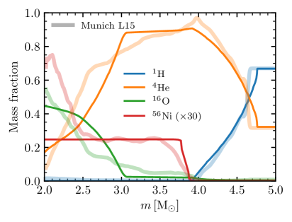
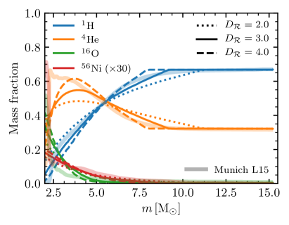
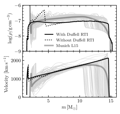
We now compare the 3D shell averages of Wongwathanarat et al. (2015) to MESA with Duffell RTI enabled. The left panel of Figure 27 shows the resulting abundances when the shock is at , with the thin lines from MESA with and the thick lines the 3D averages from the Munich L15 model. For H, He, and O, the MESA lines agree with the Munich model. If nothing is done to take into account the initial asymmetry of the explosion, the radial extent of the 56Ni in the Munich model far exceeds what can be achieved in MESA by Duffell RTI mixing. Hence, at this moment in the model evolution, we use the Munich L15 results to fix the extent of the MESA distribution of 56Ni. Later mixing in the MESA run is done by Duffell RTI. The right panel of Figure 27 shows the comparison with the Munich model just before shock breakout. For this case, we show three simulations with and 4.
In Figure 28 we show the MESA profiles of density (upper panel) and velocity (lower panel) at the moment when the shock is at . The solid lines are with Duffell RTI enabled, while the dotted lines are with it turned off. As shown by Wongwathanarat et al. (2015), Utrobin et al. (2017), and P. Duffell et al. (2017, in preparation) the operation of the RTI removes the unphysical density feature produced in 1D simulations without it. Such features can be seen in Figures 2 of Eastman et al. (1994) and Dessart & Hillier (2011) and in the dotted black line in the upper panel of Figure 28. Duffell RTI also alters the velocity structure of the material near the H/He boundary, as we discuss more in Section 6.6. The thick gray lines in both plots show the 1D shell averages of the 3D Munich L15 model. The fainter gray lines show the density and velocity profiles for a variety of angles in the Munich model. The asymmetries of the shock in the Munich model lead to its location varying between mass coordinates and . This variation with angle leads to 1D shell averages that do not show a sharp shock feature, but instead have more rounded shapes. Since the 1D MESA results have the shock at a single mass coordinate, they are similar to Munich profiles at a particular angle. This difference must be considered when comparing results from MESA to shell averages from the Munich model. It also shows that the time of shock breakout, which is well-defined in the 1D model, varies with angle in the 3D model.
6 Light Curves and Velocity Evolution of Core Collapse Supernovae
We now present MESA modeling of the ejecta evolution triggered by core collapse in massive stars (roughly ). The new MESA capabilities enable self-consistent calculations of photometric evolution of core collapse supernovae (SNe) using the STELLA code (Blinnikov et al., 1998; Blinnikov & Sorokina, 2004; Baklanov et al., 2005; Blinnikov et al., 2006). A public version of STELLA is now included with the MESA distribution, and the interface from MESA to STELLA has been customized for ease of use.555When using these capabilities one should cite this instrument paper and the following papers describing STELLA (Blinnikov & Sorokina, 2004; Baklanov et al., 2005; Blinnikov et al., 2006).
Our main emphasis in this section is on the commonly observed Type IIP “plateau” SNe that originate from energy deposited deep in the core of a red supergiant (Smartt, 2009b). We also exhibit how these new capabilities enable simulations of core collapse events that occur after the star has lost the majority of its outer hydrogen envelope, the Type IIb and Ib SNe.
The new capabilities we present are provided by a powerful combination of MESA and STELLA. Post core collapse evolution proceeds in two distinct phases. First we use MESA to evolve models from a few seconds after the central explosion triggered by core collapse to a time just before the outgoing shock reaches the stellar surface. These calculations make use of HLLC (Section 4) and Duffell RTI (Section 5). Subsequently, we use STELLA to evolve models through shock breakout and beyond the end of the plateau, generating light curves and velocities of the material at the photosphere and above.
Simulations using 3D models from the core collapse event to shock breakout are computationally expensive but now feasible (Wongwathanarat et al., 2015; Utrobin et al., 2017), and it will be a significant contribution to have more of them available in the future. To explore the subsequent 100 days of photometric and spectroscopic evolution, 1D approximations are common. The new capabilities with MESA and STELLA also use a 1D approximation for both the pre- and post-breakout evolution. This provides a less computationally costly alternative for initial exploration of the parameter space for potential progenitors prior to or instead of doing a more realistic but more computationally costly 3D simulation. The pair MESA and STELLA can produce useful results in a few hours running on a modern multicore desktop workstation (see Section 6.7), while the 3D pre-breakout evolution and post-breakout spectral analysis can take weeks running on a supercomputer. MESA and STELLA are not a replacement for the more computationally expensive codes but will be useful in conjunction with them.
Throughout this section, we present models that we characterize as “similar to” observed SNe. We list the properties and parameters of these models in Table 3. As we discuss in Section 6.8, where we describe the procedure by which these models were generated, they are not “best-fit” models. Rather, they simply serve as illustrative cases of these new capabilities.
6.1 From Core Collapse to Near Breakout with MESA
Models of massive stars can be evolved in MESA up to the onset of the rapid infall of the iron core (see Paper I, Paper II, Paper III). However, MESA cannot model the core collapse event itself. Hence, to transition from the onset of core infall to the explosion phase, we rely on a a variety of approximate procedures (Paper III).
For the current efforts, our approach is as follows. We remove the center section of the model at the location where the entropy per baryon is 4 , excising the portion of the model that will have collapsed to form a proto-neutron star. This corresponds approximately to the iron core, typically at about . We allow the model to continue infall until its inner boundary (IB) reaches km, near the location of the stalled shock (thanks to H.-T. Janka, private communication, for suggesting this scheme). After the first few seconds, we account for further fallback by removing negative velocity material at the IB. We are not seeking a numerical model of realistic fallback since that depends on 3D details of the explosion that are beyond what MESA can simulate.
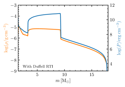
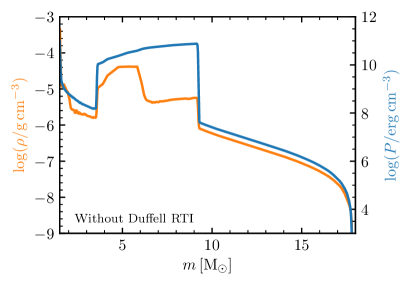
The stellar explosion is induced by injecting energy in a thin layer of approximately at the IB for 5 ms, at a rate sufficient to raise the total energy of the model to a user-specified value. In the subsequent evolution, nuclear reactions are allowed to change abundances but not to generate energy. This choice is suitable because we are not seeking accurate nucleosynthetic yields. The explosion energy spent to photodisintegrate the core to a mix of protons, neutrons, and alpha particles is soon after roughly repaid by energy released as those particles recombine to form products such as 56Ni. Getting an accurate accounting of the energy balance of that complex process is beyond the scope of this paper and is not attempted in the following examples. Our choice to exclude nuclear energy generation can be seen as a simplifying assumption that the cost of photodisintegration is balanced by the return from later recombination. For users wishing to refine this, any excess change in energy from nuclear reactions can be included in the specification of the post-explosion total energy of the model.
The conservation of total energy throughout the run is estimated by summing the per-step errors from post-explosion to near breakout. At each timestep, we compare the actual change in total energy between initial and final models for the step, to the change expected from surface luminosity and neutrino losses over the duration of the step. The runs for the models reported below typically show relative cumulative errors in conservation of total energy of less than 1%, with most of that error happening in the first few minutes post explosion when the shock is most extreme. For later stages, the cumulative relative error is orders of magnitude smaller.
The post-explosion evolution of the MESA model is determined by the shock traversal through the star and the resulting Duffell RTI. Figure 29 illustrates the difference between models with and without the effects of the RTI by showing density and pressure profiles. They are shown when the forward shock is about halfway through the star and when the reverse shock originating at the H/He boundary has reached on its way to the center. The reverse shock is primarily responsible for the large RTI effects evident in the plots. The online animated figure shows the time evolution of these and many other quantities of interest from seconds after explosion to near shock breakout.
6.2 From Near Breakout through the Plateau: Introducing STELLA
To follow the evolution of the model through shock breakout and beyond we use a multigroup (i.e., frequency-dependent) radiation hydrodynamics code.666MESA can be run through shock breakout and beyond, but we do not view gray opacity lightcurves as sufficient for quantitative comparisons to observed SNe. When the shock is near breakout, we hand the MESA model off to STELLA in an appropriate form which involves interpolating to the desired grid and optionally adding circumstellar material (CSM) according to user specifications. With that done, MESA is finished, and STELLA takes over (see Section 6.3 for a discussion of how we select when to hand off).
STELLA (Blinnikov et al., 1998; Blinnikov & Sorokina, 2004; Baklanov et al., 2005; Blinnikov et al., 2006) is able to model SN evolution at early times, before the expansion is homologous. It can also handle shock breakout and interaction with circumstellar material outside the conventional stellar photosphere. STELLA is an implicitly differenced hydrodynamics code that incorporates multigroup radiative transfer. The time-dependent equations are solved implicitly for the angular moments of intensity averaged over fixed frequency bands. STELLA takes about the same amount of time for near-breakout to post-plateau evolution as MESA takes to simulate from explosion to near-breakout: about an hour on current workstations.
STELLA solves the radiative transfer equations in the intensity momentum approximation in each frequency bin. We use from 40 to 200 frequency groups, enough to produce bolometric luminosities and broad-band colors, but not sufficient to produce spectra. Better broad-band light curves can be produced with the larger number of frequency groups, but 40 is sufficient for a bolometric lightcurve and gives faster runtimes since each group must be represented by a variable and an equation at each zone. The opacity is computed based on over 153,000 spectral lines from Kurucz & Bell (1995) and Verner et al. (1996). The expansion opacity formalism from Eastman & Pinto (1993) is used for line opacities taking high velocity gradients into account. The opacity also includes photoionization, free-free absorption, and electron scattering. LTE is assumed in the plasma, which allows the use of the Boltzmann-Saha distribution for ionization and level populations. STELLA does not include a nuclear reaction network except for the radioactive decay chain initiated from 56Ni. For calculating the overall opacity, the code uses 16 species: H, He, C, N, O, Ne, Na, Mg, Al, Si, S, Ar, Ca, a sum of stable Fe and radioactive 56Co, and stable Ni and radioactive 56Ni. Energy from nickel and cobalt radioactive decay is deposited as positrons and gamma-rays and is treated in a one-group transport approximation according to Swartz et al. (1995).
STELLA solves the conservation equations for mass, momentum, and total energy on a Lagrangian comoving grid. It employs artificial viscosity based on the standard von Neumann artificial viscous pressure used for stabilizing solutions (Von Neumann & Richtmyer, 1950) and a cold artificial viscosity used to smear shocks (Blinnikov et al., 1998; Moriya et al., 2013). The coupled equations of radiation hydrodynamics are solved through an implicit high-order predictor-corrector procedure based on the methods of Gear (1971) and Brayton et al. (1972); see Blinnikov & Panov (1996) and Stabrowski (1997) for details.
We explore the sensitivity of bolometric light curves () reported by STELLA to the number of frequency bins, spatial zoning, and error tolerances. The result of our sensitivity study is that 40 frequency bins, 300 spatial zones, and an error tolerance for the Gear-Brayton method typically give a converged model. In our experience using MESA and STELLA for Type IIP SNe, we have not found cases that require different values for number of frequency bins and error tolerance. Some cases may need a larger number of zones in order to minimize numerical artifacts producing spurious oscillations in the light curve. This problem can often be fixed by a relatively small increase in the number of zones; this is shown for a case similar to SN 2012A in Figure 30.
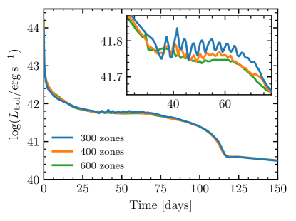
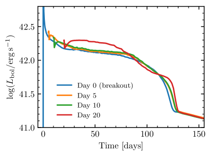
6.3 Handing Off from MESA to STELLA
A time must be chosen to hand off the MESA model to STELLA. This choice is driven by a compromise between two considerations. First, RTI modeling ceases once STELLA is running even though the effects of RTI may not be complete at that time. Therefore, one wants the model to remain in MESA as long as possible. But second, STELLA more accurately handles shock breakout and the outermost layers, especially if any matter is placed above the photosphere or if significant radiation is free-streaming from just below the photosphere prior to shock breakout. Moreover, the sophisticated multigroup radiation transfer of STELLA will do a much better job than (gray) MESA can at later times post breakout. Hence for longer-term lightcurve evolution, this motivates the default choice to perform this handoff just before breakout.
In order to illustrate the effects of this choice, Figure 31 shows bolometric light curves for cases where the handoffs are done at different times. Note that this plot shows MESA being forced to run post-breakout even though that is not recommended. The deviation of the light curves for later handoff are primarily the result of STELLA doing a better job because of its multigroup radiation transfer rather than any late-stage RTI effects being captured by MESA that are missed by STELLA. That is because, for this case, the H envelope is of normal thickness and the reverse shock from the H/He boundary has time to reach the center, completing essentially all of the RTI effects before breakout.
In the runs presented in the remainder of this section, we choose to do the MESA-to-STELLA handoff shortly before breakout, as determined by the outgoing shock front reaching a location below the surface of the model (this location is a user-defined parameter). Again, we note that in some cases the reverse shock is still far from the center at this moment, and not all of the RTI mixing has completed. In particular, this is true for models with a partially stripped envelope (see Section 6.9). For now, this remains a caveat for the user; a solution would be to have the post-breakout radiation hydrodynamics code include a treatment of the effects of RTI.
Because of STELLA’s treatment of radiation hydrodynamics, we have not had to take the progress of the model toward homologous expansion into consideration in selecting a time to hand off from MESA. However this is a consideration for doing a handoff to radiative transfer codes that assume homology. More accurate spectral and lightcurve modeling with full radiative transfer, such as EDDINGTON (Eastman & Pinto, 1993), SEDONA (Kasen et al., 2006), and CMFGEN (Dessart & Hillier, 2010), assume homologous expansion in their current applications to SNe, and this should be considered when deciding the time to hand off from another simulation. Indeed, Eastman et al. (1994) and Dessart & Hillier (2011) discuss this challenge, especially for the inner-most material that has not reached a homologous stage and can still have a reverse shock running through it. Approximations made in mapping to a thereafter homologous code can impact the late-time photospheric velocity evolution and the nebular line width predictions associated with the innermost ejecta.
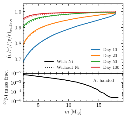
In contrast, STELLA does not assume homologous expansion, so early handoffs are fine; it can handle the effects of remaining pressure gradients as the model moves toward homologous expansion. This is important, as the time it takes to reach homology in these models can be quite long. Figure 32 shows velocity evolution results for a model similar to SN 1999em (see discussion in Section 6.8). Homologous expansion would imply that is flat, whereas a 20% variation from simple homology is evident at 20 days. An additional way in which homology can be violated long after shock breakout is from 56Ni decay, especially in Type Ia SNe (Woosley et al., 2007b). As is evident in Figure 32, the much smaller mass fractions of 56Ni in Type IIP SNe do not cause such a problem. The contrasting light curves with and without 56Ni are shown in Figure 33, exhibiting the prolonging of the plateau due to radioactive decay (Kasen & Woosley, 2009; Sukhbold et al., 2016a).
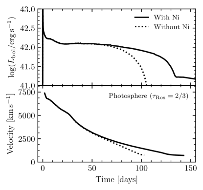
6.4 Connecting to Observations: Photospheric Properties from STELLA
To set the stage for the rest of this section, we describe a particular model in detail. Figure 34 shows the evolution of a model we construct to be similar to the Type IIP SN 1999em (99em_19 in Table 3). The quantities shown are those generated during the STELLA phase of the evolution. Panel (a) is the bolometric luminosity, while panel (b) shows velocity at the location of the photosphere (where ) and panels (c) and (d) show the mass and radius coordinate of this location. This illustrates the familiar result that the photosphere only reaches the deeper parts of the ejecta after about day 50. The radiation and gas temperatures at the photosphere are shown in panel (e), as is an effective temperature defined by the bolometric luminosity leaving the photosphere. Panel (f) shows the optical depth to the IB, highlighting that the radiative diffusion approximation is excellent (since ) until day 120, at which point the plateau ends and the IB temperature (panel g) approaches that of the photosphere. Meanwhile, the photospheric radius (panel d) stays remarkably constant throughout the plateau.
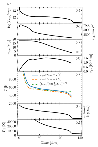
Our emphasis is on bolometric luminosities, where 40 STELLA frequency bins is adequate. However, broadband light curves are also reported by STELLA. Figure 35 shows how the STELLA colors change as one goes from 40 to 200 frequency bins in a model approximately matching the bolometric luminosity of SN 1999em (99em_19 in Table 3). This reflects that a given band is spanned by only a small number of frequency bins. The non-public research version of STELLA can opt to use many more frequency bins to address under-resolution issues. There are no current plans to include that capability in MESA. We also show what a blackbody would predict using the MESA colors module (see Appendix A). This makes it clear that the line-blanketing in the band is well handled by STELLA. We do not include colors in our subsequent discussions, but we expect they may be useful to users who have access to observations in one or two bands, but not enough data to produce a bolometric light curve from observations.
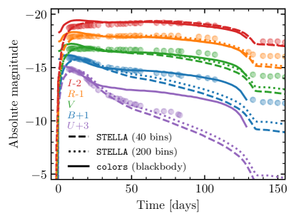
6.5 Connecting to Observations: Fe II Line Velocities
It is important to be able to interpret the ejecta velocities measured by observers, which are often inferred from the absorption minimum in the Fe II 5169 Å line. Modeling these absorption features requires more detailed radiative transfer than available in STELLA. However, rather than assume the photospheric velocity reported by STELLA is identical to the Fe II 5169 Å line, we have added the capability of finding the location (and hence the velocity) of material above the photosphere where the Sobolev optical depth in the Fe II 5169 Å line is a specified value.777This approach arose through the efforts of Dan Kasen, who also provided important data needed to complete the calculation. This will prove to be most important after day 30 or so, when the photosphere has started to move inward in mass coordinate into ejecta with a shallow density profile.
The strength of a line in a homologously expanding atmosphere is quantified by the Sobolev optical depth (Sobolev, 1960; Castor, 1970; Mihalas, 1978; Kasen et al., 2006), which for the Fe II line at any position is
| (53) |
where Å is the line center wavelength for the Fe II line, is its oscillator strength, is the number density of iron atoms, and is the time since breakout. The quantity is the fraction of iron atoms that are in the lower level of the transition of interest and depends on the properties of the gas. D. Kasen (2017, private communication) provided an table for post-processing to produce the Fe II line velocities, calculated under the assumption of LTE and covering to and to .
We use Equation (53) after the STELLA run to provide the velocity of material that satisfies a chosen value of . This yields a velocity that can be compared to the measured Fe II line velocities. Figure 36 shows the resulting comparisons for various choices of for a model similar to the Type IIP SN 2012A found solely by matching the bolometric luminosity (upper panel). The lower panel displays the Fe II 5169 Å data and the velocities derived from the photosphere and for a range of values of . At early times, there is little difference between the photospheric velocity and that of the Fe line. However, as the photosphere moves deeper into the ejecta, the two velocities substantially diverge. The velocity inferred from the Sobolev argument gives a much better match to observations than the photospheric velocity. Motivated by this comparison, we choose for our later plots, a parameter that the user is free to adjust.
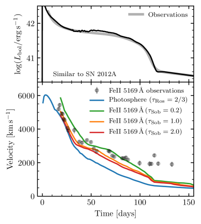
6.6 The Impact of Pre-breakout RTI Mixing
We have previously outlined the inclusion of a method for RTI mixing in MESA (the Duffell scheme; Section 5), the use of MESA to evolve models pre-breakout (Section 6.1), the use of STELLA to evolve models post-breakout (Section 6.2) and described how to connect the models to observations (Sections 6.4 and 6.5).
In this way, MESA plus STELLA allows users to explore the impact of RTI mixing on Type IIP light curves and velocities. Prior work in this direction (Eastman et al., 1994; Utrobin, 2007; Dessart & Hillier, 2010, 2011; Morozova et al., 2015) focused on the impact of compositional mixing, often with averaging approaches to achieve various levels of mixing. Only the recent work of Utrobin et al. (2017) incorporated compositional mixing from a 3D model and also included the modified density and velocity structures, also seen in the 1D RTI mixing (P. Duffell et al. 2017, in preparation).
Figure 37 shows the lightcurve and velocities of model 99em_19. The luminosity without RTI mixing has a distinctive rise just before the plateau as shown by Eastman et al. (1994) and Utrobin (2007). As RTI causes many associated changes in composition, density, velocity, and energy density for the innermost material, we cannot specifically identify the immediate cause of the lengthening of the plateau phase when RTI is incorporated without further experiments. These are now possible using MESA and STELLA but are beyond the scope of this paper. The lower panel shows the photospheric and Fe II line velocities with and without RTI mixing. The most evident change is at the end of the plateau, when the material that was near the H/He boundary in the red supergiant is approaching the SN photosphere. That material is strongly affected by RTI mixing as shown in Figure 28 and discussed in P. Duffell et al. (2017, in preparation).
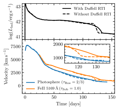
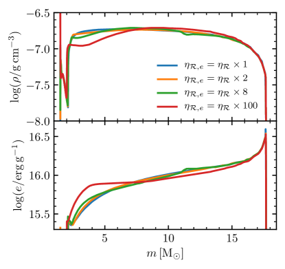
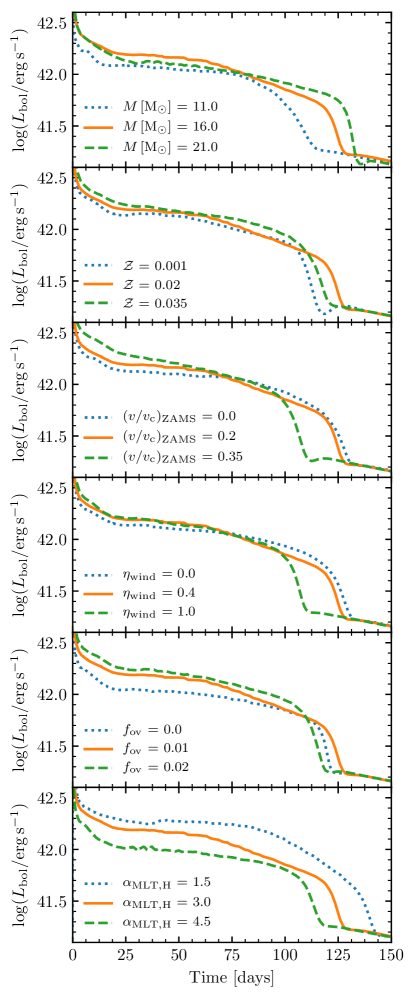
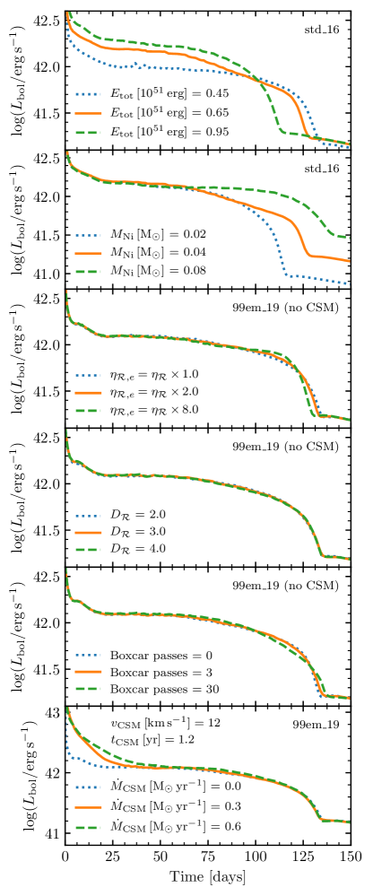
To enable exploration of the impact of various components of the RTI mixing, we explicitly allow for the diffusion coefficients for density, momentum, energy, and composition to be scaled by independent constant factors relative to the value given in Equation (47). We show in Figure 38 the impact of varying the coefficient in the internal energy flux in Equation (48), which we refer to as . These plots show the energy density and density of the ejecta just before shock breakout in one of our models (99em_19) in Table 3). The blue line is for the fiducial value, whereas the red line is for an extreme increase of a factor of 100. The only locations that are sensitive to these changes are the innermost mass coordinates where RTI was most active, the same regions where the lightcurve and velocities seem to be sensitive to changes related to RTI mixing. The variable was found to be a useful “knob” to vary for modeling of specific SNe.
6.7 Exploring the Explosive Landscape
A strength of the new MESA plus STELLA capabilities is their ease of use. This enables detailed quantitative studies of large numbers of core collapse SNe. The open source nature of MESA, the inclusion of STELLA in the MESA distribution, and the repository of examples contained within the MESAstar test suite allow a user to obtain models that can be compared directly to observations. Indeed, with minimal manual intervention, a user can take a star from the pre-MS to a SN light curve within a few hours of computer runtime. To emphasize this point, we describe here how this might be done (Section 6.7.1). To demonstrate how parameter choices affect lightcurves, we show a large sample of variations of a standard case for “high-middle-low” settings of some of the main parameters (Section 6.7.2). In Section 6.8 we will exhibit a few specific models created to be roughly similar to known Type IIP SNe. The potential is clear for an extensive database of such SNe models created using MESA and STELLA; its actualization is beyond the scope of this paper.
6.7.1 Generating Models with MESA plus STELLA
The first step in generating a core collapse SN lightcurve is to use MESA to make a pre-SN stellar model that is undergoing core collapse. The test case example_make_pre_ccsn can serve as a useful template. As part of the required inlists, the user must select values for the main variables: initial mass (), initial metallicity (), initial rotation (), overshooting parameter (), wind scaling factor (), and the mixing length for MLT in the H envelope ). Of course, the user may tune other MESA parameters of interest. The run from pre-MS to Fe core infall runs automatically given these parameters and, depending on the case, takes roughly an hour on a modern multicore desktop workstation. Users interested in details of pre-SN models may require settings that lead to significant additional runtime (e.g., Farmer et al., 2016; Renzo et al., 2017).
The second step loads the model at core infall into MESA, emulates the core collapse explosion by excising the core and injecting energy and Ni (as described in Section 6.1) and evolves until near shock breakout. The test case example_ccsn_IIp can serve as a useful template. Again, the user must set the value of the various “knobs” controlling the properties of the explosion such as the total energy and the 56Ni mass . Early ( days) lightcurves of core collapse SNe are better fit when large amounts of CSM are placed outside the conventional photosphere (Morozova et al., 2016; Dessart et al., 2017; Morozova et al., 2017a, b). We provide an option to include CSM. We also provide the option for “boxcar” smoothing of the model abundances before the handoff from MESA to STELLA (Kasen & Woosley, 2009; Dessart et al., 2013; Morozova et al., 2015). The end result of this step is a model suitable for input into STELLA, so one must also indicate the number of STELLA zones to be used. This MESA phase from after explosion to near breakout typically takes about 30 minutes on a modern multicore desktop workstation.
The final step uses the results produced in the previous step as input to STELLA and evolves the model through shock break-out to the post-plateau phase. A script to execute STELLA is provided. This stage takes about an additional 30 minutes on a modern multicore desktop workstation for typical cases. When STELLA finishes, a post-processing step produces data for comparison to observational results.
6.7.2 Sensitivity to Variations in Key Parameters
Figure 39 exhibits the std_16 model lightcurves as progenitor parameters are varied. Many variations behave as expected from previous analytical and numerical scalings (Popov, 1993; Kasen & Woosley, 2009; Sukhbold et al., 2016a). For example, the decrease in the plateau duration with lower ZAMS masses or higher mass loss (increased ) is as expected. The increase in plateau luminosity with decreasing is because those stars with lower have a larger stellar radius at time of explosion. However, other variations in these figures are not as easily diagnosed.
Figure 40 exhibits model lightcurves as explosion parameters are varied. Again, many cases lead to the expected outcomes, such as the increase in the plateau luminosity with increasing explosion energy and the increased duration of the plateau with increasing nickel mass. The changes caused by varying the RTI parameters are slight for the compositional mixing and boxcars, though, as we discussed in Section 6.6, modifying the diffusion of energy density during RTI does impact the shape at the end of the plateau. The impact of the CSM is similar to that shown by Morozova et al. (2017a) and Dessart et al. (2017).
With experience in the effects of varying the parameters (knobs) shown in Figures 39 and 40, it is sometimes possible to get a rough match between model and observations after a dozen or so attempts. That is about the amount of effort we undertook to get the models similar to various observed SNe presented in Section 6.8. Of course the effects of the various knobs do not combine in any simple manner, so it can be a nontrivial challenge to find a combination that gives a good match for both velocities and lightcurve. Our experience suggests that it is a good strategy to match velocities before lightcurves since there are few ways available to shift velocities and many ways to change lightcurves. It is important to include velocities in judging potential matches because of the multiple degeneracies, as will be seen below where we show two models similar to SN 1999em with quite different ejecta masses and explosion energies. Even when using both velocities and lightcurves, it remains a challenge to find a unique “best” match.
| progenitor parameters | stellar properties at time of explosion | explosion parameters and properties | |||||||||||||||||||||
|---|---|---|---|---|---|---|---|---|---|---|---|---|---|---|---|---|---|---|---|---|---|---|---|
| case | case | case | boxcar | ||||||||||||||||||||
| std_16 | 16.0 | 0.02 | 0.2 | 0.4 | 0.01 | 3.0 | 14.5 | 3960 | 759 | 5.11 | 5.58 | 1.58 | std_16 | 1.58 | 12.9 | 0.04 | 1.0 | 0 | 0.0 | 0.0 | 0.0 | ||
| 99em_16 | 16.0 | 0.02 | 0.2 | 0.4 | 0.01 | 3.0 | 14.5 | 3960 | 759 | 5.11 | 5.58 | 1.58 | 99em_16 | 1.58 | 12.9 | 0.042 | 2.0 | 3 | 1.0 | 0.25 | 10 | ||
| 99em_19 | 19.0 | 0.02 | 0.2 | 0.4 | 0.00 | 3.0 | 17.8 | 4490 | 603 | 5.13 | 6.58 | 1.50 | 99em_19 | 1.50 | 16.3 | 0.042 | 1.0 | 3 | 1.2 | 0.30 | 12 | ||
| 05cs | 13.0 | 0.006 | 0.0 | 0.1 | 0.01 | 3.0 | 12.9 | 4280 | 537 | 4.95 | 4.37 | 1.57 | 05cs | 2.51 | 10.4 | 0.009 | 7.0 | 1 | 1.0 | 0.30 | 10 | ||
| 09N | 13.0 | 0.006 | 0.0 | 1.0 | 0.01 | 3.0 | 11.6 | 4290 | 549 | 4.96 | 4.34 | 1.67 | 09N | 1.67 | 9.9 | 0.028 | 30.0 | 3 | 1.4 | 0.30 | 10 | ||
| 12A | 11.8 | 0.02 | 0.2 | 0.1 | 0.002 | 3.0 | 11.6 | 4300 | 525 | 4.94 | 4.08 | 1.49 | 12A | 1.49 | 10.1 | 0.009 | 3.0 | 2 | 0.9 | 0.30 | 10 | ||
| 13bvn | 11.0 | 0.02 | 0.0 | 0.0 | 0.01 | 2.0 | 3.4 | 26520 | 7.24 | 4.37 | 3.40 | 1.57 | 13bvn | 1.57 | 1.8 | 0.110 | 1.0 | 5 | 0.0 | 0.0 | 0 | ||
| stripped | 17.0 | 0.02 | 0.3 | 0.0 | 0.01 | 3.0 | — | — | — | — | — | — | stripped | — | — | 0.037 | 1.0 | 20 | 0.0 | 0.0 | 0 | ||
6.8 Applications to a Few Type IIP SNe
To show examples of what can be accomplished with these new capabilities, we have modeled four Type IIP SNe: 1999em, 2005cs, 2009N and 2012A. These cover a range of luminosities, plateau durations and nickel masses and have readily available data (Pejcha & Prieto, 2015a, b) for bolometric luminosities and Fe II velocities.888We especially thank Ondřej Pejcha and Stefano Valenti for providing the necessary data. We follow the steps described in Section 6.7, iterating to reach the matches shown. The models are not intended to demonstrate the best matches that can be achieved using MESA and STELLA. An investment of more effort could produce better matches, but is beyond the scope of this paper. The parameters we choose are shown in Table 3.
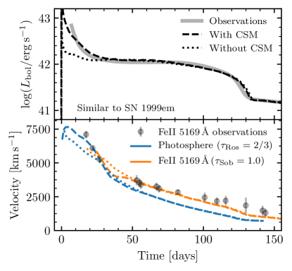
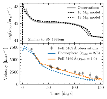
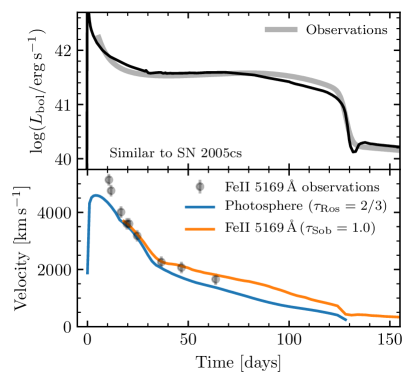
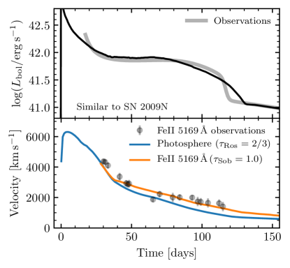
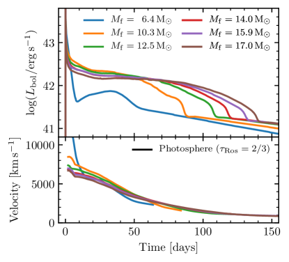
We note a few general insights gained from our modeling. We found that the radii of red supergiant models from MESA were too large for these Type IIP SNe models unless we set . All models benefited at early times by having some CSM present. Figure 41 shows how the early 1999em model predictions change as CSM is added to the value shown in Table 3. The luminosity at early times is a far better match, as are the earliest velocity data. As expected, by day 50 and beyond there is no impact of the CSM on the model predictions. Comparisons of how the luminosity collapsed at the end of the plateau drove us to prefer an enhancement in in several cases.
To exhibit some of the possible degeneracies, we constructed two distinct models for 1999em. As shown in Figure 42, they are both reasonable models for the bolometric luminosity and Fe II velocities. However, their ejected masses and radii differ significantly, one has and , whereas the other has and . Utrobin (2007) gave an ejected mass of , a radius of , and an explosion energy of erg. Bersten et al. (2011) gave an ejecta mass of , radius of , and explosion energy of erg. Utrobin et al. (2017) model this event with a 3D simulation from explosion to shock breakout, similar to the Munich L15 model we discuss in Section 5, but with an explosion energy of about erg. For comparison, the MESA models for 1999em have total energies after explosion of erg for the case with ejected mass, and erg for the case with ejected mass.
We previously showed 2012A in Figure 36. Our model had an ejected mass of to compare with from Morozova et al. (2017b), from Tomasella et al. (2013) and from Utrobin & Chugai (2015). Tomasella et al. (2013) also reported a progenitor luminosity of , just a bit fainter than our model’s value. Figure 43 shows our model for 2005cs. Our model has an ejected mass of , slightly higher than the reported by Spiro et al. (2014) and the reported by Morozova et al. (2017b). Figure 44 shows our model for 2009N, which has an ejected mass of , whereas Morozova et al. (2017b) found and Takáts et al. (2014) found .
6.9 Partially Stripped Core Collapse SNe
There is a well-defined class of core collapse SNe where either much (Type IIb) or nearly all (Type Ib and Ic) of the H envelope was lost prior to the core collapse event. Dessart et al. (2015) performed detailed radiative transfer models for a large set of progenitors from binary evolution, while Morozova et al. (2015) carried out diffusive calculations with varying amounts of mass loss. Yoon et al. (2017) explored MESA models constructed from binary transfer scenarios and applied them to a set of well observed Type IIb events. We have not yet been able to deal successfully with Ic models because of numerical problems related to the extreme ejecta velocities that occur at shock breakout. However, it is possible to do both IIb and Ib models as shown here.
In Figure 45, we show the MESA plus STELLA predictions for luminosities and photospheric velocities for a range of models with varying amounts of mass stripped from a ZAMS model, ranging from the entire initial H envelope still remaining down to only of the H envelope left at the time of explosion. Similar to Figure 7 of Morozova et al. (2015), the plateau period becomes shorter as the residual H shell mass declines. Our smallest mass model has an H envelope mass comparable to typical models of Type IIb SNe and generates a light curve comparable to observed Type IIb SNe (Ergon et al., 2015). Figure 46 shows the interior properties of these same models near the moment of shock breakout. For models which have been stripped, the reverse shock has not reached the IB at the time the forward shock reaches the surface. Since RTI mixing does not occur in STELLA, these models would incompletely include the effects of the RTI.
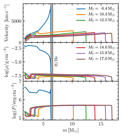
Cao et al. (2013) discovered the fully stripped Type Ib SNe iPTF13bvn in the nearby spiral galaxy NGC 5806 with the intermediate Palomar Transient Factory (Law et al., 2009). This is one of only a few stripped SNe with a progenitor detection. Using data from Cao et al. (2013) and Fremling et al. (2014), we show in Figure 47 our model that approximately matches the iPTF13bvn light curve. The model is derived from an ZAMS model and has a remaining mass of only at the time of explosion with total energy after explosion of ergs and a 56Ni mass of distributed throughout the remaining star (ejecta mass 1.8 ). Fremling et al. (2014) also modeled this lightcurve, finding the total energy to be ergs, with a a 56Ni mass of , and total ejecta mass of . Our parameters are similar, falling within the range of the quoted uncertainties, except for the 56Ni mass.
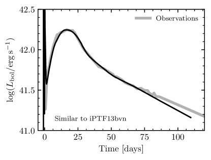
7 Black Hole Formation
Compact objects are a natural product of the evolution of massive stars. A broad consensus on which massive stars produce black holes (BH) has not yet been reached (Timmes et al., 1996; Fryer & Kalogera, 2001; Heger et al., 2003; Eldridge & Tout, 2004; Zhang et al., 2008; Ugliano et al., 2012; Clausen et al., 2015; Sukhbold et al., 2016b; Müller et al., 2016; Limongi, 2017).
The lack of consensus is due to a variety of differences in the modeling, including stellar wind treatments during the pre-supernova stage (Renzo et al., 2017); shellular rotation prescriptions (e.g., Limongi, 2017); sensitivity to the initial metallicity (e.g., O’Connor & Ott, 2011), number of isotopes in the reaction network (Farmer et al., 2016), adopted values of critical reaction rates (deBoer et al., 2017; Fields et al., 2017), and ignition of core carbon burning (Farmer et al., 2015; Cristini et al., 2017; Petermann et al., 2017); variations from spatial and temporal resolution (Farmer et al., 2016); convection during core-collapse (e.g., Couch et al., 2015); and effects from binary partners (e.g., Marchant et al., 2016; Batta et al., 2017). In addition, current estimates of the neutron star and BH initial mass function chiefly rely on parameterized explosion models and not on first principles calculations.
This section explores MESA models that can produce BHs. First, we consider 60 models that can form a BH without encountering dynamical instability due to pair production. Second, we survey 60 models that encounter dynamical instability, either entering the 4/3 regime once to produce a pair-instability supernova (PISN) (Fowler & Hoyle, 1964; Rakavy et al., 1967; Rakavy & Shaviv, 1967; Barkat et al., 1967; Fraley, 1968; Ober et al., 1983; Fryer et al., 2001; Scannapieco et al., 2005; Kasen et al., 2011; Chatzopoulos et al., 2013), or multiple times to produce a pulsational pair-instability supernova (PPISN) and a BH remnant (Barkat et al., 1967; Woosley et al., 2007a; Chatzopoulos & Wheeler, 2012; Woosley, 2017).
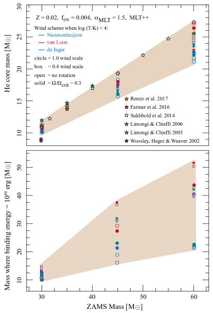
7.1 Progenitors that Do Not Pulse
The upper panel of Figure 48 shows the He core mass from =0.02 =30, 45, and 60 models. The lower panel shows the mass location where the binding energy is . Each ZAMS mass uses an exponential convective overshoot parameter =0.004 applied at all convective boundaries, a mixing length =1.5, MLT++ enabled (see Paper II), and is run to the onset of core-collapse (infall velocity 1000 km s-1). We illustrate the variation in the He core mass and mass location where the binding energy is from the effects of rotation, wind strength, and the wind schemes of Nieuwenhuijzen & de Jager (1990), van Loon et al. (2005), and de Jager et al. (1988).
To estimate a BH mass from the structure at core collapse, we use the mass location where the binding energy integrated from the surface exceeds 1048 erg. This is motivated by neutrinos removing 1053 erg during core-collapse, reducing the gravitational mass of the core by 0.3 . The outer part of the star responds to the sudden decrease in the gravitational field by driving a sound wave that steepens into a shock that unbinds some of the outer envelope (Coughlin et al., 2017). Mass with binding energy 1047 erg is likely to be ejected (Nadezhin, 1980; Lovegrove & Woosley, 2013) while mass that is not ejected will likely become part of the BH. Figure 48 suggests that BH masses estimated in this simple way can be significantly larger than the final He core mass, and more sensitive to the assumed model parameters. For example, there is wide variation in the expected BH mass for the 60 progenitor depending on choice of wind scheme and scaling factor, whereas modest rotation has a smaller effect.
7.2 Pulsational Pair-instability Supernovae
Stars with 60 are expected to become dynamically unstable before core O depletion as pair production leads to regions where the adiabatic index 4/3 (Fowler & Hoyle, 1964; Rakavy & Shaviv, 1967). The ensuing collapse results in explosive O burning, with a variety of possible outcomes. Stars can produce PISNe where the energy injected from explosive O burning completely unbinds the star without leaving a compact remnant. Alternatively, stars can undergo a cyclic pattern of entering the pair instability region, contracting, burning, and expanding, leading to PPISNe.
Individual pulses in a PPISN can remove a large fraction of the mass of the star at velocities of several thousand km s-1, with the remaining material settling down into hydrostatic equilibrium at a lower central temperature than before the pulse. The star then contracts as it loses energy due to radiation and neutrino emission until it undergoes an additional pulse or collapses to form a BH. Depending on its initial mass, the time between pulses varies from a fraction of a year to millennia, with the outer ejected layers expanding to very low densities and becoming optically thin.
MESA currently cannot simultaneously follow the long term evolution of the bound core and the ejecta, making it necessary to remove the unbound layers from the stellar model. To do this we model individual pulses using both the Riemann solver hydrodynamics (Section 4), as well as the 1D treatment of the Rayleigh-Taylor instability (Section 5), until the star is approximately in hydrostatic equilibrium. We then relax a new stellar model using the methods described in Appendix B, such that it has the same mass, entropy, and composition profiles as the layers that remained bound in the hydrodynamical model. This model is then evolved assuming hydrostatic equilibrium until the onset of another pulse or the final core-collapse to a BH.
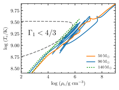
As an example, we compute models at a metallicity , using similar parameters as in Section 7.1. The van Loon scheme is used for low-temperature winds with a scaling factor of . In addition, convection is modeled as a time-dependent process by limiting changes in convective velocities as in Arnett (1969) and Wood (1974).
Figure 49 shows the evolution in the - plane during late burning stages for a model undergoing a PPISN, a model experiencing iron-core collapse, and a model producing a PISN. Although the center of the star does not evolve into the region where , the outer layers of the CO core do. Coupled with enhanced neutrino losses from pair-annihilation, this causes the star to collapse and undergo four distinct pulses before finally collapsing into a BH. At the onset of the first pulse, the star has a mass of , with a He core of and a CO core of . As shown in Figure 50 the first two pulses happen within two days of each other and they remove the entire H envelope. The remaining two pulses remove almost the entire He envelope, resulting in a final mass of when the star collapses into a BH.
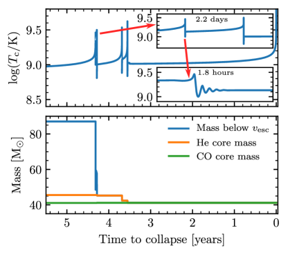
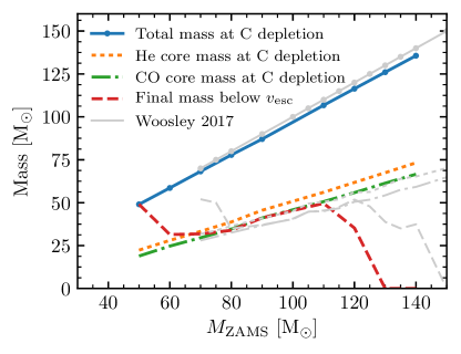
Figure 51 shows key masses on a grid encompassing ZAMS masses for which PPISNe occur under our model assumptions. Our PPISN progenitors have He core masses in the range of , and no BHs with masses above are formed. These results are in broad agreement with Woosley (2017).
8 Energy Accounting in Stellar Evolution
Paper I describes the stellar structure equations and their implementation in MESA. In order to provide physically and numerically accurate solutions of these equations, it is often necessary to evaluate them in different ways depending on the details of the star being simulated. In particular, there are a number of different ways to formulate and evaluate the equations solved by MESA that encode local and global energy conservation. The goal of this section is to clarify the available options, discuss when and why they are used, and describe how various forms of energy are tracked and accounted for in stellar evolution. While in places this section reads like a tutorial, it is in fact the first time we have presented a detailed description of a complex and critical aspect of how MESA works, information that is important for intelligent use of this software tool.
In Section 8.1 we describe the fundamental equations we are solving, and in Section 8.2 we describe choices associated with their numerical implementation. In Section 8.3 we describe the connection between the form of the energy equation typically used in stellar evolution calculations and the version used when the hydrodynamics options discussed in Section 4 are enabled. In Section 8.4 we clarify how the energy associated with ionization is included in MESA. In Section 8.5 we describe the numerical approach necessary to ensure that the latent heat associated with crystallization in a white dwarf (WD) is included in MESA. In Section 8.6 we discuss the difficulties introduced by the necessity to blend between different equations of state (EOS) as the thermodynamic conditions in the stellar interior change, and how MESA minimizes artifacts associated with these blends. In Section 8.7 we discuss the energy associated with gravitational settling.
8.1 Fundamental Equations
In the stellar structure equations (e.g., Cox & Giuli, 1968; Kippenhahn et al., 2012), energy conservation is typically formulated by considering the energy flow in and out of a fluid parcel. In this Lagrangian picture, to understand how the energy of a fluid parcel is changing, we account for the specific (i.e., per unit mass) rate of energy injection into the parcel, , and the specific rate of energy flow through the boundaries (; is the luminosity profile and the Lagrangian mass coordinate). The specific heating rate () for the parcel must then satisfy
| (54) |
where is the Lagrangian time derivative. Except in the case of hydrodynamics described in Section 4 (where a total energy equation is solved; see Section 8.3), the basic equation to be solved is always some form of Equation (54). By tradition, the negative of the left-hand side of Equation (54) is called .
Thermodynamics relates the heating of material to the changes in its properties. The first law of thermodynamics states that the total heat added for a parcel is
| (55) |
where is the internal energy, is the pressure, and is the volume. Let be the number of particles of species in the parcel. Then expanding in terms of the independent thermodynamic basis variables yields the following thermodynamic identity:
| (56) |
where is the entropy, and is the temperature. The sum runs over all species present, and
| (57) |
is the chemical potential for species .
The number abundance of every species is defined with reference to the total number of baryons as . Denoting Avogadro’s number by , the atomic mass unit is . The specific (i.e., per unit mass) form of Equation (56) is then given by multiplying by the invariant to find
| (58) |
The total baryonic mass density is , so that is the specific volume, and and are specific energy and entropy respectively. Local thermodynamic equilibrium (LTE) determines a unique solution for the ionization state of each isotope. Thus, composition is completely specified by a set of number abundances for all nuclear isotopes.
Equation (58) is relativistically correct when the rest mass is included in the energy and the chemical potentials. Therefore, in principle, changes in nuclear rest masses due to nuclear reactions could be accounted for via this equation. However, in MESA, the energetic effects associated with composition changes due to nuclear reactions are not included in . Instead, these important terms are accounted for via (the specific energy generation rate of nuclear reactions) which is evaluated separately and included as part of the local source term in Equation (54) (see Paper I).
It is often convenient to specify compositions in terms of the baryonic mass fractions via the relation , where is the mass number for isotope . Since rest-mass changes due to nuclear reactions are handled separately from , and can be treated as independent basis variables without introducing any ambiguity into the chemical potential term in Equation (58). Some EOS options express the composition dependence in terms of aggregate quantities; examples include hydrogen abundance , helium abundance , metallicity , average mass number , and average atomic number .
8.2 Implementation
Basic variables are those quantities directly calculated by MESAstar’s solver. Examples include velocity, radius, and the thermodynamic variables. MESA offers options for selecting or as the thermodynamic variables. The EOS routines calculate other thermodynamic quantities as a function of the chosen variables, e.g., . MESA solves the stellar structure equations implicitly, thus it is possible to approximate total time derivatives of any quantity calculated in the stellar model simply by differencing its value at the start and end of a timestep. Therefore, one way to evaluate would be to directly calculate the time derivatives in Equation (58). Two possible versions of would then be
| (59) |
and
| (60) |
While simple to construct, the finite differences necessary to calculate these equations are often numerically problematic.
To see the potential numerical issues, consider the implementation of Equation (54) using Equation (60) in cell with mass over a timestep . The derivative of a quantity is typically constructed as a finite difference of over the timestep, so after integrating over the mass of zone , we have
| (61) | ||||
The implicit solver scheme in MESA attempts to reduce the residual from evaluating the right hand side of this equation below some tolerance.
While the implicit scheme in MESA may sometimes find acceptable results for an equation such as Equation (61), finite numerical precision can result in troublesome behavior for the time derivatives involving subtractions. In particular, over a small timestep where the change in or is small compared to the overall magnitude of these quantities, floating point arithmetic can suffer significant loss of precision. When energy scales arising from these types of finite difference derivatives are comparable to , the implicit solver may be unable to converge to an acceptable solution.
To avoid these problems, the equations can be cast in terms of derivatives that are not evaluated using subtractions. Such derivatives are available only for the basic variables, since the Jacobian matrix for an evolution step satisfying the equations of stellar structure in MESA is written in terms of the basic variables and their derivatives (see Paper I, Section 6.2 and Paper II, Section B.2 and Figure 47). For MESA, and serve as default variables.
Modifying Equation (60) to take advantage of as a basic variable yields
| (62) |
but the change in is still evaluated using subtraction. Another related form, obtained by application of mass continuity, is
| (63) |
where is the cell velocity and is the area of the cell face. This is the form used in the artificial viscosity based hydrodynamics options described in Paper III.
Expanding the total derivative of energy and thus eliminating the subtraction motivates the following alternative forms. Expanding in terms of its dependence on the basic variables and and dropping the dependence on composition gives
| (64) |
where . One can also choose to expand in terms of its dependence on and (dropping composition dependence) and then convert to a form given in terms of instead of to obtain
| (65) |
where and . The derivation for this expression in terms of and is given in Chapter 4 of Kippenhahn et al. (2012), from which it is straightforward to obtain Equation (65) using and .
Since and are basic variables, the time derivatives appearing in Equations (64) or (65) involve no subtractions. Hence, solving Equation (54) with as defined by those two equations will not be susceptible to the same losses of numerical precision as other forms, at the cost of dropping the composition terms. Similarly, Equation (4.47) of Kippenhahn et al. (2012) will yield the same stability when and are used as basic variables. When and are selected as basic variables, the identification allows writing
| (66) | ||||
Section 4.5 in Kippenhahn et al. (2012) also shows how this local energy treatment of results in global energy conservation, including total gravitational potential energy from which the name is derived.
The superior numerical stability of Equations (64)–(66) comes at the cost of using derivative quantities such as and . The Jacobian matrix of an implicit method thus requires the partial derivatives of and . An EOS must therefore be capable of returning the state functions , , and along with their first derivatives (e.g., and ) and second derivatives (e.g., ).

| Inlist Option | |
|---|---|
use_PdVdt_form_for_eps_grav |
(60) |
use_dlnd_dt_form_for_eps_grav |
(62) |
use_dedt_form_of_energy_eqn |
(63) |
use_dEdRho_form_for_eps_grav |
(64) |
MESA default (all other inlist options .false.) |
(65) |
lnPgas_flag (and other inlist options .false.) |
(66) |
use_lnS_for_eps_grav |
(67) |
As noted above, Equations (64)–(66) drop the composition terms, which is justifiable if the derivatives are negligible for each . Dropping composition terms is often justified in stellar evolution scenarios where timescales for these changes are very slow or their associated energies are negligible, such as MS burning where energy release from nuclear burning dominates any small changes in internal energy due to composition evolution over a single step (Kippenhahn et al., 1965; García-Berro et al., 2008). Making this assumption, MESA also offers an option for calculating in terms of a simplified form of Equation (59):
| (67) |
which drops composition dependence to offer an expression that is more convenient to evaluate.
However, even after composition dependence related to nuclear burning is accounted for with a separate term as discussed in Section 8.1, other processes that change abundances (e.g., mixing) may be important. In cases where dropping these terms is not justifiable, it may be necessary to add a compensating local source term in Equation (54).
In summary, MESA currently offers options for solving Equation (54) with defined in any of the ways given in Equations (60)–(67). Figure 52 schematically summarizes the relationships between these equations and Table 4 shows the inlist commands necessary for invoking each of these options. Usually, the superior numerical stability gained by using Equation (65) is to be preferred, and hence it is the MESA default, but users should be aware of the possibility that other forms may be necessary to capture important physics. One such case for Equation (67) is described in Section 8.5. Another is the artificial viscosity-based implicit hydrodynamics described in Paper III (see Section 4, Equation 41), where choosing Equation (63) helps ensure intrinsic energy conservation.
8.3 Relationship to the Riemann Solver-Based Hydrodynamics Implementation
When using the Riemann solver-based hydrodynamics capabilities described in Section 4, MESA does not cast the stellar structure equations in terms of local heating as in Equation (54). Instead, it combines Equation (54) with the constraint of fluid momentum conservation to form a local total energy equation.
We begin with the mass continuity equation,
| (68) |
and the momentum equation,
| (69) |
written in Lagrangian form and assuming spherical symmetry. The variable is the radial velocity and is the gravitational potential. The Lagrangian derivative operator is .
Multiplying Equation (69) by gives
| (70) |
The gravitational potential does not explicitly depend on time (), so . This implies
| (71) |
Using Equations (54) and (60) we have
| (72) |
Adding Equations (71) and (72) gives
| (73) |
Using mass continuity (Equation 68) this becomes
| (74) |
In spherical coordinates
| (75) |
where . Thus we arrive at the equation that MESA solves,
| (76) |
8.4 Ionization
The internal energy reported the EOS should include the energy associated with ionization999Since this energy is released upon recombination, it is also often referred to as “recombination energy”. and molecular dissociation. The assumption of LTE specifies the ionization state given . Since MESA does not regard a change in ionization as a change in composition, it is not necessary to include separate composition derivatives in in order to account for the energetic effects of changes in ionization state.
To demonstrate a specific scenario where MESA accounts for ionization energy, we evolve a pre-MS model composed of pure H. We compare quantities calculated by MESA with other, simpler estimates. We calculate the thermal energy assuming a monatomic ideal gas,
| (77) |
We calculate the ionization energy for pure H as
| (78) |
where we assume the ionization fraction of H is given by the Saha equation. The variable represents the neutral fraction of H. The H ionization energy is and Equation (78) also includes the dissociation energy of molecular H () assuming that no H is in the molecular state.
During the evolution, we record calculated by MESA using Equation (65). We also evaluate the quantity
that separates out the thermal and ionization energy. In Figure 53 we compare these two approaches, making it clear that all three terms in the above expression play an important role. Their sum agrees with the MESA , indicating that each of these terms is accounted for in the MESA calculation.
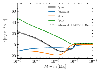
Figure 54 shows the history of the material at the Lagrangian coordinate . We plot reported by the MESA EOS along with and (calculated in same manner as above). At this location, the specific internal energy is dominated by the ionization energy. The lower panel of this figure shows the neutral fraction of H; towards the left of the plot, the H is fully neutral. In this region the ionization energy plateaus at the dissociation energy of molecular H (see Equation 78).
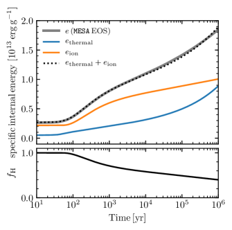
For a star in hydrostatic equilibrium, the virial theorem states that
| (79) |
The right term’s integrand, , is the specific thermal energy of an ideal monatomic ideal gas. Figure 55 shows the total internal energy and gravitational potential energy reported by MESA for the pure-H pre-MS model. On the same scale we show half the total potential energy plus the internal energy. This quantity is not zero; rather, by the virial theorem, it should sum to the non-thermal and non-ideal internal energy (e.g., the ionization energy). This value, recorded from the MESA model, agrees well with our estimate of the ionization energy. Also note that at early times the total energy of the star (internal + potential, not shown) is positive. The phenomenon of positive total energy when ionization energy is included also occurs for envelopes of stars on the asymptotic giant branch (AGB; Paczyński & Ziółkowski, 1968). Figure 56 shows the total energy in the envelope of a MESA model on the AGB. This confirms that the ionization energy is included when MESA reports the total energy of a model.
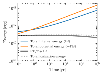
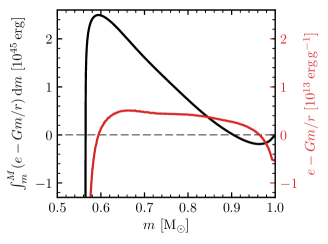
8.5 Latent Heat
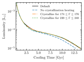
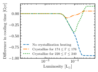
Paper II discusses the inclusion of the latent heat of crystallization for long term WD cooling. Crystallization is a first-order phase transition that manifests in the PC EOS (Potekhin & Chabrier, 2010) as an entropy discontinuity at a plasma coupling parameter of , and can be captured in stellar evolution with in the form of Equation (67). Since the publication of Paper II, controls have been added to MESA to allow smoothing out the injection of latent heat in over a user-specified range of . By default, the range for crystallization is softened to to avoid numerical difficulties with sudden energy injection associated with a sharp transition at . The controls allow for tightening this range for more precise timing on the occurrence of crystallization if necessary. Figure 57 shows the small impact on cooling time for a WD from spreading the latent heat over this broader range of relative to a tighter phase transition for .
The spreading of the phase transition is accomplished by calculating both the liquid and solid solutions within the PC EOS and linearly blending the entropy and internal energy over the specified range of . With expressed in the form of Equation (67), the energy of the phase transition is captured as fluid elements smoothly traverse from liquid-phase to solid-phase. By default MESA automatically switches to using in the form of Equation (67) for . This choice ensures the capture of latent heat release.
Theoretical and observational work has suggested that crystallization in C/O mixtures may occur at higher than the classical one component plasma value of (Horowitz et al., 2007; Winget et al., 2009; Medin & Cumming, 2010; Althaus et al., 2012). Our updated crystallization controls allow for investigating the effect on stellar evolution of crystallization at . Figure 57 shows the potential effects on WD cooling times of varying the for crystallization. Because the heating from crystallization is released very late in the WD evolution, its effects on cooling times are on the order of , and variations in crystallization treatment can lead to changes that are a significant fraction of this timescale.
The composition terms in Equation (59) that were dropped to form Equation (67) are negligible as long as there is no mixing in the crystallization region. Phase separation may violate this assumption and require a modified treatment, but we do not consider this process here. Detailed phase-diagrams for crystallization and the possible associated phase-separation effects are not currently supported in MESA, so our investigation here is limited to the effects of crystallization as a function of a fixed range.
8.6 EOS Blending
As shown in Figure 1 of Paper I, MESA employs a patchwork of several EOSs to provide coverage of a maximal amount of space. When blending from one EOS region into another, care is required to avoid introducing spurious contributions into . At high density, MESA blends from the Helmholtz EOS (HELM, Timmes & Swesty, 2000) for to the PC EOS (Potekhin & Chabrier, 2010) for by default. This default has been changed from the original default of given in Paper I due to the optimal agreement between relevant quantities shown in Figure 59, as explained below. Overall, the two EOSs agree well on thermodynamic quantities in the blending region ( for and ), but Figure 58 shows that the absolute magnitude of the disagreement can still be large enough to influence for a cooling WD when is expressed in the form of Equations (59)–(63).
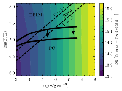
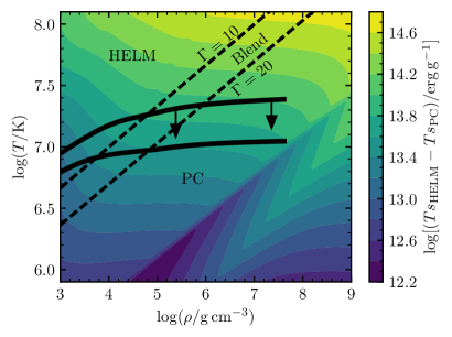
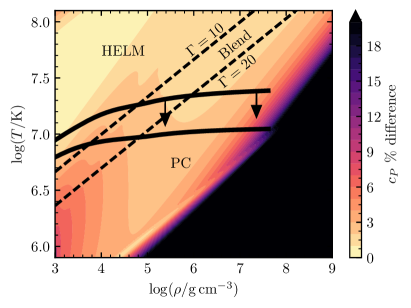
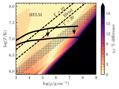
The left panel of Figure 58 indicates that typically the internal energy difference is , while in the region of the blend. As a WD model cools, most of its of mass must eventually pass through this transition. If the energy equation is being solved in the form of Equation (61), of spurious energy would be introduced into the model by EOS blending. Since much of this blending happens after the WD model has cooled to a luminosity of , this extra energy corresponds to of extra WD cooling time.
The default form of given in Equation (65) does not suffer from this spurious heating, since it is expressed in terms of thermodynamic derivatives from the EOS rather than and . For this form of , the differences between or do not directly enter the equations. Instead, changes in with and are tracked with quantities such as and , and Figure 59 shows that these agree well for the EOS blend region. Since the implementation of Equation (65) does not involve any derivatives constructed as finite differences, the fact that quantities such as agree to within a few percent guarantees that will be consistent across the blend, with no significant spurious energy injected due to blending. Crucially, the release of latent heat described in Section 8.5 requires switching to in the form of Equation (67) only for zones with , so both EOS blending and crystallization simultaneously receive appropriate treatments with different forms of in different stellar regions.
8.7 Gravitational Settling
Equation (65) for ignores changes in internal energy due to composition changes. García-Berro et al. (2008) point out that a self-consistent evolutionary approach to WD cooling including the effects of settling requires accounting for composition changes due to element diffusion in . They adopt pure or core compositions with trace and no other isotopes. While this approach is useful for rigorous study of self-consistent WD evolution with diffusion fully coupled to evolution, it is not well suited for a general treatment of realistic mixed core compositions.
MESA splits element diffusion into a separate step before the main structural solve, and hence diffusive effects are not included in . We ensure that the energy associated with settling is not included in by using Equation (65), and we compensate by including an extra heating term in Equation (54). This term is calculated using velocities saved from the element diffusion step as described in Section 3.5. Our results for the effects of settling on WD cooling agree well with García-Berro et al. (2008) and with Deloye & Bildsten (2002) who adopt a heating term similar to our approach.
9 Summary
We explain significant new capabilities and improvements implemented in MESA since the publication of Paper I, Paper II, and Paper III. Progress in the treatment of convective boundaries (Section 2) and element diffusion (Section 3 and Appendix C) will improve studies of their impact on stellar evolution. Advances to MESA in implicit hydrodynamics (Section 4), approximation of 3D RTI effects (Section 5), and coupling with a public version of the STELLA radiative transfer instrument will enhance the modeling of Type IIP SN light curves from post-explosion to post-plateau (Section 6). We integrate these improvements with an exploration of PPISN and black hole formation models (Section 7). Upgrades to estimating the absolute magnitude of a model in a chosen passband (Appendix A), guidance on importing multi-dimensional models into MESA (Appendix B), and new MESA-based software tools (Section D) will strengthen research and education. Input files and related materials for all the figures are available at http://mesastar.org.
Appendix A Colors
We describe MESA’s implementation of bolometric corrections (BCs) for use in estimating the absolute magnitude of a model in a user-chosen filter system. Note this is different than the colors reported by STELLA (Section 6), as the colors module uses pre-computed tables of BCs while STELLA solves the radiative transfer equations on-the-fly (Blinnikov et al., 1998).
The absolute bolometric magnitude () of a star is defined, with reference to the solar absolute bolometric magnitude, as (Torres, 2010):
| (A1) |
where is the absolute bolometric magnitude of the Sun, taken as 4.74 (2015 IAU Resolution B2). This can be transformed into the pass band dependent absolute magnitude, , for a nominal pass band , via
| (A2) |
is the BC for pass band band and accounts for the flux emitted outside of the wavelength range of the filter system. The derivation of a BC requires an atmospheric model of a star such that a stellar spectrum can be computed over all wavelengths, a computationally costly process. To prevent the requirement of actually having to generate a spectra at each time-step, we make use of pre-computed BC tables. These define the BC as a function of the stellar photosphere; , and the metallicity , and are derived from pre-computed grids of stellar atmosphere models, (see e.g., Kurucz, 1970; Husser et al., 2013). Given the parameters at the stellar photosphere, we interpolate each set of BCs over , and using linear interpolation over nearest neighbors and without extrapolation for points outside of the table range.
We provide two sets of pre-processed tables of BCs, though a user may provide their own. From Lejeune et al. (1998) we provide the Johnson-Cousins-Class bands UBVRcIcJHKLL′M. This table provides the BCs over the parameter range , and , with a variable sampling rate. Figure 60 shows the time evolution of the absolute magnitude of a 1 star with the pass bands defined in Lejeune et al. (1998). We also provide a set of blackbody BCs for the pass bands UBVRcIc, over the range in steps of . As these are blackbody corrections there is no or dependence.
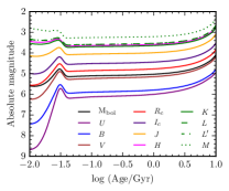
There are many other possibilities for other pass bands or classes of object (Fukugita et al., 1996; Girardi et al., 2002; Bessell, 2011; Bessell & Murphy, 2012). Thus the tables we provide are not a definitive set, but merely a reasonable starting point for modeling stellar objects. Other astrophysical objects like WDs, exoplanets, or SN light curves require calculating specialized tables. Users may provide BC tables defined in terms of , and .
Appendix B Model Relaxation
To simplify the process of importing a model into MESA, we have developed simple relaxation routines that allow the construction of a starting model in hydrostatic equilibrium with specified profiles for composition, angular momentum, and entropy. Examples that motivate importing a model into MESA include multi-dimensional simulations of stellar mergers, common envelope evolution, and the effects of SN explosions on nearby companions.
The relaxation process inputs include 1D profiles of composition and angular momentum. The process also requires either an entropy profile or the profiles of pairs of values , , or , from which MESA extracts the entropy using the eos module. Note that in the case where the entropy is not provided directly, the relaxed model will match the entropy computed by the eos module, but not neccesarily the input , , or profiles. A good match for the input profiles depends on the input data corresponding to a model in hydrostatic equilibrium computed with an EOS that is consistent with MESA’s.
Relaxation is done via pseudo-evolution of a stellar model for which mixing, angular momentum transport, and changes in composition from nuclear burning are suppressed, while a quantity of interest is incrementally altered until it reaches the desired value up to a pre-defined tolerance. Throughout this relaxation process, hydrostatic equilibrium is enforced. The starting stellar model can be any MESA model with the required mass, and for most cases a ZAMS star at works well. The first two steps in the relaxation of a model fix the composition and angular momentum profiles. This is done by directly adjusting the variables for composition and angular momentum of each cell until the desired values are reached. Since the entropy is a derived quantity in MESA, the third step relaxes the entropy indirectly via the energy equation. This is achieved by adding a heating term that injects energy in regions where the entropy is below the target value, and removes energy in regions where the entropy is above the target value. This specific heating rate is
| (B1) |
where , and are the specific internal energy, current entropy, and target entropy respectively at the mass coordinate . The timescale for the relaxation process is specified by . The value should be chosen to be small enough that energy transport is negligible during the pseudo-evolution. In practice, can be chosen to be orders of magnitude smaller than the dynamical timescale of the system.
We verified that using the entropy, composition, and angular momentum profiles of a model computed with MESA as input, the relaxation procedure can reproduce the original model to within . An example is provided in the test suite under the name relax_composition_j_entropy.
We tested these relaxation routines using the outcome of a stellar merger computed with the STARSMASHER101010The STARSMASHER code is open source and freely available at https://jalombar.github.io/starsmasher/ SPH code (Gaburov et al., 2010; Lombardi et al., 2011), configured to use the MESA EOS. Two coeval non-rotating MESA models with ZAMS masses of and are evolved until the star reaches . These models are then imported into STARSMASHER to simulate a head-on collision, such that the relative velocity of the two stars at infinity is zero. We find that of material is lost from the system due to the collision.
We compute spherical mass-weighted averages of the composition, , and . These profiles are input into the MESA relaxation process, along with a zero angular momentum profile since the model is a head-on collision of non-rotating stars. Figure 61 shows that the relaxed model closely follows the input smoothed particle hydrodynamic (SPH) merger model in the central regions, though densities are larger throughout the inner . Density differences of more than an order of magnitude are present in the outer layers. This is a consequence of these layers not being in hydrostatic equilibrium in the input SPH simulation. The MESA relaxation process matches the entropy rather than density profile of the SPH model assuming hydrostatic equilibrium as discussed above. The relaxed model corresponds to the final configuration if it contracts adiabatically, which is a good approximation as velocities in the SPH model are well below the local sound speed (Pan et al., 2013).
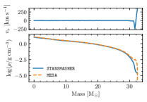
Appendix C Element Diffusion Implementation Details
This appendix provides implementation details not contained in Section 3. Equations (2)–(4) and (LABEL:eq:BurgersMomentum) give the full set of diffusion equations that must be solved to obtain diffusion velocities. For total species in the plasma (including electrons), Equation (LABEL:eq:BurgersMomentum) provides equations (one for each ion species), Equation (2) provides equations (one for each species including electrons), and Equations (3) and (4) each provide one additional equation, for a total of independent equations. The unknowns are diffusion velocities , heat flow vectors , and the electric field .
The inputs provided from the MESA model are the number densities , temperature , gradients of each of these quantities and , species mass in atomic units , species mean charge as an average ionization state , and resistance coefficients , , , (defined in Equation 86 of Paper III). The coefficients are calculated as described in Section 3.3. Together with the mean ionization states, these are the key pieces of input physics that determine the diffusion of all ions. Extra acceleration terms for radiative levitation are either set to zero by default, or calculated as in Hu et al. (2011) when the option to include radiative levitation is enabled.
In the spirit of Thoul et al. (1994), Equations (2)–(4) and (LABEL:eq:BurgersMomentum) are grouped into a single matrix equation:
| (C1) |
The vectors capturing the driving terms are
| (C2) |
| (C3) |
| (C4) |
| (C5) |
The vector containing the unknowns is
| (C6) |
For , the right hand side matrix of Equation (C1) is
| (C7) |
For , the matrix terms are
| (C8) |
For ,
| (C9) |
For ,
| (C10) |
Indices capture the equations (LABEL:eq:BurgersMomentum) for the ions. Indices capture the equations (2). Indices capture the two constraints in Equations (3) and (4).
For a generic driving term that takes the form of an extra force on ions of species , a term appears on the left hand side of Equation (LABEL:eq:BurgersMomentum). This can be accounted for in the matrix setup by adding another vector to the left hand side of Equation (C1) with the form
| (C11) |
One such extra driving force that may be explored with MESA in the future is Coulomb separation in dense matter arising from non-ideal corrections for the ions (Chang et al., 2010; Beznogov & Yakovlev, 2013; Diaw & Murillo, 2016).
The diffusion velocities are separated into two terms capturing the distinct effects of gravitational settling and ordinary diffusion in the tradition of Equation (11) of Iben & MacDonald (1985):
| (C12) |
where following the notation of Thoul et al. (1994). These separate terms are constructed by inverting the matrix and then solving Equation (C1) for just one of , , , and at a time on the left hand side. These results can then be linearly combined to construct and such that the the full sum in Equation (C12) gives a solution that satisfies the complete set represented by Equation (C1).
When electrons become degenerate, we drop all Equations (2) and set the heat flow vectors to . Equation (C1) then represents a system of just equations and the vectors and matrices simplify considerably, dropping all entries for indices or in the definitions given in Equations (C2)–(C10). To avoid discontinuities, we employ a blend that smoothly transitions between the diffusion velocity solutions over a range in , where is the electron chemical potential. By default, the blend is centered around , with user controls available to adjust the range of this blending region.
Appendix D Software Infrastructure
Software is an integral enabler of observation, theory, and computation and a primary modality for realizing the discoveries and innovations expressed, for example, in the astronomy and astrophysics decadal surveys (e.g., National Research Council, 1991; National Research Council, 2001, 2011). In this appendix we describe new software stacks at a variety of scales that enhance the research and education infrastructure.
D.1 Not A Number
Not a Number (NaN) is a numeric data type representing an undefined or unrepresentable value (e.g., Goldberg, 1991; Hauser, 1996). Examples include and in real arithmetic. In the IEEE 754 floating-point standard (IEEE, 2008) there are two types of NaNs: quiet (qNaN) and signaling (sNaN). A qNaN propagates errors resulting from invalid operations or values without triggering a floating point exception. An sNaN precipitates an invalid operation exception whenever an attempt is made to use one as an arithmetic operand. The IEEE 754 standard requires qNaN as the default, while an sNaN can be used to support features such as filling uninitialized memory or other extensions to floating-point arithmetic.
NaN and infinity (INF) setting and testing routines are provided within the utils_nan.f90 file. A consistent set of interfaces allows for initializing scalars/arrays to NaN values, and testing for qNaN, sNaN, or INF values. Interface overloading allows handling of single, double or quad precision scalars or arrays of rank between 1 and 4. This module provides four generic interfaces. Logical function is_nan(x,signal) returns true if x contains NaNs and false otherwise. The optional logical argument signal determines whether qNaN, sNaN or both are tested for. Logical function is_inf(x) returns true if x contains INFs and false otherwise. Logical function is_bad(x) returns true if x contains NaN or INF values and false otherwise. Routine set_nan(x,signal) sets a scalar or array x to NaN values. The optional logical argument signal determines whether a qNaN or sNaN is set.
The library framework of MESA is designed to be interoperable within other software ecosystems. For example, these NaN and INF interfaces are of potential interest to users of MESA or developers of similar software instruments.
D.2 MESA-Web
Stellar evolution software instruments can be complicated to install and use, especially when the aim is primarily pedagogical (e.g., high-school or undergraduate courses). Motivated by the community’s expressed need for a lower barrier to entry for education, a web-based interface to MESA was developed, MESA-Web at http://mesa-web.asu.edu. MESA-Web currently allows choices for the initial mass, metallicity, rotation, mass loss, nuclear reaction network, custom nuclear reactions rates, spatial and temporal resolution, and model output rate.
MESA-Web sends the user an email message when their job has completed that contains a URL of a zip file to download. The unzipped output directory contains a MESA history data file holding the time evolution of 57 quantities, as well as a series of MESA profile data files containing information on 56 quantities in each zone of the stellar model at discrete model numbers. Also included in the output is an MP4 formatted video containing a plot dashboard of the abundance profiles, Kippenhahn diagram, Hertzsprung-Russell Diagram, rotational profile, and temperature, density, and pressure profiles.
MESA-Web is currently hosted on a 4-core server at Arizona State University and allows jobs to run on a single core for 4 hours of walltime or until the model reaches iron core collapse. Launched in June 2015, MESA-Web has presently served more than 3000 models to over 600 different users at over 40 academic institutions. Efforts to expand MESA-Web’s capabilities include porting the service to a host with enhanced compute resources, simulating core-collapse supernova explosions (see Paper III) and light curves (see Section 6), and binary star evolution (see Paper III).
D.3 MESA-Docker
Docker is a software technology designed to deploy and run applications by using “containers”. Containers provide much of the virtualization power of traditional virtual machines while requiring far less resource overhead. This allows efficient packaging of an entire operating environment, with all of the necessary libraries and other dependencies for a large software tool such as MESA. The MESA-Docker package (Bauer & Farmer, 2017) provides a solution that simplifies the requirements for locally running a full MESA installation with all capabilities available, with only minor overhead associated with running in a container. MESA-Docker will be useful for new users, students with educational projects, and Windows operating system users.
D.4 pyMESA
pyMESA (Farmer, 2017) allows embedding of MESA modules into Python projects. pyMESA currently supports using the equation of state (eos), nuclear reaction (rates), neutrino (neu), atmosphere (atm), and opacity (kap) packages. This software infrastructure will be useful for users who want to use parts of MESA in their own Python software projects. As an example of these capabilities, Figures 58 and 59 were produced using the pyMESA eos interface to make direct calls to the MESA EOS routines.
D.5 MESAstar Model Optimization
The MESAstar test suite contains a sample case that shows how to use the simplex optimization algorithm (Nelder & Mead, 1965) to find stellar models that minimize a specified by automatically adjusting a variety of control parameters.111111This is the same simplex algorithm that is used for finding matches in asteroseismology applications using MESA (see Paper III, Section 3). The code reported here is a simplified subset of that tool and is now easier to use and adapt to new problems. The to be minimized can contain both pre-supplied and user-defined terms. Pre-supplied terms include , , , , surface , surface , and age. An easy-to-use framework allows the user to define other terms to include in the . Control parameters include , , , , and . Other stellar evolution parameters can be easily added from the extensive set of controls in MESA. We provide a MESA test suite case using this new capability to calibrate a solar model. This can serve as a template for users wishing to use this method to search for models that match the observed properties of specific stars.
D.6 http://mesastar.org
Reproducibility is bedrock to scientific research. Provenance, as the term relates to software instruments (Van den Bussche & Vianu, 2001; Carata et al., 2014), is the ability to record the full history of a result. Scientific research is generally held to be of good provenance when it is documented in detail sufficient to allow reproducibility. The MESA project facilitates provenance by the research community in four ways. One, by curating public releases of the source code, makefiles, test suite, and how the source code was compiled GNU compilers are redistributed in the MESA Software Development Kit (see Paper II) at http://mesa.sourceforge.net. Two, by providing bit-for-bit consistency for all results across all the supported platforms (see Paper III). Three, by supporting a user mailing-list to openly share knowledge (see the Manifesto in Paper I). Currently, over 12,000 messages are archived and searchable. Four, by hosting a web-portal at http://mesastar.org to share MESA-oriented software contributions and reposit the MESA files (inlist, run_star_extra.f, etc) that specify all the ingredients needed to reproduce a scientific result. Currently, http://mesastar.org offers over 120 MESA-oriented software contributions and inlist repositories.
References
- Abbott et al. (2016a) Abbott, B. P., Abbott, R., Abbott, T. D., et al. 2016a, Physical Review Letters, 116, 061102
- Abbott et al. (2016b) —. 2016b, ApJ, 818, L22
- Abbott et al. (2016c) —. 2016c, Phys. Rev. Lett., 116, 241103
- Abbott et al. (2016d) —. 2016d, ApJ, 832, L21
- Abbott et al. (2016e) —. 2016e, ApJ, 833, L1
- Abbott et al. (2016f) —. 2016f, ApJS, 227, 14
- Abbott et al. (2017a) —. 2017a, ApJ, 839, 12
- Abbott et al. (2017b) —. 2017b, Phys. Rev. Lett., 119, 141101
- Althaus & Benvenuto (2000) Althaus, L. G., & Benvenuto, O. G. 2000, MNRAS, 317, 952
- Althaus et al. (2012) Althaus, L. G., García-Berro, E., Isern, J., Córsico, A. H., & Miller Bertolami, M. M. 2012, A&A, 537, A33
- Althaus et al. (2013) Althaus, L. G., Miller Bertolami, M. M., & Córsico, A. H. 2013, A&A, 557, A19
- Althaus et al. (2001) Althaus, L. G., Serenelli, A. M., & Benvenuto, O. G. 2001, MNRAS, 323, 471
- Althaus et al. (2003) Althaus, L. G., Serenelli, A. M., Córsico, A. H., & Montgomery, M. H. 2003, A&A, 404, 593
- Arcavi et al. (2014) Arcavi, I., Gal-Yam, A., Sullivan, M., et al. 2014, ApJ, 793, 38
- Arcoragi & Fontaine (1980) Arcoragi, J.-P., & Fontaine, G. 1980, ApJ, 242, 1208
- Arnett (1969) Arnett, W. D. 1969, Ap&SS, 5, 180
- Arzoumanian et al. (2014) Arzoumanian, Z., Gendreau, K. C., Baker, C. L., et al. 2014, in Proc. SPIE, Vol. 9144, Space Telescopes and Instrumentation 2014: Ultraviolet to Gamma Ray, 914420
- Bade et al. (1996) Bade, N., Komossa, S., & Dahlem, M. 1996, A&A, 309, L35
- Baklanov et al. (2005) Baklanov, P. V., Blinnikov, S. I., & Pavlyuk, N. N. 2005, Astronomy Letters, 31, 429
- Barkat et al. (1967) Barkat, Z., Rakavy, G., & Sack, N. 1967, Phys. Rev. Lett., 18, 379
- Batta et al. (2017) Batta, A., Ramirez-Ruiz, E., & Fryer, C. 2017, ApJ, 846, L15
- Batten et al. (1997) Batten, P., Leschziner, M. A., & Goldberg, U. C. 1997, JCoPh, 137, 38
- Bauer & Farmer (2017) Bauer, E. B., & Farmer, R. 2017, evbauer/MESA-Docker: MESA 10108, Zenodo, doi:10.5281/zenodo.1002850
- Benz & Thielemann (1990) Benz, W., & Thielemann, F.-K. 1990, ApJ, 348, L17
- Bersten et al. (2011) Bersten, M. C., Benvenuto, O., & Hamuy, M. 2011, ApJ, 729, 61
- Bessell & Murphy (2012) Bessell, M., & Murphy, S. 2012, PASP, 124, 140
- Bessell (2011) Bessell, M. S. 2011, PASP, 123, 1442
- Beznogov et al. (2016) Beznogov, M. V., Fortin, M., Haensel, P., Yakovlev, D. G., & Zdunik, J. L. 2016, MNRAS, 463, 1307
- Beznogov & Yakovlev (2013) Beznogov, M. V., & Yakovlev, D. G. 2013, Phys. Rev. Lett., 111, 161101
- Bildsten & Hall (2001) Bildsten, L., & Hall, D. M. 2001, ApJ, 549, L219
- Blinnikov & Sorokina (2004) Blinnikov, S., & Sorokina, E. 2004, Ap&SS, 290, 13
- Blinnikov et al. (1998) Blinnikov, S. I., Eastman, R., Bartunov, O. S., Popolitov, V. A., & Woosley, S. E. 1998, ApJ, 496, 454
- Blinnikov & Panov (1996) Blinnikov, S. I., & Panov, I. V. 1996, Astronomy Letters, 22, 39
- Blinnikov et al. (2006) Blinnikov, S. I., Röpke, F. K., Sorokina, E. I., et al. 2006, A&A, 453, 229
- Böhm-Vitense (1958) Böhm-Vitense, E. 1958, ZAp, 46, 108
- Bossini et al. (2015) Bossini, D., Miglio, A., Salaris, M., et al. 2015, MNRAS, 453, 2290
- Brayton et al. (1972) Brayton, R. K., Gustavson, F. G., & Hachtel, G. D. 1972, Proceedings of the IEEE, 60, 98
- Brugière (2017) Brugière, T. 2017, Nuclear Instruments and Methods in Physics Research A, 845, 326
- Burgers (1969) Burgers, J. M. 1969, Flow Equations for Composite Gases (Academic Press, New York)
- Cao et al. (2013) Cao, Y., Kasliwal, M. M., Arcavi, I., et al. 2013, ApJ, 775, L7
- Caputo et al. (1989) Caputo, F., Chieffi, A., Tornambe, A., Castellani, V., & Pulone, L. 1989, ApJ, 340, 241
- Carata et al. (2014) Carata, L., Akoush, S., Balakrishnan, N., et al. 2014, Queue, 12, 10
- Cassisi et al. (2003) Cassisi, S., Salaris, M., & Irwin, A. W. 2003, ApJ, 588, 862
- Castellani et al. (1985) Castellani, V., Chieffi, A., Tornambe, A., & Pulone, L. 1985, ApJ, 296, 204
- Castellani et al. (1971) Castellani, V., Giannone, P., & Renzini, A. 1971, Ap&SS, 10, 355
- Castor (1970) Castor, J. I. 1970, MNRAS, 149, 111
- Chang & Bildsten (2003) Chang, P., & Bildsten, L. 2003, ApJ, 585, 464
- Chang & Bildsten (2004) —. 2004, ApJ, 605, 830
- Chang et al. (2010) Chang, P., Bildsten, L., & Arras, P. 2010, ApJ, 723, 719
- Chatzopoulos & Wheeler (2012) Chatzopoulos, E., & Wheeler, J. C. 2012, ApJ, 760, 154
- Chatzopoulos et al. (2013) Chatzopoulos, E., Wheeler, J. C., & Couch, S. M. 2013, ApJ, 776, 129
- Cheng & Shu (2007) Cheng, J., & Shu, C.-W. 2007, JCoPh, 227, 1567
- Cheng & Shu (2014) —. 2014, JCoPh, 257, 143
- Cheng et al. (2012) Cheng, J., Shu, C.-W., & Zeng, Q. 2012, Communications in Computational Physics, 12, 1307
- Chevalier (1976) Chevalier, R. A. 1976, ApJ, 207, 872
- Chevalier & Klein (1978) Chevalier, R. A., & Klein, R. I. 1978, ApJ, 219, 994
- Christensen-Dalsgaard (2008) Christensen-Dalsgaard, J. 2008, Ap&SS, 316, 113
- Christensen-Dalsgaard & Thompson (2011) Christensen-Dalsgaard, J., & Thompson, M. J. 2011, in IAU Symposium, Vol. 271, IAU Symposium, ed. N. H. Brummell, A. S. Brun, M. S. Miesch, & Y. Ponty, 32–61
- Clausen et al. (2015) Clausen, D., Piro, A. L., & Ott, C. D. 2015, ApJ, 799, 190
- Constantino et al. (2015) Constantino, T., Campbell, S. W., Christensen-Dalsgaard, J., Lattanzio, J. C., & Stello, D. 2015, MNRAS, 452, 123
- Constantino et al. (2017) Constantino, T., Campbell, S. W., & Lattanzio, J. C. 2017, MNRAS, 472, 4900
- Constantino et al. (2016) Constantino, T., Campbell, S. W., Lattanzio, J. C., & van Duijneveldt, A. 2016, MNRAS, 456, 3866
- Couch et al. (2015) Couch, S. M., Chatzopoulos, E., Arnett, W. D., & Timmes, F. X. 2015, ApJ, 808, L21
- Coughlin et al. (2017) Coughlin, E. R., Quataert, E., Fernández, R., & Kasen, D. 2017, ArXiv e-prints, arXiv:1710.01746
- Cox & Giuli (1968) Cox, J. P., & Giuli, R. T. 1968, Principles of Stellar Structure (Gordon and Breach, New York)
- Creevey et al. (2015) Creevey, O. L., Thévenin, F., Berio, P., et al. 2015, A&A, 575, A26
- Cristini et al. (2017) Cristini, A., Meakin, C., Hirschi, R., et al. 2017, MNRAS, 471, 279
- Daligault et al. (2016) Daligault, J., Baalrud, S. D., Starrett, C. E., Saumon, D., & Sjostrom, T. 2016, Phys. Rev. Lett., 116, 075002
- de Dinechin et al. (2007) de Dinechin, F., Lauter, C., & Muller, J.-M. 2007, RAIRO-Theor. Inf. Appl., 41, 85
- de Jager et al. (1988) de Jager, C., Nieuwenhuijzen, H., & van der Hucht, K. A. 1988, A&AS, 72, 259
- deBoer et al. (2017) deBoer, R. J., Görres, J., Wiescher, M., et al. 2017, Reviews of Modern Physics, 89, 035007
- Deloye & Bildsten (2002) Deloye, C. J., & Bildsten, L. 2002, ApJ, 580, 1077
- Dessart et al. (2017) Dessart, L., Hillier, D., & Audit, E. 2017, A&A, 605, A83
- Dessart & Hillier (2010) Dessart, L., & Hillier, D. J. 2010, MNRAS, 405, 2141
- Dessart & Hillier (2011) —. 2011, MNRAS, 410, 1739
- Dessart et al. (2013) Dessart, L., Hillier, D. J., Waldman, R., & Livne, E. 2013, MNRAS, 433, 1745
- Dessart et al. (2015) Dessart, L., Hillier, D. J., Woosley, S., et al. 2015, MNRAS, 453, 2189
- Diaw & Murillo (2016) Diaw, A., & Murillo, M. S. 2016, ApJ, 829, 16
- Duffell (2016) Duffell, P. C. 2016, ApJ, 821, 76
- Duffell & MacFadyen (2011) Duffell, P. C., & MacFadyen, A. I. 2011, ApJS, 197, 15
- Eastman & Pinto (1993) Eastman, R. G., & Pinto, P. A. 1993, ApJ, 412, 731
- Eastman et al. (1994) Eastman, R. G., Woosley, S. E., Weaver, T. A., & Pinto, P. A. 1994, ApJ, 430, 300
- Eggleton (1972) Eggleton, P. P. 1972, MNRAS, 156, 361
- Eldridge & Tout (2004) Eldridge, J. J., & Tout, C. A. 2004, MNRAS, 353, 87
- Ergon et al. (2015) Ergon, M., Jerkstrand, A., Sollerman, J., et al. 2015, A&A, 580, A142
- Farmer (2017) Farmer, R. 2017, rjfarmer/pyMesa v1.0.0, zenodo, doi:10.5281/zenodo.846305
- Farmer et al. (2016) Farmer, R., Fields, C. E., Petermann, I., et al. 2016, ApJS, 227, 22
- Farmer et al. (2015) Farmer, R., Fields, C. E., & Timmes, F. X. 2015, ApJ, 807, 184
- Fields et al. (2017) Fields, C. E., Timmes, F. X., Farmer, R. J., Petermann, I., & Couch, S. M. 2017, In prep.
- Fowler & Hoyle (1964) Fowler, W. A., & Hoyle, F. 1964, ApJS, 9, 201
- Fraley (1968) Fraley, G. S. 1968, Ap&SS, 2, 96
- Fremling et al. (2014) Fremling, C., Sollerman, J., Taddia, F., et al. 2014, A&A, 565, A114
- Fryer et al. (2002) Fryer, C. L., Holz, D. E., & Hughes, S. A. 2002, ApJ, 565, 430
- Fryer & Kalogera (2001) Fryer, C. L., & Kalogera, V. 2001, ApJ, 554, 548
- Fryer et al. (2001) Fryer, C. L., Woosley, S. E., & Heger, A. 2001, ApJ, 550, 372
- Fryxell et al. (2000) Fryxell, B., Olson, K., Ricker, P., et al. 2000, ApJS, 131, 273
- Fukugita et al. (1996) Fukugita, M., Ichikawa, T., Gunn, J. E., et al. 1996, AJ, 111, 1748
- Gabriel et al. (2014) Gabriel, M., Noels, A., Montalbán, J., & Miglio, A. 2014, A&A, 569, A63
- Gaburov et al. (2010) Gaburov, E., Lombardi, Jr., J. C., & Portegies Zwart, S. 2010, MNRAS, 402, 105
- Gaia Collaboration et al. (2016a) Gaia Collaboration, Prusti, T., de Bruijne, J. H. J., et al. 2016a, A&A, 595, A1
- Gaia Collaboration et al. (2016b) Gaia Collaboration, Brown, A. G. A., Vallenari, A., et al. 2016b, A&A, 595, A2
- García-Berro et al. (2008) García-Berro, E., Althaus, L. G., Córsico, A. H., & Isern, J. 2008, ApJ, 677, 473
- García-Berro et al. (2010) García-Berro, E., Torres, S., Althaus, L. G., et al. 2010, Nature, 465, 194
- Gear (1971) Gear, C. W. 1971, Numerical initial value problems in ordinary differential equations, Prentice-Hall Series in Automatic Computation (Prentice-Hall, Engelwood Cliffs)
- Gehmeyr et al. (1997) Gehmeyr, M., Cheng, B., & Mihalas, D. 1997, Shock Waves, 7, 255
- Gehmeyr & Mihalas (1994) Gehmeyr, M., & Mihalas, D. 1994, Physica D Nonlinear Phenomena, 77, 320
- Gendreau et al. (2012) Gendreau, K. C., Arzoumanian, Z., & Okajima, T. 2012, in Proc. SPIE, Vol. 8443, Space Telescopes and Instrumentation 2012: Ultraviolet to Gamma Ray, 844313
- Gendreau et al. (2016) Gendreau, K. C., Arzoumanian, Z., Adkins, P. W., et al. 2016, in Proc. SPIE, Vol. 9905, Space Telescopes and Instrumentation 2016: Ultraviolet to Gamma Ray, 99051H
- Ghosh et al. (2017) Ghosh, S., Chatterjee, D., Kaplan, D. L., Brady, P. R., & Van Sistine, A. 2017, PASP, 129, 114503
- Girardi et al. (2002) Girardi, L., Bertelli, G., Bressan, A., et al. 2002, A&A, 391, 195
- Goldberg (1991) Goldberg, D. 1991, ACM Comput. Surv., 23, 5
- Gossan et al. (2016) Gossan, S. E., Sutton, P., Stuver, A., et al. 2016, Phys. Rev. D, 93, 042002
- Hammer et al. (2010) Hammer, N. J., Janka, H.-T., & Müller, E. 2010, ApJ, 714, 1371
- Hansen et al. (2004) Hansen, C. J., Kawaler, S. D., & Trimble, V. 2004, Stellar interiors : physical principles, structure, and evolution (New York: Springer-Verlag)
- Hauser (1996) Hauser, J. R. 1996, ACM Trans. Program. Lang. Syst., 18, 139
- Heger et al. (2003) Heger, A., Fryer, C. L., Woosley, S. E., Langer, N., & Hartmann, D. H. 2003, ApJ, 591, 288
- Herant & Benz (1991) Herant, M., & Benz, W. 1991, ApJ, 370, L81
- Hirata et al. (1987) Hirata, K., Kajita, T., Koshiba, M., Nakahata, M., & Oyama, Y. 1987, Phys. Rev. Lett., 58, 1490
- Hollands et al. (2017) Hollands, M. A., Koester, D., Alekseev, V., Herbert, E. L., & Gänsicke, B. T. 2017, MNRAS, 467, 4970
- Horowitz et al. (2007) Horowitz, C. J., Berry, D. K., & Brown, E. F. 2007, Phys. Rev. E, 75, 066101
- Hu et al. (2011) Hu, H., Tout, C. A., Glebbeek, E., & Dupret, M.-A. 2011, MNRAS, 418, 195
- Hunter (2007) Hunter, J. D. 2007, Computing In Science & Engineering, 9, 90
- Husser et al. (2013) Husser, T.-O., Wende-von Berg, S., Dreizler, S., et al. 2013, A&A, 553, A6
- Iben et al. (1992) Iben, Jr., I., Fujimoto, M. Y., & MacDonald, J. 1992, ApJ, 388, 521
- Iben & MacDonald (1985) Iben, Jr., I., & MacDonald, J. 1985, ApJ, 296, 540
- IEEE (2008) IEEE. 2008, IEEE Std 754-2008, 1
- Istrate et al. (2016a) Istrate, A. G., Fontaine, G., Gianninas, A., et al. 2016a, A&A, 595, L12
- Istrate et al. (2016b) Istrate, A. G., Marchant, P., Tauris, T. M., et al. 2016b, A&A, 595, A35
- Janka (2017) Janka, H.-T. 2017, ArXiv e-prints, arXiv:1702.08713
- Kamm & Timmes (2007) Kamm, J. R., & Timmes, F. X. 2007, On Efficient Generation of Numerically Robust Sedov Solutions, Tech. Rep. Technical Report LA-UR-07-2849, Los Alamos National Laboratory
- Käppeli & Mishra (2014) Käppeli, R., & Mishra, S. 2014, JCoPh, 259, 199
- Kasen et al. (2006) Kasen, D., Thomas, R. C., & Nugent, P. 2006, ApJ, 651, 366
- Kasen & Woosley (2009) Kasen, D., & Woosley, S. E. 2009, ApJ, 703, 2205
- Kasen et al. (2011) Kasen, D., Woosley, S. E., & Heger, A. 2011, ApJ, 734, 102
- Kippenhahn et al. (1965) Kippenhahn, R., Thomas, H. C., & Weigert, A. 1965, ZAp, 61, 241
- Kippenhahn et al. (2012) Kippenhahn, R., Weigert, A., & Weiss, A. 2012, Stellar Structure and Evolution, Astronomy and Astrophysics Library (Berlin, Heidelberg: Springer-Verlag), doi:10.1007/978-3-642-30304-3
- Kluyver et al. (2016) Kluyver, T., Ragan-Kelley, B., Pérez, F., et al. 2016, in Positioning and Power in Academic Publishing: Players, Agents and Agendas: Proceedings of the 20th International Conference on Electronic Publishing, IOS Press, 87
- Koester (2009) Koester, D. 2009, A&A, 498, 517
- Komossa (2015) Komossa, S. 2015, Journal of High Energy Astrophysics, 7, 148
- Korol et al. (2017) Korol, V., Rossi, E. M., Groot, P. J., et al. 2017, MNRAS, 470, 1894
- Kulkarni (2016) Kulkarni, S. R. 2016, in American Astronomical Society Meeting Abstracts, Vol. 227, American Astronomical Society Meeting Abstracts, 314.01
- Kurucz (1970) Kurucz, R. L. 1970, SAO Special Report, 309
- Kurucz & Bell (1995) Kurucz, R. L., & Bell, B. 1995, Atomic line list (Smithsonian Astrophysical Observatory, Cambridge, MA)
- Laher et al. (2017) Laher, R. R., Masci, F. J., Groom, S., et al. 2017, ArXiv e-prints, arXiv:1708.01584
- Langer et al. (1985) Langer, N., El Eid, M. F., & Fricke, K. J. 1985, A&A, 145, 179
- Law et al. (2009) Law, N. M., Kulkarni, S. R., Dekany, R. G., et al. 2009, PASP, 121, 1395
- Lejeune et al. (1998) Lejeune, T., Cuisinier, F., & Buser, R. 1998, A&AS, 130, 65
- Li (2014) Li, Y.-F. 2014, in International Journal of Modern Physics Conference Series, Vol. 31, International Journal of Modern Physics Conference Series, 1460300
- Limongi (2017) Limongi, M. 2017, ArXiv e-prints, arXiv:1706.01913
- Limongi & Chieffi (2003) Limongi, M., & Chieffi, A. 2003, ApJ, 592, 404
- Limongi & Chieffi (2006) —. 2006, ApJ, 647, 483
- Limongi et al. (2000) Limongi, M., Straniero, O., & Chieffi, A. 2000, ApJS, 129, 625
- Lindegren et al. (2016) Lindegren, L., Lammers, U., Bastian, U., et al. 2016, A&A, 595, A4
- Lombardi et al. (2011) Lombardi, Jr., J. C., Holtzman, W., Dooley, K. L., et al. 2011, ApJ, 737, 49
- Lovegrove & Woosley (2013) Lovegrove, E., & Woosley, S. E. 2013, ApJ, 769, 109
- LSST Science Collaboration et al. (2017) LSST Science Collaboration, Marshall, P., Anguita, T., et al. 2017, ArXiv e-prints, arXiv:1708.04058
- Marchant et al. (2016) Marchant, P., Langer, N., Podsiadlowski, P., Tauris, T. M., & Moriya, T. J. 2016, A&A, 588, A50
- Matzner & McKee (1999) Matzner, C. D., & McKee, C. F. 1999, ApJ, 510, 379
- Medin & Cumming (2010) Medin, Z., & Cumming, A. 2010, Phys. Rev. E, 81, 036107
- Michaud et al. (2015) Michaud, G., Alecian, G., & Richer, J. 2015, Atomic Diffusion in Stars, Astronomy and Astrophysics Library (Springer International Publishing, Switzerland), doi:10.1007/978-3-319-19854-5
- Michaud et al. (2007) Michaud, G., Richer, J., & Richard, O. 2007, ApJ, 670, 1178
- Mihalas (1978) Mihalas, D. 1978, Stellar atmospheres (2nd ed.; San Francisco: W. H. Freeman and Co.)
- Miller (2016) Miller, M. C. 2016, ApJ, 822, 27
- Misch & Fuller (2016) Misch, G. W., & Fuller, G. M. 2016, Phys. Rev. C, 94, 055808
- Moore & Garaud (2016) Moore, K., & Garaud, P. 2016, ApJ, 817, 54
- Moriya et al. (2013) Moriya, T. J., Blinnikov, S. I., Baklanov, P. V., Sorokina, E. I., & Dolgov, A. D. 2013, MNRAS, 430, 1402
- Morozova et al. (2016) Morozova, V., Piro, A. L., Renzo, M., & Ott, C. D. 2016, ApJ, 829, 109
- Morozova et al. (2015) Morozova, V., Piro, A. L., Renzo, M., et al. 2015, ApJ, 814, 63
- Morozova et al. (2017a) Morozova, V., Piro, A. L., & Valenti, S. 2017a, ApJ, 838, 28
- Morozova et al. (2017b) —. 2017b, ArXiv e-prints, arXiv:1709.04928
- Müller et al. (2016) Müller, B., Heger, A., Liptai, D., & Cameron, J. B. 2016, MNRAS, 460, 742
- Nadezhin (1980) Nadezhin, D. K. 1980, Ap&SS, 69, 115
- National Research Council (1991) National Research Council. 1991, The Decade of Discovery in Astronomy and Astrophysics (Washington DC : National Academy Press)
- National Research Council (2001) —. 2001, Astronomy and Astrophysics in the New Millennium (Washington DC : National Academy Press)
- National Research Council (2011) —. 2011, New Worlds, New Horizons (Washington DC : National Academy Press)
- Nelder & Mead (1965) Nelder, J. A., & Mead, R. 1965, Comput. J, 7, 308
- Nieuwenhuijzen & de Jager (1990) Nieuwenhuijzen, H., & de Jager, C. 1990, A&A, 231, 134
- Noh (1987) Noh, W. F. 1987, JCoPh, 72, 78
- Ober et al. (1983) Ober, W. W., El Eid, M. F., & Fricke, K. J. 1983, A&A, 119, 61
- O’Connor & Ott (2011) O’Connor, E., & Ott, C. D. 2011, ApJ, 730, 70
- Odrzywolek (2009) Odrzywolek, A. 2009, Phys. Rev. C, 80, 045801
- Oluseyi et al. (2012) Oluseyi, H. M., Becker, A. C., Culliton, C., et al. 2012, AJ, 144, 9
- Özel et al. (2016) Özel, F., Psaltis, D., Arzoumanian, Z., Morsink, S., & Bauböck, M. 2016, ApJ, 832, 92
- Paczyński & Ziółkowski (1968) Paczyński, B., & Ziółkowski, J. 1968, Acta Astron., 18, 255
- Pan et al. (2013) Pan, K.-C., Ricker, P. M., & Taam, R. E. 2013, ApJ, 773, 49
- Paquette et al. (1986a) Paquette, C., Pelletier, C., Fontaine, G., & Michaud, G. 1986a, ApJS, 61, 177
- Paquette et al. (1986b) —. 1986b, ApJS, 61, 197
- Patton et al. (2017a) Patton, K. M., Lunardini, C., & Farmer, R. J. 2017a, ApJ, 840, 2
- Patton et al. (2017b) Patton, K. M., Lunardini, C., Farmer, R. J., & Timmes, F. X. 2017b, ApJ, 851, 6
- Paxton et al. (2011) Paxton, B., Bildsten, L., Dotter, A., et al. 2011, ApJS, 192
- Paxton et al. (2013) Paxton, B., Cantiello, M., Arras, P., et al. 2013, ApJS, 208
- Paxton et al. (2015) Paxton, B., Marchant, P., Schwab, J., et al. 2015, ApJS, 220, 15
- Pejcha & Prieto (2015a) Pejcha, O., & Prieto, J. L. 2015a, ApJ, 799, 215
- Pejcha & Prieto (2015b) —. 2015b, ApJ, 806, 225
- Pérez & Granger (2007) Pérez, F., & Granger, B. E. 2007, Computing in Science & Engineering, 9, 21
- Petermann et al. (2017) Petermann, I., Timmes, F. X., Fields, C. E., & Farmer, R. J. 2017, In preparation
- Popov (1993) Popov, D. V. 1993, ApJ, 414, 712
- Potekhin & Chabrier (2010) Potekhin, A. Y., & Chabrier, G. 2010, Contributions to Plasma Physics, 50, 82
- Quataert et al. (2016) Quataert, E., Fernández, R., Kasen, D., Klion, H., & Paxton, B. 2016, MNRAS, 458, 1214
- Rakavy & Shaviv (1967) Rakavy, G., & Shaviv, G. 1967, ApJ, 148, 803
- Rakavy et al. (1967) Rakavy, G., Shaviv, G., & Zinamon, Z. 1967, ApJ, 150, 131
- Renzo et al. (2017) Renzo, M., Ott, C. D., Shore, S. N., & de Mink, S. E. 2017, A&A, 603, A118
- Ricker et al. (2016) Ricker, G. R., Vanderspek, R., Winn, J., et al. 2016, in Proc. SPIE, Vol. 9904, Space Telescopes and Instrumentation 2016: Optical, Infrared, and Millimeter Wave, 99042B
- Rider (2000) Rider, W. J. 2000, Journal of Computational Physics, 162, 395
- Roxburgh (1978) Roxburgh, I. W. 1978, A&A, 65, 281
- Sacco et al. (2015) Sacco, G. G., Jeffries, R. D., Randich, S., et al. 2015, A&A, 574, L7
- Salaris & Cassisi (2017) Salaris, M., & Cassisi, S. 2017, Royal Society Open Science, 4, 170192
- Scannapieco et al. (2005) Scannapieco, E., Madau, P., Woosley, S., Heger, A., & Ferrara, A. 2005, ApJ, 633, 1031
- Shaffer et al. (2017) Shaffer, N. R., Baalrud, S. D., & Daligault, J. 2017, Phys. Rev. E, 95, 013206
- Smartt (2009a) Smartt, S. J. 2009a, ARA&A, 47, 63
- Smartt (2009b) —. 2009b, ARA&A, 47, 63
- Smartt (2015) —. 2015, PASA, 32, 16
- Smith et al. (2016) Smith, N., Andrews, J. E., & Mauerhan, J. C. 2016, MNRAS, 463, 2904
- Sobolev (1960) Sobolev, V. V. 1960, Moving envelopes of stars ( Cambridge: Harvard University Press)
- Spiro et al. (2014) Spiro, S., Pastorello, A., Pumo, M. L., et al. 2014, MNRAS, 439, 2873
- Stabrowski (1997) Stabrowski, M. M. 1997, Simulation Practice and Theory, 5, 333
- Stanton & Murillo (2016) Stanton, L. G., & Murillo, M. S. 2016, Phys. Rev. E, 93, 043203
- Stern et al. (2004) Stern, D., van Dokkum, P. G., Nugent, P., et al. 2004, ApJ, 612, 690
- Sukhbold et al. (2016a) Sukhbold, T., Ertl, T., Woosley, S. E., Brown, J. M., & Janka, H.-T. 2016a, ApJ, 821, 38
- Sukhbold et al. (2016b) —. 2016b, ApJ, 821, 38
- Sukhbold & Woosley (2014) Sukhbold, T., & Woosley, S. E. 2014, ApJ, 783, 10
- Sullivan et al. (2015) Sullivan, P. W., Winn, J. N., Berta-Thompson, Z. K., et al. 2015, ApJ, 809, 77
- Sullivan et al. (2017) —. 2017, ApJ, 837, 99
- Swartz et al. (1995) Swartz, D. A., Sutherland, P. G., & Harkness, R. P. 1995, ApJ, 446, 766
- Takáts et al. (2014) Takáts, K., Pumo, M. L., Elias-Rosa, N., et al. 2014, MNRAS, 438, 368
- Tan et al. (2001) Tan, J. C., Matzner, C. D., & McKee, C. F. 2001, ApJ, 551, 946
- Thoul et al. (1994) Thoul, A. A., Bahcall, J. N., & Loeb, A. 1994, ApJ, 421, 828
- Timmes & Swesty (2000) Timmes, F. X., & Swesty, F. D. 2000, ApJS, 126, 501
- Timmes et al. (1996) Timmes, F. X., Woosley, S. E., & Weaver, T. A. 1996, ApJ, 457, 834
- Tomasella et al. (2013) Tomasella, L., Cappellaro, E., Fraser, M., et al. 2013, MNRAS, 434, 1636
- Toro (2009) Toro, E. 2009, Riemann Solvers and Numerical Methods for Fluid Dynamics: A Practical Introduction (Springer Berlin Heidelberg)
- Toro et al. (1994) Toro, E. F., Spruce, M., & Speares, W. 1994, Shock Waves, 4, 25
- Torres (2010) Torres, G. 2010, AJ, 140, 1158
- Townsend & Teitler (2013) Townsend, R. H. D., & Teitler, S. A. 2013, MNRAS, 435, 3406
- Ugliano et al. (2012) Ugliano, M., Janka, H.-T., Marek, A., & Arcones, A. 2012, ApJ, 757, 69
- Utrobin (2007) Utrobin, V. P. 2007, A&A, 461, 233
- Utrobin & Chugai (2015) Utrobin, V. P., & Chugai, N. N. 2015, A&A, 575, A100
- Utrobin et al. (2017) Utrobin, V. P., Wongwathanarat, A., Janka, H.-T., & Müller, E. 2017, ApJ, 846, 37
- Van den Bussche & Vianu (2001) Van den Bussche, J., & Vianu, V., eds. 2001, Why and Where: A Characterization of Data Provenance, ed. J. Van den Bussche & V. Vianu (Berlin, Heidelberg: Springer Berlin Heidelberg). https://doi.org/10.1007/3-540-44503-X_20
- van der Walt et al. (2011) van der Walt, S., Colbert, S. C., & Varoquaux, G. 2011, Computing in Science Engineering, 13, 22
- van Leeuwen et al. (2017) van Leeuwen, F., Evans, D. W., De Angeli, F., et al. 2017, A&A, 599, A32
- van Loon et al. (2005) van Loon, J. T., Cioni, M.-R. L., Zijlstra, A. A., & Loup, C. 2005, A&A, 438, 273
- Verner et al. (1996) Verner, D. A., Verner, E. M., & Ferland, G. J. 1996, Atomic Data and Nuclear Data Tables, 64, 1
- Vitense (1953) Vitense, E. 1953, ZAp, 32, 135
- Von Neumann & Richtmyer (1950) Von Neumann, J., & Richtmyer, R. D. 1950, Journal of Applied Physics, 21, 232
- Weaver & Woosley (1980) Weaver, T. A., & Woosley, S. E. 1980, in American Institute of Physics Conference Series, Vol. 63, Supernovae Spectra, ed. R. Meyerott & H. G. Gillespie, 15–32
- Winget et al. (2009) Winget, D. E., Kepler, S. O., Campos, F., et al. 2009, ApJ, 693, L6
- Wolf & Schwab (2017) Wolf, B., & Schwab, J. 2017, wmwolf/py_mesa_reader: Interact with MESA Output, Zenodo, zenodo, doi:10.5281/zenodo.826958
- Wongwathanarat et al. (2015) Wongwathanarat, A., Müller, E., & Janka, H.-T. 2015, A&A, 577, A48
- Wood (1974) Wood, P. R. 1974, ApJ, 190, 609
- Woosley (2017) Woosley, S. E. 2017, ApJ, 836, 244
- Woosley et al. (2007a) Woosley, S. E., Blinnikov, S., & Heger, A. 2007a, Nature, 450, 390
- Woosley et al. (2002) Woosley, S. E., Heger, A., & Weaver, T. A. 2002, Rev. Mod. Phys., 74, 1015
- Woosley et al. (2007b) Woosley, S. E., Kasen, D., Blinnikov, S., & Sorokina, E. 2007b, ApJ, 662, 487
- Yoon et al. (2017) Yoon, S.-C., Dessart, L., & Clocchiatti, A. 2017, ApJ, 840, 10
- Zel’dovich & Raizer (1967) Zel’dovich, Y. B., & Raizer, Y. P. 1967, Physics of shock waves and high-temperature hydrodynamic phenomena (New York: Academic Press)
- Zhang et al. (2008) Zhang, W., Woosley, S. E., & Heger, A. 2008, ApJ, 679, 639