Simulating lattice field theories on multiple thimbles

Abstract

Simulating thimble regularization of lattice field theory can be tricky when more than one thimble is to be taken into account. A couple of years ago we proposed a solution for this problem. More recently this solution proved to be effective in the case of 0+1 dimensional QCD. A few lessons we can learnt, including the role of symmetries and general hints on algorithmic solutions.

1 Introduction

Thimble regularization of lattice field theories was put forward as a possible solution to the sign problem Cristoforetti:2012su ; Fujii:2013sra . The solution is very elegant and in principle it is a fundamental one: the domain of integration of an integral featuring a (possibly widely) oscillating phase is deformed in such a way that the latter is turned into a stationary phase. There are actually (at least) a couple of caveat attached to the former statement. First of all, by changing the domain of integration one is left with a new phase Cristoforetti:2014gsa (aka the residual phase) which roughly speaking comes as a consequence of having changed integration variables. This is not a really serious problem, or at least for every problem which has been worked out till now in this framework it was shown that this phase can be effectively taken into account by reweighting. A second matter of concern is more serious: an integral is in general turned into a sum of integrals. One speaks of thimble decomposition as the original domain of integration is turned into the sum of many thimbles. While there is an argument suggesting that in the thermodynamic limit one single (dominant) thimble provides the relevant contribution one is interested in Cristoforetti:2012su , in recent times examples were provided showing that in finite systems collecting the contributions of different thimbles can be a tricky business Alexandru:2015sua ; Fujii:2015vha ; Tanizaki:2015rda and this was the main motivation for the modified approach known as the holomorphic flow Alexandru:2015sua .
The thimble regularization of QCD in $0+1$ dimensions was presented at the last year Lattice conference DiRenzo:2016pwd . Here we improve on that work, showing a better way to take into account the three contributions which are expected in the thimble decomposition of the problem at hand. Results are better than the previous ones due to two improvements: first of all, a symmetry argument can reduce the number of contributions that we have to sum to solve the theory (it turns out that there are essentially two distinct contributions); in the second place, we make use of a better Monte Carlo strategy. These are indeed valuable improvements. Together with a semiclassical argument pointing out in which regions of the parameter space it is essential to collect the results from all the three thimbles, they lead us to the full solution of the problem. All in all, QCD in $0+1$ dimensions provides a nice example of how a theory can be simulated on multiple thimbles.

2 Thimble regularization in a nutshell

2.1 Thimble decomposition

A sign problem is in place when one has to solve a theory, i.e. one has to compute the relevant functional integrals (we make use of a one-dimensional notation: results are to be thought of in multiple dimensions)

$${{1}\over{Z}}\;\int_{-\infty}^{\infty}\mbox{d}x\,O(x)\,e^{-S(x)}$$

and the action is complex: $S(x)=S_{R}(x)\,+\,iS_{I}(x)$. Thimble regularization is built out of three steps:

• We complexify the degrees of freedom: $x\rightarrow z=x+iy$ and as a consequence we consider $S(z)=S_{R}(x,y)\,+\,S_{I}(x,y)$.

• We look for (stationary) critical points satisfying $\partial_{z}S=0$.

• To each critical point $p_{\sigma}$ a thimble $\mathcal{J}_{\sigma}$ is attached and the original function integral is now decomposed into thimble contributions

  $$\langle O\rangle={{\sum_{\sigma}n_{\sigma}\,e^{-i\,S_{I}\left(p_{\sigma}\right)}\int_{\mathcal{J}_{\sigma}}\mathrm{d}z\,e^{-S_{R}}\,O\,e^{i\omega}}\over{\sum_{\sigma}n_{\sigma}\,e^{-i\,S_{I}\left(p_{\sigma}\right)}\int_{\mathcal{J}_{\sigma}}\mathrm{d}z\,e^{-S_{R}}\,e^{i\omega}}}$$ (1)

  the sum formally extending to all thimbles, even though some $n_{\sigma}$ can be zero (thus, not all the critical points do contribute).

We still have to define what a thimble is, but we can immediately read interesting features. A positive measure $e^{-S_{R}}$ is in place and constant phases $e^{-i\,S_{I}\left(p_{\sigma}\right)}$ have been factored out of the integrals: the imaginary part of the action stays constant on each thimble. A so-called residual phase $e^{i\omega}$ is there: it accounts for the relative orientation between the canonical complex volume form and the real volume form, characterizing the tangent space of the thimble.
So, what is a thimble? It is the union of all steepest ascent (SA) paths attached to a given critical point (we now explicitly write in terms of the components of $z$)

$${{d}\over{dt}}z_{i}={{\partial\bar{S}}\over{\partial\bar{z}^{i}}}$$

It is easy to see that in this notation the critical point is associated to $t=-\infty$.
A crucial point is that a thimble has the same real dimension of the original domain of integration (on which the functional integral was defined in the first instance). This can be explicitly checked by solving the Takagi problem for the Hessian of the action computed at the critical point

$$H(S;p_{\sigma})v_{\sigma}^{(i)}=\lambda_{i}^{(\sigma)}\bar{v}_{\sigma}^{(i)}$$

Takagi vectors $v_{\sigma}^{(i)}$ provides a basis for the tangent space at the critical point, while Takagi values $\lambda_{i}^{(\sigma)}$ fix the rate at which the real part of action increases along the steepest ascent paths while they leave the critical point. This is not the end of the story, since we have only found out the tangent space at the critical point. In order to get a basis at a generic point on the thimble we have to parallel-transport the basis for the tangent space at the critical point along the flow.
Now, any flow (i.e. any SA path) leaves the critical point along one possible direction on the tangent space. If we impose a normalization condition $\sum_{i=1}^{n}n_{i}^{2}=\mathcal{R}$ all those directions are mapped to vectors $\sum_{i=1}^{n}n_{i}v^{(i)}$. It is thus quite natural to single out any given point on a thimble by the correspondence

$$\mathcal{J}_{\sigma}\ni z\leftrightarrow\left(\hat{n},t\right)\in S^{n-1}_{\mathcal{R}}\times\mathbb{R}$$ (2)

with $S^{n-1}_{\mathcal{R}}$ the $(n-1)$-sphere of radius $\sqrt{\mathcal{R}}$ and where we denote by $t$ the time coordinate parametrizing the flow along the SA path. In order to have a basis $V_{\sigma}^{(i)}(\hat{n},t)$ for the tangent space at the (generic) point associated to direction $\hat{n}$ and flow time $t$ one has to solve the (associated) flow equations

$${{{\mathrm{d}}V_{\sigma}^{(j)}}\over{{\mathrm{d}}t}}=\sum_{i=1}^{n}\bar{V}_{\sigma}^{(i)}\,\overline{\left({{\partial^{2}S}\over{\partial z^{i}\partial z^{j}}}\right)}.$$ (3)

2.2 A crude Monte Carlo on thimbles

By changing variables of integration one can now rephrase the thimble decomposition as

$$\langle O\rangle={{\sum_{\sigma}n_{\sigma}\,e^{-i\,S_{I}\left(p_{\sigma}\right)}\int_{\sigma}\mathcal{D}\hat{n}\;2\sum_{i=1}^{n}\lambda_{i}^{(\sigma)}n_{i}^{2}\int\limits_{-\infty}^{+\infty}\mathrm{d}t\,e^{-S_{\mathrm{eff}}^{(\sigma)}(\hat{n},t)}\,O(\hat{n},t)\,e^{i\omega(\hat{n},t)}}\over{\sum_{\sigma}n_{\sigma}\,e^{-i\,S_{I}\left(p_{\sigma}\right)}\int_{\sigma}\mathcal{D}\hat{n}\;2\sum_{i=1}^{n}\lambda_{i}^{(\sigma)}n_{i}^{2}\int\limits_{-\infty}^{+\infty}\mathrm{d}t\,e^{-S_{\mathrm{eff}}^{(\sigma)}(\hat{n},t)}\,e^{i\omega(\hat{n},t)}}}$$ (4)

where we have defined

$$S_{\mathrm{eff}}^{(\sigma)}(\hat{n},t)=S_{R}(\hat{n},t)-\log\left|\det V_{\sigma}(\hat{n},t)\right|.$$

The formula has to be understood in the following way. The ${\lambda_{i}^{(\sigma)}>0}$ are the Takagi values (solutions of the Takagi problem at the critical point $p_{\sigma}$) and at each critical point one has to solve a different Takagi problem, resulting in different Takagi values $\lambda_{i}^{(\sigma)}$ and different Takagi vectors $v_{\sigma}^{(i)}$, which are the initial values for different $V_{\sigma}^{(i)}(\hat{n},t)$, solutions of the flow equations (3). One then assembles the $V_{\sigma}^{(i)}$ into the matrix $V_{\sigma}$, the modulus of whose determinant enters the definition of $S_{\mathrm{eff}}$. At the same time, the phase of $\det V_{\sigma}(\hat{n},t)$ provides the residual phase $e^{i\omega(\hat{n},t)}$. The notation $\int_{\sigma}$ shows that (2) holds for each critical point and at each critical point one has to solve a different Takagi problem, resulting in different $\Delta_{\hat{n}}^{(\sigma)}(t)$.

We can now devise a simple crude Monte Carlo scheme for simulating on thimbles:

• We pick up randomly (with flat distribution) a direction $\hat{n}$.

• Since we want to compute the contribution coming from the SA leaving the critical point $p_{\sigma}$ along $\hat{n}$, we prepare convenient initial conditions both for the field and for the tangent space basis vectors for such a SA. We can do this, since near the critical point solutions of the flow equations are know as

  $$z_{j}\left(t\right) \approx z_{\sigma,j}+\sum\limits_{i=1}^{n}n_{i}\;v_{\sigma j}^{\left(i\right)}\;e^{\lambda_{i}^{(\sigma)}t}$$

  $$V_{\sigma j}^{(i)}\left(t\right) \approx v_{\sigma j}^{\left(i\right)}\;e^{\lambda_{i}^{(\sigma)}t}$$

  which we can compute for $t=t_{0}\ll 0$.

• We then integrate the SA equations for the field and the equations for transporting the basis vectors all the way up till we reconstruct the ($\mathrm{d}t$) integrals appearing in (4) and while ascending we compute both the integral in the numerator and the one in the denominator.

3 Thimble regularization for $0+1$ dimensional QCD

3.1 QCD in $0+1$ dimensions

QCD in $0+1$ dimensions is given in terms of staggered fermions on a one-dimensional lattice with (even) $N_{t}$ sites in the temporal direction (the temperature being given by $aN_{t}=1/T$, where $a$ is the lattice spacing). A genuine sign problem is there as in real QCD, due to the presence of a (quark) chemical potential. The partition function of the theory for $N_{f}$ degenerate quark flavours of mass $m$ is

$$Z_{N_{f}}=\int\prod\limits_{i=1}^{N_{t}}{\mathrm{d}}U_{i}\,{\det}^{N_{f}}(aD)$$

where $D$ is the lattice staggered Dirac operator

$$(aD)_{ii^{\prime}}=am\delta_{ii^{\prime}}+{{1}\over{2}}\left(e^{a\mu}U_{i}\tilde{\delta}_{i^{\prime},i+1}-e^{-a\mu}U^{\dagger}_{i-1}\tilde{\delta}_{i^{\prime},i-1}\right)$$

and $\tilde{\delta}_{ii^{\prime}}$ is the anti-periodic Kronecker delta. In a convenient gauge one actually has

$$Z_{N_{f}}=\int\limits_{\mathrm{SU}(3)}{\mathrm{d}}U\,e^{-S(U)}$$

where

$$S(U)=-N_{f}{\mathrm{Tr}}\log M(U)=-N_{f}{\mathrm{Tr}}\log\left(A\,{\mathbb{1}}_{3\times 3}+e^{\mu/T}U+e^{-\mu/T}U^{-1}\right)$$

while $A=2\cosh(\mu_{c}/T)$ and $\mu_{c}=\sinh^{-1}(m)$ (from now on, we set $a=1$). We computed three main observables. The chiral condensate is the first one

$$\Sigma\equiv T{{\partial}\over{\partial m}}\log Z=T\left\langle N_{f}{\mathrm{Tr}}\left(M^{-1}{{\partial M}\over{\partial m}}\right)\right\rangle=N_{f}\sqrt{{{A^{2}-4}\over{m^{2}+1}}}\left\langle{\mathrm{Tr}}\left(M^{-1}\right)\right\rangle.$$

The other two are the Polyakov loop $\langle{\mathrm{Tr}}\,U\rangle$ and the anti-Polyakov loop $\langle{\mathrm{Tr}}\,U^{\dagger}\rangle=\langle{\mathrm{Tr}}\,U\rangle_{\mu\rightarrow-\mu}$. The latter two can be related to the quark number density $n\equiv T{{\partial}\over{\partial\mu}}\log Z$ by a relation which takes quite different forms for different values of $N_{f}$. There are known numbers to compare to, since analytical results for $0+1$ QCD are available (see for example Bloch:2013ara ).

3.2 $0+1$ QCD in thimble regularization

To solve in thimble regularization we need two ingredients:

• We need to complexify the degrees of freedom, i.e.

  $$\mathrm{SU}\left(N\right)\ni U=e^{ix_{a}T^{a}}\rightarrow e^{iz_{a}T^{a}}=e^{i\left(x_{a}+iy_{a}\right)T^{a}}\in\mathrm{SL}\left(N,\mathbb{C}\right).$$

  Notice that

  $$\mathrm{SU}\left(N\right)\ni U^{\dagger}=e^{-ix_{a}T^{a}}\rightarrow e^{-iz_{a}T^{a}}=e^{-i\left(x_{a}+iy_{a}\right)T^{a}}=U^{-1}\in\mathrm{SL}\left(N,\mathbb{C}\right).$$

• We write the SA equations (in terms of Lie derivatives) as

  $${{\mathrm{d}}\over{\mathrm{d}\tau}}U_{\hat{\mu}}\left(n;\tau\right)=\left(i\,T^{a}\bar{\nabla}_{n,{\hat{\mu}}}^{a}\overline{S\left[U\left(\tau\right)\right]}\right)U_{\hat{\mu}}\left(n;\tau\right).$$ (5)

The equations for the Hessian and the flow equations for the vectors can also be easily written down. Notice that we find three critical points $\{U_{k}=e^{2\pi ik/3}{\mathbb{1}}\}$ with $k=0,1,2$ and they all contribute to the thimble decomposition.
At last year conference we presented results DiRenzo:2016pwd , which were obtained using the crude Monte Carlo scheme presented above. We took into account all the three critical point, even if one can notice that there are regions of the parameter space where the thimble attached to the identity captures virtually the complete result. This agrees with semiclassical estimates. The complete partition function is built out of the three contributions attached to the critical points $Z=Z_{0}+Z_{1}+Z_{2}$ and one can define and compute (in the semiclassical approximation)

$$r^{1,2}_{0}\equiv{{\left|Z_{1,2}\right|}\over{\left|Z_{0}\right|}}$$

which tells us the relative weights of the Z’s.
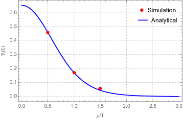
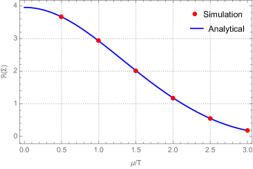
All in all, we were able to compute almost everything in a wide region of the parameter space covering a range of values for $N_{f}$, $m$ and $\mu/T$. Almost means that at high values of $N_{f}$, flat Monte Carlo simulations were successful at all values of $\mu/T$ (this is consistent with the observation that the model is easy to simulate at high $N_{f}$; in those regions the problem is isotropic and semiclassical estimates essentially become exact in the limit $N_{f}\rightarrow\infty$). On the other side, for other values of parameters (namely, large $\mu/T$ at small $N_{f}$) results could not be calculated (see Figure 1).

(a) $m=0.1$, $N_{f}=1$

(b) $m=0.1$, $N_{f}=12$

Figure 1: Situation one year ago: (right) chiral condensate correctly computed for high $N_{f}$ (here $N_{f}=12$); (left) for $N_{f}=1$ we could not get results beyond a given value of $\mu/T$.

4 Improving on previous results

4.1 Reflection symmetry

Simmetries always play an important role: not surprisingly, we have a symmetry at hand which lets us check our results and which also makes our life easier Tanizaki:2015pua . The QCD action (in our case, we only have the Dirac determinant) is invariant under charge conjugation $\mathcal{C}$ defined by

$$\mathcal{C}\begin{cases}\psi\rightarrow C^{-1}\bar{\psi}^{T}\\ \bar{\psi}\rightarrow-\psi^{T}C\\ U_{\hat{\nu}}(n)\rightarrow\bar{U}_{\hat{\nu}}(n)&\left(A_{\hat{\nu}}(n)\rightarrow-A^{T}_{\hat{\nu}}(n)=-\bar{A}\right)\\ \mu\rightarrow-\mu\end{cases}$$

Together with the generalization of $\gamma_{5}$-hermiticity at finite chemical potential

$$\det D(U,-\mu)=\overline{\det D(U,\mu)}$$

this implies that

$$\overline{S(A)}\sim\overline{\det D(U,\mu)}\overset{\gamma_{5}\text{-herm.}}{=}\det D(U,-\mu)\overset{\mathcal{C}\text{-inv.}}{=}\det D(\bar{U},\mu)\sim S(-\bar{A})$$

We thus expect thimbles to appear in conjugate pairs. Consider the $\{U_{k}\}$. $U_{0}={\mathbb{1}}$ is real and therefore self-conjugate (i.e. computations on the associated thimble yield real results). Being $e^{4\pi i/3}=e^{-2\pi i/3}$, we immediately see that $U_{2}=\overline{U_{1}}$: $U_{1}$ and $U_{2}$ are a conjugate pair of critical points and results of integration on $U_{2}$ should be the complex conjugate of those on $U_{1}$, yielding an overall real contribution to the partition function and to the expectation value of observables as well. All this is well evident in numerical simulations and in all the numerical results that we present in the following we take advantage of this symmetry: the real part of results from thimble 1 and 2 have been averaged.

4.2 Importance sampling

If a single thimble contributed, the computation of (1) would simply amount to

$$\langle O\rangle={{\langle O\,e^{i\,\omega}\rangle_{\sigma}}\over{\langle e^{i\,\omega}\rangle_{\sigma}}}\;\;\;\;\;\;\;\;\;\mbox{with}\;\;\;\;\;\;\;\;\;\langle\ldots\rangle_{\sigma}={{\int\limits_{\mathcal{J}_{\sigma}}\mathrm{d}^{n}y\,\ldots\,e^{-S_{R}}}\over{\int\limits_{\mathcal{J}_{\sigma}}\mathrm{d}^{n}y\,e^{-S_{R}}}}$$ (6)

In terms of the representation (2), we can now rephrase

$$\langle f\rangle_{\sigma}={{1}\over{Z_{\sigma}}}\int\limits_{\mathcal{J}_{\sigma}}\mathrm{d}^{n}y\,f\,e^{-S_{R}}={{1}\over{Z_{\sigma}}}\int\mathrm{D}\hat{n}\;(2\sum_{i=1}^{n}\lambda_{i}n_{i}^{2})\int\limits_{-\infty}^{+\infty}\mathrm{d}t\,f(\hat{n},t)\,e^{-S_{\mathrm{eff}}(\hat{n},t)}=\int\mathrm{D}\hat{n}\,{{Z_{\hat{n}}}\over{Z_{\sigma}}}\,f_{\hat{n}}$$ (7)

where

$$f_{\hat{n}}\equiv{{1}\over{Z_{\hat{n}}}}(2\sum_{i=1}^{n}\lambda_{i}n_{i}^{2})\int\limits_{-\infty}^{+\infty}\mathrm{d}t\,f(\hat{n},t)\,e^{-S_{\mathrm{eff}}(\hat{n},t)}\;\;\;\;\;\;\;\;\;\mbox{and}\;\;\;\;\;\;\;\;\;Z_{\hat{n}}^{(\sigma)}=2\sum_{i=1}^{n}\lambda_{i}^{(\sigma)}n_{i}^{2}\int\limits_{-\infty}^{+\infty}\mathrm{d}t\,e^{-S_{\mathrm{eff}}^{(\sigma)}(\hat{n},t)}.$$

Now, $f_{\hat{n}}$ looks like a functional integral along a single complete flow line. On the other side, (7) is nothing but the average of the $f_{\hat{n}}$ (i.e. the average of the contributions that a given observable takes from complete flow lines) and the weight $Z_{\hat{n}}/Z_{\sigma}$ represents the fraction of the partition function which is provided by a single complete flow line. $Z_{\hat{n}}/Z_{\sigma}$ provides a natural setting for importance sampling: directions $\hat{n}$ have to be extracted according to the probability $P(\hat{n})=Z_{\hat{n}}/Z_{\sigma}$.

We thus proceed as follow. Sitting on the current configuration (associated to a direction $\hat{n}$), we propose a new one (associated to a direction $\hat{n}^{\prime}$). $\hat{n}^{\prime}$ is identical to $\hat{n}$ apart from two randomly chosen components, say $(n_{i},n_{j})$ with $i\neq j$. Given the normalization $\left|\vec{n}\right|=\sqrt{\mathcal{R}}$ and the values of all $\{n_{k}\}_{k\neq i,j}$ we define $C$ as

$$C\equiv n_{i}^{2}+n_{j}^{2}=\mathcal{R}-\sum_{k\neq i,j}n_{k}^{2}$$

and we observe that there is a coordinate system in which the current values of $(n_{i},n_{j})$ are parametrized as

$$n_{i}=\sqrt{C}\,\cos\phi\;\;\;\;\;n_{j}=\sqrt{C}\,\sin\phi$$

with $\phi\in[0,2\pi)$. Now we change $\phi\rightarrow\phi^{\prime}$ by extracting $\phi^{\prime}-\phi$ flat in a given (tunable) range. This results in $(n_{i},n_{j})\rightarrow(n_{i}^{\prime},n_{j}^{\prime})$, while for all the other components (${k\neq i,j}$) $n_{k}=n_{k}^{\prime}$. We finally accept the proposed configuration with the standard Metropolis test

$$P_{\mathrm{acc}}\left(\hat{n}^{\prime}\bigr{|}\hat{n}\right)=\min\left\{1,{{Z_{\hat{n}^{\prime}}}\over{Z_{\hat{n}}}}\right\}.$$ (8)

In our case three contributions should be in principle taken into account. Actually, due to the symmetry of Section 4.1, only two distinct contributions are in place and we have to compute

$$\langle O\rangle={{n_{0}\,e^{-i\,S_{I0}}\,Z_{0}\,\langle O\,e^{i\,\omega}\rangle_{0}\,+\,n_{12}\,e^{-i\,S_{I12}}\,Z_{12}\,\langle O\,e^{i\,\omega}\rangle_{12}}\over{n_{0}\,e^{-i\,S_{I0}}\,Z_{0}\,\langle e^{i\,\omega}\rangle_{0}\,+\,n_{12}\,e^{-i\,S_{I12}}\,Z_{12}\,\langle e^{i\,\omega}\rangle_{12}}}$$ (9)

in which subscript notations should be evident. In DiRenzo:2015foa we observed that equation (9) can be rewritten

$$\langle O\rangle={{\langle O\,e^{i\,\omega}\rangle_{0}\,+\,\alpha\langle O\,e^{i\,\omega}\rangle_{12}}\over{\langle e^{i\,\omega}\rangle_{0}\,+\,\alpha\langle e^{i\,\omega}\rangle_{12}}}$$ (10)

where we defined

$$\alpha\equiv{{n_{12}\,e^{-i\,S_{I12}}\,Z_{12}}\over{n_{0}\,e^{-i\,S_{I0}}\,Z_{0}}}$$ (11)

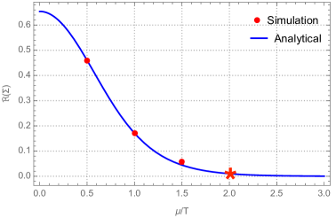
The idea is now to take a given observable as a normalization point, thus determining the value of $\alpha$. All the other observables of the theory can then be computed using this input. This could indeed be successfully done. Figure 2 confirms the effectiveness of the procedure. For $N_{f}=1,m=0.1$ the point $\mu/T=2.0$ was completely out of reach for flat, crude Monte Carlo, while results are successfully computed with the improved method. At these values of parameters the tiny value of the chiral condensate (of order $10^{-2}$) results from a delicate cancelation of the contributions coming from the different thimbles. This has nothing to do with the original sign problem (nor e.g. with the residual phase), but it is simply a numerical accident occurring for a given observable at a given value of parameters.

(a) $m=0.1$, $N_{f}=1$

(b) $m=0.1$, $N_{f}=1$ (new!)

Figure 2: An example of succesfull improvement: (left) as in Figure 1; (right) a new point computed via the improved method.

5 Conclusions

There is still quite a long way to go before thimble regularization can tackle the real goal, i.e. QCD at finite density. This work nevertheless shows that simulations on multiple thimbles are viable.

References

- (1) M. Cristoforetti, F. Di Renzo, L. Scorzato, Phys. Rev. D86, 074506 (2012), 1205.3996
- (2) H. Fujii, D. Honda, M. Kato, Y. Kikukawa, S. Komatsu, T. Sano, JHEP 1310, 147 (2013), 1309.4371
- (3) M. Cristoforetti, F. Di Renzo, G. Eruzzi, A. Mukherjee, C. Schmidt, L. Scorzato, C. Torrero, Phys. Rev. D89, 114505 (2014), 1403.5637
- (4) A. Alexandru, G. Basar, P. Bedaque, G. Ridgway, N. Warrington, JHEP 1605, 053 (2016), 1512.08764
- (5) H. Fujii, s. Kamata, Y. Kikukawa, JHEP 1512, 172 (2015), [Erratum: JHEP02,036(2016)], 1509.09141
- (6) Y. Tanizaki, Y. Hidaka, T. Hayata, New J. Phys. 18, 033002 (2016), 1509.07146
- (7) F. Di Renzo, G. Eruzzi, PoS LATTICE 2016, 047 (2016), 1611.08223
- (8) F. Di Renzo, G. Eruzzi, Phys. Rev. D92, 085030 (2015), 1507.03858
- (9) J. Bloch, F. Bruckmann, T. Wettig, JHEP 1310, 140 (2013), 1307.1416
- (10) F. Di Renzo, G. Eruzzi (2017), 1709:10468
- (11) Y. Tanizaki, H. Nishimura, K. Kashiwa, Phys. Rev. D91, 101701 (2015), 1504.02979