Heterogeneity and strong competition in ecology

Harsha Hutridurga H.H.: Department of Mathematics, Imperial College London, London, SW7 2AZ, United Kingdom. h.hutridurga-ramaiah@imperial.ac.uk  and  Chandrasekhar Venkataraman C.V.: School of Mathematics and Statistics, North Haugh, St Andrews KY16 9SS, United Kingdom. cv28@st-andrews.ac.uk
Abstract.

We study a competition-diffusion model while performing simultaneous homogenization and strong competition limits. The limit problem is shown to be a Stefan type evolution equation with effective coefficients. We also perform some numerical simulations in one and two spatial dimensions that suggest that oscillations are detrimental to invasion behaviour of the species.

Keywords: Homogenization, Equations in media with periodic structures, Asymptotic analysis, Stefan problems, Finite element methods, Ecology and invasion.

1. Introduction

This article attempts to understand the effect of rapid oscillations in the diffusion coefficients in strong competition limits of models from theoretical ecology. In particular, the current work provides a starting point towards understanding the role played by heterogeneous mobility on invasion behaviour in models for competition between two motile species. For analytical tractability, we consider only periodic oscillations in the diffusivities. Take Y:=[0,1)dassign𝑌superscript01𝑑Y:=[0,1)^{d} to be the unit reference periodicity cell. Consider bounded positive definite matrices A,BL(Y;d×d)𝐴𝐵superscriptL𝑌superscript𝑑𝑑A,B\in\mathrm{L}^{\infty}(Y;{\mathbb{R}}^{d\times d}), i.e., there exists a positive constant β𝛽\beta such that

ζA(y)ζβ|ζ|2,ζB(y)ζβ|ζ|2 for a.e. yY and ζd,formulae-sequencesuperscript𝜁top𝐴𝑦𝜁𝛽superscript𝜁2formulae-sequencesuperscript𝜁top𝐵𝑦𝜁𝛽superscript𝜁2 for a.e. 𝑦𝑌 and for-all𝜁superscript𝑑\displaystyle\zeta^{\top}\!\!A(y)\zeta\geq\beta\left|\zeta\right|^{2},\qquad\zeta^{\top}\!\!B(y)\zeta\geq\beta\left|\zeta\right|^{2}\quad\mbox{ for a.e. }y\in Y\mbox{ and }\forall\zeta\in{\mathbb{R}}^{d},

where we use superscripttop\cdot^{\top} to denote the transpose. As is classical in the periodic homogenization setting, we extend A𝐴A and B𝐵B to the full-space by Y𝑌Y-periodicity, i.e.,

A(x)=A(x+k𝐞i)B(x)=B(x+k𝐞i) for a.e. xd and kdi{1,,d},formulae-sequence𝐴𝑥𝐴𝑥𝑘subscript𝐞𝑖missing-subexpression𝐵𝑥𝐵𝑥𝑘subscript𝐞𝑖missing-subexpression for a.e. 𝑥superscript𝑑 and for-all𝑘superscript𝑑for-all𝑖1𝑑\begin{array}[]{cc}A(x)=A(x+k\,{\bf e}_{i})\\[5.69046pt] B(x)=B(x+k\,{\bf e}_{i})\end{array}\quad\mbox{ for a.e. }x\in{\mathbb{R}}^{d}\mbox{ and }\forall k\in\mathbb{Z}^{d}\quad\forall i\in\{1,\cdots,d\},

with {𝐞i}i=1dsuperscriptsubscriptsubscript𝐞𝑖𝑖1𝑑\{{\bf e}_{i}\}_{i=1}^{d} denoting the canonical basis in dsuperscript𝑑{\mathbb{R}}^{d}. Taking 0<ε10𝜀much-less-than10<\varepsilon\ll 1 to be the heterogeneity length scale, we define highly oscillating diffusion coefficients as

Aε(x):=A(xε);Bε(x):=B(xε) for xΩ.formulae-sequenceassignsuperscript𝐴𝜀𝑥𝐴𝑥𝜀formulae-sequenceassignsuperscript𝐵𝜀𝑥𝐵𝑥𝜀 for 𝑥Ω\displaystyle A^{\varepsilon}(x):=A\left(\frac{x}{\varepsilon}\right);\qquad B^{\varepsilon}(x):=B\left(\frac{x}{\varepsilon}\right)\qquad\mbox{ for }x\in\Omega.

Note that smaller the parameter ε𝜀\varepsilon is, greater will be the oscillations in Aεsuperscript𝐴𝜀A^{\varepsilon} and Bεsuperscript𝐵𝜀B^{\varepsilon} defined above. We would like to understand the dynamics of competition-diffusion in the context of two populations, say 𝒮1subscript𝒮1\mathcal{S}_{1} and 𝒮2subscript𝒮2\mathcal{S}_{2}, whose respective population densities are denoted as uε(t,x),vε(t,x)superscript𝑢𝜀𝑡𝑥superscript𝑣𝜀𝑡𝑥u^{\varepsilon}(t,x),v^{\varepsilon}(t,x). Note that the integral

uε(t,x)dxsubscriptsuperscript𝑢𝜀𝑡𝑥differential-d𝑥\displaystyle\int\limits_{\mathcal{B}}u^{\varepsilon}(t,x)\,{\rm d}x

represents the number of 𝒮1subscript𝒮1\mathcal{S}_{1} individuals in a region ΩΩ\mathcal{B}\subset\Omega at any given instant t>0𝑡0t>0. Similar interpretation holds for the population density vε(t,x)superscript𝑣𝜀𝑡𝑥v^{\varepsilon}(t,x). For the above two population densities and for a non-negative function wε(t,x)superscript𝑤𝜀𝑡𝑥w^{\varepsilon}(t,x), we consider a competition-diffusion system with heterogeneous diffusivities

(1) tuε(Aε(x)uε)+uεε(vε+λ(1wε))subscript𝑡superscript𝑢𝜀superscript𝐴𝜀𝑥superscript𝑢𝜀superscript𝑢𝜀𝜀superscript𝑣𝜀𝜆1superscript𝑤𝜀\displaystyle\partial_{t}u^{\varepsilon}-\nabla\cdot\Big{(}A^{\varepsilon}(x)\nabla u^{\varepsilon}\Big{)}+\frac{u^{\varepsilon}}{\varepsilon}\Big{(}v^{\varepsilon}+\lambda\left(1-w^{\varepsilon}\right)\Big{)} =0absent0\displaystyle=0 in (0,)×Ω,in 0Ω\displaystyle\mbox{ in }(0,\ell)\times\Omega,
tvε(Bε(x)vε)+αvεε(uε+λwε)subscript𝑡superscript𝑣𝜀superscript𝐵𝜀𝑥superscript𝑣𝜀𝛼superscript𝑣𝜀𝜀superscript𝑢𝜀𝜆superscript𝑤𝜀\displaystyle\partial_{t}v^{\varepsilon}-\nabla\cdot\Big{(}B^{\varepsilon}(x)\nabla v^{\varepsilon}\Big{)}+\alpha\frac{v^{\varepsilon}}{\varepsilon}\Big{(}u^{\varepsilon}+\lambda w^{\varepsilon}\Big{)} =0absent0\displaystyle=0 in (0,)×Ω,in 0Ω\displaystyle\mbox{ in }(0,\ell)\times\Omega,
twε+uεε(wε1)+wεvεεsubscript𝑡superscript𝑤𝜀superscript𝑢𝜀𝜀superscript𝑤𝜀1superscript𝑤𝜀superscript𝑣𝜀𝜀\displaystyle\partial_{t}w^{\varepsilon}+\frac{u^{\varepsilon}}{\varepsilon}\left(w^{\varepsilon}-1\right)+\frac{w^{\varepsilon}v^{\varepsilon}}{\varepsilon} =0absent0\displaystyle=0 in (0,)×Ω.in 0Ω\displaystyle\mbox{ in }(0,\ell)\times\Omega.

The interspecific competition rates between uεsuperscript𝑢𝜀u^{\varepsilon} and vεsuperscript𝑣𝜀v^{\varepsilon} in the above evolution is of 𝒪(ε1)𝒪superscript𝜀1\mathcal{O}(\varepsilon^{-1}). Here the positive parameter α𝛼\alpha governs the relative competitive strength of the two species, if α>1𝛼1\alpha>1, 𝒮1subscript𝒮1\mathcal{S}_{1} has a competitive advantage over 𝒮2subscript𝒮2\mathcal{S}_{2} whilst if α<1𝛼1\alpha<1, 𝒮2subscript𝒮2\mathcal{S}_{2} has a competitive advantage over 𝒮1subscript𝒮1\mathcal{S}_{1}. The unknown wε(t,x)superscript𝑤𝜀𝑡𝑥w^{\varepsilon}(t,x) may be thought of as an approximation of the characteristic function of the population density for the species 𝒮1subscript𝒮1\mathcal{S}_{1}, similarly (1wε(t,x))1superscript𝑤𝜀𝑡𝑥(1-w^{\varepsilon}(t,x)) may be thought of as an approximation of the characteristic function of the population density for the species 𝒮2subscript𝒮2\mathcal{S}_{2}. This interpretation allows an ecological interpretation of the reaction terms involving wε(t,x)superscript𝑤𝜀𝑡𝑥w^{\varepsilon}(t,x) as representing the cost to a species of converting the habitat of the other species into its own habitat [HIMN01]. The parameter λ0𝜆0\lambda\geq 0 governs the relative strength of this cost to direct interspecies competition effects, and we note that our results remain valid in the case λ=0𝜆0\lambda=0 which corresponds to no cost of habitat conversion. The evolution system (1) for (uε,vε,wε)superscript𝑢𝜀superscript𝑣𝜀superscript𝑤𝜀(u^{\varepsilon},v^{\varepsilon},w^{\varepsilon}) is supplemented by initial and boundary conditions

(2) uε(0,x)=uin(x),vε(0,x)=vin(x),wε(0,x)formulae-sequencesuperscript𝑢𝜀0𝑥superscript𝑢in𝑥superscript𝑣𝜀0𝑥superscript𝑣in𝑥superscript𝑤𝜀0𝑥\displaystyle u^{\varepsilon}(0,x)=u^{\rm in}(x),\,v^{\varepsilon}(0,x)=v^{\rm in}(x),\,w^{\varepsilon}(0,x) =win(x)absentsuperscript𝑤in𝑥\displaystyle=w^{\rm in}(x) in Ωin Ω\displaystyle\mbox{ in }\Omega
Aε(x)uε𝐧(x)=Bε(x)vε𝐧(x)superscript𝐴𝜀𝑥superscript𝑢𝜀𝐧𝑥superscript𝐵𝜀𝑥superscript𝑣𝜀𝐧𝑥\displaystyle A^{\varepsilon}(x)\nabla u^{\varepsilon}\cdot{\bf n}(x)=B^{\varepsilon}(x)\nabla v^{\varepsilon}\cdot{\bf n}(x) =0absent0\displaystyle=0 on (0,)×Ω.on 0Ω\displaystyle\mbox{ on }(0,\ell)\times\partial\Omega.

Here 𝐧(x)𝐧𝑥{\bf n}(x) is the unit exterior normal to ΩΩ\Omega at xΩ𝑥Ωx\in\partial\Omega. The initial data are assumed to be non-negative and bounded in LsuperscriptL\mathrm{L}^{\infty}, i.e.,

(3) 0uinumax<,0vinvmax<,0win1.formulae-sequence0superscript𝑢insubscript𝑢max0superscript𝑣insubscript𝑣max0superscript𝑤in1\displaystyle 0\leq u^{\rm in}\leq u_{\rm max}<\infty,\quad 0\leq v^{\rm in}\leq v_{\rm max}<\infty,\quad 0\leq w^{\rm in}\leq 1.

The competition-diffusion model (1)-(2) is essentially the evolution model considered in [HIMN01] except for the high frequency oscillations in the diffusion coefficients.
The present work deals with the asymptotic analysis of the coupled system (1)-(2) in the ε0𝜀0\varepsilon\to 0 limit and in the t1much-greater-than𝑡1t\gg 1 regime. The ε0𝜀0\varepsilon\to 0 limit procedure corresponds to performing both the homogenization and the strong competition limit simultaneously. The study of strong competition limits for such systems with constant diffusivities are found in [DHMP99, HIMN01]. The novelty of this work is to consider the effect of having highly oscillating diffusivities on the strong competition limit. We employ the method of two-scale convergence to address the periodic homogenization problem. Our main result is Theorem 13 which says that the solution family (uε,vε,wε)superscript𝑢𝜀superscript𝑣𝜀superscript𝑤𝜀(u^{\varepsilon},v^{\varepsilon},w^{\varepsilon}) to (1)-(2) has a limit point (u,v,w)superscript𝑢superscript𝑣superscript𝑤(u^{\ast},v^{\ast},w^{\ast}) in certain weak topology. The theorem further characterises the limit point as a solution to a certain Stefan type problem. The study of the long time behaviour of such models is treated numerically where we have performed numerical simulations to make some interesting observations on the so-called competitive Lotka-Volterra system in theoretical ecology.

The organization of this paper is as follows. In section 2, we briefly recall the existence and uniqueness theory for the competition-diffusion model (1)-(2) and gather some quantitative estimates on the solution family. Section 3 deals with our main result and its proof. The definition of two-scale convergence and associated compactness results are recalled in section 3. Our numerical results with emphasis on theoretical ecology are given in section 4. Eventually, section 5 proposes a more general setting where we consider multiple scales in the competition-diffusion systems. Some interesting observations from the periodic homogenization theory are gathered in Appendix A.

Acknowledgement: The research of the first author was supported by the EPSRC programme grant “Mathematical fundamentals of Metamaterials for multiscale Physics and Mechanic” (EP/L024926/1). The second author would like to thank the Isaac Newton Institute for Mathematical Sciences for support and hospitality during the program “Coupling geometric PDEs with physics for cell morphology, motility and pattern formation” where this project was initiated. Authors further thank the kind hospitality of the Hausdorff Institute for Mathematics in Bonn during the trimester program on multiscale problems in 2017 where some of this work was in progress. The authors would like to thank Henrik Shahgholian for his fruitful suggestions during the preparation of this article.

2. Existence analysis and preliminary estimates

The well-posedness of the initial boundary value problem (1)-(2) is a bit subtle. We cannot straightaway deduce the existence and uniqueness of solutions from the existence theory of reaction-diffusion systems. The reason being the absence of diffusion for wε(t,x)superscript𝑤𝜀𝑡𝑥w^{\varepsilon}(t,x) in the evolution (1). We borrow the associated well-posedness result from [HIMN01, Lemma 2.2, page 167] (see [HIMN01, section 5, pp. 178–180] for a sketch of proof).

Proposition 1.

Suppose the initial data satisfy (3). There exists a positive time >00\ell>0 such that, for each ε>0𝜀0\varepsilon>0, the competition-diffusion system (1)-(2) possesses a unique classical solution (uε,vε,wε)superscript𝑢𝜀superscript𝑣𝜀superscript𝑤𝜀(u^{\varepsilon},v^{\varepsilon},w^{\varepsilon}) in (0,)×Ω0Ω(0,\ell)\times\Omega.

Remark 2.

The result as stated in [HIMN01] does not speak about the global-in-time existence of solutions to the competition diffusion model. The proof of existence-uniqueness in [HIMN01] uses the contraction mapping principle. In this approach, they choose a final time \ell – see [HIMN01, page 180].
Even though there is no mention (in [HIMN01]) of extending the interval of existence in time to (0,)0(0,\infty), we could argue as in reaction-diffusion theories [Pie10, Lemma 1.1, page 420]. For example, as we have uniform (in time) LsuperscriptL\mathrm{L}^{\infty} bounds on the solution (uε,vε,wε)superscript𝑢𝜀superscript𝑣𝜀superscript𝑤𝜀(u^{\varepsilon},v^{\varepsilon},w^{\varepsilon}) – see Lemma 4, we can deduce global-in-time existence as there is no possibility of blow-up in LsuperscriptL\mathrm{L}^{\infty}-norm.

Next, we record a result on a conserved quantity for the competition-diffusion model (1)-(2).

Lemma 3.

Suppose the initial data satisfy (3). Then for each t(0,)𝑡0t\in(0,\infty), we have

Ω(uεvεα+λwε)(t,x)dx=Ω(uinvinα+λwin)(x)dxsubscriptΩsuperscript𝑢𝜀superscript𝑣𝜀𝛼𝜆superscript𝑤𝜀𝑡𝑥differential-d𝑥subscriptΩsuperscript𝑢insuperscript𝑣in𝛼𝜆superscript𝑤in𝑥differential-d𝑥\displaystyle\int\limits_{\Omega}\left(u^{\varepsilon}-\frac{v^{\varepsilon}}{\alpha}+\lambda w^{\varepsilon}\right)(t,x)\,{\rm d}x=\int\limits_{\Omega}\left(u^{\rm in}-\frac{v^{\rm in}}{\alpha}+\lambda w^{\rm in}\right)(x)\,{\rm d}x

for each ε>0𝜀0\varepsilon>0.

Proof.

Note that from the competition-diffusion system (1), we have

t(uεvεα+λwε)=(Aε(x)uε)(Bε(x)vε).subscript𝑡superscript𝑢𝜀superscript𝑣𝜀𝛼𝜆superscript𝑤𝜀superscript𝐴𝜀𝑥superscript𝑢𝜀superscript𝐵𝜀𝑥superscript𝑣𝜀\displaystyle\partial_{t}\left(u^{\varepsilon}-\frac{v^{\varepsilon}}{\alpha}+\lambda w^{\varepsilon}\right)=\nabla\cdot\Big{(}A^{\varepsilon}(x)\nabla u^{\varepsilon}\Big{)}-\nabla\cdot\Big{(}B^{\varepsilon}(x)\nabla v^{\varepsilon}\Big{)}.

Integrating the above equality over ΩΩ\Omega and employing the zero-flux boundary conditions from (2), we arrive at

ddtΩ(uεvεα+λwε)(t,x)dx=0dd𝑡subscriptΩsuperscript𝑢𝜀superscript𝑣𝜀𝛼𝜆superscript𝑤𝜀𝑡𝑥differential-d𝑥0\displaystyle\frac{{\rm d}}{{\rm d}t}\int\limits_{\Omega}\left(u^{\varepsilon}-\frac{v^{\varepsilon}}{\alpha}+\lambda w^{\varepsilon}\right)(t,x)\,{\rm d}x=0

which when integrated in the time variable yields the result. ∎

We record a result, thanks to the Maximum principle (see [HIMN01, Lemma 2.3, page 168]).

Lemma 4.

Suppose the initial data satisfy (3). Then the solution (uε,vε,wε)superscript𝑢𝜀superscript𝑣𝜀superscript𝑤𝜀(u^{\varepsilon},v^{\varepsilon},w^{\varepsilon}) to the competition-diffusion model (1)-(2) satisfies

0uε(t,x)umax,0vε(t,x)vmax,0wε(t,x)1formulae-sequence0superscript𝑢𝜀𝑡𝑥subscript𝑢max0superscript𝑣𝜀𝑡𝑥subscript𝑣max0superscript𝑤𝜀𝑡𝑥1\displaystyle 0\leq u^{\varepsilon}(t,x)\leq u_{\rm max},\quad 0\leq v^{\varepsilon}(t,x)\leq v_{\rm max},\quad 0\leq w^{\varepsilon}(t,x)\leq 1

for each ε>0𝜀0\varepsilon>0 and for all (t,x)(0,)×Ω𝑡𝑥0Ω(t,x)\in(0,\ell)\times\Omega.

The following result gives a priori bounds on the solutions to (1) via energy method (see [HIMN01, Lemma 2.4, pp.  168–169] for proof).

Proposition 5 (a priori estimates).

Suppose the initial data satisfy (3). Let (uε,vε,wε)superscript𝑢𝜀superscript𝑣𝜀superscript𝑤𝜀(u^{\varepsilon},v^{\varepsilon},w^{\varepsilon}) be the solution to the competition model (1). Then we have

(4) uεL2((0,)×Ω)C;vεL2((0,)×Ω)C;formulae-sequencesubscriptnormsuperscript𝑢𝜀superscriptL20Ω𝐶subscriptnormsuperscript𝑣𝜀superscriptL20Ω𝐶\displaystyle\left\|\nabla u^{\varepsilon}\right\|_{\mathrm{L}^{2}((0,\ell)\times\Omega)}\leq C;\qquad\left\|\nabla v^{\varepsilon}\right\|_{\mathrm{L}^{2}((0,\ell)\times\Omega)}\leq C;
(5) uεvεL1((0,)×Ω)Cε;uε(1wε)L1((0,)×Ω)Cε;formulae-sequencesubscriptnormsuperscript𝑢𝜀superscript𝑣𝜀superscriptL10Ω𝐶𝜀subscriptnormsuperscript𝑢𝜀1superscript𝑤𝜀superscriptL10Ω𝐶𝜀\displaystyle\left\|u^{\varepsilon}v^{\varepsilon}\right\|_{\mathrm{L}^{1}((0,\ell)\times\Omega)}\leq C\varepsilon;\qquad\left\|u^{\varepsilon}\left(1-w^{\varepsilon}\right)\right\|_{\mathrm{L}^{1}((0,\ell)\times\Omega)}\leq C\varepsilon;
vεwεL1((0,)×Ω)Cε.subscriptnormsuperscript𝑣𝜀superscript𝑤𝜀superscriptL10Ω𝐶𝜀\displaystyle\left\|v^{\varepsilon}w^{\varepsilon}\right\|_{\mathrm{L}^{1}((0,\ell)\times\Omega)}\leq C\varepsilon.

As the impending asymptotic analysis needs to address the nonlinearities in our model, it is essential to obtain strong compactness of our solution family. To that end, we record the following estimates on the time translates (see [HIMN01, Lemma 2.5, pp.  169–171] for proof).

Lemma 6.

Let (uε,vε,wε)superscript𝑢𝜀superscript𝑣𝜀superscript𝑤𝜀(u^{\varepsilon},v^{\varepsilon},w^{\varepsilon}) be the solution to the competition model (1). Then for τ>0𝜏0\tau>0,

(6) 0τΩ|uε(t+τ,x)uε(t,x)|2dxdtCτsuperscriptsubscript0𝜏subscriptΩsuperscriptsuperscript𝑢𝜀𝑡𝜏𝑥superscript𝑢𝜀𝑡𝑥2differential-d𝑥differential-d𝑡𝐶𝜏\displaystyle\int\limits_{0}^{\ell-\tau}\int\limits_{\Omega}\left|u^{\varepsilon}(t+\tau,x)-u^{\varepsilon}(t,x)\right|^{2}\,{\rm d}x\,{\rm d}t\leq C\tau
0τΩ|vε(t+τ,x)vε(t,x)|2dxdtCτ.superscriptsubscript0𝜏subscriptΩsuperscriptsuperscript𝑣𝜀𝑡𝜏𝑥superscript𝑣𝜀𝑡𝑥2differential-d𝑥differential-d𝑡𝐶𝜏\displaystyle\int\limits_{0}^{\ell-\tau}\int\limits_{\Omega}\left|v^{\varepsilon}(t+\tau,x)-v^{\varepsilon}(t,x)\right|^{2}\,{\rm d}x\,{\rm d}t\leq C\tau.

Note that the family of population densities uεsuperscript𝑢𝜀u^{\varepsilon} and vεsuperscript𝑣𝜀v^{\varepsilon} are uniformly bounded in L2((0,)×Ω)superscriptL20Ω\mathrm{L}^{2}((0,\ell)\times\Omega), i.e.,

uεL2((0,)×Ω)C;vεL2((0,)×Ω)Cformulae-sequencesubscriptnormsuperscript𝑢𝜀superscriptL20Ω𝐶subscriptnormsuperscript𝑣𝜀superscriptL20Ω𝐶\displaystyle\left\|u^{\varepsilon}\right\|_{\mathrm{L}^{2}((0,\ell)\times\Omega)}\leq C;\qquad\left\|v^{\varepsilon}\right\|_{\mathrm{L}^{2}((0,\ell)\times\Omega)}\leq C

with the positive constant C𝐶C being independent of ε𝜀\varepsilon, thanks to the uniform LsuperscriptL\mathrm{L}^{\infty} estimates from Lemma 4. Combining this with the estimate (4) yields a uniform estimate in L2((0,);H1(Ω))superscriptL20superscriptH1Ω\mathrm{L}^{2}((0,\ell);\mathrm{H}^{1}(\Omega)). Note further that Lemma 6 gives the L2superscriptL2\mathrm{L}^{2} estimates on the time translates of the families uεsuperscript𝑢𝜀u^{\varepsilon} and vεsuperscript𝑣𝜀v^{\varepsilon}. Hence we can invoke the Aubin-Lions compactness criterion to arrive at the following relative compactness result on the families of the population densities.

Proposition 7 (Relative compactness).

Let uε(t,x)superscript𝑢𝜀𝑡𝑥u^{\varepsilon}(t,x) and vε(t,x)superscript𝑣𝜀𝑡𝑥v^{\varepsilon}(t,x) be the family of population densities associated with the evolution system (1)-(2). Then, up to extraction of subsequence, we have

uεsuperscript𝑢𝜀\displaystyle u^{\varepsilon} ––→u strongly in L2((0,)×Ω),––→absentsuperscript𝑢 strongly in superscriptL20Ω\displaystyle\relbar\joinrel\relbar\joinrel\relbar\joinrel\relbar\joinrel\to u^{*}\mbox{ strongly in }\mathrm{L}^{2}((0,\ell)\times\Omega),
vεsuperscript𝑣𝜀\displaystyle v^{\varepsilon} ––→v strongly in L2((0,)×Ω).––→absentsuperscript𝑣 strongly in superscriptL20Ω\displaystyle\relbar\joinrel\relbar\joinrel\relbar\joinrel\relbar\joinrel\to v^{*}\mbox{ strongly in }\mathrm{L}^{2}((0,\ell)\times\Omega).
Remark 8.

The approach in [HIMN01] to obtain strong compactness of the family is to treat the translates in both the space time variables and employ the Kolmogorov-Riesz-Fréchet criterion in space-time [Bre10, Theorem 4.26, page 111]. One can also obtain the aforementioned compactness via the criterion mentioned in Simon’s seminal paper [Sim86, Theorem 1, page 71].

3. Two-scale convergence and homogenization

In this section, we briefly recall the notion of two-scale converegence introduced by Nguetseng [Ngu89] and further developed by Allaire [All92]. This is a notion of multi-scale weak convergence which captures oscillations in a function sequence. To be precise, let us recall the definition. As this paper deals with function sequences that depend on the time variable, we make the choice of presenting the two-scale convergence theory with the time variable. However, the time variable simply plays the role of a parameter. Furthermore, we only give the definition in the L2superscriptL2\mathrm{L}^{2}-setting. The theory of two-scale convergence is also available in LpsuperscriptL𝑝\mathrm{L}^{p}-spaces with p(1,)𝑝1p\in(1,\infty).

Definition 9 (Two-scale convergence).

A family fεL2((0,)×Ω)superscript𝑓𝜀superscriptL20Ωf^{\varepsilon}\subset\mathrm{L}^{2}((0,\ell)\times\Omega) is said to two-scale converge to a limit f0(t,x,y)L2((0,)×Ω×Y)subscript𝑓0𝑡𝑥𝑦superscriptL20Ω𝑌f_{0}(t,x,y)\in\mathrm{L}^{2}((0,\ell)\times\Omega\times Y) if the following limit holds for any smooth test function ψ(t,x,y)𝜓𝑡𝑥𝑦\psi(t,x,y) which is Y𝑌Y-periodic in the y𝑦y variable

limε0(0,)×Ωfε(t,x)ψ(t,x,xε)dxdt=(0,)×Ω×Yf0(t,x,y)ψ(t,x,y)dydxdt.subscript𝜀0subscriptdouble-integral0Ωsuperscript𝑓𝜀𝑡𝑥𝜓𝑡𝑥𝑥𝜀differential-d𝑥differential-d𝑡subscripttriple-integral0Ω𝑌subscript𝑓0𝑡𝑥𝑦𝜓𝑡𝑥𝑦differential-d𝑦differential-d𝑥differential-d𝑡\displaystyle\lim_{\varepsilon\to 0}\iint\limits_{(0,\ell)\times\Omega}f^{\varepsilon}(t,x)\psi\left(t,x,\frac{x}{\varepsilon}\right)\,{\rm d}x\,{\rm d}t=\iiint\limits_{(0,\ell)\times\Omega\times Y}f_{0}(t,x,y)\psi(t,x,y)\,{\rm d}y\,{\rm d}x\,{\rm d}t.

We denote the above convergence as fε––-⇀2scalef0superscript––-⇀2𝑠𝑐𝑎𝑙𝑒superscript𝑓𝜀subscript𝑓0f^{\varepsilon}\stackrel{{\scriptstyle 2-scale}}{{\relbar\joinrel\relbar\joinrel\relbar\joinrel\relbar\joinrel\relbar\joinrel\rightharpoonup}}f_{0}.

The following compactness result is the cornerstone of the two-scale convergence theory (see [Ngu89, Theorem 1, p.611] and [All92, Theorem 1.2, p.1485]).

Theorem 10 (Two-scale compactness).

Suppose fε(t,x)superscript𝑓𝜀𝑡𝑥f^{\varepsilon}(t,x) is a uniformly bounded family in L2((0,)×Ω)superscriptL20Ω\mathrm{L}^{2}((0,\ell)\times\Omega), i.e.,

fεL2((0,)×Ω)Csubscriptnormsuperscript𝑓𝜀superscriptL20Ω𝐶\displaystyle\left\|f^{\varepsilon}\right\|_{\mathrm{L}^{2}((0,\ell)\times\Omega)}\leq C

with the constant C>0𝐶0C>0 being independent of ε𝜀\varepsilon. Then we can extract a subsequence, still denoted fε(t,x)superscript𝑓𝜀𝑡𝑥f^{\varepsilon}(t,x), and there exists a limit f0(t,x,y)L2((0,)×Ω×Y)subscript𝑓0𝑡𝑥𝑦superscriptL20Ω𝑌f_{0}(t,x,y)\in\mathrm{L}^{2}((0,\ell)\times\Omega\times Y) such that

fε––-⇀2scalef0.superscript––-⇀2𝑠𝑐𝑎𝑙𝑒superscript𝑓𝜀subscript𝑓0\displaystyle f^{\varepsilon}\stackrel{{\scriptstyle 2-scale}}{{\relbar\joinrel\relbar\joinrel\relbar\joinrel\relbar\joinrel\relbar\joinrel\rightharpoonup}}f_{0}.

Another important result in the two-scale convergence theory which makes it a valuable tool in periodic homogenization is as follows.

Theorem 11 (Two-scale compactness in H1superscriptH1\mathrm{H}^{1}).

Suppose fε(t,x)superscript𝑓𝜀𝑡𝑥f^{\varepsilon}(t,x) be a uniformly bounded family in L2((0,);H1(Ω))superscriptL20superscriptH1Ω\mathrm{L}^{2}((0,\ell);\mathrm{H}^{1}(\Omega)), i.e.,

(0,)×Ω|fε(t,x)|2dxdt+(0,)×Ω|fε(t,x)|2dxdtCsubscriptdouble-integral0Ωsuperscriptsuperscript𝑓𝜀𝑡𝑥2differential-d𝑥differential-d𝑡subscriptdouble-integral0Ωsuperscriptsuperscript𝑓𝜀𝑡𝑥2differential-d𝑥differential-d𝑡𝐶\displaystyle\iint\limits_{(0,\ell)\times\Omega}\left|f^{\varepsilon}(t,x)\right|^{2}\,{\rm d}x\,{\rm d}t+\iint\limits_{(0,\ell)\times\Omega}\left|\nabla f^{\varepsilon}(t,x)\right|^{2}\,{\rm d}x\,{\rm d}t\leq C

with the constant C>0𝐶0C>0 being independent of ε𝜀\varepsilon. Then we can extract a subsequence, still denoted fε(t,x)superscript𝑓𝜀𝑡𝑥f^{\varepsilon}(t,x), and there exist limits f0(t,x)L2((0,);H1(Ω))subscript𝑓0𝑡𝑥superscriptL20superscriptH1Ωf_{0}(t,x)\in\mathrm{L}^{2}((0,\ell);\mathrm{H}^{1}(\Omega)), f1(t,x,y)L2((0,)×Ω;H#1(Y)/)subscript𝑓1𝑡𝑥𝑦superscriptL20ΩsubscriptsuperscriptH1#𝑌f_{1}(t,x,y)\in\mathrm{L}^{2}((0,\ell)\times\Omega;\mathrm{H}^{1}_{\#}(Y)/{\mathbb{R}}) such that

fεsuperscript𝑓𝜀\displaystyle f^{\varepsilon} ––⇀f0 weakly in L2((0,);H1(Ω))––⇀absentsubscript𝑓0 weakly in superscript𝐿20superscriptH1Ω\displaystyle\relbar\joinrel\relbar\joinrel\relbar\joinrel\relbar\joinrel\rightharpoonup f_{0}\mbox{ weakly in }L^{2}((0,\ell);\mathrm{H}^{1}(\Omega))
fεsuperscript𝑓𝜀\displaystyle\nabla f^{\varepsilon} ––-⇀2scalexf0+yf1superscript––-⇀2𝑠𝑐𝑎𝑙𝑒absentsubscript𝑥subscript𝑓0subscript𝑦subscript𝑓1\displaystyle\stackrel{{\scriptstyle 2-scale}}{{\relbar\joinrel\relbar\joinrel\relbar\joinrel\relbar\joinrel\relbar\joinrel\rightharpoonup}}\nabla_{x}f_{0}+\nabla_{y}f_{1}

Refer to [Ngu89, Theorem 3, p.618] and [All92, Proposition 1.14, p.1491] for the proof of the above result. In the statement of Theorem 11, we have used the standard notation for Y𝑌Y-periodic function space

H#1(Y):={f:d such that f is Y-periodic and fH1(Y)<}.assignsubscriptsuperscriptH1#𝑌conditional-set𝑓superscript𝑑 such that 𝑓 is 𝑌-periodic and subscriptnorm𝑓superscriptH1𝑌\mathrm{H}^{1}_{\#}(Y):=\Big{\{}f:\mathbb{R}^{d}\to{\mathbb{R}}\,\,\mbox{ such that }\,\,f\mbox{ is }Y\mbox{-periodic and }\left\|f\right\|_{\mathrm{H}^{1}(Y)}<\infty\Big{\}}.

The following result states that a norm convergence information on the family implies that the family two-scale converges to the same limit (see [LNW02, Theorem 5, p.42] for the proof).

Theorem 12 (Convergence in norm).

Suppose fε(t,x)superscript𝑓𝜀𝑡𝑥f^{\varepsilon}(t,x) is a family which strongly converges in L2((0,)×Ω)superscriptL20Ω\mathrm{L}^{2}((0,\ell)\times\Omega) to f0(t,x)subscript𝑓0𝑡𝑥f_{0}(t,x), i.e.,

limε0(0,)×Ω|fε(t,x)f0(t,x)|2dxdt=0subscript𝜀0subscriptdouble-integral0Ωsuperscriptsuperscript𝑓𝜀𝑡𝑥subscript𝑓0𝑡𝑥2differential-d𝑥differential-d𝑡0\displaystyle\lim_{\varepsilon\to 0}\iint\limits_{(0,\ell)\times\Omega}\left|f^{\varepsilon}(t,x)-f_{0}(t,x)\right|^{2}\,{\rm d}x\,{\rm d}t=0

then we have

fε––-⇀2scalef0superscript––-⇀2𝑠𝑐𝑎𝑙𝑒superscript𝑓𝜀subscript𝑓0\displaystyle f^{\varepsilon}\stackrel{{\scriptstyle 2-scale}}{{\relbar\joinrel\relbar\joinrel\relbar\joinrel\relbar\joinrel\relbar\joinrel\rightharpoonup}}f_{0}

3.1. Homogenization result

In this subsection, we state and prove our main result on the ε0𝜀0\varepsilon\to 0 limit for the competition-diffusion model. Our strategy of proof is to employ the notion of two-scale convergence detailed earlier.

Theorem 13 (Homogenization limit).

Let (uε,vε,wε)superscript𝑢𝜀superscript𝑣𝜀superscript𝑤𝜀(u^{\varepsilon},v^{\varepsilon},w^{\varepsilon}) be the solution to the competition-diffusion model (1)-(2). Then there exists a subsequence (uε,vε,wε)superscript𝑢𝜀superscript𝑣𝜀superscript𝑤𝜀(u^{\varepsilon},v^{\varepsilon},w^{\varepsilon}) and functions uL2((0,);H1(Ω))superscript𝑢superscriptL20superscriptH1Ωu^{*}\in\mathrm{L}^{2}((0,\ell);\mathrm{H}^{1}(\Omega)), u1L2((0,)×Ω;H#1(Y)/)subscript𝑢1superscriptL20ΩsubscriptsuperscriptH1#𝑌u_{1}\in\mathrm{L}^{2}((0,\ell)\times\Omega;\mathrm{H}^{1}_{\#}(Y)/{\mathbb{R}}), vL2((0,);H1(Ω))superscript𝑣superscriptL20superscriptH1Ωv^{*}\in\mathrm{L}^{2}((0,\ell);\mathrm{H}^{1}(\Omega)), v1L2((0,)×Ω;H#1(Y)/)subscript𝑣1superscriptL20ΩsubscriptsuperscriptH1#𝑌v_{1}\in\mathrm{L}^{2}((0,\ell)\times\Omega;\mathrm{H}^{1}_{\#}(Y)/{\mathbb{R}}), wL2((0,)×Ω)superscript𝑤superscriptL20Ωw^{*}\in\mathrm{L}^{2}((0,\ell)\times\Omega) such that

(7) uεsuperscript𝑢𝜀\displaystyle u^{\varepsilon} ––→u strongly in L2((0,)×Ω)––→absentsuperscript𝑢 strongly in superscriptL20Ω\displaystyle\relbar\joinrel\relbar\joinrel\relbar\joinrel\relbar\joinrel\to u^{*}\mbox{ strongly in }\mathrm{L}^{2}((0,\ell)\times\Omega)
uεsuperscript𝑢𝜀\displaystyle\nabla u^{\varepsilon} ––-⇀2scalexu+yu1superscript––-⇀2𝑠𝑐𝑎𝑙𝑒absentsubscript𝑥superscript𝑢subscript𝑦subscript𝑢1\displaystyle\stackrel{{\scriptstyle 2-scale}}{{\relbar\joinrel\relbar\joinrel\relbar\joinrel\relbar\joinrel\relbar\joinrel\rightharpoonup}}\nabla_{x}u^{*}+\nabla_{y}u_{1}
vεsuperscript𝑣𝜀\displaystyle v^{\varepsilon} ––→v strongly in L2((0,)×Ω)––→absentsuperscript𝑣 strongly in superscriptL20Ω\displaystyle\relbar\joinrel\relbar\joinrel\relbar\joinrel\relbar\joinrel\to v^{*}\mbox{ strongly in }\mathrm{L}^{2}((0,\ell)\times\Omega)
vεsuperscript𝑣𝜀\displaystyle\nabla v^{\varepsilon} ––-⇀2scalexv+yv1superscript––-⇀2𝑠𝑐𝑎𝑙𝑒absentsubscript𝑥superscript𝑣subscript𝑦subscript𝑣1\displaystyle\stackrel{{\scriptstyle 2-scale}}{{\relbar\joinrel\relbar\joinrel\relbar\joinrel\relbar\joinrel\relbar\joinrel\rightharpoonup}}\nabla_{x}v^{*}+\nabla_{y}v_{1}
wεsuperscript𝑤𝜀\displaystyle w^{\varepsilon} ––⇀w weakly in L2((0,)×Ω).––⇀absentsuperscript𝑤 weakly in superscriptL20Ω\displaystyle\relbar\joinrel\relbar\joinrel\relbar\joinrel\relbar\joinrel\rightharpoonup w^{*}\mbox{ weakly in }\mathrm{L}^{2}((0,\ell)\times\Omega).

Furthermore, we have that the functions (u1,v1)subscript𝑢1subscript𝑣1(u_{1},v_{1}) can be decomposed as

(8) u1(t,x,y)=i=1dωi(y)uxi(t,x);v1(t,x,y)=i=1dχi(y)vxi(t,x)formulae-sequencesubscript𝑢1𝑡𝑥𝑦superscriptsubscript𝑖1𝑑subscript𝜔𝑖𝑦superscript𝑢subscript𝑥𝑖𝑡𝑥subscript𝑣1𝑡𝑥𝑦superscriptsubscript𝑖1𝑑subscript𝜒𝑖𝑦superscript𝑣subscript𝑥𝑖𝑡𝑥\displaystyle u_{1}(t,x,y)=\sum_{i=1}^{d}\omega_{i}(y)\frac{\partial u^{*}}{\partial x_{i}}(t,x);\qquad v_{1}(t,x,y)=\sum_{i=1}^{d}\chi_{i}(y)\frac{\partial v^{*}}{\partial x_{i}}(t,x)

with (ωi,χi)1idsubscriptsubscript𝜔𝑖subscript𝜒𝑖1𝑖𝑑(\omega_{i},\chi_{i})_{1\leq i\leq d} solving the decoupled system of periodic-boundary value problems

(9) divy(A(y)(𝐞i+yωi(y)))subscriptdiv𝑦𝐴𝑦subscript𝐞𝑖subscript𝑦subscript𝜔𝑖𝑦\displaystyle{\rm div}_{y}\Big{(}A(y)\Big{(}{\bf e}_{i}+\nabla_{y}\omega_{i}(y)\Big{)}\Big{)} =0 in Y,absent0 in 𝑌\displaystyle=0\qquad\mbox{ in }Y,
divy(B(y)(𝐞i+yχi(y)))subscriptdiv𝑦𝐵𝑦subscript𝐞𝑖subscript𝑦subscript𝜒𝑖𝑦\displaystyle{\rm div}_{y}\Big{(}B(y)\Big{(}{\bf e}_{i}+\nabla_{y}\chi_{i}(y)\Big{)}\Big{)} =0 in Y,absent0 in 𝑌\displaystyle=0\qquad\mbox{ in }Y,

for each i{1,,d}𝑖1𝑑i\in\{1,\cdots,d\} where {𝐞i}i=1dsuperscriptsubscriptsubscript𝐞𝑖𝑖1𝑑\{{\bf e}_{i}\}_{i=1}^{d} denotes the canonical basis in dsuperscript𝑑{\mathbb{R}}^{d}.
Moreover, the triple of functions (u,v,w)superscript𝑢superscript𝑣superscript𝑤(u^{*},v^{*},w^{*}) satisfy

(10) (0,)×Ω(uvα+λw)tψ(t,x)dxdtsubscriptdouble-integral0Ωsuperscript𝑢superscript𝑣𝛼𝜆superscript𝑤subscript𝑡𝜓𝑡𝑥d𝑥d𝑡\displaystyle-\iint\limits_{(0,\ell)\times\Omega}\left(u^{*}-\frac{v^{*}}{\alpha}+\lambda w^{*}\right)\partial_{t}\psi(t,x)\,{\rm d}x\,{\rm d}t
Ω(uin(x)vin(x)α+λwin(x))ψ(0,x)dxsubscriptΩsuperscript𝑢in𝑥superscript𝑣in𝑥𝛼𝜆superscript𝑤in𝑥𝜓0𝑥differential-d𝑥\displaystyle-\int\limits_{\Omega}\left(u^{\rm in}(x)-\frac{v^{\rm in}(x)}{\alpha}+\lambda w^{\rm in}(x)\right)\psi(0,x)\,{\rm d}x
+(0,)×Ω(Ahomu(t,x)Bhomαv(t,x))ψ(t,x)dxdt=0subscripttriple-integral0Ωsubscript𝐴homsuperscript𝑢𝑡𝑥subscript𝐵hom𝛼superscript𝑣𝑡𝑥𝜓𝑡𝑥differential-d𝑥differential-d𝑡0\displaystyle+\iiint\limits_{(0,\ell)\times\Omega}\Big{(}A_{\rm hom}\nabla u^{*}(t,x)-\frac{B_{\rm hom}}{\alpha}\nabla v^{*}(t,x)\Big{)}\cdot\nabla\psi(t,x)\,{\rm d}x\,{\rm d}t=0

for any smooth test function ψ𝜓\psi such that ψ(,x)=0𝜓𝑥0\psi(\ell,x)=0. The homogenized matrices Ahomsubscript𝐴homA_{\rm hom} and Bhomsubscript𝐵homB_{\rm hom} are given by the formulae in terms of the cell solutions

(11) [Ahom]ijsubscriptdelimited-[]subscript𝐴hom𝑖𝑗\displaystyle\left[A_{\rm hom}\right]_{ij} =YA(y)(𝐞j+yωj(y))𝐞idyabsentsubscript𝑌𝐴𝑦subscript𝐞𝑗subscript𝑦subscript𝜔𝑗𝑦subscript𝐞𝑖differential-d𝑦\displaystyle=\int\limits_{Y}A(y)\Big{(}{\bf e}_{j}+\nabla_{y}\omega_{j}(y)\Big{)}\cdot{\bf e}_{i}\,{\rm d}y
[Bhom]ijsubscriptdelimited-[]subscript𝐵hom𝑖𝑗\displaystyle\left[B_{\rm hom}\right]_{ij} =YB(y)(𝐞j+yχj(y))𝐞idyabsentsubscript𝑌𝐵𝑦subscript𝐞𝑗subscript𝑦subscript𝜒𝑗𝑦subscript𝐞𝑖differential-d𝑦\displaystyle=\int\limits_{Y}B(y)\Big{(}{\bf e}_{j}+\nabla_{y}\chi_{j}(y)\Big{)}\cdot{\bf e}_{i}\,{\rm d}y

for i,j{1,,d}𝑖𝑗1𝑑i,j\in\{1,\cdots,d\}.

Remark 14.

The statement of Theorem 13 states that the convergences in (7) hold only up to extraction of subsequences. It should, however, be noted that the limit Stefan type problem (10) has a unique solution – consult [HMS03] for further details. As the limit point is a solution to a problem which is uniquely solvable, this demonstrates that the convergences in (7) hold for the entire sequence.

Proof of Theorem 13.

The strong convergence of a subsequence (uε,vε)superscript𝑢𝜀superscript𝑣𝜀(u^{\varepsilon},v^{\varepsilon}) to (u,v)superscript𝑢superscript𝑣(u^{*},v^{*}) in L2((0,)×Ω)superscriptL20Ω\mathrm{L}^{2}((0,\ell)\times\Omega) as given in (7) is nothing but the result of Proposition 7. With regards to the two-scale limits in (7) of the spatial gradients, let us consider the uniform a priori bounds in (4) and the uniform LsuperscriptL\mathrm{L}^{\infty}-bounds in Lemma 4. Invoking the two-scale compactness result from Theorem 11 yields the two-scale limits of the gradients as stated in (7). Finally, with regards to the weak L2superscriptL2\mathrm{L}^{2}-limit of the family wεsuperscript𝑤𝜀w^{\varepsilon}, it follows directly from the uniform bound in Lemma 4.
The strategy of proof to arrive at the limit expression (10) is to test the evolution equation in (1) for (uε,vε,wε)superscript𝑢𝜀superscript𝑣𝜀superscript𝑤𝜀(u^{\varepsilon},v^{\varepsilon},w^{\varepsilon}) by (ψ1ε,α1ψ2ε,λψ)superscriptsubscript𝜓1𝜀superscript𝛼1superscriptsubscript𝜓2𝜀𝜆𝜓(\psi_{1}^{\varepsilon},\alpha^{-1}\psi_{2}^{\varepsilon},\lambda\psi) where

ψ1ε:=ψ(t,x)+εψ1(t,x,xε);ψ2ε:=ψ(t,x)+εψ2(t,x,xε)formulae-sequenceassignsuperscriptsubscript𝜓1𝜀𝜓𝑡𝑥𝜀subscript𝜓1𝑡𝑥𝑥𝜀assignsuperscriptsubscript𝜓2𝜀𝜓𝑡𝑥𝜀subscript𝜓2𝑡𝑥𝑥𝜀\displaystyle\psi_{1}^{\varepsilon}:=\psi(t,x)+\varepsilon\psi_{1}\left(t,x,\frac{x}{\varepsilon}\right);\qquad\psi_{2}^{\varepsilon}:=\psi(t,x)+\varepsilon\psi_{2}\left(t,x,\frac{x}{\varepsilon}\right)

with smooth functions ψ(t,x),ψ1(t,x,y),ψ2(t,x,y)𝜓𝑡𝑥subscript𝜓1𝑡𝑥𝑦subscript𝜓2𝑡𝑥𝑦\psi(t,x),\psi_{1}(t,x,y),\psi_{2}(t,x,y) which are Y𝑌Y-periodic in the y𝑦y variable and furthermore (ψ1ε,ψ2ε,ψ)(,x)=0superscriptsubscript𝜓1𝜀superscriptsubscript𝜓2𝜀𝜓𝑥0(\psi_{1}^{\varepsilon},\psi_{2}^{\varepsilon},\psi)(\ell,x)=0. Note that the 𝒪(1)𝒪1\mathcal{O}(1) test function for all the three unknowns uε,vε,wεsuperscript𝑢𝜀superscript𝑣𝜀superscript𝑤𝜀u^{\varepsilon},v^{\varepsilon},w^{\varepsilon} is the same, i.e., ψ(t,x)𝜓𝑡𝑥\psi(t,x). This choice is to exploit the conservation property of the competition-diffusion system (1)-(2). The conserved quantity being uεα1vε+λwεsuperscript𝑢𝜀superscript𝛼1superscript𝑣𝜀𝜆superscript𝑤𝜀u^{\varepsilon}-\alpha^{-1}v^{\varepsilon}+\lambda w^{\varepsilon} (see Lemma 3 for further details).
The above choice of test functions yields

(12) (0,)×Ωuε(t,x)tψ1ε(t,x)dxdt+(0,)×ΩAε(x)uε(t,x)ψ1ε(t,x)dxdtsubscriptdouble-integral0Ωsuperscript𝑢𝜀𝑡𝑥subscript𝑡superscriptsubscript𝜓1𝜀𝑡𝑥d𝑥d𝑡subscriptdouble-integral0Ωsuperscript𝐴𝜀𝑥superscript𝑢𝜀𝑡𝑥superscriptsubscript𝜓1𝜀𝑡𝑥differential-d𝑥differential-d𝑡\displaystyle-\iint\limits_{(0,\ell)\times\Omega}u^{\varepsilon}(t,x)\partial_{t}\psi_{1}^{\varepsilon}(t,x)\,{\rm d}x\,{\rm d}t+\iint\limits_{(0,\ell)\times\Omega}A^{\varepsilon}(x)\nabla u^{\varepsilon}(t,x)\cdot\nabla\psi_{1}^{\varepsilon}(t,x)\,{\rm d}x\,{\rm d}t
+(0,)×Ωuεε(vε+λ(1wε))ψ1ε(t,x)dxdtΩuin(x)ψ1ε(0,x)dx=0subscriptdouble-integral0Ωsuperscript𝑢𝜀𝜀superscript𝑣𝜀𝜆1superscript𝑤𝜀superscriptsubscript𝜓1𝜀𝑡𝑥differential-d𝑥differential-d𝑡subscriptΩsuperscript𝑢in𝑥superscriptsubscript𝜓1𝜀0𝑥differential-d𝑥0\displaystyle+\iint\limits_{(0,\ell)\times\Omega}\frac{u^{\varepsilon}}{\varepsilon}\Big{(}v^{\varepsilon}+\lambda\left(1-w^{\varepsilon}\right)\Big{)}\psi_{1}^{\varepsilon}(t,x)\,{\rm d}x\,{\rm d}t-\int\limits_{\Omega}u^{\rm in}(x)\psi_{1}^{\varepsilon}(0,x)\,{\rm d}x=0

for the evolution equation for uε(t,x)superscript𝑢𝜀𝑡𝑥u^{\varepsilon}(t,x). The evolution equation for vε(t,x)superscript𝑣𝜀𝑡𝑥v^{\varepsilon}(t,x) yields

(13) 1α(0,)×Ωvε(t,x)tψ2ε(t,x)dxdt+1α(0,)×ΩBε(x)vε(t,x)ψ2ε(t,x)dxdt1𝛼subscriptdouble-integral0Ωsuperscript𝑣𝜀𝑡𝑥subscript𝑡superscriptsubscript𝜓2𝜀𝑡𝑥d𝑥d𝑡1𝛼subscriptdouble-integral0Ωsuperscript𝐵𝜀𝑥superscript𝑣𝜀𝑡𝑥superscriptsubscript𝜓2𝜀𝑡𝑥differential-d𝑥differential-d𝑡\displaystyle-\frac{1}{\alpha}\iint\limits_{(0,\ell)\times\Omega}v^{\varepsilon}(t,x)\partial_{t}\psi_{2}^{\varepsilon}(t,x)\,{\rm d}x\,{\rm d}t+\frac{1}{\alpha}\iint\limits_{(0,\ell)\times\Omega}B^{\varepsilon}(x)\nabla v^{\varepsilon}(t,x)\cdot\nabla\psi_{2}^{\varepsilon}(t,x)\,{\rm d}x\,{\rm d}t
+(0,)×Ωvεε(uε+λwε)ψ2ε(t,x)dxdt1αΩvin(x)ψ2ε(0,x)dx=0.subscriptdouble-integral0Ωsuperscript𝑣𝜀𝜀superscript𝑢𝜀𝜆superscript𝑤𝜀superscriptsubscript𝜓2𝜀𝑡𝑥differential-d𝑥differential-d𝑡1𝛼subscriptΩsuperscript𝑣in𝑥superscriptsubscript𝜓2𝜀0𝑥differential-d𝑥0\displaystyle+\iint\limits_{(0,\ell)\times\Omega}\frac{v^{\varepsilon}}{\varepsilon}\Big{(}u^{\varepsilon}+\lambda w^{\varepsilon}\Big{)}\psi_{2}^{\varepsilon}(t,x)\,{\rm d}x\,{\rm d}t-\frac{1}{\alpha}\int\limits_{\Omega}v^{\rm in}(x)\psi_{2}^{\varepsilon}(0,x)\,{\rm d}x=0.

Next, the evolution equation for wε(t,x)superscript𝑤𝜀𝑡𝑥w^{\varepsilon}(t,x) yields

(14) λ(0,)×Ωwε(t,x)tψ(t,x)dxdtλΩwin(x)ψ(0,x)dx𝜆subscriptdouble-integral0Ωsuperscript𝑤𝜀𝑡𝑥subscript𝑡𝜓𝑡𝑥d𝑥d𝑡𝜆subscriptΩsuperscript𝑤in𝑥𝜓0𝑥differential-d𝑥\displaystyle-\lambda\iint\limits_{(0,\ell)\times\Omega}w^{\varepsilon}(t,x)\partial_{t}\psi(t,x)\,{\rm d}x\,{\rm d}t-\lambda\int\limits_{\Omega}w^{\rm in}(x)\psi(0,x)\,{\rm d}x
+λ(0,)×Ω(uεε(wε1)+wεvεε)ψ(t,x)dxdt=0.𝜆subscriptdouble-integral0Ωsuperscript𝑢𝜀𝜀superscript𝑤𝜀1superscript𝑤𝜀superscript𝑣𝜀𝜀𝜓𝑡𝑥differential-d𝑥differential-d𝑡0\displaystyle+\lambda\iint\limits_{(0,\ell)\times\Omega}\left(\frac{u^{\varepsilon}}{\varepsilon}\left(w^{\varepsilon}-1\right)+\frac{w^{\varepsilon}v^{\varepsilon}}{\varepsilon}\right)\psi(t,x)\,{\rm d}x\,{\rm d}t=0.

Subtracting the expression in (13) from (12) and followed by adding the expression in (14) results in

(15) (0,)×Ω(uεvεα+λwε)tψ1ε(t,x)dxdtsubscriptdouble-integral0Ωsuperscript𝑢𝜀superscript𝑣𝜀𝛼𝜆superscript𝑤𝜀subscript𝑡superscriptsubscript𝜓1𝜀𝑡𝑥d𝑥d𝑡\displaystyle-\iint\limits_{(0,\ell)\times\Omega}\left(u^{\varepsilon}-\frac{v^{\varepsilon}}{\alpha}+\lambda w^{\varepsilon}\right)\partial_{t}\psi_{1}^{\varepsilon}(t,x)\,{\rm d}x\,{\rm d}t
Ω(uin(x)ψ1ε(0,x)vin(x)αψ2ε(0,x)+λwin(x)ψ(0,x))dxsubscriptΩsuperscript𝑢in𝑥superscriptsubscript𝜓1𝜀0𝑥superscript𝑣in𝑥𝛼superscriptsubscript𝜓2𝜀0𝑥𝜆superscript𝑤in𝑥𝜓0𝑥differential-d𝑥\displaystyle-\int\limits_{\Omega}\left(u^{\rm in}(x)\psi_{1}^{\varepsilon}(0,x)-\frac{v^{\rm in}(x)}{\alpha}\psi_{2}^{\varepsilon}(0,x)+\lambda w^{\rm in}(x)\psi(0,x)\right)\,{\rm d}x
+(0,)×ΩAε(x)uε(t,x)ψ1ε(t,x)dxdt1α(0,)×ΩBε(x)vε(t,x)ψ2ε(t,x)dxdtsubscriptdouble-integral0Ωsuperscript𝐴𝜀𝑥superscript𝑢𝜀𝑡𝑥superscriptsubscript𝜓1𝜀𝑡𝑥differential-d𝑥differential-d𝑡1𝛼subscriptdouble-integral0Ωsuperscript𝐵𝜀𝑥superscript𝑣𝜀𝑡𝑥superscriptsubscript𝜓2𝜀𝑡𝑥differential-d𝑥differential-d𝑡\displaystyle+\iint\limits_{(0,\ell)\times\Omega}A^{\varepsilon}(x)\nabla u^{\varepsilon}(t,x)\cdot\nabla\psi_{1}^{\varepsilon}(t,x)\,{\rm d}x\,{\rm d}t-\frac{1}{\alpha}\iint\limits_{(0,\ell)\times\Omega}B^{\varepsilon}(x)\nabla v^{\varepsilon}(t,x)\cdot\nabla\psi_{2}^{\varepsilon}(t,x)\,{\rm d}x\,{\rm d}t
+(0,)×Ωuε(vε+λ(1wε))ψ1(t,x,xε)dxdt(0,)×Ωvε(uε+λwε)ψ2(t,x,xε)dxdt=0.subscriptdouble-integral0Ωsuperscript𝑢𝜀superscript𝑣𝜀𝜆1superscript𝑤𝜀subscript𝜓1𝑡𝑥𝑥𝜀differential-d𝑥differential-d𝑡subscriptdouble-integral0Ωsuperscript𝑣𝜀superscript𝑢𝜀𝜆superscript𝑤𝜀subscript𝜓2𝑡𝑥𝑥𝜀differential-d𝑥differential-d𝑡0\displaystyle+\iint\limits_{(0,\ell)\times\Omega}u^{\varepsilon}\Big{(}v^{\varepsilon}+\lambda\left(1-w^{\varepsilon}\right)\Big{)}\psi_{1}\left(t,x,\frac{x}{\varepsilon}\right)\,{\rm d}x\,{\rm d}t-\iint\limits_{(0,\ell)\times\Omega}v^{\varepsilon}\Big{(}u^{\varepsilon}+\lambda w^{\varepsilon}\Big{)}\psi_{2}\left(t,x,\frac{x}{\varepsilon}\right)\,{\rm d}x\,{\rm d}t=0.

Note that the integral terms involving the nonlinear terms vanish because

|(0,)×Ωuε(vε+λ(1wε))ψ1(t,x,xε)dxdt|subscriptdouble-integral0Ωsuperscript𝑢𝜀superscript𝑣𝜀𝜆1superscript𝑤𝜀subscript𝜓1𝑡𝑥𝑥𝜀differential-d𝑥differential-d𝑡\displaystyle\left|\,\,\,\iint\limits_{(0,\ell)\times\Omega}u^{\varepsilon}\Big{(}v^{\varepsilon}+\lambda\left(1-w^{\varepsilon}\right)\Big{)}\psi_{1}\left(t,x,\frac{x}{\varepsilon}\right)\,{\rm d}x\,{\rm d}t\right|
sup(t,x)(0,)×Ωψ1(t,x,xε)(0,)×Ωuε(vε+λ(1wε))dxdt.absentsubscriptsupremum𝑡𝑥0Ωsubscript𝜓1𝑡𝑥𝑥𝜀subscriptdouble-integral0Ωsuperscript𝑢𝜀superscript𝑣𝜀𝜆1superscript𝑤𝜀differential-d𝑥differential-d𝑡\displaystyle\leq\sup_{(t,x)\in(0,\ell)\times\Omega}\psi_{1}\left(t,x,\frac{x}{\varepsilon}\right)\iint\limits_{(0,\ell)\times\Omega}u^{\varepsilon}\Big{(}v^{\varepsilon}+\lambda\left(1-w^{\varepsilon}\right)\Big{)}\,{\rm d}x\,{\rm d}t.

We have

sup(t,x)(0,)×Ωψ1(t,x,xε)=sup(t,x,y)(0,)×Ω×Yψ1(t,x,y)<subscriptsupremum𝑡𝑥0Ωsubscript𝜓1𝑡𝑥𝑥𝜀subscriptsupremum𝑡𝑥𝑦0Ω𝑌subscript𝜓1𝑡𝑥𝑦\displaystyle\sup_{(t,x)\in(0,\ell)\times\Omega}\psi_{1}\left(t,x,\frac{x}{\varepsilon}\right)=\sup_{(t,x,y)\in(0,\ell)\times\Omega\times Y}\psi_{1}(t,x,y)<\infty

by choice. Hence taking the ε0𝜀0\varepsilon\to 0 limit in the previous inequality says that the nonlinear terms do not contribute in the limit, thanks to the a priori estimates (5) from Proposition 5. Similar argument can be made to show that the other nonlinear term in the expression (15) does not contribute to the ε0𝜀0\varepsilon\to 0 limit either.
Getting back to the expression (15), let us pass to the limit as ε0𝜀0\varepsilon\to 0. Using the compactness properties (7) proved earlier, we arrive at

(16) (0,)×Ω(uvα+λw)tψ(t,x)dxdtΩ(uin(x)vin(x)α+λwin(x))ψ(0,x)dxsubscriptdouble-integral0Ωsuperscript𝑢superscript𝑣𝛼𝜆superscript𝑤subscript𝑡𝜓𝑡𝑥d𝑥d𝑡subscriptΩsuperscript𝑢in𝑥superscript𝑣in𝑥𝛼𝜆superscript𝑤in𝑥𝜓0𝑥differential-d𝑥\displaystyle-\iint\limits_{(0,\ell)\times\Omega}\left(u^{*}-\frac{v^{*}}{\alpha}+\lambda w^{*}\right)\partial_{t}\psi(t,x)\,{\rm d}x\,{\rm d}t-\int\limits_{\Omega}\left(u^{\rm in}(x)-\frac{v^{\rm in}(x)}{\alpha}+\lambda w^{\rm in}(x)\right)\psi(0,x)\,{\rm d}x
+(0,)×Ω×YA(y)(u(t,x)+yu1(t,x,y))(ψ(t,x)+yψ1(t,x,y))dydxdtsubscripttriple-integral0Ω𝑌𝐴𝑦superscript𝑢𝑡𝑥subscript𝑦subscript𝑢1𝑡𝑥𝑦𝜓𝑡𝑥subscript𝑦subscript𝜓1𝑡𝑥𝑦differential-d𝑦differential-d𝑥differential-d𝑡\displaystyle+\iiint\limits_{(0,\ell)\times\Omega\times Y}A(y)\Big{(}\nabla u^{*}(t,x)+\nabla_{y}u_{1}(t,x,y)\Big{)}\cdot\Big{(}\nabla\psi(t,x)+\nabla_{y}\psi_{1}(t,x,y)\Big{)}\,{\rm d}y\,{\rm d}x\,{\rm d}t
1α(0,)×Ω×YB(y)(v(t,x)+yv1(t,x,y))(ψ(t,x)+yψ2(t,x,y))dydxdt=0.1𝛼subscripttriple-integral0Ω𝑌𝐵𝑦superscript𝑣𝑡𝑥subscript𝑦subscript𝑣1𝑡𝑥𝑦𝜓𝑡𝑥subscript𝑦subscript𝜓2𝑡𝑥𝑦differential-d𝑦differential-d𝑥differential-d𝑡0\displaystyle-\frac{1}{\alpha}\iiint\limits_{(0,\ell)\times\Omega\times Y}B(y)\Big{(}\nabla v^{*}(t,x)+\nabla_{y}v_{1}(t,x,y)\Big{)}\cdot\Big{(}\nabla\psi(t,x)+\nabla_{y}\psi_{2}(t,x,y)\Big{)}\,{\rm d}y\,{\rm d}x\,{\rm d}t=0.

As is classical in periodic homogenization via two-scale convergence, while treating the diffusion terms in the expression (15), we consider the products Aεψ1εsuperscriptsuperscript𝐴𝜀topsuperscriptsubscript𝜓1𝜀{A^{\varepsilon}}^{\top}\!\nabla\psi_{1}^{\varepsilon} and Bεψ2εsuperscriptsuperscript𝐵𝜀topsuperscriptsubscript𝜓2𝜀{B^{\varepsilon}}^{\top}\!\nabla\psi_{2}^{\varepsilon} as test functions when passing to the limit using two-scale convergence (see Definition 9).
In (16), which can be treated as a weak formulation of a coupled two-scale system, let us take ψ0𝜓0\psi\equiv 0. This results in

(0,)×Ω×YA(y)(u(t,x)+yu1(t,x,y))yψ1(t,x,y)dydxdtsubscripttriple-integral0Ω𝑌𝐴𝑦superscript𝑢𝑡𝑥subscript𝑦subscript𝑢1𝑡𝑥𝑦subscript𝑦subscript𝜓1𝑡𝑥𝑦differential-d𝑦differential-d𝑥differential-d𝑡\displaystyle\iiint\limits_{(0,\ell)\times\Omega\times Y}A(y)\Big{(}\nabla u^{*}(t,x)+\nabla_{y}u_{1}(t,x,y)\Big{)}\cdot\nabla_{y}\psi_{1}(t,x,y)\,{\rm d}y\,{\rm d}x\,{\rm d}t
1α(0,)×Ω×YB(y)(v(t,x)+yv1(t,x,y))yψ2(t,x,y)dydxdt=0.1𝛼subscripttriple-integral0Ω𝑌𝐵𝑦superscript𝑣𝑡𝑥subscript𝑦subscript𝑣1𝑡𝑥𝑦subscript𝑦subscript𝜓2𝑡𝑥𝑦differential-d𝑦differential-d𝑥differential-d𝑡0\displaystyle-\frac{1}{\alpha}\iiint\limits_{(0,\ell)\times\Omega\times Y}B(y)\Big{(}\nabla v^{*}(t,x)+\nabla_{y}v_{1}(t,x,y)\Big{)}\cdot\nabla_{y}\psi_{2}(t,x,y)\,{\rm d}y\,{\rm d}x\,{\rm d}t=0.

The above expression can be treated as the weak formulation associated with a decoupled system of periodic-boundary value problems in the y𝑦y variable given below

(17) divy(A(y)(u(t,x)+yu1(t,x,y)))subscriptdiv𝑦𝐴𝑦superscript𝑢𝑡𝑥subscript𝑦subscript𝑢1𝑡𝑥𝑦\displaystyle{\rm div}_{y}\Big{(}A(y)\Big{(}\nabla u^{*}(t,x)+\nabla_{y}u_{1}(t,x,y)\Big{)}\Big{)} =0,absent0\displaystyle=0,
divy(B(y)(v(t,x)+yv1(t,x,y)))subscriptdiv𝑦𝐵𝑦superscript𝑣𝑡𝑥subscript𝑦subscript𝑣1𝑡𝑥𝑦\displaystyle{\rm div}_{y}\Big{(}B(y)\Big{(}\nabla v^{*}(t,x)+\nabla_{y}v_{1}(t,x,y)\Big{)}\Big{)} =0.absent0\displaystyle=0.

The variables t𝑡t and x𝑥x are treated as parameters. Note that the linearity of both the equations in the above decoupled system implies that we can solve for the unknowns u1subscript𝑢1u_{1} and v1subscript𝑣1v_{1} with the representation (8) with (ωi,χi)1idsubscriptsubscript𝜔𝑖subscript𝜒𝑖1𝑖𝑑(\omega_{i},\chi_{i})_{1\leq i\leq d} solving the decoupled system of periodic-boundary value problems (9).

Our next task is to derive the homogenized limit (10) for the triple (u,v,w)superscript𝑢superscript𝑣superscript𝑤(u^{\ast},v^{\ast},w^{\ast}). Hence, in the weak formulation of the coupled two-scale system (16), take the test functions ψ1=ψ20subscript𝜓1subscript𝜓20\psi_{1}=\psi_{2}\equiv 0. This yields

(18) (0,)×Ω(uvα+λw)tψ(t,x)dxdtsubscriptdouble-integral0Ωsuperscript𝑢superscript𝑣𝛼𝜆superscript𝑤subscript𝑡𝜓𝑡𝑥d𝑥d𝑡\displaystyle-\iint\limits_{(0,\ell)\times\Omega}\left(u^{*}-\frac{v^{*}}{\alpha}+\lambda w^{*}\right)\partial_{t}\psi(t,x)\,{\rm d}x\,{\rm d}t
Ω(uin(x)vin(x)α+λwin(x))ψ(0,x)dxsubscriptΩsuperscript𝑢in𝑥superscript𝑣in𝑥𝛼𝜆superscript𝑤in𝑥𝜓0𝑥differential-d𝑥\displaystyle-\int\limits_{\Omega}\left(u^{\rm in}(x)-\frac{v^{\rm in}(x)}{\alpha}+\lambda w^{\rm in}(x)\right)\psi(0,x)\,{\rm d}x
+(0,)×Ω×YA(y)(u(t,x)+yu1(t,x,y))ψ(t,x)dydxdtsubscripttriple-integral0Ω𝑌𝐴𝑦superscript𝑢𝑡𝑥subscript𝑦subscript𝑢1𝑡𝑥𝑦𝜓𝑡𝑥differential-d𝑦differential-d𝑥differential-d𝑡\displaystyle+\iiint\limits_{(0,\ell)\times\Omega\times Y}A(y)\Big{(}\nabla u^{*}(t,x)+\nabla_{y}u_{1}(t,x,y)\Big{)}\cdot\nabla\psi(t,x)\,{\rm d}y\,{\rm d}x\,{\rm d}t
1α(0,)×Ω×YB(y)(v(t,x)+yv1(t,x,y))ψ(t,x)dydxdt=0.1𝛼subscripttriple-integral0Ω𝑌𝐵𝑦superscript𝑣𝑡𝑥subscript𝑦subscript𝑣1𝑡𝑥𝑦𝜓𝑡𝑥differential-d𝑦differential-d𝑥differential-d𝑡0\displaystyle-\frac{1}{\alpha}\iiint\limits_{(0,\ell)\times\Omega\times Y}B(y)\Big{(}\nabla v^{*}(t,x)+\nabla_{y}v_{1}(t,x,y)\Big{)}\cdot\nabla\psi(t,x)\,{\rm d}y\,{\rm d}x\,{\rm d}t=0.

Note that substituting for u1(t,x,y)subscript𝑢1𝑡𝑥𝑦u_{1}(t,x,y) using (8) in the third line of the above expression yields

(0,)×Ω×YA(y)(u(t,x)+yu1(t,x,y))ψ(t,x)dydxdtsubscripttriple-integral0Ω𝑌𝐴𝑦superscript𝑢𝑡𝑥subscript𝑦subscript𝑢1𝑡𝑥𝑦𝜓𝑡𝑥differential-d𝑦differential-d𝑥differential-d𝑡\displaystyle\iiint\limits_{(0,\ell)\times\Omega\times Y}A(y)\Big{(}\nabla u^{*}(t,x)+\nabla_{y}u_{1}(t,x,y)\Big{)}\cdot\nabla\psi(t,x)\,{\rm d}y\,{\rm d}x\,{\rm d}t
=(0,)×Ω×YA(y)(u(t,x)+y(i=1dωi(y)uxi(t,x)))ψ(t,x)dydxdtabsentsubscripttriple-integral0Ω𝑌𝐴𝑦superscript𝑢𝑡𝑥subscript𝑦superscriptsubscript𝑖1𝑑subscript𝜔𝑖𝑦superscript𝑢subscript𝑥𝑖𝑡𝑥𝜓𝑡𝑥differential-d𝑦differential-d𝑥differential-d𝑡\displaystyle=\iiint\limits_{(0,\ell)\times\Omega\times Y}A(y)\left(\nabla u^{*}(t,x)+\nabla_{y}\left(\sum_{i=1}^{d}\omega_{i}(y)\frac{\partial u^{*}}{\partial x_{i}}(t,x)\right)\right)\cdot\nabla\psi(t,x)\,{\rm d}y\,{\rm d}x\,{\rm d}t
=(0,)×ΩAhomu(t,x)ψ(t,x)dxdtabsentsubscriptdouble-integral0Ωsubscript𝐴homsuperscript𝑢𝑡𝑥𝜓𝑡𝑥differential-d𝑥differential-d𝑡\displaystyle=\iint\limits_{(0,\ell)\times\Omega}A_{\rm hom}\nabla u^{*}(t,x)\cdot\nabla\psi(t,x)\,{\rm d}x\,{\rm d}t

with the matrix Ahomsubscript𝐴homA_{\rm hom} denoting the homogenized matrix whose elements are given by (11). Similar computations can be done for the term on the fourth line of (18) yielding an expression with the homogenized matrix Bhomsubscript𝐵homB_{\rm hom}. Hence we arrive at the expression (10) for the limit point (u,v,w)superscript𝑢superscript𝑣superscript𝑤(u^{*},v^{*},w^{*}). ∎

3.2. Limit problem

In the previous subsection, the solution family (uε,vε,wε)superscript𝑢𝜀superscript𝑣𝜀superscript𝑤𝜀(u^{\varepsilon},v^{\varepsilon},w^{\varepsilon}) is such that the limit point (u,v,w)superscript𝑢superscript𝑣superscript𝑤(u^{*},v^{*},w^{*}) solves certain integral expression (10). Here we formulate (10) as a weak form of a certain initial-boundary value problem:

(19) tZ(𝒟(ϕ(Z))ϕ(Z))=0subscript𝑡𝑍𝒟italic-ϕ𝑍italic-ϕ𝑍0\displaystyle\partial_{t}Z-\nabla\cdot\Big{(}\mathcal{D}(\phi(Z))\nabla\phi(Z)\Big{)}=0

where 𝒟:d×d:𝒟superscript𝑑𝑑\mathcal{D}:{\mathbb{R}}\to{\mathbb{R}}^{d\times d} defined as

𝒟(s):={Ahom for s>0Bhom for s<0assign𝒟𝑠casessubscript𝐴hom for 𝑠0subscript𝐵hom for 𝑠0\mathcal{D}(s):=\left\{\begin{array}[]{cc}A_{\rm hom}&\mbox{ for }s>0\\[5.69046pt] B_{\rm hom}&\mbox{ for }s<0\end{array}\right.

where Ahomsubscript𝐴homA_{\rm hom} and Bhomsubscript𝐵homB_{\rm hom} are the homogenized matrices given by (11).
The real-valued function ϕitalic-ϕ\phi is defined as

ϕ(s):={s for s(,0)0 for s[0,λ]sλ for s(λ,).assignitalic-ϕ𝑠cases𝑠 for 𝑠00 for 𝑠0𝜆𝑠𝜆 for 𝑠𝜆\phi(s):=\left\{\begin{array}[]{cl}s&\mbox{ for }s\in(-\infty,0)\\[5.69046pt] 0&\mbox{ for }s\in[0,\lambda]\\[5.69046pt] s-\lambda&\mbox{ for }s\in(\lambda,\infty).\end{array}\right.

Now take

Z:=uvα+λwassign𝑍superscript𝑢superscript𝑣𝛼𝜆superscript𝑤\displaystyle Z:=u^{*}-\frac{v^{*}}{\alpha}+\lambda w^{*}

Remark that because of the segregation property of the limit point (u,v,w)superscript𝑢superscript𝑣superscript𝑤(u^{*},v^{*},w^{*}), we have

ϕ(Z)=uvαitalic-ϕ𝑍superscript𝑢superscript𝑣𝛼\displaystyle\phi(Z)=u^{*}-\frac{v^{*}}{\alpha}

and

𝒟(ϕ(Z)):={Ahom when u>0Bhom when v>0.assign𝒟italic-ϕ𝑍casessubscript𝐴hom when superscript𝑢0subscript𝐵hom when superscript𝑣0\mathcal{D}(\phi(Z)):=\left\{\begin{array}[]{cc}A_{\rm hom}&\mbox{ when }u^{*}>0\\[5.69046pt] B_{\rm hom}&\mbox{ when }v^{*}>0.\end{array}\right.

Rewriting the limit equation (19) as a two-phase Stefan problem with a Stefan type condition on the interface between the two segregated species is similar to the calculations done in [HIMN01, Theorem 3.7]. For readers’ convenience, we recall the details. Let us set

Ω+(t)subscriptΩ𝑡\displaystyle\Omega_{+}(t) :={xΩ such that ϕ(Z(t,x))>0}assignabsent𝑥Ω such that italic-ϕ𝑍𝑡𝑥0\displaystyle:=\Big{\{}x\in\Omega\mbox{ such that }\phi(Z(t,x))>0\Big{\}}
Ω(t)subscriptΩ𝑡\displaystyle\Omega_{-}(t) :={xΩ such that ϕ(Z(t,x))<0}assignabsent𝑥Ω such that italic-ϕ𝑍𝑡𝑥0\displaystyle:=\Big{\{}x\in\Omega\mbox{ such that }\phi(Z(t,x))<0\Big{\}}
Γ(t)Γ𝑡\displaystyle\Gamma(t) :=Ω(Ω+(t)Ω(t)).assignabsentΩsubscriptΩ𝑡subscriptΩ𝑡\displaystyle:=\Omega\setminus\left(\Omega_{+}(t)\cup\Omega_{-}(t)\right).
Theorem 15 (Two-phase Stefan problem formulation).

Let Z𝑍Z be the unique solution to (19) for a given initial datum. Suppose Γ(t)Γ𝑡\Gamma(t) is smooth and satisfies Γ(t)Ω=Γ𝑡Ω\Gamma(t)\cap\partial\Omega=\emptyset for all t[0,]𝑡0t\in[0,\ell]. Let ν𝜈\nu be the unit normal vector on Γ(t)Γ𝑡\Gamma(t) oriented from Ω+(t)subscriptΩ𝑡\Omega_{+}(t) to Ω(t)subscriptΩ𝑡\Omega_{-}(t). Assume further that Γ(t)Γ𝑡\Gamma(t) moves smoothly with a velocity 𝐕(t)𝐕𝑡{\bf V}(t). Then the functions

u:=ϕ(Z)+ and v:=αϕ(Z)formulae-sequenceassign𝑢italic-ϕsubscript𝑍 and assign𝑣𝛼italic-ϕsubscript𝑍u:=\phi(Z)_{+}\qquad\mbox{ and }\quad v:=\alpha\phi(Z)_{-}

along with Γ(t)Γ𝑡\Gamma(t) satisfy

(20) {tu=div(Ahomu) in Ω+(t)tv=div(Bhomv) in Ω(t)λ𝐕(t)ν=AhomuνBhomvν on Γ(t)u=v=0 on Γ(t)Ahomu𝐧=Bhomu𝐧=0 on Ω\left\{\begin{aligned} \partial_{t}u&={\rm div}\Big{(}A_{\rm hom}\nabla u\Big{)}\qquad\qquad\qquad\quad\mbox{ in }\Omega_{+}(t)\\ \partial_{t}v&={\rm div}\Big{(}B_{\rm hom}\nabla v\Big{)}\qquad\qquad\qquad\quad\mbox{ in }\Omega_{-}(t)\\ \lambda{\bf V}(t)\cdot{\bf\nu}&=-A_{\rm hom}\nabla u\cdot{\bf\nu}-B_{\rm hom}\nabla v\cdot{\bf\nu}\quad\mbox{ on }\Gamma(t)\\ u&=v=0\qquad\qquad\qquad\qquad\qquad\mbox{ on }\Gamma(t)\\ A_{\rm hom}\nabla u\cdot{\bf n}&=B_{\rm hom}\nabla u\cdot{\bf n}=0\qquad\quad\qquad\mbox{ on }\partial\Omega\end{aligned}\right.

for t(0,]𝑡0t\in(0,\ell].

Remark 16.

The Stefan condition in (20) says that the normal component of the velocity of the interface is nothing but the difference in contribution of the fluxes in the normal direction on to the interface, i.e.,

λ𝐕(t)ν=Ahomuν+Bhomv(ν).𝜆𝐕𝑡𝜈subscript𝐴homsuperscript𝑢𝜈subscript𝐵homsuperscript𝑣𝜈\displaystyle\lambda{\bf V}(t)\cdot{\bf\nu}=-A_{\rm hom}\nabla u^{*}\cdot{\bf\nu}+B_{\rm hom}\nabla v^{*}\cdot({\bf-\nu}).

The operative term in the above sentence is fluxes. So, it is not just the diffusion coefficient that counts. But the flux in general. In this light, we remark that a recent study [GN15] focusses on a similar, albeit simplified, setting to the one considered in this work and concludes that “unity is not strength”, i.e., that up to a multiplicative constant the more diffusive species invades the habitat of the other. A rigorous proof of similar results in the present setting, i.e., that oscillations in diffusivities hinder the ability of species to invade is beyond the scope of the present work however, in section 4 we conduct some numerical simulations that suggest that indeed oscillations are detrimental to invasion and that the direction of motion of the interface may be reversed if the oscillations are sufficiently rapid.

3.3. Homogenized coefficients

Interesting aspects of the result in Theorem 13 are the cell problems (9) and the expressions for the effective coefficients (11). Below, we state a classical result from the theory of periodic homogenization for the conductivity problem. A proof of this result can be found in any standard text on homogenization (see for e.g., [BLP78, JKO94]).

Theorem 17.

Let fεsuperscript𝑓𝜀f^{\varepsilon} be the solution to the following boundary value problem

(21) (𝒜(xε)fε)𝒜𝑥𝜀superscript𝑓𝜀\displaystyle-\nabla\cdot\Big{(}\mathcal{A}\left(\frac{x}{\varepsilon}\right)\nabla f^{\varepsilon}\Big{)} =g in Ωabsent𝑔 in Ω\displaystyle=g\quad\mbox{ in }\Omega
fεsuperscript𝑓𝜀\displaystyle f^{\varepsilon} =0 on Ωabsent0 on Ω\displaystyle=0\quad\mbox{ on }\partial\Omega

with 𝒜(xε)𝒜𝑥𝜀\mathcal{A}\left(\frac{x}{\varepsilon}\right) being an ε𝜀\varepsilon-periodic bounded positive-definite matrix and the source term gL2(Ω)𝑔superscriptL2Ωg\in\mathrm{L}^{2}(\Omega). Then, the family fε(x)superscript𝑓𝜀𝑥f^{\varepsilon}(x) is such that

(22) fεsuperscript𝑓𝜀\displaystyle f^{\varepsilon} ––→f strongly in L2(Ω)––→absentsuperscript𝑓 strongly in superscriptL2Ω\displaystyle\relbar\joinrel\relbar\joinrel\relbar\joinrel\relbar\joinrel\to f^{*}\mbox{ strongly in }\mathrm{L}^{2}(\Omega)
fεsuperscript𝑓𝜀\displaystyle\nabla f^{\varepsilon} ––-⇀2scalexf+yf1superscript––-⇀2𝑠𝑐𝑎𝑙𝑒absentsubscript𝑥superscript𝑓subscript𝑦subscript𝑓1\displaystyle\stackrel{{\scriptstyle 2-scale}}{{\relbar\joinrel\relbar\joinrel\relbar\joinrel\relbar\joinrel\relbar\joinrel\rightharpoonup}}\nabla_{x}f^{*}+\nabla_{y}f_{1}

with the corrector f1(x,y)subscript𝑓1𝑥𝑦f_{1}(x,y) having the representation

f1(x,y)=i=1dηi(y)fxi(x)subscript𝑓1𝑥𝑦superscriptsubscript𝑖1𝑑subscript𝜂𝑖𝑦superscript𝑓subscript𝑥𝑖𝑥\displaystyle f_{1}(x,y)=\sum_{i=1}^{d}\eta_{i}(y)\frac{\partial f^{*}}{\partial x_{i}}(x)

and the (ηi)1idsubscriptsubscript𝜂𝑖1𝑖𝑑(\eta_{i})_{1\leq i\leq d} solving the periodic-boundary value problems

(23) y(𝒜(y)(𝐞i+yηi(y)))=0 in Ysubscript𝑦𝒜𝑦subscript𝐞𝑖subscript𝑦subscript𝜂𝑖𝑦0 in 𝑌\displaystyle\nabla_{y}\cdot\Big{(}\mathcal{A}(y)\Big{(}{\bf e}_{i}+\nabla_{y}\eta_{i}(y)\Big{)}\Big{)}=0\quad\mbox{ in }Y

for each i{1,,d}𝑖1𝑑i\in\{1,\dots,d\}. Furthermore the limit point fsuperscript𝑓f^{*} uniquely solves the boundary value problem

(24) (𝒜homf)subscript𝒜homsuperscript𝑓\displaystyle-\nabla\cdot\Big{(}\mathcal{A}_{\rm hom}\nabla f^{*}\Big{)} =g in Ωabsent𝑔 in Ω\displaystyle=g\quad\mbox{ in }\Omega
fsuperscript𝑓\displaystyle f^{*} =0 on Ωabsent0 on Ω\displaystyle=0\quad\mbox{ on }\partial\Omega

with the homogenized coefficient 𝒜homsubscript𝒜hom\mathcal{A}_{\rm hom} whose elements are given below

(25) [𝒜hom]ij=Y𝒜(y)(𝐞j+yηj(y))𝐞idysubscriptdelimited-[]subscript𝒜hom𝑖𝑗subscript𝑌𝒜𝑦subscript𝐞𝑗subscript𝑦subscript𝜂𝑗𝑦subscript𝐞𝑖differential-d𝑦\displaystyle\left[\mathcal{A}_{\rm hom}\right]_{ij}=\int\limits_{Y}\mathcal{A}(y)\Big{(}{\bf e}_{j}+\nabla_{y}\eta_{j}(y)\Big{)}\cdot{\bf e}_{i}\,{\rm d}y

for i,j{1,,d}𝑖𝑗1𝑑i,j\in\{1,\dots,d\}.

Remark that if the diffusion coefficient A(y)𝐴𝑦A(y) in Theorem 13 equals the conductivity coefficient 𝒜(y)𝒜𝑦\mathcal{A}(y) in Theorem 17, then the periodic-boundary value cell problem for ωi(y)subscript𝜔𝑖𝑦\omega_{i}(y) in (9) is exactly the same as that for ηi(y)subscript𝜂𝑖𝑦\eta_{i}(y) in (23) for each i{1,,d}𝑖1𝑑i\in\{1,\dots,d\}. Furthermore, the homogenized coefficient Ahomsubscript𝐴homA_{\rm hom} in (11) matches with the homogenized coefficient 𝒜homsubscript𝒜hom\mathcal{A}_{\rm hom} in (25). In Appendix A, we record some interesting aspects about the homogenized coefficient 𝒜homsubscript𝒜hom\mathcal{A}_{\rm hom} in one dimensional and layered material settings.

4. Numerical investigations of long time behaviour

To illustrate the effect of high frequency oscillations, we report on the results of some numerical experiments. We consider a minor modification to the system (1) in which we include logistic growth terms for both the diffusible species, i.e., we consider a system of the following form in (0,)×Ω0Ω(0,\ell)\times\Omega:

(26) tuε(Aε(x)uε)+uεε(vε+λ(1wε))ruε(1uε)subscript𝑡superscript𝑢𝜀superscript𝐴𝜀𝑥superscript𝑢𝜀superscript𝑢𝜀𝜀superscript𝑣𝜀𝜆1superscript𝑤𝜀𝑟superscript𝑢𝜀1superscript𝑢𝜀\displaystyle\partial_{t}u^{\varepsilon}-\nabla\cdot\Big{(}A^{\varepsilon}(x)\nabla u^{\varepsilon}\Big{)}+\frac{u^{\varepsilon}}{\varepsilon}\Big{(}v^{\varepsilon}+\lambda\left(1-w^{\varepsilon}\right)\Big{)}-ru^{\varepsilon}(1-u^{\varepsilon}) =0,absent0\displaystyle=0,
tvε(Bε(x)vε)+αvεε(uε+λwε)rvε(1vε)subscript𝑡superscript𝑣𝜀superscript𝐵𝜀𝑥superscript𝑣𝜀𝛼superscript𝑣𝜀𝜀superscript𝑢𝜀𝜆superscript𝑤𝜀𝑟superscript𝑣𝜀1superscript𝑣𝜀\displaystyle\partial_{t}v^{\varepsilon}-\nabla\cdot\Big{(}B^{\varepsilon}(x)\nabla v^{\varepsilon}\Big{)}+\alpha\frac{v^{\varepsilon}}{\varepsilon}\Big{(}u^{\varepsilon}+\lambda w^{\varepsilon}\Big{)}-rv^{\varepsilon}(1-v^{\varepsilon}) =0,absent0\displaystyle=0,
twε+uεε(wε1)+wεvεεsubscript𝑡superscript𝑤𝜀superscript𝑢𝜀𝜀superscript𝑤𝜀1superscript𝑤𝜀superscript𝑣𝜀𝜀\displaystyle\partial_{t}w^{\varepsilon}+\frac{u^{\varepsilon}}{\varepsilon}\left(w^{\varepsilon}-1\right)+\frac{w^{\varepsilon}v^{\varepsilon}}{\varepsilon} =0,absent0\displaystyle=0,

with initial data and boundary conditions as in (2). We note that the analytical results in the previous sections remain valid for the system (26) and the limiting problem we obtain in the ε0𝜀0\varepsilon\to 0 limit corresponds to (10) with the additional logistic source terms. We note that (26) corresponds to a so-called competitive Lotka-Volterra system in which the variables uεsuperscript𝑢𝜀u^{\varepsilon} and vεsuperscript𝑣𝜀v^{\varepsilon} are interpreted as the population densities of two competing species, the variable wεsuperscript𝑤𝜀w^{\varepsilon} can also be given an ecological interpretation in terms of the cost to the species of colonising the others habitat [HIMN01]. An interesting question from the ecological perspective is the determination of the long-time behaviour of solutions. Girardin and Nadin [GN15] study the above system in the case of constant diffusion coefficients, zero latent heat and strong competition (ε1,λ=0formulae-sequencemuch-less-than𝜀1𝜆0\varepsilon\ll 1,\lambda=0) in one spatial dimension and they conclude that, up to a multiplicative constant, the more diffusive species invades the habitat of the less diffusive species.

In this section we present some numerical simulations of (26) that illustrate the influence of oscillations on the long-time behaviour of solutions to (26) in light of our results in the previous sections. To approximate (26) we employ an IMEX Euler method for the time discretisation and piecewise linear finite elements for spatial discretisation [LMV13]. To this end, we construct a triangulation 𝒯𝒯\mathcal{T} of the spatial domain ΩΩ\Omega, which divides ΩΩ\Omega into a finite number of non-degenerate and non-overlapping simplices such that the triangulation contains no hanging nodes. We denote by 𝕍𝕍\mathbb{V} the space of all continuous piecewise linear functions on 𝒯𝒯\mathcal{T}. Let Ntsubscript𝑁𝑡N_{t} be a positive integer, we define the uniform (for simplicity) timestep τ=T/Nt𝜏𝑇subscript𝑁𝑡\tau=T/N_{t}, with T𝑇T being the end time of simulations. For each l{0,1,,Nt}𝑙01subscript𝑁𝑡l\in\{0,1,\dots,N_{t}\} we define tl:=lτassignsuperscript𝑡𝑙𝑙𝜏t^{l}:=l\tau.

Let {𝐱i}i=0,,Nhsubscriptsubscript𝐱𝑖𝑖0subscript𝑁\{{\bf x}_{i}\}_{i=0,\dots,N_{h}} denote the set of vertices of the triangulation 𝒯𝒯\mathcal{T}. We look for approximations Uhl:=Uh(tl)𝕍assignsuperscriptsubscript𝑈𝑙subscript𝑈superscript𝑡𝑙𝕍U_{h}^{l}:=U_{h}(t^{l})\in\mathbb{V}, Vhl:=Vh(tl)𝕍assignsuperscriptsubscript𝑉𝑙subscript𝑉superscript𝑡𝑙𝕍V_{h}^{l}:=V_{h}(t^{l})\in\mathbb{V} and Whl:=Wh(tl)𝕍assignsuperscriptsubscript𝑊𝑙subscript𝑊superscript𝑡𝑙𝕍W_{h}^{l}:=W_{h}(t^{l})\in\mathbb{V} l=0,,Nt𝑙0subscript𝑁𝑡l=0,\dots,N_{t} (where we have dropped the ε𝜀\varepsilon for notational ease). One step of the numerical scheme is as follows: given Uhl1,Vhl1,Whl1𝕍superscriptsubscript𝑈𝑙1superscriptsubscript𝑉𝑙1superscriptsubscript𝑊𝑙1𝕍U_{h}^{l-1},V_{h}^{l-1},W_{h}^{l-1}\in\mathbb{V}, find Uhlsuperscriptsubscript𝑈𝑙U_{h}^{l} and Vhl𝕍superscriptsubscript𝑉𝑙𝕍V_{h}^{l}\in\mathbb{V} such that, for all Φ𝕍Φ𝕍\Phi\in\mathbb{V},

ΩUhlΦτ+Aε(x)UhlΦ+subscriptΩsuperscriptsubscript𝑈𝑙Φ𝜏limit-fromsuperscript𝐴𝜀𝑥superscriptsubscript𝑈𝑙Φ\displaystyle\int_{\Omega}\frac{U_{h}^{l}\Phi}{\tau}+A^{\varepsilon}(x)\nabla U_{h}^{l}\cdot\nabla\Phi+ Uhl(ε1(Vhl1+λ(1Whl1))r(1Uhl1))superscriptsubscript𝑈𝑙superscript𝜀1superscriptsubscript𝑉𝑙1𝜆1superscriptsubscript𝑊𝑙1𝑟1superscriptsubscript𝑈𝑙1\displaystyle U_{h}^{l}\left(\varepsilon^{-1}\left(V_{h}^{l-1}+\lambda\left(1-W_{h}^{l-1}\right)\right)-r\left(1-U_{h}^{l-1}\right)\right)
=ΩUhl1ΦτabsentsubscriptΩsuperscriptsubscript𝑈𝑙1Φ𝜏\displaystyle=\int_{\Omega}\frac{U_{h}^{l-1}\Phi}{\tau}

and

ΩVhlΦτ+Bε(x)VhlΦ+subscriptΩsuperscriptsubscript𝑉𝑙Φ𝜏limit-fromsuperscript𝐵𝜀𝑥superscriptsubscript𝑉𝑙Φ\displaystyle\int_{\Omega}\frac{V_{h}^{l}\Phi}{\tau}+B^{\varepsilon}(x)\nabla V_{h}^{l}\cdot\nabla\Phi+ Vhl(αε(Uhl1+λWhl1)r(1Vhl1))superscriptsubscript𝑉𝑙𝛼𝜀superscriptsubscript𝑈𝑙1𝜆superscriptsubscript𝑊𝑙1𝑟1superscriptsubscript𝑉𝑙1\displaystyle V_{h}^{l}\left(\frac{\alpha}{\varepsilon}\left(U_{h}^{l-1}+\lambda W_{h}^{l-1}\right)-r\left(1-V_{h}^{l-1}\right)\right)
=ΩVhl1Φτ.absentsubscriptΩsuperscriptsubscript𝑉𝑙1Φ𝜏\displaystyle=\int_{\Omega}\frac{V_{h}^{l-1}\Phi}{\tau}.

To complete the scheme, an ODE for the nodal values of Whsubscript𝑊W_{h} is solved with a semi-implicit Euler method at each node of the triangulation.

The explicit treatment of the nonlinear terms leads to the equations being decoupled, so that only linear systems must be solved at each time-step. We have investigated both Picard linearisation and Newton linearisation; the results remain qualitatively unchanged. Our implementation makes use of the ALBERTA C finite element toolbox [SS05].

4.1. 1D Simulations

At a first instance, we consider (26) in a one-dimensional setting with Ω=(0,1)Ω01\Omega=(0,1). We fix r=50𝑟50r=50, λ=1𝜆1\lambda=1 and α=1.1𝛼1.1\alpha=1.1 thus the species uεsuperscript𝑢𝜀u^{\varepsilon} enjoys a competitive advantage over the species vεsuperscript𝑣𝜀v^{\varepsilon}. For the initial conditions we set

uin(x)=χ{x<0.5},vin(x)=χ{x0.5},win(x)=uin(x) for xΩ.formulae-sequencesuperscript𝑢in𝑥subscript𝜒𝑥0.5formulae-sequencesuperscript𝑣in𝑥subscript𝜒𝑥0.5formulae-sequencesuperscript𝑤in𝑥superscript𝑢in𝑥 for 𝑥Ωu^{\rm in}(x)=\chi_{\{x<0.5\}},\,v^{\rm in}(x)=\chi_{\{x\geq 0.5\}},\,w^{\rm in}(x)=u^{\rm in}(x)\quad\mbox{ for }x\in\Omega.

For the simulations we employ a uniform mesh with 16384 degrees of freedom (a fine mesh is needed to resolve the highly oscillatory diffusion coefficient) and a fixed timestep of 103superscript10310^{-3}.

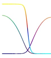
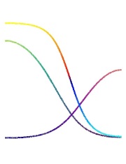
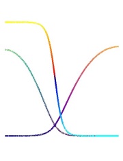
Figure 1 shows snapshots of the time evolution in the case of no oscillations in either diffusion coefficient, i.e., A(y)=B(y)=2𝐴𝑦𝐵𝑦2A(y)=B(y)=2 with ε=103𝜀superscript103\varepsilon=10^{-3}. We observe spatial segregation due to the strong competition and due to its competitive advantage the species uεsuperscript𝑢𝜀u^{\varepsilon} invades the habitat of the species vεsuperscript𝑣𝜀v^{\varepsilon}. The long time behaviour being complete colonisation of ΩΩ\Omega by the species uεsuperscript𝑢𝜀u^{\varepsilon} and the extinction of the species vεsuperscript𝑣𝜀v^{\varepsilon}.

Refer to caption

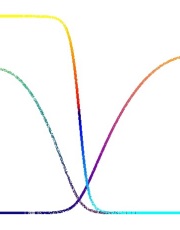
Refer to caption Refer to caption Refer to caption Refer to caption Refer to caption

Figure 1. Snapshots of the solution to (26) with constant diffusion coefficients A(y)=B(y)=2𝐴𝑦𝐵𝑦2A(y)=B(y)=2 and α=1.1𝛼1.1\alpha=1.1 at times 0.1,0.3,0.4,0.50.10.30.40.50.1,0.3,0.4,0.5 and 0.60.60.6 reading from left to right. We observe that due to the competitive advantage species uεsuperscript𝑢𝜀u^{\varepsilon} invades the habitat of species vεsuperscript𝑣𝜀v^{\varepsilon}.

In order to illustrate the effect of high frequency oscillations we now consider the periodic diffusivities associated with the two population densities in (26) taken to be

(27) A(y)=2+1.5sin(2πy)B(y)=2} for yY.cases𝐴𝑦absent21.52𝜋𝑦𝐵𝑦absent2 for 𝑦𝑌\left.\begin{array}[]{rl}A(y)&=2+1.5\sin(2\pi y)\\[5.69046pt] B(y)&=2\end{array}\right\}\quad\mbox{ for }y\in Y.

The associated homogenized coefficients in Theorem 13 (see in particular (11) and (33)) are given as

Ahom=1.3229Bhom=2.subscript𝐴homabsent1.3229subscript𝐵homabsent2\begin{array}[]{rl}A_{\rm hom}&=1.3229\\[5.69046pt] B_{\rm hom}&=2.\end{array}

Note that the above choice of periodic diffusivities are such that

A(y)>B(y) for y(0,12)A(y)<B(y) for y(12,1),𝐴𝑦𝐵𝑦 for 𝑦012𝐴𝑦𝐵𝑦 for 𝑦121\begin{array}[]{cl}A(y)>B(y)&\mbox{ for }y\in\left(0,\frac{1}{2}\right)\\[5.69046pt] A(y)<B(y)&\mbox{ for }y\in\left(\frac{1}{2},1\right),\end{array}

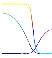
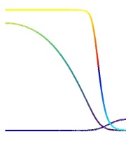
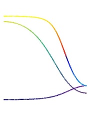
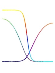
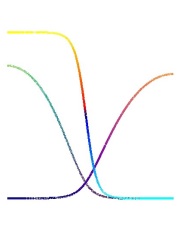
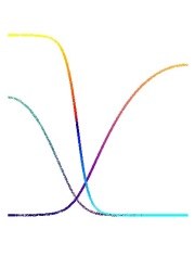
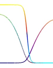
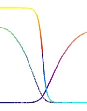
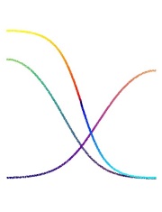
i.e., the dominance of one diffusion coefficient over the other inside a periodicity cell is symmetric. But the high frequency oscillations in the homogenization limit lead to coefficients such that Ahom<Bhomsubscript𝐴homsubscript𝐵homA_{\rm hom}<B_{\rm hom} everywhere in the spatial domain. Figure 2 shows snapshots of the time evolution in the case of diffusivities as in (27) for varying ε𝜀\varepsilon. We see that for sufficiently small ε𝜀\varepsilon the long-time behaviour of the system changes from the constant diffusion case with the species with constant diffusivity invading the habitat of the species with oscillating diffusivity even though the species with oscillating diffusivity has a competitive advantage over the other.

Refer to caption

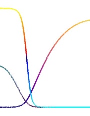
Refer to caption Refer to caption Refer to caption Refer to caption Refer to caption Refer to caption Refer to caption Refer to caption Refer to caption Refer to caption Refer to caption Refer to caption Refer to caption Refer to caption Refer to caption Refer to caption Refer to caption

Figure 2. Snapshots of the solution to (26) with ε=102𝜀superscript102\varepsilon=10^{-2} (top row), 2×1032superscript1032\times 10^{-3} (middle row) and 103superscript10310^{-3} (bottom row) at times 0.1,0.3,0.4,0.50.10.30.40.50.1,0.3,0.4,0.5 and 0.60.60.6 reading from left to right in each row. The diffusion coefficients are as in (27) and we set α=1.1𝛼1.1\alpha=1.1. We observe that despite the competitive advantage , due to the high frequency oscillations, the species vεsuperscript𝑣𝜀v^{\varepsilon} invades the habitat of species uεsuperscript𝑢𝜀u^{\varepsilon} for the cases of ε=2×10³𝜀2superscript103\varepsilon=2\times 10^{-3} and ε=103𝜀superscript103\varepsilon=10^{-3}.

4.2. 2D Simulations

Thus far, we treated only the one-dimensional setting. In the example to follow, we consider (26) on a two-dimensional setting with the spatial domain Ω:=(0,1)2assignΩsuperscript012\Omega:=(0,1)^{2}. We fix α=1.1𝛼1.1\alpha=1.1, λ=1𝜆1\lambda=1 and r=50𝑟50r=50 and start by considering the constant diffusion case, i.e, the periodic diffusivities associated with the species uεsuperscript𝑢𝜀u^{\varepsilon} and vεsuperscript𝑣𝜀v^{\varepsilon} are

A(y1,y2)=B(y1,y2)=2Id.𝐴subscript𝑦1subscript𝑦2𝐵subscript𝑦1subscript𝑦22IdA(y_{1},y_{2})=B(y_{1},y_{2})=2\,\,{\rm Id}.

For the initial conditions we set

uin(x1,x2)superscript𝑢insubscript𝑥1subscript𝑥2\displaystyle u^{\rm in}(x_{1},x_{2}) =χ{x1+0.1sin(2πx2)<0.5}absentsubscript𝜒subscript𝑥10.12𝜋subscript𝑥20.5\displaystyle=\chi_{\{x_{1}+0.1\sin(2\pi x_{2})<0.5\}}
vin(x1,x2)superscript𝑣insubscript𝑥1subscript𝑥2\displaystyle v^{\rm in}(x_{1},x_{2}) =χ{x1+0.1sin(2πx2)0.5}absentsubscript𝜒subscript𝑥10.12𝜋subscript𝑥20.5\displaystyle=\chi_{\{x_{1}+0.1\sin(2\pi x_{2})\geq 0.5\}}
win(x)superscript𝑤in𝑥\displaystyle w^{\rm in}(x) =uin(x)absentsuperscript𝑢in𝑥\displaystyle=u^{\rm in}(x)

for xΩ𝑥Ωx\in\Omega. For the simulations we employ a uniform mesh with 2099201 degrees of freedom (a fine mesh is needed to resolve the highly oscillatory diffusion coefficient) and a fixed timestep of 103superscript10310^{-3}.

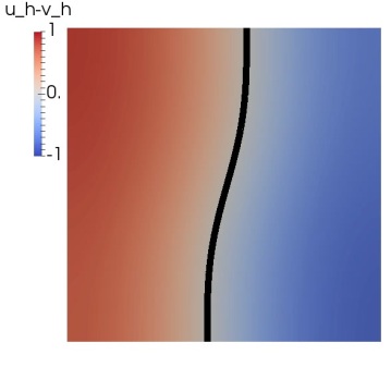
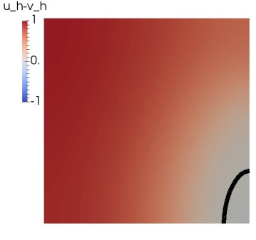
Figure 3 shows snapshots of the time evolution in this case. We report on the difference between uεsuperscript𝑢𝜀u^{\varepsilon} and vεsuperscript𝑣𝜀v^{\varepsilon} and indicate the zero contour of this difference. Due to its competitive advantage the species uεsuperscript𝑢𝜀u^{\varepsilon} invades the habitat of the species vεsuperscript𝑣𝜀v^{\varepsilon}. The long time behaviour is the complete colonisation of ΩΩ\Omega by the species uεsuperscript𝑢𝜀u^{\varepsilon} and the extinction of the species vεsuperscript𝑣𝜀v^{\varepsilon}.

Refer to caption Refer to caption Refer to caption

Figure 3. Snapshots of the solution to (26) with constant diffusivities, λ=1𝜆1\lambda=1, r=50𝑟50r=50 and α=1.1𝛼1.1\alpha=1.1 at times 0.1,0.30.10.30.1,0.3 and 0.50.50.5 reading from left to right. We observe that due to the competitive advantage species uεsuperscript𝑢𝜀u^{\varepsilon} invades the habitat of species vεsuperscript𝑣𝜀v^{\varepsilon}.

As above, to illustrate the effect of oscillations, we now consider the periodic diffusivity associated with uεsuperscript𝑢𝜀u^{\varepsilon} to be

A(y1,y2)=(2+1.5sin(2πy1)002)𝐴subscript𝑦1subscript𝑦2matrix21.52𝜋subscript𝑦1002\displaystyle A(y_{1},y_{2})=\left(\begin{matrix}2+1.5\sin(2\pi y_{1})&0\\[5.69046pt] 0&2\end{matrix}\right)

and that associated with the population density vεsuperscript𝑣𝜀v^{\varepsilon} to be

B(y1,y2)=2Id.𝐵subscript𝑦1subscript𝑦22Id\displaystyle B(y_{1},y_{2})=2\,\,{\rm Id}.

The associated homogenized matrices (using Corollary 19) are

Ahom=(1.3229002) and Bhom=2Id.formulae-sequencesubscript𝐴hommatrix1.3229002 and subscript𝐵hom2Id\displaystyle A_{\rm hom}=\left(\begin{matrix}1.3229&0\\[5.69046pt] 0&2\end{matrix}\right)\quad\text{ and }\quad B_{\rm hom}=2\,\,{\rm Id}.

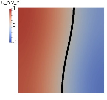
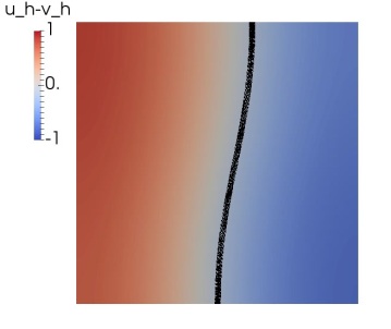
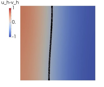
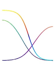
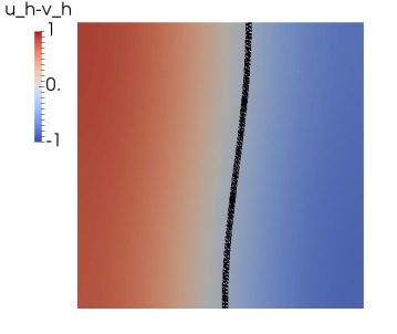
Figure 4 shows snapshots of the time evolution in this case of oscillating diffusivity with ε=2×10³𝜀2superscript103\varepsilon=2\times 10^{-3} for one of the species. We see that the behaviour of the system appears to change from the constant diffusion case with the direction of motion of the front between the two species being reversed and the species with constant diffusivity invading the habitat of the species with oscillating diffusivity even though the species with oscillating diffusivity has a competitive advantage over the other.
Refer to caption Refer to caption Refer to caption

Figure 4. Snapshots of the solution to (26) with oscillating diffusivity for one species with ε=2×10³𝜀2superscript103\varepsilon=2\times 10^{-3}, λ=1𝜆1\lambda=1, r=50𝑟50r=50 and α=1.1𝛼1.1\alpha=1.1 at times 0.1,0.40.10.40.1,0.4 and 111 reading from left to right. We observe that despite the fact that uεsuperscript𝑢𝜀u^{\varepsilon} enjoys a competitive advantage over vεsuperscript𝑣𝜀v^{\varepsilon}, due to oscillations in the diffusivity of uεsuperscript𝑢𝜀u^{\varepsilon}, the species vεsuperscript𝑣𝜀v^{\varepsilon} invades the habitat of species uεsuperscript𝑢𝜀u^{\varepsilon}.

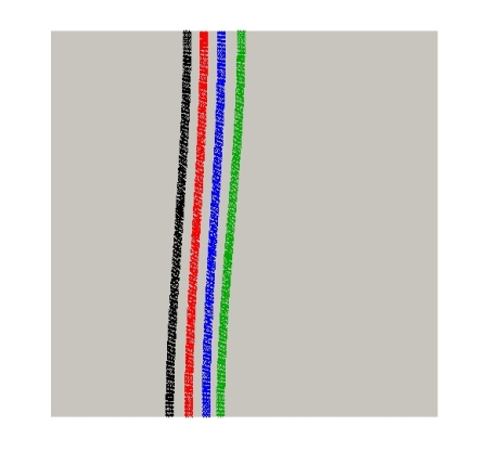
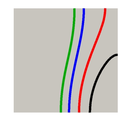
To illustrate this reversal in the invasion behaviour more clearly, in Figure 5, we plot the position of the front at a series of times in the case of constant diffusivities and in the case of oscillating diffusivity for uεsuperscript𝑢𝜀u^{\varepsilon} and constant diffusivity for vεsuperscript𝑣𝜀v^{\varepsilon}. The reversal in invasion behaviour is clearly evident.
Refer to caption    Refer to caption


Figure 5. Left: position of the front between the two species habitats ({uε=vε}superscript𝑢𝜀superscript𝑣𝜀\{u^{\varepsilon}=v^{\varepsilon}\}), in the case of constant diffusivities for both species, at t=0.1𝑡0.1t=0.1 (green), 0.30.30.3 (blue), 0.40.40.4 (red) and 0.450.450.45 (black). We observe that the front moves towards the right hand boundary as species uεsuperscript𝑢𝜀u^{\varepsilon} invades the habitat of vεsuperscript𝑣𝜀v^{\varepsilon}. Right: position of the front between the two species habitats ({uε=vε}superscript𝑢𝜀superscript𝑣𝜀\{u^{\varepsilon}=v^{\varepsilon}\}), in the case of oscillating diffusivity for uεsuperscript𝑢𝜀u^{\varepsilon} and constant diffusivity for vεsuperscript𝑣𝜀v^{\varepsilon}, at t=0.65𝑡0.65t=0.65 (green), 0.850.850.85 (blue), 0.950.950.95 (red) and 111 (black). We observe that the direction of motion of the front is reversed s the species vεsuperscript𝑣𝜀v^{\varepsilon} invades the habitat of uεsuperscript𝑢𝜀u^{\varepsilon}.
Remark 18.

The aforementioned 2D2𝐷2D simulations bear some similarity to the simulations in [DHMP99, pp.100–101]. However, the scenario in [DHMP99] is to consider isotropic diffusivities in the ε𝜀\varepsilon-problem. So, our work is slightly different in that we need to consider anisotropic diffusion and also the work in [DHMP99] does not show any simulations to study the t1much-greater-than𝑡1t\gg 1 regime.

5. Different scales for diffusion and competition

We can take a different view in comparison to the calculations presented thus far. In the competition-diffusion model (1), the periodic oscillations in the diffusivities are of frequency ε𝜀\varepsilon and the competition rate is of 𝒪(ε1)𝒪superscript𝜀1\mathcal{O}(\varepsilon^{-1}). To present quite a general scenario, let ε𝜀\varepsilon denote the characteristic length of the inhomogeneities and let δ𝛿\delta denote a parameter such that the competition rate is of 𝒪(δ1)𝒪superscript𝛿1\mathcal{O}(\delta^{-1}). As we are considering two parameters, we denote the population densities uε,δ(t,x)superscript𝑢𝜀𝛿𝑡𝑥u^{\varepsilon,\delta}(t,x) and vε,δ(t,x)superscript𝑣𝜀𝛿𝑡𝑥v^{\varepsilon,\delta}(t,x) which satisfy the competition-diffusion model

(28) tuε,δ(Aε(x)uε,δ)+uε,δδ(vε,δ+λ(1wε,δ))subscript𝑡superscript𝑢𝜀𝛿superscript𝐴𝜀𝑥superscript𝑢𝜀𝛿superscript𝑢𝜀𝛿𝛿superscript𝑣𝜀𝛿𝜆1superscript𝑤𝜀𝛿\displaystyle\partial_{t}u^{\varepsilon,\delta}-\nabla\cdot\Big{(}A^{\varepsilon}(x)\nabla u^{\varepsilon,\delta}\Big{)}+\frac{u^{\varepsilon,\delta}}{\delta}\Big{(}v^{\varepsilon,\delta}+\lambda\left(1-w^{\varepsilon,\delta}\right)\Big{)} =0absent0\displaystyle=0 in (0,)×Ω,in 0Ω\displaystyle\mbox{ in }(0,\ell)\times\Omega,
tvε,δ(Bε(x)vε,δ)+αvε,δδ(uε,δ+λwε,δ)subscript𝑡superscript𝑣𝜀𝛿superscript𝐵𝜀𝑥superscript𝑣𝜀𝛿𝛼superscript𝑣𝜀𝛿𝛿superscript𝑢𝜀𝛿𝜆superscript𝑤𝜀𝛿\displaystyle\partial_{t}v^{\varepsilon,\delta}-\nabla\cdot\Big{(}B^{\varepsilon}(x)\nabla v^{\varepsilon,\delta}\Big{)}+\alpha\frac{v^{\varepsilon,\delta}}{\delta}\Big{(}u^{\varepsilon,\delta}+\lambda w^{\varepsilon,\delta}\Big{)} =0absent0\displaystyle=0 in (0,)×Ω,in 0Ω\displaystyle\mbox{ in }(0,\ell)\times\Omega,
twε,δ+uε,δδ(wε,δ1)+wε,δvε,δδsubscript𝑡superscript𝑤𝜀𝛿superscript𝑢𝜀𝛿𝛿superscript𝑤𝜀𝛿1superscript𝑤𝜀𝛿superscript𝑣𝜀𝛿𝛿\displaystyle\partial_{t}w^{\varepsilon,\delta}+\frac{u^{\varepsilon,\delta}}{\delta}\left(w^{\varepsilon,\delta}-1\right)+\frac{w^{\varepsilon,\delta}v^{\varepsilon,\delta}}{\delta} =0absent0\displaystyle=0 in (0,)×Ω.in 0Ω\displaystyle\mbox{ in }(0,\ell)\times\Omega.

The evolution system (28) for (uε,δ,vε,δ,wε,δ)superscript𝑢𝜀𝛿superscript𝑣𝜀𝛿superscript𝑤𝜀𝛿\left(u^{\varepsilon,\delta},v^{\varepsilon,\delta},w^{\varepsilon,\delta}\right) is supplemented by initial and boundary conditions

(29) uε,δ(0,x)=uin(x),vε,δ(0,x)=vin(x),wε,δ(0,x)=win(x)formulae-sequencesuperscript𝑢𝜀𝛿0𝑥superscript𝑢in𝑥formulae-sequencesuperscript𝑣𝜀𝛿0𝑥superscript𝑣in𝑥superscript𝑤𝜀𝛿0𝑥superscript𝑤in𝑥\displaystyle u^{\varepsilon,\delta}(0,x)=u^{\rm in}(x),\,v^{\varepsilon,\delta}(0,x)=v^{\rm in}(x),\,w^{\varepsilon,\delta}(0,x)=w^{\rm in}(x) in Ωin Ω\displaystyle\mbox{ in }\Omega
Aε(x)uε,δ𝐧(x)=Bε(x)vε,δ𝐧(x)superscript𝐴𝜀𝑥superscript𝑢𝜀𝛿𝐧𝑥superscript𝐵𝜀𝑥superscript𝑣𝜀𝛿𝐧𝑥\displaystyle A^{\varepsilon}(x)\nabla u^{\varepsilon,\delta}\cdot{\bf n}(x)=B^{\varepsilon}(x)\nabla v^{\varepsilon,\delta}\cdot{\bf n}(x) =0absent0\displaystyle=0 on (0,)×Ω.on 0Ω\displaystyle\mbox{ on }(0,\ell)\times\partial\Omega.

The calculations presented so far treat the case ε=δ𝜀𝛿\varepsilon=\delta. In this section, we comment on two other cases: (i) εδmuch-less-than𝜀𝛿\varepsilon\ll\delta and (ii) δεmuch-less-than𝛿𝜀\delta\ll\varepsilon.
In the regime εδmuch-less-than𝜀𝛿\varepsilon\ll\delta, for any fixed δ>0𝛿0\delta>0, the ε0𝜀0\varepsilon\to 0 limit takes over, i.e., the homogenization limit dominates the competition limit. More precisely, fixing a δ>0𝛿0\delta>0, the family (uε,δ,vε,δ,wε,δ)superscript𝑢𝜀𝛿superscript𝑣𝜀𝛿superscript𝑤𝜀𝛿\left(u^{\varepsilon,\delta},v^{\varepsilon,\delta},w^{\varepsilon,\delta}\right) has a limit point (u,δ,v,δ,w,δ)superscript𝑢𝛿superscript𝑣𝛿superscript𝑤𝛿\left(u^{\ast,\delta},v^{\ast,\delta},w^{\ast,\delta}\right) satisfying

(30) tu,δ(Ahomu,δ)+u,δδ(v,δ+λ(1w,δ))subscript𝑡superscript𝑢𝛿subscript𝐴homsuperscript𝑢𝛿superscript𝑢𝛿𝛿superscript𝑣𝛿𝜆1superscript𝑤𝛿\displaystyle\partial_{t}u^{\ast,\delta}-\nabla\cdot\Big{(}A_{\rm hom}\nabla u^{\ast,\delta}\Big{)}+\frac{u^{\ast,\delta}}{\delta}\Big{(}v^{\ast,\delta}+\lambda\left(1-w^{\ast,\delta}\right)\Big{)} =0absent0\displaystyle=0 in (0,)×Ω,in 0Ω\displaystyle\mbox{ in }(0,\ell)\times\Omega,
tv,δ(Bhomv,δ)+αv,δδ(u,δ+λw,δ)subscript𝑡superscript𝑣𝛿subscript𝐵homsuperscript𝑣𝛿𝛼superscript𝑣𝛿𝛿superscript𝑢𝛿𝜆superscript𝑤𝛿\displaystyle\partial_{t}v^{\ast,\delta}-\nabla\cdot\Big{(}B_{\rm hom}\nabla v^{\ast,\delta}\Big{)}+\alpha\frac{v^{\ast,\delta}}{\delta}\Big{(}u^{\ast,\delta}+\lambda w^{\ast,\delta}\Big{)} =0absent0\displaystyle=0 in (0,)×Ω,in 0Ω\displaystyle\mbox{ in }(0,\ell)\times\Omega,
tw,δ+u,δδ(w,δ1)+w,δv,δδsubscript𝑡superscript𝑤𝛿superscript𝑢𝛿𝛿superscript𝑤𝛿1superscript𝑤𝛿superscript𝑣𝛿𝛿\displaystyle\partial_{t}w^{\ast,\delta}+\frac{u^{\ast,\delta}}{\delta}\left(w^{\ast,\delta}-1\right)+\frac{w^{\ast,\delta}v^{\ast,\delta}}{\delta} =0absent0\displaystyle=0 in (0,)×Ω.in 0Ω\displaystyle\mbox{ in }(0,\ell)\times\Omega.

The homogenization procedure is exactly similar to the one present in the proof of Theorem 13. The main ingredient being the compactness properties of the family (uε,δ,vε,δ,wε,δ)superscript𝑢𝜀𝛿superscript𝑣𝜀𝛿superscript𝑤𝜀𝛿\left(u^{\varepsilon,\delta},v^{\varepsilon,\delta},w^{\varepsilon,\delta}\right) as given in (7). The limit equation obtained above for (u,δ,v,δ,w,δ)superscript𝑢𝛿superscript𝑣𝛿superscript𝑤𝛿\left(u^{\ast,\delta},v^{\ast,\delta},w^{\ast,\delta}\right) is treated similar to the one treated in [HIMN01] in the δ0𝛿0\delta\to 0 limit which corresponds to the strong competition limit. Finally, the obtained limit is exactly the same as the limit equation (10) as in Theorem 13.
In the regime δεmuch-less-than𝛿𝜀\delta\ll\varepsilon, the roles are reversed, i.e., for any fixed ε>0𝜀0\varepsilon>0, the δ0𝛿0\delta\to 0 limit takes over, i.e., the competition limit dominates homogenization limit. More precisely, fixing a ε>0𝜀0\varepsilon>0, the family (uε,δ,vε,δ,wε,δ)superscript𝑢𝜀𝛿superscript𝑣𝜀𝛿superscript𝑤𝜀𝛿\left(u^{\varepsilon,\delta},v^{\varepsilon,\delta},w^{\varepsilon,\delta}\right) has a limit point (uε,,vε,,wε,)superscript𝑢𝜀superscript𝑣𝜀superscript𝑤𝜀\left(u^{\varepsilon,\ast},v^{\varepsilon,\ast},w^{\varepsilon,\ast}\right) satisfying a two-phase Stefan problem with oscillating diffusivities Aε(x)superscript𝐴𝜀𝑥A^{\varepsilon}(x) and Bε(x)superscript𝐵𝜀𝑥B^{\varepsilon}(x). The homogenization of two-phase and single-phase Stefan-type equations has received a lot of attention. Here we cite a few which can be used to homogenize our limit equation for (uε,,vε,,wε,)superscript𝑢𝜀superscript𝑣𝜀superscript𝑤𝜀\left(u^{\varepsilon,\ast},v^{\varepsilon,\ast},w^{\varepsilon,\ast}\right). Here are the references: [Rod82, Vis07, KM08, KM10].

In full generality, one could consider the two scaling parameters ε𝜀\varepsilon and δ𝛿\delta to be related via a relation δ=εβ𝛿superscript𝜀𝛽\delta=\varepsilon^{\beta} with β(0,)𝛽0\beta\in(0,\infty). It could be of interest, both from the mathematical and applications perspective, to check the feasibility of arriving a result similar in flavour to Theorem 13 for a range of values of the exponent β𝛽\beta. Here we cite [BH16] where a similar question was addressed in the context of simultaneous diffusion and homogenization approximation for the linear Boltzmann equation from kinetic theory. The present scenario, however, is a bit subtle as our competition-diffusion model is nonlinear and as there is species segregation in the limit problem. This analysis in a more general setting is quite intricate and is left for future investigations.

Appendix A One dimensional and layered materials

As an illustrative example, let us consider the particular one-dimensional setting, i.e., when d=1𝑑1d=1 and when the reference periodicity cell Y:=[0,1)assign𝑌01Y:=[0,1). Let us denote the periodic one-dimensional conductivity coefficient as a(y)𝑎𝑦a(y) and the associated homogenized coefficient as ahomsubscript𝑎homa_{\rm hom}. In this scenario, the cell problem (23) is to solve for a 111-periodic function η(y)𝜂𝑦\eta(y) such that

(31) ddy(a(y)(1+dη(y)dy))=0 in (0,1).dd𝑦𝑎𝑦1d𝜂𝑦d𝑦0 in 01\displaystyle\frac{\rm d}{{\rm d}y}\Big{(}a(y)\Big{(}1+\frac{{\rm d}\eta(y)}{{\rm d}y}\Big{)}\Big{)}=0\quad\mbox{ in }(0,1).

Integrating the differential equation (31) yields

(32) a(y)(1+dη(y)dy)=𝖼1𝑎𝑦1d𝜂𝑦d𝑦subscript𝖼1\displaystyle a(y)\Big{(}1+\frac{{\rm d}\eta(y)}{{\rm d}y}\Big{)}=\mathsf{c}_{1}

with 𝖼1subscript𝖼1\mathsf{c}_{1} being the integrating constant. Integrating (32) over (0,y)0𝑦(0,y) yields

(y+η(y))=𝖼2+0y𝖼1a(y)dy𝑦𝜂𝑦subscript𝖼2superscriptsubscript0𝑦subscript𝖼1𝑎superscript𝑦differential-dsuperscript𝑦\displaystyle\Big{(}y+\eta(y)\Big{)}=\mathsf{c}_{2}+\int\limits_{0}^{y}\frac{\mathsf{c}_{1}}{a(y^{\prime})}\,{\rm d}y^{\prime}

for another integrating constant 𝖼2subscript𝖼2\mathsf{c}_{2}. Using the periodic-boundary condition on η(y)𝜂𝑦\eta(y), we determine the constant 𝖼1subscript𝖼1\mathsf{c}_{1} as

𝖼101dya(y)=1.subscript𝖼1superscriptsubscript01d𝑦𝑎𝑦1\displaystyle\mathsf{c}_{1}\int\limits_{0}^{1}\frac{{\rm d}y}{a(y)}=1.

The expression for the homogenized coefficient in (25) becomes

ahom=01a(y)(1+dη(y)dy)dy.subscript𝑎homsuperscriptsubscript01𝑎𝑦1d𝜂𝑦d𝑦differential-d𝑦\displaystyle a_{\rm hom}=\int\limits_{0}^{1}a(y)\Big{(}1+\frac{{\rm d}\eta(y)}{{\rm d}y}\Big{)}\,{\rm d}y.

The observation (32) straightaway implies that

(33) ahom01dya(y)=1,subscript𝑎homsuperscriptsubscript01d𝑦𝑎𝑦1\displaystyle a_{\rm hom}\int\limits_{0}^{1}\frac{{\rm d}y}{a(y)}=1,

i.e., the homogenized coefficient ahomsubscript𝑎homa_{\rm hom} is nothing but the harmonic average of the conductivity coefficient a(y)𝑎𝑦a(y) over the period.
As the above calculations suggest, one can give an explicit analytical expression for the homogenized coefficient in one-dimensional periodic settings. Under some specific assumptions (such as the layered materials), explicit analytical expressions can be derived for the associated homogenized coefficient (for further details, see for e.g., [All02, Chapter 1], [CD99, Chapter 5] & [PS08, Chapter 12] and references therein). For readers convenience, we gather a result on layered materials in two dimensions (see [PS08, pp. 193–195] for details).

Corollary 19.

Take the periodicity reference cell Y:=[0,1)2assign𝑌superscript012Y:=[0,1)^{2} and take the periodic diffusivity 𝒜(y)𝒜𝑦\mathcal{A}(y) in Theorem 17 to be

𝒜(y1,y2)=(𝒜11(y1)𝒜12(y1)𝒜21(y1)𝒜22(y1)).𝒜subscript𝑦1subscript𝑦2matrixsubscript𝒜11subscript𝑦1subscript𝒜12subscript𝑦1subscript𝒜21subscript𝑦1subscript𝒜22subscript𝑦1\displaystyle\mathcal{A}(y_{1},y_{2})=\left(\begin{matrix}\mathcal{A}_{11}(y_{1})&\mathcal{A}_{12}(y_{1})\\[5.69046pt] \mathcal{A}_{21}(y_{1})&\mathcal{A}_{22}(y_{1})\end{matrix}\right).

The associated homogenized matrix 𝒜homsubscript𝒜hom\mathcal{A}_{\rm hom} is given below

[𝒜hom]1101dy1𝒜11(y1)=1;[𝒜hom]1201dy1𝒜11(y1)=01𝒜12(y1)𝒜11(y1)dy1;formulae-sequencesubscriptdelimited-[]subscript𝒜hom11superscriptsubscript01dsubscript𝑦1subscript𝒜11subscript𝑦11subscriptdelimited-[]subscript𝒜hom12superscriptsubscript01dsubscript𝑦1subscript𝒜11subscript𝑦1superscriptsubscript01subscript𝒜12subscript𝑦1subscript𝒜11subscript𝑦1differential-dsubscript𝑦1\displaystyle\left[\mathcal{A}_{\rm hom}\right]_{11}\int\limits_{0}^{1}\frac{{\rm d}y_{1}}{\mathcal{A}_{11}(y_{1})}=1;\qquad\left[\mathcal{A}_{\rm hom}\right]_{12}\int\limits_{0}^{1}\frac{{\rm d}y_{1}}{\mathcal{A}_{11}(y_{1})}=\int\limits_{0}^{1}\frac{\mathcal{A}_{12}(y_{1})}{\mathcal{A}_{11}(y_{1})}\,{\rm d}y_{1};
[𝒜hom]2101dy1𝒜11(y1)subscriptdelimited-[]subscript𝒜hom21superscriptsubscript01dsubscript𝑦1subscript𝒜11subscript𝑦1\displaystyle\left[\mathcal{A}_{\rm hom}\right]_{21}\int\limits_{0}^{1}\frac{{\rm d}y_{1}}{\mathcal{A}_{11}(y_{1})} =01𝒜21(y1)𝒜11(y1)dy1;absentsuperscriptsubscript01subscript𝒜21subscript𝑦1subscript𝒜11subscript𝑦1differential-dsubscript𝑦1\displaystyle=\int\limits_{0}^{1}\frac{\mathcal{A}_{21}(y_{1})}{\mathcal{A}_{11}(y_{1})}\,{\rm d}y_{1};
[𝒜hom]2201dy1𝒜11(y1)=subscriptdelimited-[]subscript𝒜hom22superscriptsubscript01dsubscript𝑦1subscript𝒜11subscript𝑦1absent\displaystyle\left[\mathcal{A}_{\rm hom}\right]_{22}\int\limits_{0}^{1}\frac{{\rm d}y_{1}}{\mathcal{A}_{11}(y_{1})}= (01𝒜21(y1)𝒜11(y1)dy1)(01𝒜12(y1)𝒜11(y1)dy1)superscriptsubscript01subscript𝒜21subscript𝑦1subscript𝒜11subscript𝑦1differential-dsubscript𝑦1superscriptsubscript01subscript𝒜12subscript𝑦1subscript𝒜11subscript𝑦1differential-dsubscript𝑦1\displaystyle\left(\int\limits_{0}^{1}\frac{\mathcal{A}_{21}(y_{1})}{\mathcal{A}_{11}(y_{1})}\,{\rm d}y_{1}\right)\left(\int\limits_{0}^{1}\frac{\mathcal{A}_{12}(y_{1})}{\mathcal{A}_{11}(y_{1})}\,{\rm d}y_{1}\right)
+(01dy1𝒜11(y1))(01(𝒜22(y1)𝒜12(y1)𝒜21(y1)𝒜11(y1))dy1).superscriptsubscript01dsubscript𝑦1subscript𝒜11subscript𝑦1superscriptsubscript01subscript𝒜22subscript𝑦1subscript𝒜12subscript𝑦1subscript𝒜21subscript𝑦1subscript𝒜11subscript𝑦1differential-dsubscript𝑦1\displaystyle+\left(\int\limits_{0}^{1}\frac{{\rm d}y_{1}}{\mathcal{A}_{11}(y_{1})}\right)\left(\int\limits_{0}^{1}\left(\mathcal{A}_{22}(y_{1})-\frac{\mathcal{A}_{12}(y_{1})\mathcal{A}_{21}(y_{1})}{\mathcal{A}_{11}(y_{1})}\right)\,{\rm d}y_{1}\right).

References