Analytical description of the survival probability of coherent states in regular regimes

Abstract

Using coherent states as initial states, we investigate the quantum dynamics of the Lipkin-Meshkov-Glick (LMG) and Dicke models in the semi-classical limit. They are representative models of bounded systems with one- and two-degrees of freedom, respectively. The first model is integrable, while the second one has both regular and chaotic regimes. Our analysis is based on the survival probability. Within the regular regime, the energy distribution of the initial coherent states consists of quasi-harmonic sub-sequences of energies with Gaussian weights. This allows for the derivation of analytical expressions that accurately describe the entire evolution of the survival probability, from $t=0$ to the saturation of the dynamics. The evolution shows decaying oscillations with a rate that depends on the anharmonicity of the spectrum and, in the case of the Dicke model, on interference terms coming from the simultaneous excitation of its two-degrees of freedom. As we move away from the regular regime, the complexity of the survival probability is shown to be closely connected with the properties of the corresponding classical phase space. Our approach has broad applicability, since its central assumptions are not particular of the studied models.

Keywords Quantum dynamics, survival probability, semi-classical approximation, Dicke model, Lipkin-Meshkov-Glick model.

I Introduction

Highly controllable experiments with cold atoms Chu2002 ; BernienARXIV , ion traps Blatt2012 ; Richerme2014 , and nuclear magnetic resonance (NMR) platforms WeiARXIV , where coherent evolution can be investigated for long times, are in part responsible for the renewed interest in non-equilibrium quantum dynamics. Alongside with several paradigmatic models of many-body quantum physics, simple but rich ones like the Lipkin-Meshkov-Glick (LMG) Lipkin1965a ; Lipkin1965b ; Lipkin1965c and the Dicke Dicke54 ; Hepp73 ; Wang1973 models have become experimentally accessible. The latter were realized with Bose-Einstein condensates in  Milburn1997 ; Steel1998 ; Zibold2010 and  Baumann2010 ; Baumann2011 , respectively.

To better understand and control many-body quantum systems out of equilibrium, in addition to experimental and numerical studies, one can exploit the advantages of analytical results to identify and explain the causes of different behaviors at different time scales. However, analytical results are challenging in systems that approach chaotic regimes.

The present work focuses on the analytical description of the equilibration process of the LMG and Dicke models. They are representative models of bounded systems with one- and two-degrees of freedom, respectively (the number of degrees of freedom defined through the classical limit). The LMG model is integrable, while the Dicke model presents both regular and chaotic classical trajectories. Our analysis concentrates on the regular regime, which enables the derivation of analytical expressions that cover the entire dynamics of the two systems. In the case of the Dicke model, by gradually moving the initial state away from the regular regime, we are able to identify the source of the increased complexity of the dynamics.

The quantity that we select for our studies is the survival probability ($SP$), that is the probability of finding the initial state later in time. $SP$ is a simple dynamical quantity that encodes the structure of the energy components of the initial state, making it a valuable tool to detect and study critical phenomena in the energy spectrum, such as quantum phase transitions (QPT) Campbell16 , excited-state quantum phase transitions (ESQPT) Wang17 ; SantosBernal2015 ; Santos2016 ; Fernandez2011 and dynamical phase transitions DQPT ; DQPT2 ; correlations in the energy spectrum that distinguish between regular and chaotic systems Alhassid92 ; Torres2017b ; decay of unstable systems Fonda78 ; metal-insulator transition Ketz92 ; and quantum speed limit Khalfin58 , among other subjects.

The survival probability (also known as return probability) and the Loschmidt echo Peres1984 ; Gorin2006 are particular cases of the fidelity between two pure states. While the survival probability measures the overlap between the initial state and its evolved counterpart, the Loschmidt echo evaluates the overlap between the initial state evolved under two different Hamiltonians. In the scenario of small perturbations, where the two Hamiltonians are only slightly different, analytical expressions for the Loschmidt echo have been obtained Prosen2002 ; Prosen2003 . We stress that our focus is on the survival probability and on very strong perturbations that take the system far from equilibrium.

As discussed in previous works, at short times the $SP$ shows a universal quadratic decay with rate determined by the energy variance of the initial state. Its subsequent decay is controlled by the shape of the energy distribution, Gaussian and exponential behaviors being common for strong perturbations *Torres2014PRA; *Torres2014NJP; *Torres2014PRE; Torres2014PRAb ; Flamabum2001 ; Izrailev2006 . At later times, the $SP$ behavior is rather complex, depending strongly on the details of the energy components probed by the initial state *Tavora2016; *Tavora2017; Alhassid92 ; Torres2017 . For finite-size systems the $SP$ eventually saturates to its infinite-time average at the equilibration time, showing fluctuations whose temporal dispersion is of the order of the saturation value.

In the present paper, the $SP$ is used to describe in detail the different temporal scales in the equilibration process of regular quantum systems with few-degrees of freedom and with a well defined classical limit. To gain insights from the classical dynamics, we use coherent states KlauderBook ; Gilmore90 as initial states and consider a small effective Planck constant Altland2012NJP ; Altland2012PRL ; Bakemeier13 .

Our approach finds inspiration in the study of multilevel quantum beats in Leichtle1996 . We identify the relevant properties of the initial state and the energy spectrum responsible for the dynamic behaviors observed at different times. This analysis enables us to provide a precise definition of the equilibration time. We stress that our approach can be extended to other similar models where the spectrum has a regular part. It was indeed recently employed in Kloc18 for the analysis of the quenched dynamics of the integrable two-degrees of freedom Tavis-Cummings model and in HUMBERTO for a one-dimensional quartic double-well potential in the semi-classical limit.

In the LMG model, the analytical expression that we obtain for the $SP(t)$ is a sum of products of cosine and Gaussian functions. It depends only on three parameters that can be estimated analytically and semi-classically. The decay rate of the oscillations of the $SP(t)$ is proportional to the anharmonicity of the spectrum probed by the initial state. In the Dicke model, since the regular part of the energy spectrum is organized in invariant subspaces associated with the quantum numbers of approximate integrals of motion Relano16 ; BastaJPA17 , instead of a single sum, the analytical expression for the $SP(t)$ consists of different sums and interferences between them. The number of sums grows as the energy and parameters of the initial coherent state approach chaotic classical regions. This causes the decay time of the oscillations to decrease significantly. For both models, the analytical results are compared with numerics, showing remarkable agreement.

The paper is organized as follows. Section II offers a brief presentation of the Hamiltonians and coherent states employed. In section III, we derive an analytical expression for the survival probability evolving under the LMG model. In section IV, the analytical expression for the survival probability obtained with the LMG model is generalized to describe the regular regime of the Dicke model. Conclusions are given in section V. In addition, several appendices provide details of the derivations.

II Hamiltonians, Initial States, and Survival Probability

The LMG and Dicke models were proposed with the common motivation of providing schematic models capable of capturing essential phenomena of many-body quantum physics: the transition between the spherical and deformed phase of nuclei, in the case of the LMG model, and the interaction between radiation and matter for the Dicke model. Both describe the interaction of $N$ two-level systems, mutually interacting in the case of the LMG model, while in the Dicke model they are coupled to a single bosonic mode of frequency $\omega$.

The Hamiltonian that describes the LMG model is given by

$$\hat{H}_{LMG}=\hat{J}_{z}+\frac{\gamma_{x}}{2J-1}\hat{J}_{x}^{2}+\frac{\gamma_{y}}{2J-1}\hat{J}_{y}^{2},$$ (1)

where $\hbar=1$. For the Dicke model,

$$\hat{H}_{D}=\omega\hat{a}^{\dagger}\hat{a}+\omega_{0}\hat{J}_{z}+\gamma\sqrt{\frac{2}{J}}\hat{J}_{x}\left(\hat{a}+\hat{a}^{\dagger}\right).$$ (2)

The pseudo-spin operators $\hat{J}_{i}$ satisfy the usual $su(2)$ algebra, with invariant subspaces labelled by the pseudospin quantum number $J$. The bosonic annihilation (creation) operator is $\hat{a}$ $(\hat{a}^{\dagger})$, $\gamma_{x,y}$ is the coupling strength between the two-level systems and $\gamma$ is the coupling strength between the field and the two-level systems.

Both models present a second-order ground state QPT at critical values of their coupling constants. For the LMG model Castanos2005 , $\gamma_{x}^{cr}=-1$ for $\gamma_{y}\geq-1$ or $\gamma_{y}^{cr}=-1$ for $\gamma_{x}\geq-1$, and for the Dicke model Emary2003PRL ; Emary2003 , $\gamma^{cr}=\sqrt{\omega\omega_{o}}/2$. The critical values separate a normal phase (which includes the zero coupling cases) from a deformed (LMG) or superradiant (Dicke) phase. The LMG and Dicke Hamiltonians have a discrete parity symmetry, which separates the Hilbert space in two invariant subspaces.

II.1 Initial States and classical Hamiltonians

Bloch and Glauber coherent states ($z,\alpha\in\mathbb{C}$) KlauderBook

$$|z\rangle=\frac{1}{\left(1+\left|z\right|^{2}\right)^{J}}e^{z\hat{J}_{+}}|J,-J\rangle,{\hbox{ \ \ \ and \ \ \ \ }}|\alpha\rangle=e^{-|\alpha|^{2}/2}e^{\alpha\hat{a}^{\dagger}}|0\rangle,$$

are used as initial states for the LMG, $|\Psi(0)\rangle=|z_{0}\rangle$, and the Dicke, $|\Psi(0)\rangle=|z_{0}\rangle\otimes|\alpha_{0}\rangle$, models. Likewise they are used to define classical corresponding Hamiltonians Gilmore90 ; Ribeiro2006 : $h_{LMG}=\langle z|H_{LMG}|z\rangle/J$ and $h_{D}=\langle z|\otimes\langle\alpha|H_{D}|\alpha\rangle\otimes|z\rangle/J$.

This choice of initial states is natural when one wants to make a clear connection between the results of the quantum dynamics with the properties of the classical phase space. Indeed, the canonical classical variables $(\phi,j_{z})$ and $(q,p)$ are given in terms of the coherent state parameters

$$z=\sqrt{\frac{1+j_{z}}{1-j_{z}}}e^{-i\phi}\hbox{ \ \ \ and \ \ \ }\alpha=\sqrt{\frac{J}{2}}(q+ip).$$

The classical limit is obtained by considering $J\rightarrow\infty$ Larson17 , the effective Planck constant being $\hbar_{eff}=1/J$. We choose initial states in regular regions of the corresponding classical phase space, in the deformed (LMG) or superradiant (Dicke) phases. We also use positive-parity projected CastanosProceed initial states, although this choice is not crucial.

In addition to regular dynamics, the other important criterion for our analysis is that the initial coherent states have marginal or null components of energy levels from critical energy regions, that is ground-state and ESQPT Caprio2008 ; Ribeiro2008 ; Bastarrachea14PRA-1 energies. The latter critical phenomenon is common in few-degrees of freedom models Stransky2014 ; Stransky2015 . Studies of the effects of an ESQPT in the temporal evolution of the LMG and Dicke models include SantosBernal2015 ; Santos2016 ; Bernal2017 ; Engelhardt2015 and Fernandez2011 , respectively. We leave out from this contribution the analysis of these critical cases. We emphasize that the results presented in this work are general for coherent initial states away from critical points. In addition, they are valid not only to the LMG and Dicke models, but also to other models with a regular part of the spectrum, such as those in Kloc18 ; HUMBERTO .

II.2 Numerical method

The numerical results for the dynamics are obtained by exactly diagonalizing the Hamiltonians and decomposing the initial state in the positive parity energy eigenstates $|E_{k}\rangle$, so that the evolved state is

$$|\Psi(t)\rangle=\sum_{k}c_{k}e^{-iE_{k}t}|E_{k}\rangle.$$ (3)

Above, $E_{k}$ are the eigenvalues of the Hamiltonian and $c_{k}=\langle E_{k}|\Psi(0)\rangle$ are the numerically evaluated overlaps between the initial state and the positive parity eigenstates.

For the LMG model, where the size of the Hilbert space is finite, we can consider relatively large pseudospin values and thus explore, without much computational effort, the convergence to the classical limit. We select $J=2000$, $\gamma_{x}=-3$, and $\gamma_{y}=-5$.

For the Dicke model, the unbounded number of bosons makes the Hilbert space infinite. In order to diagonalize its Hamiltonian, a truncation in the number of bosonic excitations is introduced. The cut off has to be large enough to guarantee convergence of the low energy results that we are interested in. We use the basis described in Chen2008 ; Liu2009 ; Bastarrachea2014PSa ; Bastarrachea2014PSb to diagonalize the Hamiltonian. This basis is particularly efficient to obtain, in the superradiant phase, rapid convergence of a large portion of the low-energy spectrum as a function of the cut off. However, the values of $J$ computationally affordable are much smaller than in the LMG model. We use $J=120$ and consider a resonant case $\omega=\omega_{0}=1$ with the coupling strength $\gamma=2\gamma_{c}=\sqrt{\omega\omega_{0}}=1$. The technical details to calculate the energy components of the initial coherent states can be found in Appendix C of Bastarrachea2016a .

II.3 Survival Probability

The survival probablity $SP(t)=\left|\langle\Psi(0)|\Psi(t)\rangle\right|^{2}$ can be written as

$$SP(t)=\displaystyle\sum_{p=1}SP_{p}(t)+IPR$$ (4)

where

$$SP_{p}(t)\equiv\displaystyle\sum_{k}2|c_{k+p}|^{2}|c_{k}|^{2}\cos(\omega_{k}^{(p)}t),$$ (5)

$$\omega_{k}^{(p)}\equiv E_{k+p}-E_{k},$$ (6)

and the index $p$ designates the distance between the eigenenergies. The sum for $p=1$ considers only nearest neighboring eigenvalues, the sum for $p=2$ only the second neighbors, and so on.

The inverse participation ratio, $IPR=\sum_{k}|c_{k}|^{4}$, is the infinite-time average of the survival probability. It measures the level of delocalization of the initial state in the energy eigenbasis. The dispersion of the temporal fluctuations of $SP(t)$ around $IPR$ is also of the order of the $IPR$ TorresKollmar2015 .

III Survival probability in one-degree-of-freedom bounded systems

The main result of this section is the analytical expression for the survival probability presented in (25) of section III.3. Also important is the excellent agreement with the numerics shown in section III.4. The analysis presented for the LMG model can be extended to other Hamiltonians with one-degree of freedom, provided they have a discrete spectrum (bounded systems) and the mean energy of the initial state is far enough from critical energies (ground-state and ESQPTs).

As a representative example, we choose the initial state whose coordinates in the classical phase space are $j_{zo}=-\cos(\pi/3)$ and $\phi_{o}=\pi/2$. It has mean energy $\bar{E}/J=\sum_{k}|c_{k}|^{2}E_{k}/J=-2.376$ and energy distribution of width $\sigma/J=[\sum_{k}|c_{k}|^{2}E_{k}^{2}-(\bar{E})^{2}]^{1/2}/J=0.02054$. The eigenstates of $\hat{H}_{LMG}$ that significantly contribute to the dynamics are in the low-energy region, but far from the ground-state energy, $E_{GS}=J(\gamma_{x}+\gamma_{x}^{-1})/2=-2.6J$ and the critical energy of the ESQPT, $E_{ESQPT}=J(\gamma_{y}+\gamma_{y}^{-1})/2=-1.6667J$ Ribeiro2008 .

III.1 Components of the initial state and $IPR$

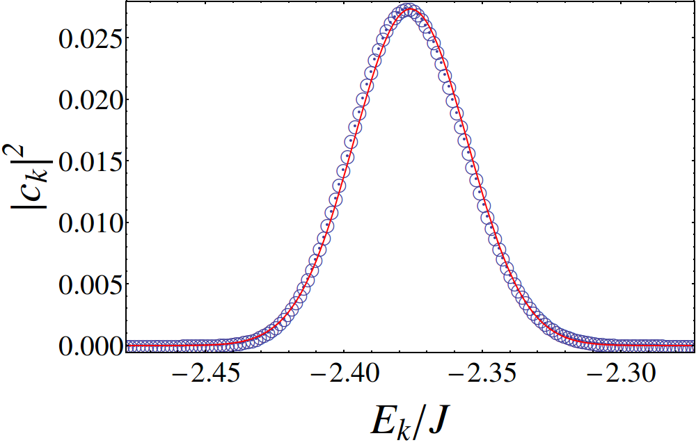
In figure 1 (a), we show the absolute squared components $|c_{k}|^{2}$ as a function of the eigenvalues of the LMG model. The components are very well approximated by a Gaussian function

$$|c_{k}|^{2}\approx g_{k}\equiv Ae^{-\frac{(E_{k}-\bar{E})^{2}}{2\sigma^{2}}},$$ (7)

as depicted in the figure with a solid line. From the normalization condition, the amplitude $A$ can be shown to be

$$A=\frac{1}{\sqrt{2\pi}}\frac{\Delta E_{1}}{\sigma},$$ (8)

where

$$\Delta E_{1}=\langle E_{k+1}-E_{k}\rangle$$ (9)

is the mean of the energy differences between consecutive energies of the states that contribute to the evolution of the coherent state. Concretely, we consider energy states in the interval $[\bar{E}-3.5\sigma,\bar{E}+3.5\sigma]$, where lies $99.95\%$ of the norm of the initial state.

The infinite-time average of the survival probability is therefore given by

$$IPR=\displaystyle\sum_{k}|c_{k}|^{4}\approx A^{2}\displaystyle\sum_{k}e^{-\frac{(E_{k}-\bar{E})^{2}}{\sigma^{2}}}\approx\dfrac{A^{2}}{\Delta E_{1}}\displaystyle\int e^{-\frac{(E-\bar{E})^{2}}{\sigma^{2}}}dE=\dfrac{1}{2\sqrt{\pi}}\dfrac{\Delta E_{1}}{\sigma}.$$ (10)

As discussed in Schliemann2015 (see also A), the standard deviation of the energy distribution of coherent states is $\sigma\propto\sqrt{J}$. With this and from the fact that $\Delta E_{1}$ tends to a finite value in the limit $J\rightarrow\infty$ [see (19) below], expression (10) explains the results of Bastarrachea2016a ; BastarracheaPS2017 , where it was shown that the $IPR$ of coherent states in regular regions scales as $1/\sqrt{J}$ for large $J$.

(a)	(b)
(c)

Figure 1: (a) Absolute squared components (circles) of the chosen coherent state in the energy eigenbasis of the LMG model and its Gaussian approximation using $\Delta E_{1}\approx\omega_{1}$ (solid line). (b) Eigenvalues (circles) in the interval $[\bar{E}-3.5\sigma,\bar{E}+3.5]$ plotted against their ordering numbers in this region. The quadratic fit (11) is shown with a solid line. The inset displays the energy differences of consecutive eigenenergies and their fit. (c) Mean value $\Delta E_{1}$ (red line increasing for small $J$) of the differences of consecutive eigenergies in the same interval as the main panel in (b), $\omega_{max}^{(1)}=E_{kmax+1}-E_{kmax}$ (dark purple line fluctuating in its decay), and $\omega_{1}$ evaluated from (14) (light orange line). The asymptotic value of the three lines, which is the frequency of the classical model $\omega_{cl}=2.818$, is indicated on the right. The inset shows the anharmonicity $e_{2}$ as a function of $J$ calculated numerically from (20) (circles) and from the quadratic fit (triangles). The solid line is the semi-classical approximation in (21). Parameters: $j_{zo}=-\cos(\pi/3)$, $\phi_{o}=\pi/2$, $\bar{E}/J=-2.376$; in (a) and (b): $J=2000$.

III.2 Frequencies and their Distribution

In search of an analytical expression for $SP(t)$, we now concentrate on the two key elements of $SP_{p}(t)$ in (5), namely the frequencies $\omega_{k}^{(p)}$ and their distribution given by the product $|c_{k+p}|^{2}|c_{k}|^{2}$, starting with the first ones.

III.2.1 Frequencies $\omega_{k}^{(p)}$

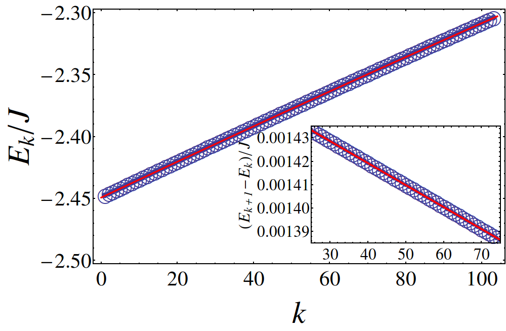
In figure 1 (b), the LMG eigenergies in the interval $[\bar{E}-3.5\sigma,\bar{E}+3.5\sigma]\sim[-2.448J,-2.304J]$ are plotted with blue circles against their ordering numbers in this region. We show with a solid line that the data can be very well fitted with the semi-classical expansion (see B for a detailed derivation)

$$E_{k}=e_{o}+e_{1}k+e_{2}k^{2},$$ (11)

where $k$ is an integer number. This leads to

$$\omega_{k}^{(p)}=(E_{k+p}-E_{k})=p(e_{1}+p\,e_{2})+2\,e_{2}\,p\,k.$$ (12)

The anharmonicity $e_{2}$ measures the departure from a spectrum with equally spaced energies. It is very small, $e_{2}=-0.00094$, when compared with $e_{0}=-4898.46$ and $e_{1}=2.91$. The inset of figure 1 (b) shows the energy differences of consecutive eigenenergies (circles) and the result for $E_{k+1}-E_{k}=(e_{1}+e_{2})+2e_{2}k$ (line), whose slope is given by $e_{2}$. Despite small, $e_{2}$ has an important role in the decay of the survival probability, as will become clear later. Equation (11) is a valid assumption for any coherent state in the semi-classical limit, provided the energy interval defined by its mean energy and width does not include critical energies.

III.2.2 Product $|c_{k+p}|^{2}|c_{k}|^{2}$

Following (7), $|c_{k+p}|^{2}|c_{k}|^{2}\approx g_{k+p}\,g_{k}$. C shows that this product can be very well approximated by a Gaussian distribution for frequencies $\omega_{k}^{(p)}$

$$g_{k+p}\,g_{k}\approx A_{p}\exp\left[-\frac{\left(\omega_{k}^{(p)}-\omega_{p}\right)^{2}}{2\sigma_{p}^{2}}\right],$$ (13)

where the centroid ($\omega_{p}$), amplitude ($A_{p}$), and width ($\sigma_{p}$) are given in terms of the values for $p=1$

$$\omega_{p}\approx p\,\omega_{1}, \hskip 25.6073pt\omega_{1}\approx\sqrt{e_{1}^{2}+4e_{2}(\bar{E}-e_{0})},$$ (14)

$$\frac{A_{p}}{A^{2}}\approx\left(\frac{A_{1}}{A^{2}}\right)^{p^{2}}, \hskip 25.6073pt\frac{A_{1}}{A^{2}}=\exp\left(-\frac{\omega_{1}^{2}}{4\sigma^{2}}\right),$$ (15)

$$\sigma_{p}\approx p\,\sigma_{1}, \hskip 25.6073pt\sigma_{1}=\sqrt{2}\,|e_{2}|\frac{\sigma}{\omega_{1}}.$$ (16)

Therefore, the dominant frequency of the $p$-th component of the survival probability is approximately a harmonic frequency, $\omega_{1}$ being the fundamental one. The value $\omega_{1}$ is where the product of Gaussians $g_{k+1}g_{k}$ takes its maximal value. It is approximately given by the pair of consecutive eigenenergies located around $\bar{E}$

$$\omega_{max}^{(1)}=E_{kmax+1}-E_{kmax},$$ (17)

where the pair $E_{kmax}$ and $E_{kmax+1}$ is defined through the condition $E_{kmax}\leq\bar{E}\leq E_{kmax+1}$.

To determine $A_{1}$, in addition to $\omega_{1}$, we also need $\Delta E_{1}$ through $A$ from (8). Since $\Delta E_{1}$ is the mean value of the differences of consecutive energies in an interval around $\bar{E}$ and these differences vary linearly in this interval [cf. the inset of figure 1 (b)], we can approximate $\Delta E_{1}$ by the energy difference in the center of the interval,

$$\Delta E_{1}\approx\omega_{max}^{(1)}\approx\omega_{1}.$$ (18)

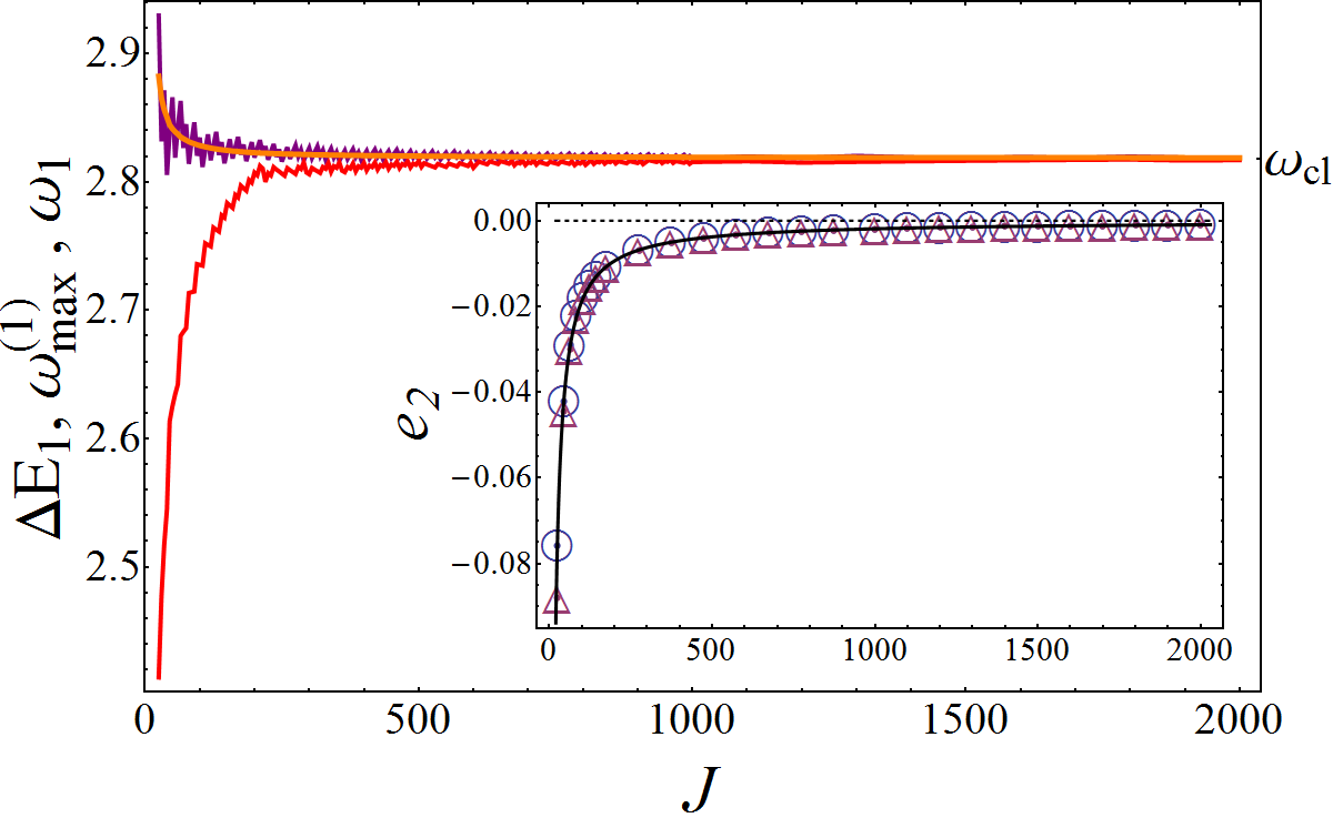
This assumption is not exact, but the three quantities converge, in the limit $J\to\infty$, to the classical frequency $\omega_{cl}$

$$\lim_{J\rightarrow\infty}\Delta E_{1}=\lim_{J\to\infty}\omega_{max}^{(1)}=\lim_{J\to\infty}\omega_{1}=\omega_{cl},$$ (19)

as shown in figure 1 (c) and discussed in B.

It remains to find the width $\sigma_{1}$ in (16), and for this we need $e_{2}$. The anharmonicity is estimated using assumption (11),

$$e_{2}=\frac{E_{kmax+1}+E_{kmax-1}}{2}-E_{kmax}.$$ (20)

Small differences exist between $e_{2}$ estimated with the expression above and the anharmonicity obtained by fitting the spectrum with (11), but both values go to zero as $J$ increases and converge to the semi-classical (see B) expression

$$\lim_{J\rightarrow\infty}e_{2}=\frac{\omega_{cl}}{2J}\frac{d\omega_{cl}}{d\epsilon}\equiv f_{e}/J\ \ \ \ \ \ \ {\hbox{(with \ \ $\epsilon=E/J$)}},$$ (21)

as seen in the inset of figure 1 (c).

III.3 Analytical Expression

Putting the above results together in (5), we have

$$SP_{p}(t)\approx\frac{\omega_{1}^{2}}{\pi\sigma^{2}}\exp\left(-\frac{p^{2}\omega_{1}^{2}}{4\sigma^{2}}\right)\sum_{k}\exp\left[{-\frac{\left(\omega_{k}^{(p)}-p\omega_{1}\right)^{2}}{2p^{2}\sigma_{1}^{2}}}\right]\cos(\omega_{k}^{(p)}t).$$ (22)

Approximating the sum above by an integral (see D for details), we arrive at

$$SP_{p}(t)\approx\frac{\omega_{1}}{\sigma\sqrt{\pi}}\exp\left[-p^{2}\left(\frac{\omega_{1}^{2}}{4\sigma^{2}}+\frac{t^{2}}{t_{D}^{2}}\right)\right]\cos(p\omega_{1}t),$$ (23)

where we define the decay time

$$t_{D}\equiv\frac{\omega_{1}}{\sigma|e_{2}|}.$$ (24)

Expression (23) is valid up to the time when the discrete nature of the spectrum, neglected with the use of the integral, finally manifests itself and induces fluctuations of the survival probability around its asymptotic value.

With the expressions (23) and (10), the equation for the survival probability in (4) becomes,

$$SP(t)\approx\frac{\omega_{1}}{2\sigma\sqrt{\pi}}\left\{1+2\displaystyle\sum_{p=1}\exp\left[-p^{2}\left(\frac{\omega_{1}^{2}}{4\sigma^{2}}+\frac{t^{2}}{t_{D}^{2}}\right)\right]\cos(p\omega_{1}t)\right\},$$ (25)

which is one of the main results of this paper. Equation (25) can also be expressed as a convergent series in terms of the Jacobi theta function  Jacobi , $\Theta_{3}(x,y)=1+2\sum_{p=1}y^{p^{2}}\cos(2px)$, using $x=\omega_{1}t/2$ and $y=\exp\left(-\frac{\omega_{1}^{2}}{4\sigma^{2}}-\frac{t^{2}}{t_{D}^{2}}\right)$,

$$SP(t)\approx\frac{\omega_{1}}{2\sigma\sqrt{\pi}}\Theta_{3}(x,y).$$ (26)

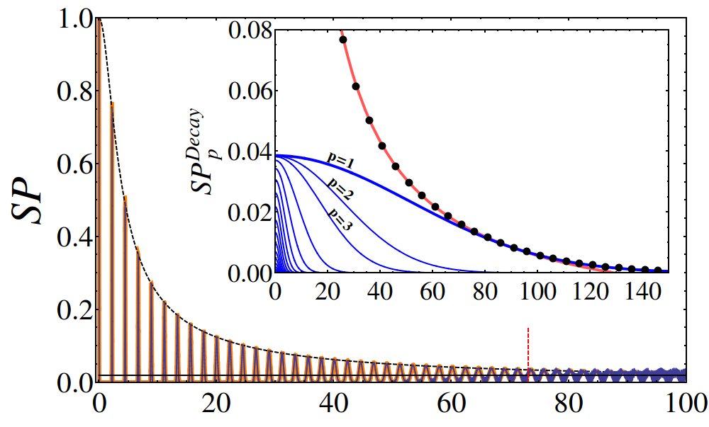
As one sees from (23), the amplitude of each component $SP_{p}(t)$ scales exponentially with $-p^{2}$. Every $SP_{p}(t)$ is an oscillating function with frequency $p\,\omega_{1}$ modulated in time by a Gaussian function

$$SP_{p}^{Decay}(t)=\frac{\omega_{1}}{\sigma\sqrt{\pi}}\exp\left[-p^{2}\left(\frac{\omega_{1}^{2}}{4\sigma^{2}}+\frac{t^{2}}{t_{D}^{2}}\right)\right]$$ (27)

with decay time $t_{D}^{(p)}=t_{D}/p$. The decay of the oscillations of the survival probability in (25) is controlled by the sum of these Gaussians, $SP^{Decay}(t)=IPR+\sum_{p\geq 1}SP^{Decay}_{p}(t)$.

(a)
(b)

Figure 2: (a) Survival probability for the same coherent state as in figure 1 obtained numerically (dark blue line) and using the analytical result (light orange line) in (25). The curves are almost indistinguishable up to $t_{D}$ (vertical dashed line). The dashed line depicts the analytical decay of the oscillations. The inset shows the decay of the different $p$-components ($p>0$, bottom curves), their sum (black dots), and the power law fitting $(2.506/t)-IPR$ (solid red line). (b) is similar to (a), but for longer times. The horizontal black line is the $IPR$.

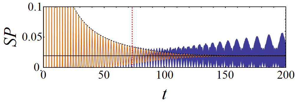In the inset of figure 2 (a), we show the contribution from each $SP_{p}^{Decay}(t)$. The components with large $p$ decay faster than those with small $p$. At long times, the sum of Gaussians is dominated by the $p=1$ component. Therefore, the decay time of $SP_{1}(t)$ is also the decay time of the entire $SP(t)$ and is given by $t_{D}$ from (24). The larger the anharmonicity is, the shorter the decay time becomes, that is faster equilibration. The semi-classical approximation for $t_{D}$ is obtained from (19) and (21) as $t_{D}=2J/(\sigma|d\omega_{cl}/d\epsilon|)$.

We emphasize that in this one-degree of freedom case, only three parameters are needed to fully describe the survival probability at any time up to the equilibration time. As seen from (25), they are the energy width $\sigma$ which can be calculated analytically (see A), the mean energy separation between eigenenergies $\omega_{1}$ (approximated by $\omega_{cl}$ in the semi-classical limit), and the anharmonicity in the energy spectrum $e_{2}$ [with semi-classical limit in (21)]. These parameters depend on the initial state, and we have tested the ability of our analytical expression (25) to describe the numerical $SP$ for many different states, founding a remarkable agreement (as in the case shown below), provided the initial state is far from critical energies.

In E, we show the dependence of $\sigma$, $\omega_{1}$, $e_{2}$ and the decay time (24) on the coordinates of the initial coherent state. Likewise, the small regions in the coherent parameter space close to the critical energies where our approach fails, are identified for the considered case with $J=2000$.

III.4 Comparison with Numerics

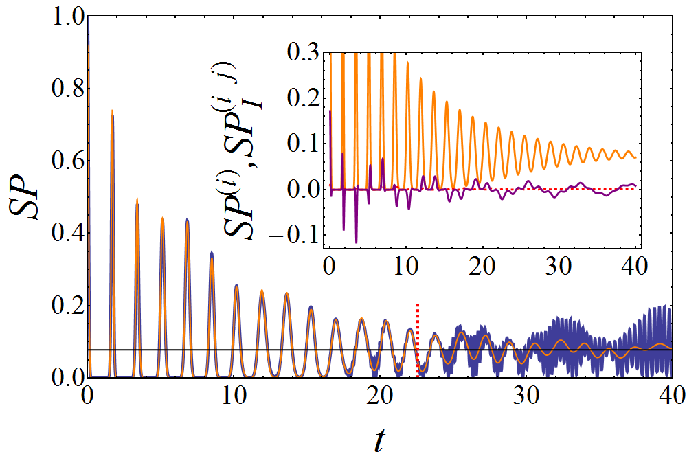
In the main panels of figure 2, we compare the analytical expression (25) and the numerical results for the LMG model using the same parameters and initial state as in figure 1. The relevant parameters obtained with (7) [or (35)], (17), and (20) are $(\sigma,\omega_{1},e_{2})=(41.08,2.82,-9.38\times 10^{-4})$, which gives the decay time $t_{D}=73.09$.

The analytical approximation reproduces remarkably well the numerical results up to $t_{D}$. The two lines in the main panel of figure 2 (a) can hardly be distinguished. The numerical oscillations as well as their decay agree extremely well with the analytical expression (25).

At times of the order of $t_{D}$, the decay of the oscillations of the survival probability is power law, in accord with Santos2016 . This is confirmed with the fit $2.506/t$ illustrated with a solid red line in the inset of figure 2 (a). This behavior, including the pre-factor, can be justified analytically in the semi-classical limit (see the next subsection and F ).

Figure 2 (b) makes more evident what happens at long times, when the discrete nature of the spectrum becomes important. Beyond $t_{D}$, the numerical curve fluctuates around the infinite time average, while the analytical expression simply stabilizes at $IPR$.

III.5 Classical Limit

The analytical expression (25) for the survival probability has a well defined classical limit. In this limit, $e_{2}\approx f_{e}/J$ [see (21)] goes to zero faster than the growth of $\sigma\approx f_{\sigma}\sqrt{J}$ [see (36)]. Consequently, the decay time goes to infinity,

$$\lim_{J\rightarrow\infty}t_{D}=\lim_{J\rightarrow\infty}\frac{\omega_{1}}{\sigma|e_{2}|}\propto\lim_{J\to\infty}\sqrt{J}=\infty,$$ (28)

and the expression (25) for the $SP$ becomes a sum of Kronecker deltas (see F)

$$\lim_{J\rightarrow\infty}SP(t)=\sum_{n\in\mathbb{Z}}\delta_{t,n\tau}f_{n},$$ (29)

with $\tau=2\pi/\omega_{cl}$ and $f_{n}=(1+(4\pi f_{\sigma}^{2}f_{e}/\omega_{cl}^{3})^{2}n^{2})^{-1/2}$. This result indicates periodic instantaneous revivals, which are indeed expected for the survival probability in a one-degree of freedom, regular classical system.

	(a)	(b)	(c)
$|c_{k}|^{2}$
	(d)	(e)	(f)
	$E_{k}/J$	$E_{k}/J$	$E_{k}/J$

Figure 3: Eigenenergy components of a sample of coherent states with the same mean energy ($E/J=-1.8$) for the Dicke model with $\omega=\omega_{0}=\gamma=1$ and $J=120$. The Bloch coherent parameters are $\phi_{o}=0$ and $j_{z}=-0.505$ (a), $-0.452$ (b), $-0.116$ (c), $0.019$ (d), $0.113$ (e), $0.140$ (f), and the Glauber parameters are $p_{o}=0$ and $q_{o}$ given by the condition $\langle\alpha_{o}z_{o}|H_{D}|\alpha_{o}z_{o}\rangle/J=-1.8$. Solid lines in panels (a), (b) and (f) represent Gaussian fits (parameters in table 1) for the sub-sequences with the largest components $|c_{k}|^{2}$. Vertical dashed lines in panels (a), (b) and (f) indicate the sample of energy components used in figures 5(a) and 6.

With the asymptotic expressions for $\sigma$, $\omega_{1}$ and $e_{2}$, it is possible to justify the power law observed in figure 2 for the decay of the survival probability at times of the order $t_{D}$. For this, we investigate $SP^{Decay}(t)$, that is, (25) without the cosine function. F shows that for large $J$, $SP^{Decay}\approx c/t$, where $c$ is an asymptotically finite value given by $c=\frac{\omega_{cl}^{2}}{2\sigma^{2}|e_{2}|}$. For the parameters used in figure 2, we find $c=2.512$, which is in excellent agreement with the fit in the inset of figure 2 (a), which gives $c=2.506$.

IV Survival probability in two-degree-of-freedom models

We now use the Dicke model in the superradiant phase to characterize the dynamics of quantum models with two-degrees of freedom. The Dicke model has both regular and chaotic regimes. The classical regular dynamics occurs at low energies Bastarrachea14PRA-2 ; Chavez2016 and is accounted for by quasi-integrals of motion Relano16 ; BastaJPA17 .

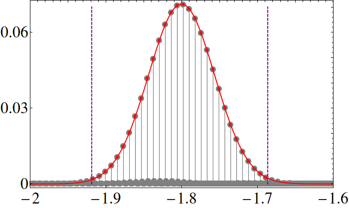
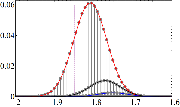
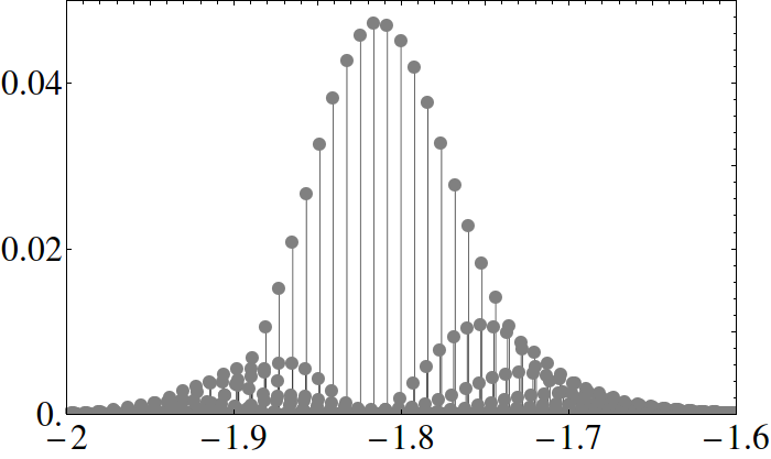
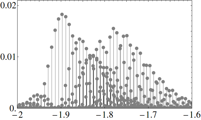
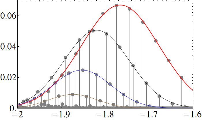
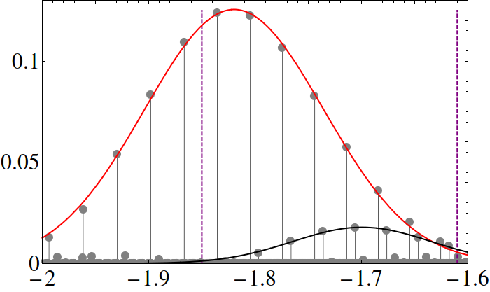
The description of the evolution of the survival probability for the Dicke model is richer than what we can find in models with one-degree of freedom. This happens because, in general, the projection of coherent states into the energy eigenbasis no longer leads to a single sequence of components $|c_{k}|^{2}$ following a single Gaussian function, as for the LMG model in figure 1 (a). Instead, the components of the initial state now form different sub-sequences (figure  3). In the regular regime, these sub-sequences are overall still represented by Gaussian functions, but of different means and widths. These various sub-sequences interfere and lead to a more complex behavior of the survival probability. The energy eigenbasis decomposition of the coherent states is closely related with the properties of the classical phase space of the Dicke model, as it will be shown below.

After a discussion in subsection IV.1 about the different energy distributions of the coherent states displayed in figure 3, we select four representative cases and analyze their survival probability in the following subsections. We start in Sec. IV.2 with the state in figure 3 (a). This initial state activates only one of the degree of freedom, and, as a consequence, the analytical expression of the previous section describes very well the numerical results. In section IV.3, we consider the states from figures 3 (b) and (f). They are representative cases of initial states activating simultaneously the two-degrees of freedom, which yields to interference terms that we are able to describe analytically with formula (34). For Sec. IV.4, we choose the state from figure 3 (d) to illustrate the effects of the non-linear instabilities and unveil the signature of classical chaos in the quantum dynamics. The selected initial states are representative of the whole cases that can be found in the regular regime of the Dicke model. In LermaAIP18 other coherent states at the same and also larger energies than the one used here, are studied, reinforcing the validity of the results presented and discussed below.

IV.1 Initial coherent states

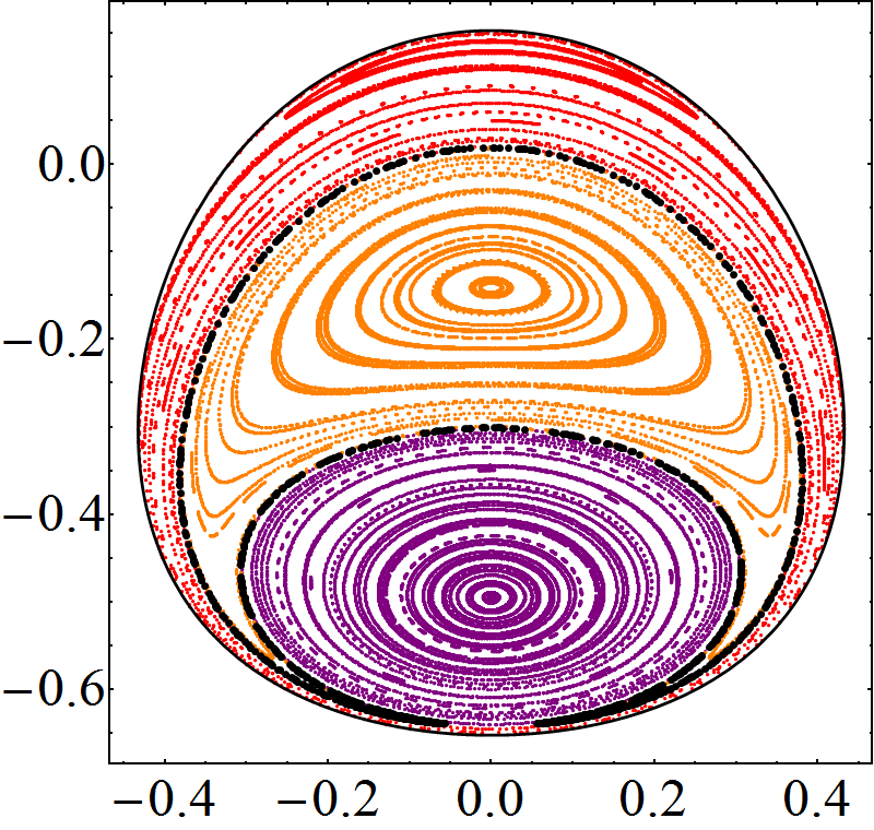
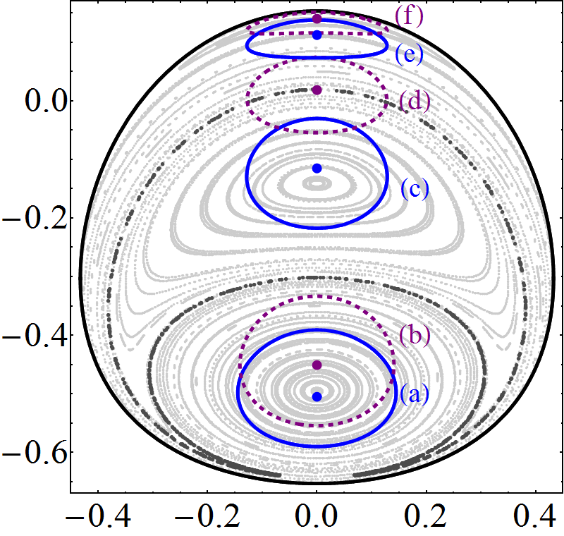
In figure 3, we fix $\phi=0$ and $p=0$, vary $j_{z}$, and determine $q$ from the condition that guarantees that all chosen coherent states have the same mean energy $E/J=-1.8$, which is relatively close to the ground-state ($E_{GS}/J=-2.125$). Regular dynamics dominates this energy region, as seen in figure 4 (a). This figure shows Poincaré sections for the classical limit of the Dicke model at $E/J=-1.8$. The closed loops, covering the whole Poincaré surface, reflect the existence of invariant tori. Their nature can be revealed in light of the adiabatic approximation Relano16 ; BastaJPA17 : for the parameters ($\omega=\omega_{0}=\gamma=1$) and energy chosen here, the dynamics of the bosonic variables $(p,q)$ is slower than that of the pseudospin variables. The pseudospin precesses rapidly around a slowly changing $q$-dependent axis. The nearly constant angle $\beta$ that forms the pseudospin with respect to the precession axis defines an effective one-dimensional adiabatic potential for the bosonic variables. If the angle $\beta$ is small, the amplitude of the bosonic variables is large and vice-versa.

The Poincaré sections in figure 4 (a) can then be understood as follows:

• The trajectories rotating around $(j_{z},\phi)\approx(-0.5,0)$ (plotted in purple) correspond to small precessing angles $\beta$ and wide amplitudes of the bosonic excitations.

• The trajectories rotating around $(j_{z},\phi)\approx(0.15,0)$ (plotted in red) have large $\beta$ and consequently small displacements of the bosonic variables.

• The trajectories in the center (plotted in orange), rotating around the point $(j_{z},\phi)\approx(-0.15,0)$, indicate the breaking of the adiabatic approximation. They emerge from nonlinear resonances between the adiabatic modes. These trajectories are the precursors of ample chaotic regions that appear for energies larger than the one considered here. In fact, a detailed view of the separatrix between this last set of trajectories and the two former ones reveals the existence of a narrow region with classical chaotic trajectories BastarracheaPS2017 .

The six coherent states of figure 3 sample the three classical regions listed above. In figure 4 (b), we show where these states fall in the Poincaré surface. Each point in figure 4 (b) indicates the phase-space coordinates associated with the coherent state parameters ($z_{o},\alpha_{o}$), and the curve surrounding each point represents the spreading of the corresponding coherent state wave function in phase space (level curves $|\langle z,\alpha|z_{o},\alpha_{o}\rangle|^{2}=e^{-1}$ for $J=120$).

	(a)	(b)
$j_{z}$
	$\phi$	$\phi$

Figure 4: (a) Poincaré sections ($p=0$) projected in the plane $j_{z}-\phi$ for the classical Dicke model with the same parameters and energy as figure 3. The dark black trajectory indicates the separatrix between the region of nonlinear resonances (central light orange trajectories) and the regions of the adiabatic modes (outer light red trajectories for the pseudospin and dark purple for the bosonic mode). (b) Location of the coherent states from figure 3 in the classical phase space. Dots (from bottom to top) indicate the coherent states from figure 3 (a) to figure 3 (f). The closed curves that encircle the dots represent the spreading of the corresponding wave functions (level curves $|\langle z,\alpha|z_{o},\alpha_{o}\rangle|^{2}=e^{-1}$) for $J=120$.

According to the list above, the states in figures. 3 (a) and (b) are associated with large bosonic amplitudes and those in figures. 3 (e) and (f) with large pseudospin precession angles. They have one sequence (a) or sub-sequences (b, e, f) of components described by Gaussian distributions. The differences of consecutive energies in the sub-sequences of figures. 3 (e) and (f) are larger than in figures. 3 (a) and (b). This can be qualitatively understood from the classical model, because the pseudospin has faster dynamics than the bosonic variables, and thus larger oscillation frequencies.

The state in figure 3 (a) is representative of nearly pure bosonic excitations. Its components $|c_{k}|^{2}$ are well approximated by a single Gaussian function. This situation is equivalent to what we have for the LMG model, so the analytical expression (25) is still applicable here. This state corresponds classically to pseudospin precessing angle $\beta=0$ and maximal amplitude of the bosonic variables.

In contrast, the state in figure 3 (f) is representative of nearly pure pseudospin excitations. Its components $|c_{k}|^{2}$ are well described by a dominant Gaussian distribution with a second smaller Gaussian sub-sequence. In the classical picture, this state corresponds to nearly maximal precessing pseudospin angle and nearly zero amplitude of the bosonic variables.

The states in figures. 3 (b) and (e) have more than a single sequence of components; three Gaussians are identifiable in (b), while four are distinguished in (e). The presence of several sub-sequences of components in these states corresponds classically to the simultaneous excitation of different adiabatic modes, with the dominance of one of them, the bosonic one in figure 3 (b) and the pseudospin mode in figure 3 (e).

The state in figure 3 (c), located close to the center of the region of nonlinear resonances, exhibits a dominant Gaussian sub-sequence and many smaller ones, while the coherent state in figure 3 (d) has a complicated structure with so many eigenstates participating that it is hard to identify the sub-sequences (if any). In the classical phase space of figure 4 (b), this state is located in the unstable separatrix between the region of non-linear resonances and the fast mode of the adiabatic approximation, where, as it is known ReichlBook , classical chaos emerges.

IV.2 One-sequence coherent state

(a)	(b)
(c)
$t$

Figure 5: (a) Energies (dots) of the 30 largest components of the coherent state of figure 3 (a) (the ones located between the two vertical dashed lines in that figure). The solid line is a fit using (11). The inset shows the difference between consecutive energies and the corresponding fit. (c) Survival probability for the coherent state of figure 3 (a): numerical curve (dark blue) and analytical expression (light orange). The inset shows the same figure in log-log scale. (b) Closer view around the decay time $t_{D}$. In both panels, the dashed black line depicts the analytical decay of the oscillations of $SP$. The vertical dashed line indicates the decay time $t_{D}=451.5$ and the horizontal solid black line is the $IPR=0.0496$.

In figure 3 (a), we show a Gaussian fit to the energy components of the coherent state. The mean and the width $\sigma$ obtained from the fitting match those calculated analytically through the expectation values $\langle H_{D}\rangle$ and $\langle H_{D}^{2}\rangle$ (see A). This agreement confirms that this state is indeed very well described by a single sequence of energy components.

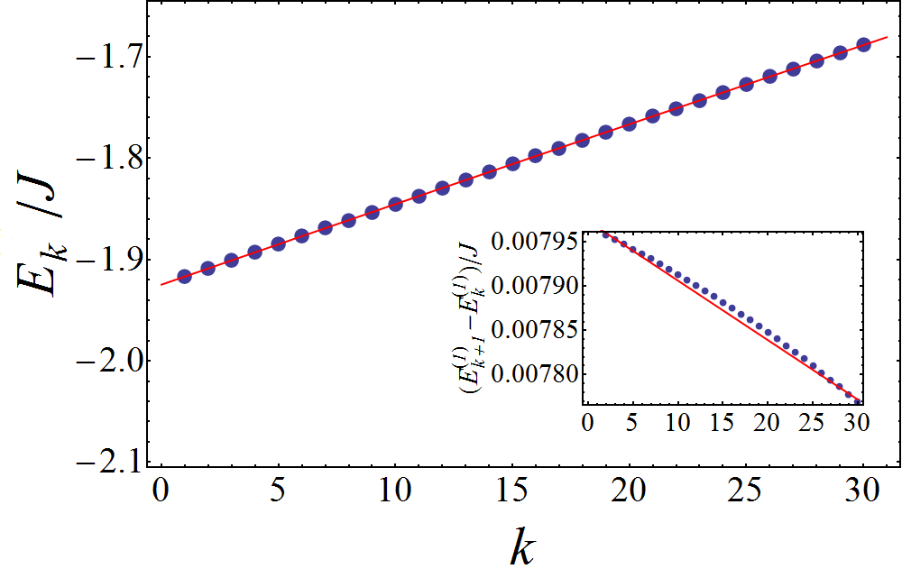
The energy levels $\{E_{k}\}$ that are relevant to the evolution of the coherent state, i.e. those with non-negligible $|c_{k}|^{2}$, are very well described by the semi-classical approximation (11), as can be seen in figure 5 (a). A tiny discrepancy is visible by plotting the energy difference $E_{k+1}-E_{k}$ in the inset of figure 5 (a), which could be related with the small $J$ accessible to our numerical analysis of the Dicke model ($J=120$). However, as we show below, (11) can still be successfully employed for the description of the survival probability.

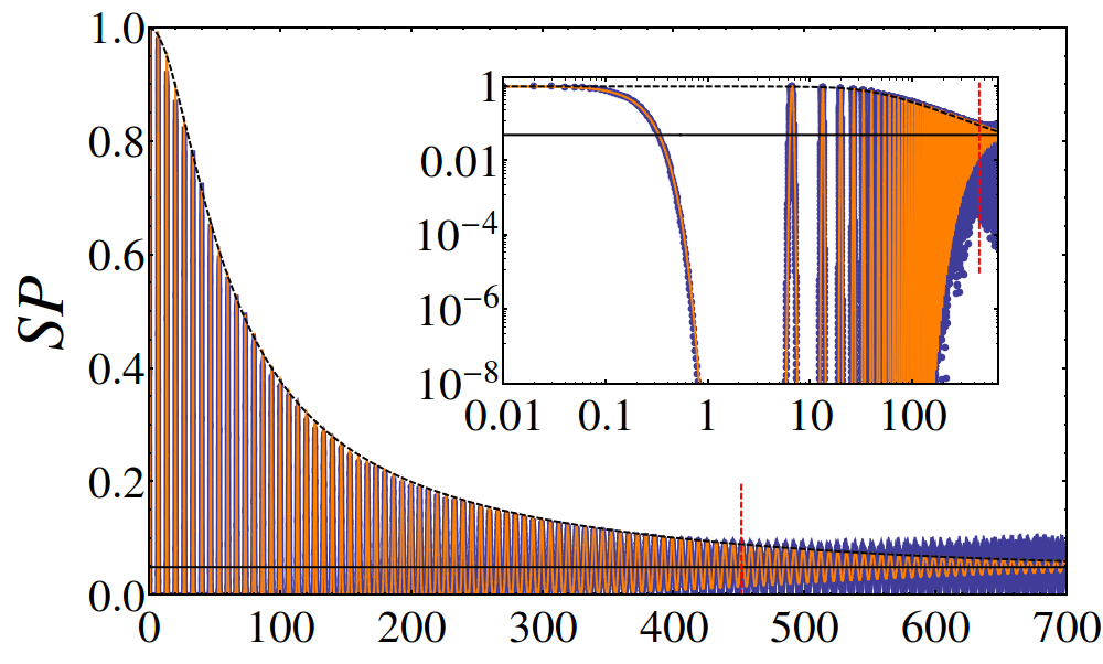
The analytical expression (25) used for the LMG model can be used here also. Using (17) and (20) in the numerically evaluated spectrum, we obtain $(\omega_{1},e_{2})=(0.9456,-0.399\times 10^{-3})$, which together with the calculated width $\sigma/J=0.0436$ give the decay time $t_{D}=451.5$.

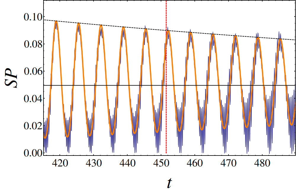
The analytical approximation (25) and the numerical results for the survival probability are compared in figures. 5 (b) and (c) both in linear (main panels) and log-log (inset) scales. The analytical approximation gives a very accurate description of $SP(t)$ from $t=0$ until $t_{D}$. Beyond the equilibration time, the discreteness of the energy spectrum becomes relevant. It leads to small fluctuations that are not captured by the analytical expression, as seen in figure 5 (b).

IV.3 Interference terms

When the components of the initial state can be fitted with more than a single Gaussian, as in figure 3 (b) and figure 3 (f), we use the index $i$ to denote the components $|c_{k}^{(i)}|^{2}$, energies $\{E_{k}^{(i)}\}$, and the Gaussian curve $g_{k}^{(i)}=A_{i}e^{-(E_{k}^{(i)}-\bar{E}_{i})/(2\sigma_{i}^{2})}$ associated with each sub-sequence. Three Gaussians ($i=1,2,3$) are used for the state in figure 3 (b) and two ($i=1,2$) for the state in figure 3 (f). In these cases, (4) for the survival probability can be written as

$$SP(t)=\left|\sum_{ik}|c_{k}^{(i)}|^{2}e^{-iE_{k}^{(i)}t}\right|^{2}=\sum_{i}SP^{(i)}(t)+\sum_{i<j}SP_{I}^{(ij)}(t).$$ (30)

The novelty with respect to (25) is the interference terms $SP_{I}^{(ij)}$. The steps involved in the derivation of the terms $SP^{(i)}$ are similar to those taken in Sec. III and an equation equivalent to (26) is obtained

$$SP^{(i)}(t)=\frac{A_{i}^{2}\sigma_{i}\sqrt{\pi}}{\omega_{1}^{(i)}}\Theta_{3}(x_{i},y_{i}),$$ (31)

with $x_{i}=\omega_{1}^{(i)}t/2$ and $y_{i}=e^{-\left(\omega_{1}^{(i)}/2\sigma_{i}\right)^{2}}e^{-\left(t/t_{D}^{(i)}\right)^{2}}$. Analogously to Sec. III, the decay time of each isolated sub-sequence is $t_{D}^{(i)}=\omega_{1}^{(i)}/(|e_{2}^{(i)}|\sigma_{i})$; the frequency $\omega_{1}^{(i)}=E_{kmax+1}^{(i)}-E_{kmax}^{(i)}$ is the difference of the closest energies of the $i$-th sub-sequence to the mean energy $\bar{E}_{i}$, with $E_{kmax}^{(i)}\leq\bar{E}_{i}\leq E_{kmax+1}^{(i)}$; and the anharmonicity is $e_{2}^{(i)}=(E_{kmax+1}^{(i)}+E_{kmax-1}^{(i)})/2-E_{kmax}^{(i)}$.

(a)	(b)

Figure 6: (a) Energies of the largest components of the three sub-sequences contributing to the coherent state in figure 3 (b). The sampled energies are the ones located between the two vertical dashed lines in that figure. Each sub-sequence has a different color, which corresponds with the colors used in figure 3 (b) . The inset shows the energy differences between two distinct sub-sequences (dots) and the respective mean values (horizontal lines). (b) Similar to panel (a), but for the largest components of the two principal sub-sequences of the coherent state in figure 3 (f).

To obtain an analytical expression for $SP_{I}^{(ij)}$, we use the same strategy used in Sec. III, namely we separate the terms according to the index distance $p$ between the eigenvalues

$$SP_{I}^{(ij)}(t)=2\displaystyle\sum_{p\in\mathbb{Z}}\sum_{k}|c_{k}^{(i)}|^{2}|c_{k+p}^{(j)}|^{2}\cos\left[(E_{k+p}^{(j)}-E_{k}^{(i)})t\right].$$ (32)

In addition, we assume that the energy sub-sequences are of the form (11) and related by a constant shift $\delta E_{ij}$

$$\delta E_{ij}=E_{k}^{(i)}-E_{k}^{(j)}.$$ (33)

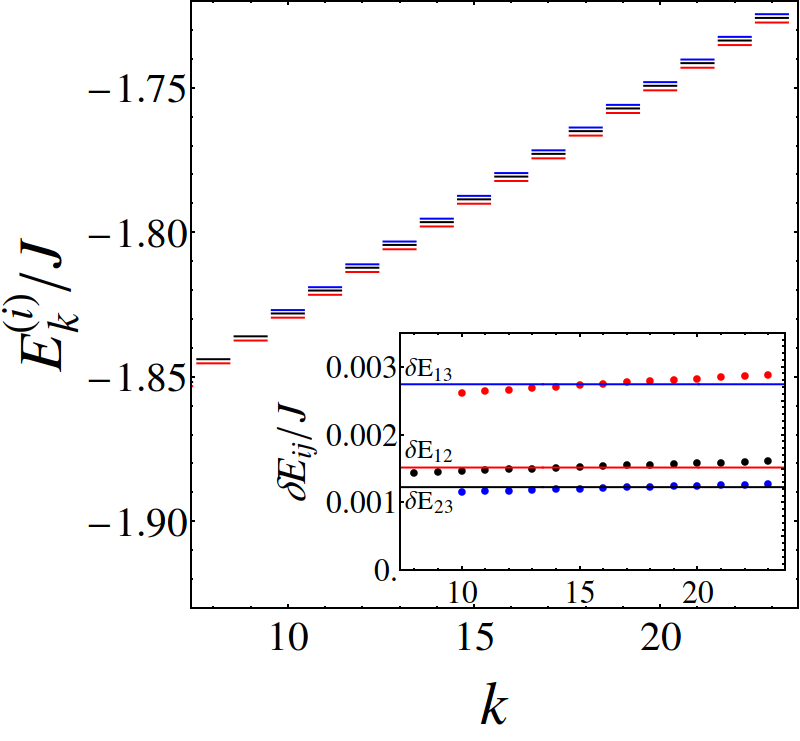
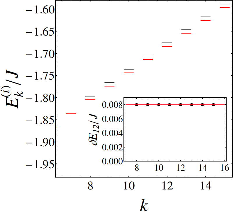
This is an important step in the derivation of an expression for $SP_{I}^{(ij)}(t)$. In figure 6 (a) and figure 6 (b), we show the energies $\{E_{k}^{(i)}\}$ of each Gaussian sub-sequence of the coherent states from figure 3 (b) and figure 3 (f), respectively. The insets of figure 6 (a) and (b) confirm the validity of (33). The agreement is not perfect, but it should improve for larger $J$.

$i$	$A_{i}$	$\bar{E}_{i}/J$	$\sigma_{i}/J$	$\omega_{1}^{(i)}/J$	$e_{2}^{(i)}/J$	$t_{D}^{(i)}$	$i,j$	$\omega_{ij}/J$	$\delta E_{ij}/J$
Coherent state of figure 3(b)
1	0.0612	-1.809	0.0421	0.00788	$-3.3\times 10^{-6}$	476.80	1,2	0.00786	0.00152
2	0.0105	-1.771	0.0394	0.00786	$-3.7\times 10^{-6}$	447.08	1,3	0.00785	0.00275
3	0.0025	-1.751	0.0382	0.00785	$-4.1\times 10^{-6}$	420.97	2,3	0.00785	0.00123
Coherent state of figure 3(f)
1	0.126	-1.820	0.0841	0.0308	-0.000135	22.57	1,2	0.0303	0.00802
2	0.018	-1.699	0.0667	0.0297	-0.000134	27.73

Table 1: Parameters determined from the numerical spectrum of the coherent states of figure 3 (b) and figure 3 (f), and used in the analytical expression (30) for the survival probability plotted in figures 7 and 8 (a).

From the assumption (33) and using $|c_{k}^{(i)}|^{2}\approx g_{k}^{(i)}$ , the following expression is obtained for the interference terms (see G for a detailed derivation),

$$SP_{I}^{(ij)}(t)=\frac{2A_{i}A_{j}\sqrt{2\pi}\sigma_{i}\sigma_{j}}{\omega_{ij}\sqrt{\sigma_{i}^{2}+\sigma_{j}^{2}}}\displaystyle\sum_{p\in\mathbb{Z}}e^{-\frac{(p\omega_{ij}+\delta E_{ij}+\bar{E}_{i}-\bar{E}_{j})^{2}}{2(\sigma_{i}^{2}+\sigma_{j}^{2})}}e^{-\frac{(\sigma_{ij}pt)^{2}}{2}}\cos[(\delta E_{ij}+p\omega_{ij})t].$$ (34)

Above,

$$\sigma_{ij}=\frac{2|e_{2}^{(i)}|\sigma_{i}\sigma_{j}}{\omega_{ij}\sqrt{\sigma_{i}^{2}+\sigma_{j}^{2}}},$$

and $\omega_{ij}=E_{k_{I}+1}^{(i)}-E_{k_{I}}^{(i)}$ is the energy difference between the eigenvalues of the $i$-th sub-sequence that are closest to the value $E^{(I)}_{ij}$ that maximizes the product of Gaussians $g_{k}^{(i)}g_{k}^{(j)}$. This value is given by

$$E^{(I)}_{ij}=\frac{\bar{E}_{i}\sigma_{j}^{2}+\bar{E}_{j}\sigma_{i}^{2}}{\sigma_{i}^{2}+\sigma_{j}^{2}}$$

and satisfies $E_{k_{I}}^{(i)}\leq E^{(I)}_{ij}\leq E_{k_{I}+1}^{(i)}$.

(a)
(b)

Figure 7: (a) Survival probability for the coherent state in figure 3 (b): numerical curve (dark blue line), analytical approximation from (30) (light orange), and analytical modulation of the revivals (black dashed lines). The inset shows a small time interval of the main panel to emphasize the agreement between the expression and the numerics. (b) Closer view around the decay time $t_{D}^{(1)}$ of the main sub-sequence of participating energy levels. This decay time is indicated with vertical lines in both main panels. The horizontal black line depicts $IPR=0.0365$.

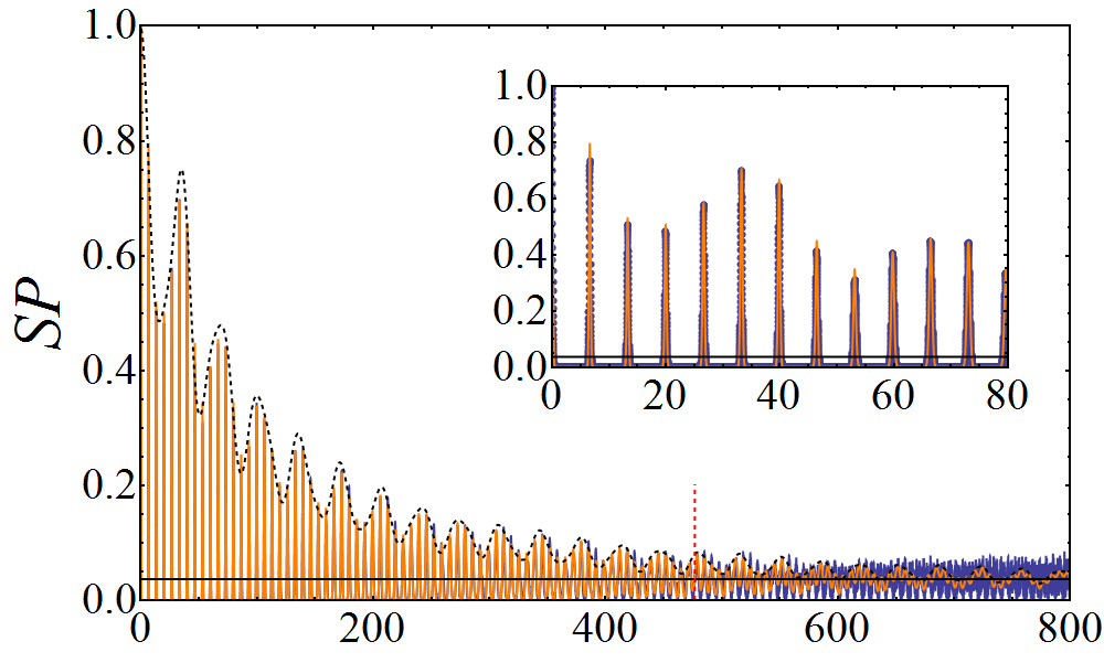
All these contributions are now gathered into (30), which can be compared with the numerical results. At variance with the case of a single sequence, when several sub-sequences participate in the energy eigenbasis decomposition of the coherent states, one needs to deal with several parameters to describe the evolution of the survival probability. Although they can be obtained analytically employing a semi-classical analysis, here we estimate them numerically from the exact energy spectrum.

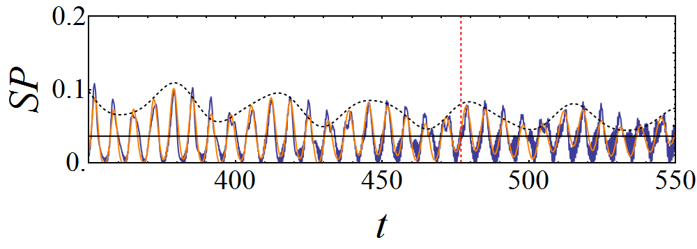
In figure 7, we study the evolution of the survival probability for the coherent state from figure 3 (b). The parameters employed in (30) are shown in table 1. The analytical expression provides an accurate description of the numerical result from $t=0$ until the decay time $t_{D}^{(1)}$ of the dominant sub-sequence. The expression captures the details of the interference terms. They produce slow oscillations that modulate the fast revivals associated with the isolated sub-sequences. These slow oscillations are approximately described by the analytical expression by making $x_{i}=0$ and $p\omega_{ij}=0$ in the arguments of the Jacobi theta and cosine functions in (31) and (34), respectively. The result is shown in both panels of figure 7 with dashed lines. The inset of figure 7 (a), which zooms in a small time interval of the main panel, reinforces the accuracy of the analytical expression.

Analogously to figure 2 (b) in Sec. III, figure 7 (b) makes explicit the effects of the discrete nature of the quantum spectrum, which becomes important for $t>t_{D}^{(1)}$. These effects are neglected by the analytical approximation, whose oscillations beyond the decay time differ from those of the numerics.

(a)	(b)

Figure 8: (a) Survival probability for the coherent state in figure 3 (f): numerical curve (dark blue line) and analytical approximation (light orange). The decay time $t_{D}^{(1)}$ of the dominant sub-sequence is indicated with a dashed vertical line. The horizontal black line depicts $IPR=0.0777$. The inset shows $SP^{(1)}(t)$ (light orange line), $SP^{(2)}(t)$ (red dashed line), and $SP_{I}^{(12)}(t)$ (dark purple line). (b) Numerical result for the survival probability of the coherent state in figure 3 (d), which is located at the separatix between the region of nonlinear resonances and the region of adiabatic modes. The inset shows the evolution in a shorter time interval.The $IPR=0.00855$ is shown by a horizontal black line, but its is so close to the horizontal axis that it is difficult to distinguish it.

In figure 8 (a), expression (30) is compared with the numerical results for the survival probability of the coherent state from figure 3 (f), showing excellent agreement from $t=0$ up to the decay time $t_{D}^{(1)}$. This state has two main sub-sequences, whose adjusted parameters are given in table 1. Notice that the frequency of the revivals is larger than in figure 5 and figure 7. As discussed in IV.1, this can be qualitatively understood because the coherent state from figure 3 (f) is located in a region of the phase space corresponding to wide and fast pseudospin excitations, in contrast with the states of figures 5 and 7, which are dominated by the slow bosonic mode.

On the other hand, the anharmonicities $e_{2}^{(i)}$ of the state of figure 8 (a) are also larger than for the states of figures 5 and 7. This yields a decay time for the survival probability in figure 8 (a) that is one order of magnitude smaller, so fewer revivals are seen before $t_{D}^{(1)}$.

Also in contrast with figure 7 is the almost lack of modulation of the fast oscillations in figure 8 (a). This happens, because the effect of the interference term is less pronounced, as can be confirmed in the inset of figure 8 (a), which shows separate curves for $SP^{(1)}(t)$, $SP^{(2)}(t)$, and $SP_{I}^{(12)}(t)$.

IV.4 Effects of the nonlinear resonances

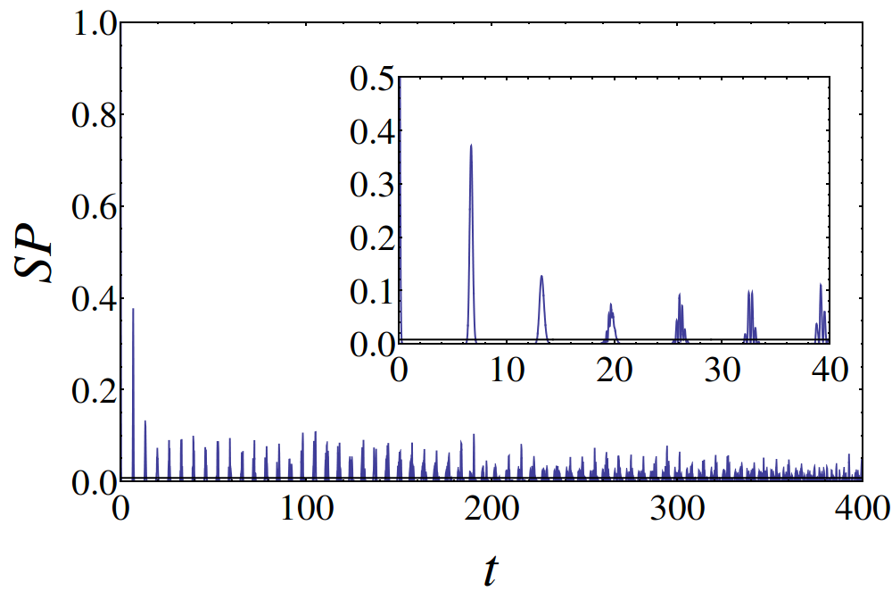
In figure 8 (b), we show the numerical result for the survival probability of the coherent state of figure 3 (d), which is located at the separatrix of the nonlinear resonances region of the classical phase space, where chaos emerges. The eigenstate decomposition of this initial state is complex, with no easily identifiable structures. This is reflected in the rapid decay of $SP(t)$, the weakness of its partial revivals (inset of the same figure), and the fact that the $IPR$ is one order of magnitude smaller than in the previously discussed cases, where analytical approximations were applicable.

The fast decay of the survival probability signals the presence of a narrow chaotic region, which becomes larger for higher energies. The complicated eigenstate decomposition of this initial coherent state is a quantum manifestation of classical nonlinear resonances related to the behavior of the Husimi function of the eigenstates of the standard map reported in Wisniacki2015 .

V Conclusions

We have studied, in the semi-classical limit, the quantum dynamics of bounded systems with one- and two-degrees of freedom represented by the LMG and Dicke Hamiltonians, respectively. For this, we employed the survival probability and used coherent quantum states as initial states. Our focus was on parameters and energies for which both models have classical regular trajectories.

Contrary to a great number of studies of the survival probability that are numerical and concentrate on some intervals of time, we obtained analytical results that cover the entire evolution, from $t=0$ to equilibration. This allowed us to understand the onset of partial revivals, the rate of their decay, and the equilibration time. The characterization of the time scales involved in the relaxation process of isolated quantum systems is a major open question. The fact that we were able to determine the equilibration time analytically is an important contribution to the field.

The analysis presented here is valid in general for bounded models with few degrees of freedom and can be extended to study the dynamical evolution of other observables. For instance, models such as the generalized Dicke Jaako16 and the non-linear Rabi and Dicke models Felicetti15 ; Penna17 are well suited for being studied with our approach.

The initial coherent states are not only experimentally accessible, but they allow for a connection with the classical phase space. Therefore, they are a natural starting point for theoretical and experimental studies of the dynamical consequences of chaos on the survival probabilities and other physical observables.

The evolution of the survival probability depends on the energy distribution of the initial state. For one-degree of freedom systems and for two-degrees of freedom systems when only one of the two degrees of freedom is excited, the spectrum of the energy states contributing to the initial state is quasi-harmonic with Gaussian weights. In this case, an expression for the survival probability in terms of the Jacobi theta function was derived and shown to be in excellent agreement with the numerical results. The expression describes the periodic partial revivals of the initial state and the slow equilibration. We also found that the equilibration time, given by the inverse of the anharmonicity parameter, diverges in the classical limit.

In more complex situations where the two-degrees of freedom are excited, the dynamics is determined by several interference terms that result in the modulation of the revivals. For the regular regime, we were still able to derive an analytical expression. As the system approaches chaotic regions, the distribution of the components of the initial state loses a simple recognizable structure, resulting in very short equilibration times.

An interesting future direction is to connect the results of this work with those of Altland2012NJP , where the temporal evolution of initial coherent states under the Dicke model was also studied. We conjecture that the analytical formula given here is related to the classical drift term in Altland2012NJP , while the fluctuations observed at times longer than the equilibration time are related to a diffusive quantum term.

Appendices

Appendix A Standard deviations of the Hamiltonians in coherent states

The standard deviations of the LMG and Dicke Hamiltonians in coherent states were calculated in Schliemann2015 . Here, we simply correct some misprints found in that reference.

According to equation (69) of Schliemann2015 , and after redefining parameters to be consistent with our parametrization for the LMG model (we have also corrected two misprints in the third and fourth line of Eq.(70) in Schliemann2015 ), the standard deviation of the Hamiltonian in a coherent state is

$$\sigma_{LMG}^{2}=\langle z|H_{LMG}^{2}|z\rangle-\langle z|H_{LMG}|z\rangle^{2}=\Omega_{1}+\Omega_{2}$$ (35)

where (defining $\cos\theta=j_{z}$)

$$\Omega_{1}=\frac{J}{2}\left[-2\gamma_{x}\cos\theta\sin^{2}\theta\cos^{2}\phi-2\gamma_{y}\cos\theta\sin^{2}\theta\sin^{2}\phi\right.$$

$$+\gamma_{x}^{2}(\sin^{4}\theta\cos^{2}\phi\sin^{2}\phi+\cos^{2}\theta\sin^{2}\theta\cos^{2}\phi)+\gamma_{y}^{2}(\sin^{4}\theta\cos^{2}\phi\sin^{2}\phi+\cos^{2}\theta\sin^{2}\theta\sin^{2}\phi)$$

$$\left.+\sin^{2}\theta-2\gamma_{x}\gamma_{y}\sin^{4}\theta\cos^{2}\phi\sin^{2}\phi\right],$$

is of order $J$. In the limit $J>>1$, this is the dominant term of $\sigma_{LMG}$, since

$$\Omega_{2}=\frac{1}{8}\left(1-\frac{1}{2J}\right)\left[-4\gamma_{x}\gamma_{y}\cos^{2}\theta+(\gamma_{x}(1-\sin^{2}\theta\cos^{2}\phi)+\gamma_{y}(1-\sin^{2}\theta\sin^{2}\phi))^{2}\right]$$

is of order $J^{0}$ and $J^{-1}$. From the previous expressions, it is clear that in the limit $J\rightarrow\infty$, the uncertainty of $H_{LMG}$ scales as

$$\sigma_{LMG}\approx f_{\sigma}\sqrt{J}.$$ (36)

Similarly, the uncertainty of the Dicke Hamiltonian in coherent states is depicted by equation (85) of Schliemann2015 . The result in our parametrization (and after correcting a misprint in the third line of equation (86) in Schliemann2015 ) is

$$\sigma_{D}^{2}=\langle z\alpha|H_{D}^{2}|z\alpha\rangle-\langle z\alpha|H_{D}|z\alpha\rangle^{2}=\Omega_{1}+\Omega_{2},$$

where, again, $\Omega_{1}$ is linear in $J$,

$$\Omega_{1}=J\left\{\frac{\omega^{2}}{2}(q^{2}+p^{2})+\frac{\omega_{o}^{2}}{2}\sin^{2}\theta+2\gamma^{2}\left[(\sin^{2}\theta\sin^{2}\phi+\cos^{2}\theta)q^{2}+\sin^{2}\theta\cos^{2}\phi\right]\right.$$

$$+2\gamma q(\omega\cos\phi-\omega_{o}\cos\theta\cos\phi)\sin\theta\text{\LARGE{$\}$}},$$

and gives the leading contribution in the limit $J>>1$, because $\Omega_{2}$ if of order $J^{0}$

$$\Omega_{2}=\gamma^{2}(\sin^{2}\theta\sin^{2}\phi+\cos^{2}\theta).$$

Therefore, the uncertainty of the Dicke Hamiltonian in a coherent state also scales as $\sigma_{D}\propto\sqrt{J}.$

Appendix B Semi-classical expansion for the spectrum

From the Bohr-Sommerfeld quantization rule using scaled variables ($h=H/J$ and $\epsilon_{n}=E_{n}/J$)

$$I(\epsilon_{n})=\displaystyle{\oint_{h(j_{z},\phi)=\epsilon_{n}}}\!\!\!\!\!\!\!\!\!\!\!\!\!\!\!\!\!\!j_{z}d\phi=\frac{2\pi}{J}\left(n+\frac{1}{2}\right),$$

we obtain, for two quantized energy levels, $\epsilon_{n}$ and $\epsilon_{n^{\prime}}$,

$$I(\epsilon_{n})-I(\epsilon_{n^{\prime}})=\frac{2\pi}{J}k\ \ \ \ \ \ (k=n-n^{\prime}).$$ (37)

On the other hand, in the classical limit $J\rightarrow\infty$, the energy states contributing significantly to a given initial coherent state, are located in an scaled interval whose width (let us say $[(\bar{E}-3.5\sigma)/J,(\bar{E}+3.5\sigma)/J]$) goes to zero. Consequently, the action variables associated to two quantized energies in this interval can be approximated by a Taylor expansion

$$I(\epsilon_{n})-I(\epsilon_{n^{\prime}})\approx\frac{2\pi}{\omega_{cl}}(\epsilon_{n}-\epsilon_{n^{\prime}})-\frac{\pi}{\omega_{cl}^{2}}\frac{d\omega_{cl}}{d\epsilon}(\epsilon_{n}-\epsilon_{n^{\prime}})^{2},$$ (38)

where we have used the classical relation $I^{\prime}(\epsilon_{n^{\prime}})=2\pi/\omega_{cl}$. By equating (37) and (38), solving the quadratic equation for $\epsilon_{n}$ and expanding in powers of $1/J$, we obtain for the non-scaled energies

$$E_{n}=E_{n^{\prime}}+\omega_{cl}k+\frac{\omega_{cl}}{2J}\frac{d\omega_{cl}}{d\epsilon}k^{2}+\mathcal{O}(J^{-2}).$$

This relation justifies the expansion (11) and allows to obtain semi-classical estimates for its parameters

$$e_{1}\approx\omega_{cl}\approx E_{n+1}-E_{n}+\mathcal{O}(J^{-1}){\hbox{\ \ \ \ \ \ and \ \ \ \ \ \ }}e_{2}\approx\frac{\omega_{cl}}{2J}\frac{d\omega_{cl}}{d\epsilon}.$$

Since $\omega_{cl}d\omega_{cl}/d\epsilon$ is a finite value in the limit $J\rightarrow\infty$, the anharmonicity parameter $e_{2}$ goes to zero. The vanishing of the anharmonicity is a subtle reflect of the classical limit. In this limit, the classical (scaled) energy width of the coherent state become infinitely small, simultaneously the number of energy states participating in the coherent state goes to infinity [see (10)]. In this way, we have an infinitely narrow classical energy interval with an infinite number of quantum energy levels inside. Since only a single classical frequency ($\omega_{cl}$) is associated to an infinitely small classical energy interval (in effective one degree-of-freedom systems), the quantum energy levels inside the interval must be equally spaced ($E_{n+1}-E_{n}\approx\omega_{cl}$), consequently $e_{2}$ must be zero.

Appendix C Frequencies distribution, product $\boldsymbol{g_{k+p}g_{k}}$

In this section we show that the product $g_{k+p}g_{k}$ can be approximated by a single Gaussian for the frequencies $\omega_{k}^{(p)}=E_{k+p}-E_{k}$. Based on (7) and (11)

$$g_{k}g_{k+p}=A^{2}\exp\left[-\frac{\left(\omega_{k}^{(p)}\right)^{2}}{4\sigma^{2}}\right]\exp\left[-\frac{F\left(\omega_{k}^{(p)}\right)}{16\sigma^{2}e_{2}^{2}p^{4}}\right],$$ (39)

where we have we used (12) to express $E_{k}$ as a quadratic function of $\omega_{k}^{(p)}$,

$$E_{k}=e_{o}+\frac{(\omega_{k}^{(p)}-e_{2}p^{2})^{2}-e^{2}_{1}p^{2}}{4e_{2}p^{2}},$$

and defined

$$F\left(\omega_{k}^{(p)}\right)=\left\{\left(\omega_{k}^{(p)}\right)^{2}+p^{2}\left(4e_{2}(e_{o}-\bar{E})+e_{2}^{2}p^{2}-e_{1}^{2}\right)\right\}^{2}.$$

Since the function $F$ is inside the argument of the exponential, the frequencies $\omega_{k}^{(p)}$ far from its minimum, $\omega_{p}$, are highly suppressed. Expanding up to second order around $\omega_{p}$ and using

$$\omega_{p}=p\sqrt{e_{1}^{2}+4e_{2}(\bar{E}-e_{0})-e_{2}^{2}p^{2}},{\hbox{\ \ \ \ }}F\left(\omega_{p}\right)=0{\hbox{\ \ and \ \ }}F^{\prime\prime}\left(\omega_{p}\right)/2=4\omega_{p}^{2},$$ (40)

the distribution of frequencies of the $p$-th component, can be written as a product of two Gaussians. For large $J$, since the width of the second Gaussian is very narrow, it can be reduced to

$$g_{k}g_{k+p}\approx A_{p}\exp\left[-\frac{(\omega_{k}^{(p)}-\omega_{p})^{2}}{2\sigma_{p}^{2}}\right],$$

with amplitude $\frac{A_{p}}{A^{2}}=\exp\left[-\frac{\omega_{p}^{2}}{4\sigma^{2}}\right]$ and width $\sigma_{p}=\sqrt{2}|e_{2}|p^{2}\sigma/\omega_{p}$.

Finally, since $|e_{2}|<<|e_{1}|$, at leading order in $e_{2}$, the centroid, width, and amplitude of the $p$-th distribution are given simply in terms of the values for $p=1$

$$\omega_{p}\approx p\,\omega_{1},\ \ \ \sigma_{p}\approx p\,\sigma_{1}\ \ {\hbox{ and}}\ \ \ \ \frac{A_{p}}{A^{2}}\approx\left(\frac{A_{1}}{A^{2}}\right)^{p^{2}}$$ (41)

with

$$\omega_{1}\approx\sqrt{e_{1}^{2}+4e_{2}(\bar{E}-e_{0})},\ \ \ \sigma_{1}=\sqrt{2}\,|e_{2}|\,\frac{\sigma}{\omega_{1}},\ \ {\hbox{and}}\ \ \ \frac{A_{1}}{A^{2}}=\exp\left(-\frac{\omega_{1}^{2}}{4\sigma^{2}}\right).$$

Appendix D Approximation of the sum by an integral for the $p$-th component of the survival probability

Here, we approximate the sum appearing in the the $p$-th component of the $SP$ (22) by an integral. Using our assumption for the principal spectrum (11), we write the differences between consecutive frequencies as $\Delta\omega_{k}^{(p)}=\omega_{k+1}^{(p)}-\omega_{k}^{(p)}=2\,p\,e_{2}$ and arrive at

$$\displaystyle\sum_{k}\exp\left[-\frac{\left(\omega_{k}^{(p)}-p\omega_{1}\right)^{2}}{2p^{2}\sigma_{1}^{2}}\right]\cos(\omega_{k}^{(p)}t)\approx\dfrac{1}{2\,p|e_{2}|}\int\exp\left(-\frac{(\omega-p\,\omega_{1})^{2}}{2p^{2}\sigma_{1}^{2}}\right)\cos(\omega t)d\omega$$

$$=\dfrac{1}{2\,p|e_{2}|}\mathbf{Re}\left[e^{ip\omega_{1}t}\sqrt{2\pi}p\sigma_{1}e^{-\frac{(p\sigma_{1}t)^{2}}{2}}\right]=\dfrac{\sqrt{\pi}\sigma_{1}}{\sqrt{2}|e_{2}|}\exp\left[-\frac{(p\sigma_{1}t)^{2}}{2}\right]\cos(p\,\omega_{1}t).$$

With the result above, the expression for $\sigma_{1}$ (16) and the considerations for equation (18), we obtain the following expression for the $p$-th component of the $SP$

$$SP_{p}(t)=\frac{\omega_{1}}{\sigma\sqrt{\pi}}\exp\left[-p^{2}\left(\frac{\omega_{1}^{2}}{4\sigma^{2}}+\frac{t^{2}}{t_{D}^{2}}\right)\right]\cos(p\,\omega_{1}t),$$ (42)

where we have defined the decay time $t_{D}\equiv\frac{\omega_{1}}{\sigma|e_{2}|}.$

Appendix E Parameter dependence on the coordinates of the initial coherent state in the LMG model.

$(1+j_{z})\sin\phi$		$|e_{2}|$
	$(1+j_{z})\cos\phi$		$E/J$
$(1+j_{z})\sin\phi$
	$(1+j_{z})\cos\phi$		$(1+j_{z})\cos\phi$

Figure 9: Scaled energy (a), energy width (c) and time decay (d) dependence on the parameter of the initial coherent state for the LMG model. (b) Anharmonicity parameter and classical frequency $\omega_{1}$ (inset) as a function of scaled energy. See text for details.

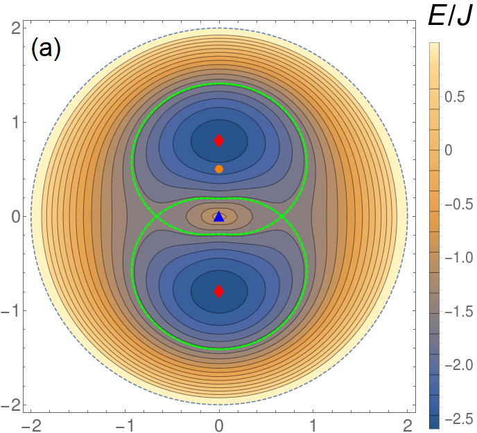
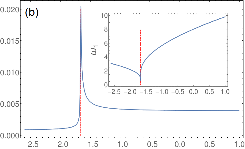
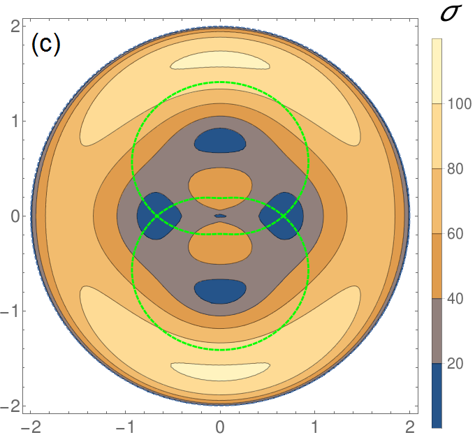
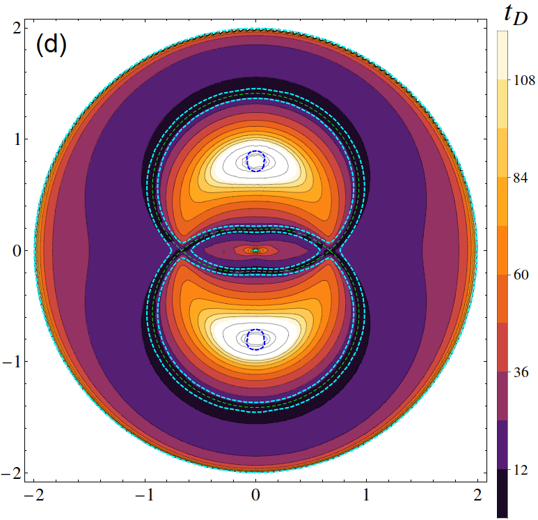
Using the semi-classical formulae for $\omega_{1}$ (19) and $e_{2}$ (21), and the analytical expression for the energy standard deviation $\sigma$ (35), we study their dependence and that of the decay time $t_{D}=\omega_{1}/(\sigma|e_{2}|)$ (24) on the parameters of the initial coherent states for the LMG model with couplings as in section III of the main text, $\gamma_{x}=-3,\gamma_{y}=-5$, and $J=2000$. A similar analysis can be performed for any other coupling set. The coherent parameter space defines the surface of the so-called Bloch sphere. For simplicity, this surface is represented in a 2D circle using coordinates $(1+j_{z})\cos\phi$ and $(1+j_{z})\sin\phi$. In this representation, the south pole is located in the center of the circle whereas the north pole is deformed to the outer circle of radius $2$. $\omega_{1}$ and $e_{2}$ are obtained by using the method described in Engelhardt2015 .

The results are shown in figure 9. In panel (a), level curves of the scaled energy are shown. Red diamonds indicate the ground-state configurations with $E/J=-2.6$. Dashed green line indicates the level curve of the ESQPT critical energy at $E_{ESQPT}/J=-1.6667$. The central blue triangle is a local maximum critical point at energy $E/J=-1$. The orange dot indicates the coordinate of the representative coherent-sate discussed in section III of the main text. The parameters $e_{2}$ and $\omega_{1}$ depend only on energy, their dependences are shown, respectively, in panel (b) and inset. The vertical dashed lines indicate the ESQPT critical energy, where $e_{2}$ diverges and $\omega_{1}=0$. Contrary to the latter parameters, the energy width $\sigma$ depends on the localization of the coherent states in the Bloch sphere, this dependence is shown in panel (c). The decay time of the $SP$ ($t_{D}$) as a function of the initial coherent state is shown in panel (d). In this panel, blue and cyan lines delimit the small regions around the critical energy configurations (ground-state and ESQPT respectively) where our approach is not applicable for $J=2000$ (we use the criterion $E\pm 3.5\sigma=E_{cr}$ to define these lines). These regions become narrower as $J$ approaches the classical ($J\rightarrow\infty$) limit. Observe that the decay time increases unboundedly for states approaching the ground state configuration or the local maximum in the center, whereas for states close to the ESQPT the decay time goes to zero. This latter result is in accord with those of Fernandez2011 .

A similar analysis of the $SP$ parameters for the Dicke model, is a challenging task, not only because the dimension of the energy surfaces is three, but also because the increase in the numbers of Gaussian sub-sequences makes it hard to provide a complete analysis. However, the different study cases used in the main text are representative of the whole cases that can be found in the regular regime of the Dicke model.

Appendix F Classical limit of the survival probability and power law decay of its revivals

In this section we derive analytically the classical limit of the survival probability, as well as the power law decay of its revivals.

The decay of the oscillations in the survival probability is given by the expression (26) with the first argument $x=0$. Taking the limit $J>>1$ and using $\omega_{1}\approx\omega_{cl}$, $\sigma\approx f_{\sigma}\sqrt{J}$, $e_{2}\approx f_{e}/J$ and $t_{D}=\omega_{1}/(\sigma|e_{2}|)$, the SP decay reads

$$SP^{Decay}(t)\!\approx\!\frac{\omega_{cl}}{2f_{\sigma}\sqrt{\pi}\sqrt{J}}\Theta_{3}\left(0,e^{-\frac{1}{J}\left[\frac{\omega_{cl}^{2}}{4f_{\sigma}^{2}}+\frac{f_{\sigma}^{2}f_{e}^{2}}{\omega_{cl}^{2}}t^{2}\right]}\right).$$

As $\lim_{J\rightarrow\infty}\Theta_{3}(0,e^{-b/J})/\sqrt{J}=\sqrt{\pi/b}$,

$$\lim_{J\rightarrow\infty}SP^{Decay}(t)=\frac{1}{\sqrt{1+\left(\frac{2f_{\sigma}^{2}f_{e}t}{\omega_{cl}^{2}}\right)^{2}}}\approx\frac{\omega_{cl}^{2}}{2\sigma^{2}|e_{2}|}\frac{1}{t}\leavevmode\nobreak\ \leavevmode\nobreak\ \leavevmode\nobreak\ (t>>1),$$ (43)

which explains the power-law decay observed in the survival probability at times $t\sim t_{D}$.

The partial revivals occurring at integer multiples of the classical period $\tau=2\pi/\omega_{cl}$ become more and more narrower as $J$ increases, turning into Kronecker deltas in the limit $J\rightarrow\infty$. The heights ($f_{n}$) of the widthless revivals are given by (43) evaluated in $t=n\tau=2\pi n/\omega_{cl}$, thus the $SP$ in the limit $J\rightarrow\infty$ is

$$\lim_{J\rightarrow\infty}SP(t)=\sum_{n\in\mathbb{Z}}\delta_{t,n\tau}f_{n},{\hbox{\ \ \ with \ \ \ }}f_{n}=\frac{1}{\sqrt{1+\left(\frac{4\pi f_{\sigma}^{2}f_{e}}{\omega_{cl}^{3}}\right)^{2}n^{2}}}.$$

Appendix G Interference terms

To derive an analytical expression for the interference terms $SP_{I}^{(ij)}$ given in (32) we write

$$SP_{I}^{(ij)}(t)\equiv\displaystyle\sum_{p\in\mathbb{Z}}SP_{Ip}^{(ij)}(t)=2\displaystyle\sum_{p\in\mathbb{Z}}\sum_{k}g_{k}^{(i)}g_{k+p}^{(j)}\cos\left[\Omega_{k}^{(p)}t\right],$$ (44)

with $\Omega_{k}^{(p)}=(E_{k+p}^{(i)}-E_{k}^{(i)}+\delta E_{ij})$, under the assumption $E_{k}^{(j)}=E_{k}^{(i)}+\delta E_{ij}.$

The product of the Gaussian functions $g_{k}^{(i)}g_{k+p}^{(j)}$ leads to another single Gaussian for the frequencies $\Omega_{k}^{(p)}$. To demonstrate this, we express $E_{k}^{(i)}$ as a function of $\Omega_{k}^{(p)}$ employing (11)

$$E_{k}^{(i)}=\frac{(\Omega_{k}^{(p)}-\delta E_{ij})^{2}}{4e_{2}p^{2}}-\frac{\Omega_{k}^{(p)}-\delta E_{ij}+2e_{o}}{2}-\frac{e_{1}^{2}-p^{2}e_{2}^{2}}{4e_{2}}.$$

Using this and (7), we obtain

$$g_{k}^{(i)}g_{k+p}^{(j)}=A_{i}A_{j}\exp\left[-\frac{(\bar{E}_{i}-\bar{E}_{j}+\Omega_{k}^{(p)})^{2}}{2(\sigma_{i}^{2}+\sigma_{j}^{2})}\right]\exp\left[-\frac{\sigma_{i}^{2}+\sigma_{j}^{2}}{2\sigma_{i}^{2}\sigma_{j}^{2}}G\left(\Omega_{k}^{(p)}\right)^{2}\right],$$

where $G$ is a quadratic function, $G=A_{p}\left(\Omega_{k}^{(p)}\right)^{2}+B_{p}\Omega_{k}^{(p)}+C_{p}$, with

$$A_{p}=\frac{1}{4e_{2}p^{2}},\ \ \ \ \ B_{p}=\frac{\sigma_{i}^{2}-\sigma_{j}^{2}}{2(\sigma_{i}^{2}+\sigma_{j}^{2})}-\frac{\delta E_{ij}}{2e_{2}p^{2}},$$

and

$$C_{p}=\frac{1}{4}\left(-\frac{e_{1}^{2}}{e_{2}}+4e_{o}+e_{2}p^{2}-\frac{4(\bar{E}_{j}\sigma_{i}^{2}+\bar{E}_{i}\sigma_{j}^{2})}{\sigma_{i}^{2}+\sigma_{j}^{2}}+2\delta E_{ij}+\frac{\delta E_{ij}^{2}}{e_{2}p^{2}}\right).$$

As in C, since the function $G^{2}$ is inside the argument of the exponential, we consider a Taylor expansion around its minimum ($\Omega_{p}^{ij}$) up to quadratic terms

$$G\left(\Omega_{k}^{(p)}\right)^{2}\approx(B_{p}^{2}-4A_{p}C_{p})(\Omega_{k}^{(p)}-\Omega_{p}^{ij})^{2}{\hbox{\ \ \ \ \ with \ \ \ \ }}\Omega_{p}^{ij}=\frac{-B_{p}\pm\sqrt{B_{p}^{2}-4A_{p}C_{p}}}{2A_{p}}.$$

At leading order in $e_{2}$

$$\Omega_{p}^{ij}\approx\delta E_{ij}+p\,\omega_{ij}{\hbox{\ \ \ \ \ and \ \ \ \ \ }}(B_{p}^{2}-4A_{p}C_{p})\approx\frac{\omega_{ij}^{2}}{4e_{2}^{2}p^{2}},$$

where $\omega_{ij}$ is given by

$$\omega_{ij}=\sqrt{e_{1}^{2}+4e_{2}\left[\frac{\bar{E}_{j}\sigma_{i}^{2}+\bar{E}_{i}^{2}\sigma_{j}^{2}-\delta E_{ij}\sigma_{i}^{2}}{\left(\sigma_{i}^{2}+\sigma_{j}^{2}\right)}-e_{0}\right]}.$$

The parameter $\omega_{ij}$ can be estimated from the numerical spectrum as described below.

With

$$\sigma_{ij}=\frac{2|e_{2}|\,\sigma_{i}\sigma_{j}}{\omega_{ij}\sqrt{\sigma_{i}^{2}+\sigma_{j}^{2}}},$$

the terms in the sum(44) now become

$$SP_{Ip}^{(ij)}(t)\approx 2A_{i}A_{j}e^{\left[-\frac{(\bar{E}_{i}-\bar{E}_{j}+\delta E_{ij}+p\omega_{ij})^{2}}{2(\sigma_{i}^{2}+\sigma_{j}^{2})}\right]}\sum_{k}\exp\left[-\frac{\left(\Omega_{k}^{(p)}-(\delta E_{ij}+p\omega_{ij})\right)^{2}}{2(p\sigma_{ij})^{2}}\right]\cos\left[\Omega_{k}^{(p)}t\right].$$

From (11), we obtain $\Delta\Omega^{(p)}=\Omega_{k+1}^{(p)}-\Omega_{k}^{(p)}=2pe_{2}$, to approximate the previous sum by an integral that can be calculated as in D,

$$SP_{Ip}^{(ij)}(t)\!\approx\!\frac{2A_{i}A_{j}\sqrt{2\pi}\sigma_{i}\sigma_{j}}{\omega_{ij}\sqrt{\sigma_{i}^{2}+\sigma_{j}^{2}}}e^{\left[-\frac{(p\sigma_{ij}t)^{2}}{2}\right]}\exp\!\!\left[-\frac{(\!\bar{E}_{i}-\!\bar{E}_{j}+\!\delta E_{ij}+\!p\omega_{ij})^{2}}{2(\sigma_{i}^{2}+\sigma_{j}^{2})}\right]\cos[(\delta E_{ij}+p\omega_{ij})t].$$

Finally, we present a simple way to estimate the parameter $\omega_{ij}$. According to the discussion above, the maximum of the product $g_{k}^{(i)}g_{k+1}^{(j)}$ is $\Omega_{p=1}^{(ij)}=\delta E_{ij}+\omega_{ij}$. On the other hand, the product of two Gaussian functions, considering the energy as a continuous variable $x$ and a fixed parameter $\Delta$, $g^{(i)}(x)g^{(j)}(x+\Delta)=A_{i}A_{j}\exp\left[-\frac{(x-\bar{E_{i}})^{2}}{2\sigma_{i}^{2}}\right]\exp\left[-\frac{(x+\Delta-\bar{E_{j}})^{2}}{2\sigma_{j}^{2}}\right],$ acquires its maximum value at $x_{max}=E_{ij}^{(I)}-\frac{\sigma_{i}^{2}}{\sigma_{i}^{2}+\sigma_{j}^{2}}\Delta,$ with

$$E_{ij}^{(I)}=\frac{\bar{E}_{i}\sigma_{j}^{2}+\bar{E}_{j}\sigma_{i}^{2}}{\sigma_{i}^{2}+\sigma_{j}^{2}}.$$ (45)

For the argument of the second Gaussian, we sum $x_{max}+\Delta=E_{ij}^{(I)}+\frac{\sigma_{j}^{2}}{\sigma_{i}^{2}+\sigma_{j}^{2}}\Delta$. Therefore the pair of continuous energies maximizing the product of Gaussians are located to the right and to the left of $E_{ij}^{(I)}$. Returning to the discrete spectrum, the best approximation to this pair of energies is given by the pair of consecutive discrete energies satisfying

$$E_{k_{I}}^{(i)}\leq E_{ij}^{(I)}\leq E_{k_{I}+1}^{(i)}.$$ (46)

From this simple observation, the frequency maximizing the Gaussian product can be approximated by $\Omega_{p=1}^{(ij)}\approx E_{k_{I}+1}^{(i)}+\delta E_{ij}-E_{k_{I}}^{(i)}$. Comparing this with the equivalent expression in terms of $\omega_{ij}$, that is $\Omega_{p=1}^{(ij)}=\delta E_{ij}+\omega_{ij}$, allows for the estimation

$$\omega_{ij}\approx E_{k_{I}+1}^{(i)}-E_{k_{I}}^{(i)}.$$

This provides a way to estimate $\omega_{ij}$ from the numerical spectrum by using (45) and (46).

References

- (1) Chu S 2002 Nature (London) 416 206
- (2) Bernien H, Schwartz S, Keesling A, Levine H, Omran A, Pichler H, Choi S, Zibrov A S, Endres M, Greiner M, Vuletić V and Lukin M D Probing many-body dynamics on a 51-atom quantum simulator arXiv:1707.04344
- (3) Blatt R and Roos C F 2012 Nat. Phys. 8 277–284
- (4) Richerme P, Gong Z X, Lee A, Senko C, Smith J, Foss-Feig M, Michalakis S, Gorshkov A V and Monroe C 2014 Nature (London) 511 198–201
- (5) Wei K X, Ramanathan C and Cappellaro P 2018 Phys. Rev. Lett. 120 070501 chains arXiv:1612.05249
- (6) Lipkin H J, Meshkov N and Glick A J 1965 Nucl. Phys. 62 188–198
- (7) Meshkov N, Glick A J and Lipkin H J 1965 Nucl. Phys. 62 199–210
- (8) Glick A J, Lipkin H J and Meshkov N 1965 Nucl. Phys. 62 211–224
- (9) Dicke R H 1954 Phys. Rev. 93 99
- (10) Hepp K and Lieb E H 1973 Ann. Phys. (N.Y.) 76 3600003-4916
- (11) Wang Y K and Hioe F T 1973 Phys. Rev. A 7(3) 831–836
- (12) G. J. Milburn, J. Corney, E. M. Wright, and D. F. Walls 1997 Phys. Rev. A 55 4318.
- (13) M. J. Steel and M. J. Collett 1998 Phys. Rev. A 57 2920.
- (14) Zibold T, Nicklas E, Gross C and Oberthaler M K 2010 Phys. Rev. Lett. 105(20) 204101
- (15) Baumann K, Guerlin C, Brennecke F and Esslinger T 2010 Nature (London) 464 1301
- (16) Baumann K, Mottl R, Brennecke F and Esslinger T 2011 Phys. Rev. Lett. 107 140402
- (17) Campbell S 2016 Phys. Rev. B 94 184403
- (18) Wang Q, Quan H T 2017 Phys. Rev. E 96 032142
- (19) Santos L F and Pérez-Bernal F 2015 Phys. Rev. A 92 050101
- (20) Santos L F, Távora M and Pérez-Bernal F 2016 Phys. Rev. A 94 012113
- (21) Pérez-Fernández P, Cejnar P, Arias J M, Dukelsky J, García-Ramos J E and Relaño A 2011 Phys. Rev. A 83(3) 033802
- (22) Heyl M, Polkovnikov A, and Kehrein S 2013 Phys. Rev. Lett. 110 135704
- (23) Heyl M 2018 Rep. Prog. Phys. 81 054001
- (24) Alhassid Y and Levine R D 1992 Phys. Rev. A 46 4650
- (25) E. J. Torres-Herrera and L. F. Santos, Phil. Trans. R. Soc. A 375, 20160434 (2017).
- (26) L. Fonda, G. C. Ghirardi, and A. Rimini, Rep. Prog. Phys., 41, 587 (1978).
- (27) R. Ketzmerick, G. Petschel, and T. Geisel, Phys. Rev. Lett. 69, 695 (1992).
- (28) L. A. Khalfin, Sov. Phys. JETP 6, 1053 (1958); J. G. Muga, A. Ruschhaupt, and A. del Campo, Time in Quantum Mechanics, vol. 2 (Springer, London 2009)
- (29) Peres A 1984 Phys. Rev. A 30 161
- (30) Gorin T, Prosen T, Seligman T H, Z̆nidaric̆ M 2006 Phys. Rep. 435 33
- (31) Prosen T and Z̆nidaric̆ M 2002 J. Phys. A: Math. Gen. 35 1455
- (32) Prosen T, Seligman T H, Z̆nidaric̆ M 2003 Phys. Rev. A 67 042112
- (33) Torres-Herrera E J and Santos L F 2014 Phys. Rev. A 89 043620,
- (34) Torres-Herrera E J, Vyas M and Santos L F 2014 New J. Phys. 16 063010,
- (35) Torres-Herrera E J and Santos L F 2014 Phys. Rev. E 89 062110
- (36) Torres-Herrera E J and Santos L F 2014 Phys. Rev. A 90 033623
- (37) Flambaum V V and Izrailev F M 2001 Phys. Rev. E 64 026124
- (38) Izrailev F M and Castañeda-Mendoza A 2006 Phys. Lett. A 350 355
- (39) Távora M, Torres-Herrera E J and Santos L F 2016 Phys. Rev. A 94 041603,
- (40) Távora M, Torres-Herrera E J and Santos L F 2017 Phys. Rev. A 95 013604
- (41) Torres-Herrera E J and Santos L F 2017 Ann. Phys. (Berl.) 529 1600284
- (42) Klauder J R and Skagerstam B-S 1985 Coherent States: Applications in Physics and Mathematical Physics (Singapore: World Scientific)
- (43) Zhang W-M, Feng D H, and Gilmore R 1990 Rev. Mod. Phys. 62 867
- (44) Altland A and Haake F 2012 New J. Phys. 14 073011
- (45) Altland A and Haake F 2012 Phys. Rev. Lett. 108 073601
- (46) Bakemeier L, Alvermann A and Fehske H 2013 Phys. Rev. A 88 043835
- (47) Leichtle C, Averbukh I S and Schleich W P 1996 Phys. Rev. A 54 5299–5312
- (48) Kloc M, Stránský P, Cejnar P 2018 Phys. Rev. A 98 013836
- (49) Vázquez-Sánchez H, Lerma-Hernández S, work in progress
- (50) Relaño A, Bastarrachea-Magnani M A and Lerma-Hernández S 2016 EPL 116 50005
- (51) Bastarrachea-Magnani M A, Relaño A, Lerma-Hernández S, López-del-Carpio B, Chávez-Carlos J and Hirsch J G 2016 J. Phys. A 50
- (52) Castaños O, López-Peña R, Hirsch J G and López-Moreno E 2005 Phys. Rev. B 72 012406
- (53) Emary C and Brandes T 2003 Phys. Rev. Lett. 90 044101
- (54) Emary C and Brandes T 2003 Phys. Rev. E 67 066203
- (55) Ribeiro A D, de Aguiar M A M and de Toledo Piza A F R 2006 J. Phys. A 39 3085
- (56) Larson J and Irish E K 2017 J. Phys. A 50 174002
- (57) Castaños O, Nahmad-Achar E, López-Peña R and Hirsch J G 2010 AIP Conf. Proc. 1323 40–51
- (58) Caprio M A, Cejnar P, Iachello F (2008) Ann. Phys. (N.Y.) 323 1106
- (59) Ribeiro P, Vidal J and Mosseri R 2008 Phys. Rev. E 78 021106
- (60) Bastarrachea-Magnani M A, Lerma-Hernández S and Hirsch J G 2014 Phys. Rev. A 89 032101
- (61) Stránský P, Macek M and Cejnar P 2014 Ann. Phys. (N.Y.) 345 73–97
- (62) Stránský P, Macek M, Leviatan A and Cejnar P 2015 Ann. Phys. (N.Y.) 356 57
- (63) Pérez-Bernal F and Santos L F 2017 Fortschr. Phys. 65 1600035
- (64) Engelhardt G, Bastidas V M, Kopylov W and Brandes T 2015 Phys. Rev. A 91 013631
- (65) Chen Q H, Zhang Y Y, Liu T and Wang K L 2008 Phys. Rev. A 78 051801
- (66) Liu T, Zhang Y Y, Chen Q H and Wang K L 2009 Phys. Rev. A 80 023810
- (67) Bastarrachea-Magnani M A and Hirsch J G 2014 Phys. Scr. 2014 014005
- (68) Hirsch J G and Bastarrachea-Magnani M A 2014 Phys. Scr. 2014 014018
- (69) Bastarrachea-Magnani M A, López-del-Carpio B, Chávez-Carlos J, Lerma-Hernández S and Hirsch J G 2016 Phys. Rev. E 93 022215
- (70) Torres-Herrera E J, Kollmar D and Santos L F 2015 Phys. Scr. T 165 014018
- (71) Schliemann J 2015 Phys. Rev. A 92 022108
- (72) Bastarrachea-Magnani M A, López-del-Carpio B, Chávez-Carlos J, Lerma-Hernández S and Hirsch J G 2017 Phys. Scr. 92 054003
- (73) Weisstein E W Jacobi theta functions MathWorld-A Wolfram Web Resource. http://mathworld.wolfram.com/JacobiThetaFunctions.html [September 2017]
- (74) Bastarrachea-Magnani M A, Lerma-Hernández S and Hirsch J G 2014 Phys. Rev. A 89 032102
- (75) Chávez-Carlos J, Bastarrachea-Magnani M A, Lerma-Hernández S and Hirsch J G 2016 Phys. Rev. E 94 022209
- (76) Lerma-Hernández S, Chávez-Carlos J, Bastarrachea-Magnani M A, López-del-Carpio B and Hirsch J G 2018, AIP Conf. Proc. 1950 030002
- (77) Reichl L E 2004 The transition to chaos: conservative classical systems and quantum manifestations (New York: Springer)
- (78) Wisniacki D A and Schlagheck P 2015 Phys. Rev. E 92 062923
- (79) Jaako T, Xiang Z-L, Garcia-Ripoll J J, and Rabl P 2016 Phys. Rev. A 94 033850
- (80) Felicetti S, Pedernales, J S, Egusquiza I L, Romero G, Lamata L, Braak D, and Solano E 2015 Phys. Rev. A 92 033817
- (81) Penna V, Raffa F A and Franzosi R 2018 J. Phys. A: Math. Theor. 51 045301