Spectral Algorithms for Computing Fair Support Vector Machines
Matt Olfat Anil Aswani
UC Berkeley UC Berkeley
Abstract
Classifiers and rating scores are prone to implicitly codifying biases, which may be present in the training data, against protected classes (i.e., age, gender, or race). So it is important to understand how to design classifiers and scores that prevent discrimination in predictions. This paper develops computationally tractable algorithms for designing accurate but fair support vector machines (SVM’s). Our approach imposes a constraint on the covariance matrices conditioned on each protected class, which leads to a nonconvex quadratic constraint in the SVM formulation. We develop iterative algorithms to compute fair linear and kernel SVM’s, which solve a sequence of relaxations constructed using a spectral decomposition of the nonconvex constraint. Its effectiveness in achieving high prediction accuracy while ensuring fairness is shown through numerical experiments on several data sets.
1 INTRODUCTION
The increasing prevalence of machine learning to automate decision-making systems has drawn societal scrutiny on the approaches used for verification and validation of these systems. In particular, two main concerns have been voiced with regards to the correctness and accuracy of decisions provided. The first is a general lack of interpretability for how predictions are produced by many learning techniques (Ridgeway et al., 1998; Lou et al., 2012; Caruana et al., 2015), and the second is the possibility of perpetuating inequities that may be present in the training data (Podesta et al., 2014; Barocas and Selbst, 2016; Bhandari, 2016).
This paper focuses on the latter: We study how to design fair support vector machines (SVM’s), and our goal is to construct a classifier that inputs predictors and a threshold , and predicts a label , while ensuring fairness with respect to a protected class (e.g., age, gender, or race). We assume there are only two protected classes; however, our formulations generalize to the setting with multiple protected classes.
We make four main contributions. First, we reinterpret two fairness notions using receiver operating characteristic (ROC) curves, which leads to a new visualization for classifier fairness. Second, we capture fairness by defining a constraint on covariance matrices conditioned on protected classes, which leads to a nonconvex quadratic constraint in the SVM formulation. Third, we construct an iterative algorithm that uses a spectral decomposition of the nonconvex constraint to compute fair linear and kernel SVM’s; we prove iterates converge to a local minimum. Fourth, we conduct numerical experiments to evaluate our algorithms.
1.1 Fairness Notions for Classifiers
Ensuring classifiers are fair requires quantifying their fairness. However, Friedler et al. (2016) and Kleinberg et al. (2016) showed that no single metric can capture all intuitive aspects of fairness, and so any metric must choose a specific aspect of fairness to quantify. In this paper, we consider the arguably two most popular notions: demographic parity (Calders et al., 2009; Zliobaite, 2015; Zafar et al., 2017) and equal opportunity (Dwork et al., 2012; Hardt et al., 2016). These notions are typically considered for a single threshold of the classifier, but here we will consider all possible thresholds. We believe this is more in-line with malicious usage of classifiers in which strategic choice of thresholds can be used to practice discrimination.
1.2 Algorithms to Compute Fair Classifiers
Several approaches have been developed to construct fair classifiers. Some (Zemel et al., 2013; Louizos et al., 2015) compute transformations of the data to make it independent of the protected class, though this can be too conservative and reduce predictive accuracy more than desired. Another method (Hardt et al., 2016) modifies any classifier to reduce its accuracy with respect to protected classes until fairness is achieved. Several techniques compute a fair classifier at a single threshold (Calders et al., 2009; Cotter et al., 2016); however, our interest is in classifiers that are fair at all thresholds. The only method we are aware of that tries to compute a fair classifier for all thresholds is that of Zafar et al. (2017), which will be our main comparison.
1.3 Outline
After describing the data and our notation in Section 2, we next define two fairness notions and provide a new ROC visualization of fairness in Section 3. Section 4 derives constraints to improve the fairness of linear and kernel SVM’s at all thresholds. This involves nonconvex constraints, and in Section 5 we present iterative algorithms that compute fair linear and kernel SVM’s by solving a sequence of convex problems defined using a spectral decomposition. Section 6 conducts numerical experiments using both synthetic and real datasets to demonstrate the efficacy of our approach in computing accurate but fair SVM’s.
2 DATA AND NOTATION
Our data consists of 3-tuples for points, where are predictors, are labels, and label a protected class. For a matrix , the -th row of is denoted . Define , , and to be matrices such that , , and , respectively.
Let be the set of indices for protected class is negative, and similarly let be the set of indices for which the protected class is positive. We use and for the cardinality of the sets and , respectively. Now define to be a matrix whose rows are for , and similarly define to be a matrix whose rows are for . Let and be the covariance matrices of and , respectively.
Next let be a kernel function, and consider the notation
| (1) |
Recall that the essence of the kernel trick is to replace with , and so the benefit of the matrix notation given in (1) is that it allows us to replace with as part of the kernel trick.
Last, we define some additional notation. Let , and note is the indicator function. A positive semidefinite matrix is denoted . If are vectors of equal dimension, then the notation refers to their element-wise product: . Also, is the vector whose entries are all 1.
3 ROC Visualization of Fairness
3.1 Demographic Parity
One popular notion of fairness is that predictions of the label are independent of the protected class . This definition is typically stated (Calders et al., 2009; Zliobaite, 2015; Zafar et al., 2017) in terms of a single threshold, though it can be generalized to multiple thresholds. We say that a classifier has demographic parity at level (abbreviated as DP-) if
| (2) |
To understand this, note is the true positive rate when predicting the protected class at threshold , while is the false positive rate when predicting the protected class at threshold . So the intuition is that a classifier is DP- if its false positive rates and true positive rates are approximately (up to deviation) equal at all threshold levels for the protected class.
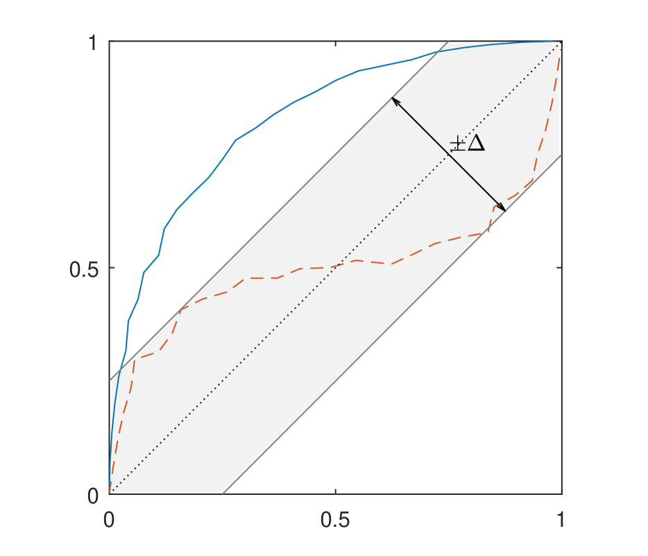
Reinterpreted, demographic parity requires that predictions of the classifier cannot reveal information about the protected class any better (up to deviation) than random guessing. DP- is in fact equivalent to requiring that the ROC curve for the classifier in predicting is within of the line of no-discrimination, which is the line that is achievable by biased random guessing. More visually, Figure 1 shows how DP- can be seen using an ROC curve.
3.2 Equal Opportunity
Demographic parity has been criticized as too strict (Dwork et al., 2012; Hardt et al., 2016), and so another notion of fairness has been proposed in which predictions of the label are independent of the protected class , when the true label is positive (i.e., ). In this definition, we must interpret as a better label than ; for instance, may be a loan default, while is full repayment of a loan. This definition is typically stated (Hardt et al., 2016) in terms of a single threshold, though it can be generalized to multiple thresholds. We say that a classifier has equal opportunity with level (abbreviated as EO-) if
| (3) |
To understand this, note is the true positive rate conditioned on when predicting the protected class at threshold , while is the false positive rate conditioned on when predicting the protected class at threshold . So the intuition is that a classifier is EO- if its false positive rates and true positive rates are approximately (up to deviation) equal at all threshold levels for the protected class, when conditioned on .
Reinterpreted, equal opportunity requires that predictions of the classifier cannot reveal information about the protected class any better (up to deviation) than random guessing, when the true label is positive. EO- is equivalent to requiring that the ROC curve for the classifier in predicting conditioned on is within of the line of no-discrimination. Figure 1 shows how DP- can be seen using an ROC curve.
4 FAIRNESS CONSTRAINTS
In this section, we derive several fairness constraints for linear SVM. The kernel trick is used to convert these constraints for use in kernel SVM. We will focus on presenting formulations for demographic parity, though all of our formulations easily generalize to equal opportunity by simply conditioning on .
4.1 Constraints for Linear SVM
We first study constraints that can be used to ensure fairness with respect to for a linear SVM
| (4) |
where , are coefficients to predict the label . Consider the following generic linear SVM formulation
| (5) | ||||||
| s.t. | ||||||
where is a tuning parameter that can be chosen using cross-validation, and is a fairness constraint with the fairness level controlled by the (possibly vector-valued) parameter . We will next consider several possibilities for .
4.1.1 Indicator Constraints
The definition of DP- in (2) uses probabilities, which are are not available as data. Fortunately, we can use empirical fractions of events as an approximation:
| (6) |
The above is difficult to include in the linear SVM as the fairness constraint , because it involves the discontinuous and nonconvex function, and is infinite-dimensional since it must hold for all .
4.1.2 Integer Constraints
An initial idea to incorporate (6) in the linear SVM is based on recent empirical results (Miyashiro and Takano, 2015; Bertsimas et al., 2016) where mixed integer programming (MIP) was used to exactly solve cardinality constrained linear regression. Specifically, we can approximate the indicator constraints (6) as the following mixed-integer linear inequalities
| (7) | ||||
for ; where is a large constant, and is a fixed set of values. This removes the function, and it ensures a finite number of constraints. However, we found in numerical experiments using Gurobi (2016) and Mosek (2017) that computing a fair linear SVM with the above constraints was prohibitively slow except for very small data sets.
4.1.3 Convex Relaxation
We next derive a convex relaxation of the indicator constraints (6). Let be a constant, and consider . Then convex upper bounds for the indicators are and . Using these upper bounds on (6) leads to the following convex relaxation
| (8) |
where . There are three important remarks about this convex relaxation. The first is that the threshold does not appear, which means this is simply a linear constraint. The second is that the bound can be subsumed into the parameter used to control the fairness level, meaning that this relaxation is practically independent of the bound . The third is that this convex relaxation is equivalent to the fairness constraint proposed by Zafar et al. (2017), though they derive this using a correlation argument.
4.1.4 Covariance Constraints
The convex relaxation (8) is fairly weak, and so it is relevant to ask whether constraints can be added to (8) to increase the fairness level of the resulting linear SVM. Instead of using convex lifts (Lasserre, 2001; Gouveia et al., 2013; Chandrasekaran and Jordan, 2013) to tighten the above constraint, we take a geometric approach to derive new constraints.
Specifically, consider the two conditional distributions and . Observe that the conditional distributions of and have mean and , respectively. This means (8) can be interpreted as requiring
| (9) |
or equivalently that the means of when conditioned on are approximately (i.e., up to apart) equal. Thus it is natural to consider adding constraints to match the conditional distributions of using higher order moments.
Here, we define a constraint to ensure that the covariances of conditioned on are approximately equal. Let and be the sample covariance matrices for and , respectively. Then the sample variances of and are and , respectively. So we specify our covariance constraint as
| (10) |
To our knowledge, this constraint has not been previously used to improve the fairness of classifiers. Unfortunately, it is nonconvex because is symmetric but typically indefinite (i.e., not positive or negative semidefinite). Hence, computing a linear SVM with this constraint requires further development.
One obvious approach is to lift the constraint (10) and then construct a semidefinite programming (SDP) relaxation (Goemans and Williamson, 1995; Luo et al., 2010). Specifically, note that (10) is equivalent to
| (11) | ||||
The above is nonconvex, but it can be convexified by dropping the constraint. However, we found in numerical experiments using the Mosek (2017) solver that the SDP relaxation was weak and did not consistently affect the fairness or accuracy of the SVM. Despite this result, we believe that additional convexification techniques (Kocuk et al., 2016; Madani et al., 2017) can be used to strengthen the quality of the SDP relaxation; we leave the problem of how to design a strengthened SDP relaxation for future work.
4.2 Constraints for Kernel SVM
We next study constraints that can be used to ensure fairness with respect to for a kernel SVM
| (12) |
where are coefficients to predict the label , and with the set of indices . Consider the following generic kernel SVM formulation
| (13) | ||||
| s.t. | ||||
where is a tuning parameter that can be chosen using cross-validation, and is a fairness constraint with the fairness level controlled by the (possibly vector-valued) parameter . We will next consider several possibilities for .
4.2.1 Indicator and Integer Constraints
The indicator constraints (6) can be rewritten for kernel SVM by replacing (4) with (12). Unfortunately, the indicator constraints are still impractical because they are infinite-dimensional and contain a discontinuous, nonconvex function. However, we can approximate the indicator constraints for kernel SVM as the following mixed-integer linear inequalities
| (14) | ||||
for ; where is a large constant, and is a fixed set of values. However, we found in numerical experiments using the Gurobi (2016) and Mosek (2017) solvers that computing a fair kernel SVM with the above constraints was prohibitively slow except for very small data sets.
4.2.2 Convex Relaxation
We next provide a convex relaxation of the indicator constraints for kernel SVM. A similar argument as the one used for linear SVM gives
| (15) |
Note that threshold does not appear, which means this is simply a linear constraint on .
4.2.3 Covariance Constraints
Our covariance constraint can be rewritten for the kernel SVM by first recalling that the kernel SVM with generates the same classifier as directly solving a linear SVM. Thus, we have the relationship in this special case. Next, observe that
| (16) | ||||
So if apply the kernel trick to our covariance constraint (10) with the above relationships, then the resulting covariance constraint for kernel SVM becomes
| (17) |
where we have
| (18) | ||||
The constraint (17) is a nonconvex quadratic constraint because is symmetric but typically indefinite (i.e., not positive or negative semidefinite).
We can also construct an SDP relaxation of (17). Specifically, note that (17) is equivalent to
| (19) | ||||
The above is nonconvex, but it can be convexified by dropping the constraint. However, our numerical experiments using the Mosek (2017) solver found the SDP relaxation was weak and did not consistently affect the fairness or accuracy of the SVM.
5 SPECTRAL ALGORITHM
The covariance constraints are conceptually promising, but they result in nonconvex optimization problems. Here, we describe an iterative algorithm to effectively solve the SVM with our covariance constraints.
5.1 Linear SVM
Though we could compute the linear SVM with the covariance constraint (10) using successive linearization, a better approach is possible through careful design of the algorithm: Our key observation regarding (10) is that is symmetric, which means it can be diagonalized by an orthogonal matrix:
| (20) |
where and the form an orthonormal basis. Now let and , and define the positive semidefinite matrices
| (21) | ||||
This means that the function
| (22) |
in the covariance constraint (10) is the difference of the two convex functions and .
There is an important point to note regarding the practical importance of the spectral decomposition we performed above. The function in the covariance constraint (10) can alternatively be written as the difference of the two convex functions and . However, using this alternative decomposition yields an algorithm where the convexified subproblems are weaker relaxations than the convex subproblems generated using the spectral decomposition. As a result, our algorithm given below is ultimately more effective because it employs the spectral decomposition.
Consequently, the constrained convex-concave procedure (Tuy, 1995; Yuille and Rangarajan, 2002; Smola et al., 2005) can be used to design an algorithm for our setting. We opt to use a penalized form of the quadratic constraint in our spectral algorithm to ensure feasibility always holds. Let be a fixed point, and consider the optimization problem where the concave terms are linearized:
| (23) | ||||
| s.t. | ||||
Our spectral algorithm for computing a fair linear SVM consists of the constrained CCP adapted to the problem of computing a linear SVM with the linear constraint (8) and covariance constraint (10): We initialize by solving a linear SVM with only the linear constraint (8), and then computing successive by solving (23). This produces a local minimum.
Theorem 1 (Smola et al. (2005))
The spectral algorithm defined above for computing a fair linear SVM gives iterates that converge to a local minimum.
This theorem is simply an application of a theorem by Smola et al. (2005), and the constraint qualification required by this theorem trivially holds in our case because all of our convex constraints are linear.
5.2 Kernel SVM
We can also design a spectral algorithm to compute fair kernel SVM’s. Since in (17) is symmetric, t can be diagonalized by an orthogonal matrix:
| (24) |
where and the form an orthonormal basis. Now let and , and define the positive semidefinite matrices
| (25) | ||||
This means that the function
| (26) |
in (17) is the difference of the two convex functions and .
Thus, the constrained convex-concave procedure (Tuy, 1995; Yuille and Rangarajan, 2002; Smola et al., 2005) can be used to design an algorithm. We use a penalized form of the quadratic constraint in our spectral algorithm to ensure feasibility always holds. Let be a fixed point, and consider the optimization problem where the concave terms are linearized:
| (27) | ||||
| s.t. | ||||
Our spectral algorithm for computing a fair kernel SVM consists of the constrained CCP adapted to the problem of computing a kernel SVM with the linear constraint (15) and covariance constraint (17): We initialize by solving a kernel SVM with only the linear constraint (15), and then computing successive by solving (23). This produces a local minimum.
Theorem 2 (Smola et al. (2005))
The spectral algorithm defined above for computing a fair kernel SVM gives iterates that converge to a local minimum.
This theorem is simply an application of a theorem by Smola et al. (2005), and the constraint qualification required by this theorem trivially holds in our case because all of our convex constraints are linear.
6 NUMERICAL EXPERIMENTS
We use synthetic and real datasets to evaluate the efficacy of our approach. We compare linear SVM’s computed using our spectral algorithm (SSVM) to a standard linear SVM (LSVM) and a linear SVM computed using the approach of Zafar et al. (2017) (ZSVM), since this is the only existing approach that to our knowledge is designed to ensure fairness at all thresholds.
6.1 Synthetic Data

Experimental Design
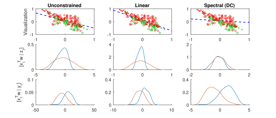
We seek to examine the case in which our and labels are correlated, and and have differing covariances. Thus, we generate 200 data points where the and labels are generated through logit models using two separate sets of randomly generated “true” parameters, with dot product between the logit parameters of and of 0.85. The singular values of the covariance matrix of were then skewed to generate the data seen in Figure 2. The empirical correlation of and is 0.45.
Results
The results of the three methods using and are shown in the three columns of Figure 2. Here, points in and are differentiated by marker shape (“x” and “o”, respectively), and points with label and are differentiated by color (red and green, respectively). If denotes the coefficients computed by each method, then the second row shows the empirical densities of conditioned on the protected class , and the third row shows the empirical densities of conditioned on the label . Fairness occurs if the conditional densities in the second row are similar, and prediction accuracy occurs if the densities in the third row are disparate. These results show that the densities of and are distinguishable for SSVM and ZSVM, while they are almost identical for SSVM. On the other hand, the densities of and are distinct for all three methods.
6.2 Real World Datasets
Data overview
We next use a wine quality dataset Cortez et al. (2009) and a dataset of German credit card customers (Lichman, 2013). The first dataset is a compilation of 12 attributes of 6,497 wines (e.g., acidity, residual sugar, alcohol content, and color), as well as a ranking out of 10 that is provided by professional taste-testers. Here, we label when a wine is rated as a 6 or above and otherwise, and we define for white wines and for reds. Notably, all explanatory variables are continuous. The second dataset is a compilation of 20 attributes (e.g., marriage, employment and housing status, number of existing credit lines, and age) of 1000 German applicants for loans. We label for applicants that defaulted and for applicants that did not default, and let for applicants that are renting a home and for applicants that own their home. Note that a large number of variables are discrete. There is no missing data in either dataset.
Metrics of comparison
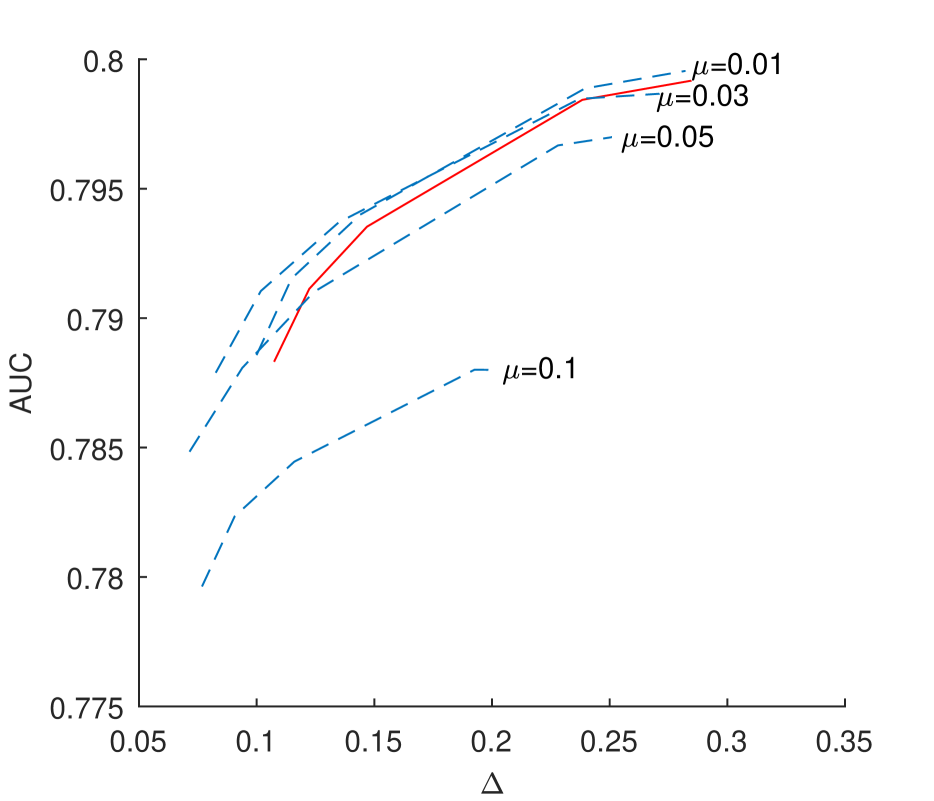
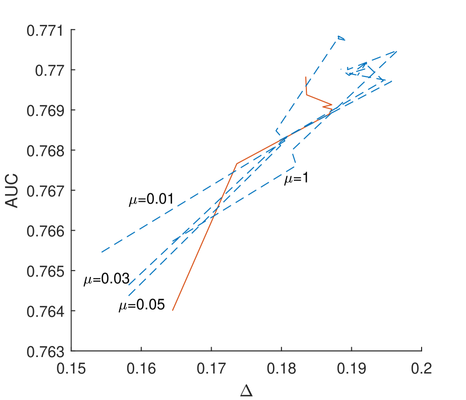
We compare SSVM and ZSVM based on the tradeoffs that they make between predictive accuracy for , measured using the area under the ROC curve (AUC), and their fairness with respect , measured by DP- with respect to .
Experimental Design
We conducted five rounds of cross-validation on each dataset and computed the average AUC and average , using a 70-30 training-testing split. Within each round, we first apply -fold cross-validation on LSVM to choose the that maximizes AUC, and this value of was used with both SSVM and ZSVM to minimize the impact of cross-validation on the comparison between methods. We varied over the values 0, 0.001, 0.002, 0.005, 0.01, 0.025, 0.05 and 0.1. And for SSVM we tried several values of , which are shown in our plots.
Results
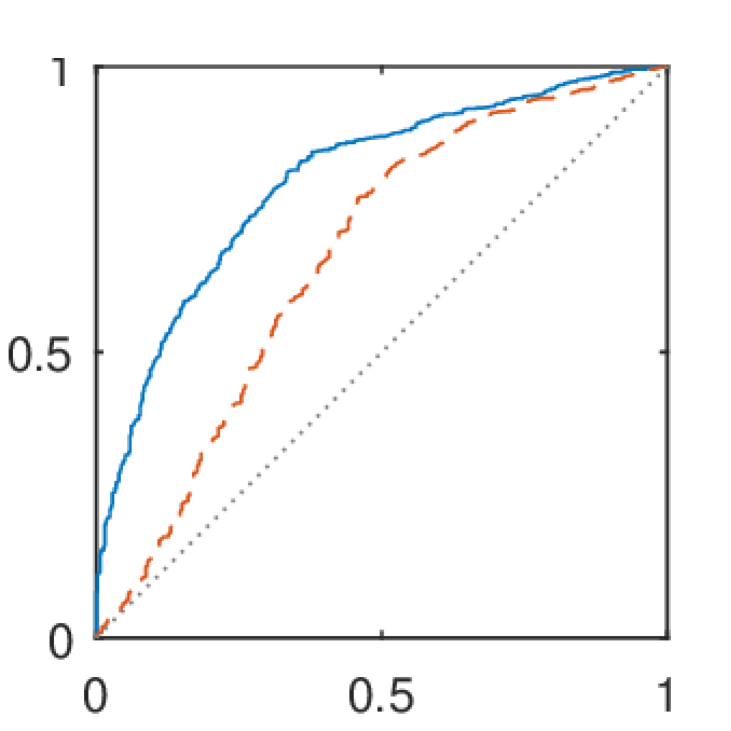
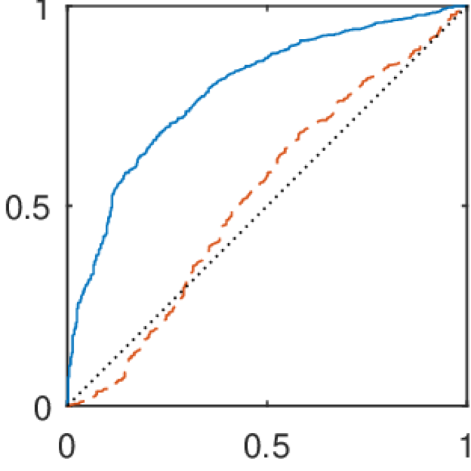
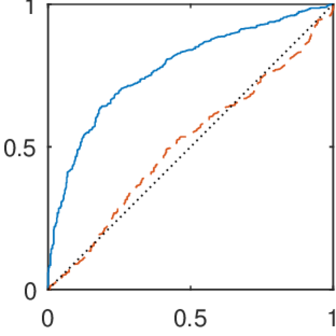
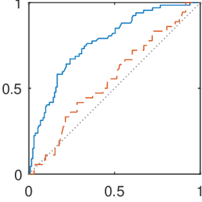
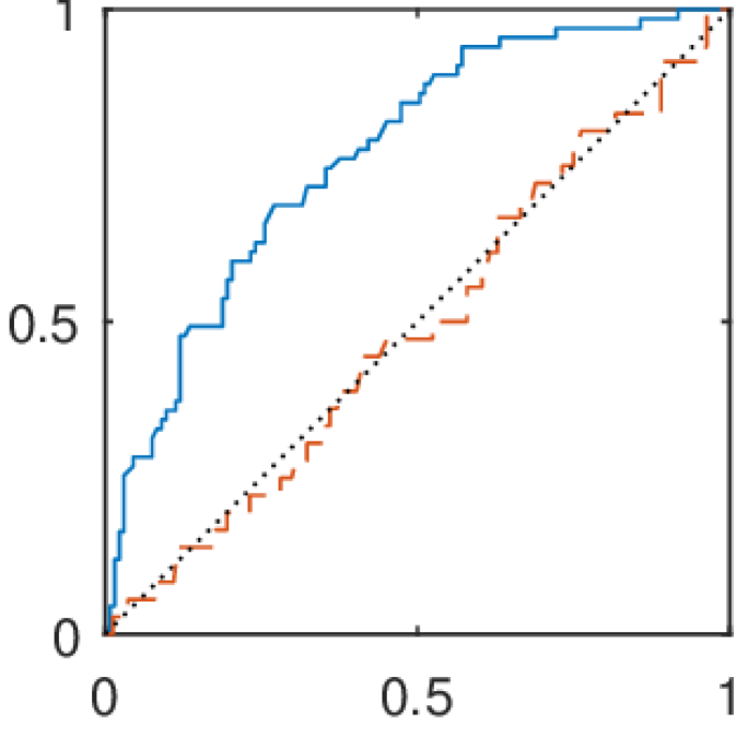
Figure 3 shows representative examples of ROC curves for both datasets from one instance of cross-validation. Both ZSVM and SSVM improve fairness with respect to LSVM while maintaining high accuracy, and SSVM ensures an even stricter level of fairness than LSVM while keeping high accuracy. The tradeoff curves between prediction accuracy and fairness are shown in Figure 4. Increasing generally jointly decreases fairness and increases accuracy, while small increases in for our SSVM can often improve both fairness and accuracy. Large increases in generally increase fairness but decrease accuracy. Note that setting leads to the curve for SSVM to align with the curve of ZSVM, since they are equivalent when . Also observe that is more sensitive to changes in and than the AUC, which implies that we are able control fairness without losing much predictive accuracy.
7 Conclusion
We considered multi-threshold notions of fairness for classifiers, and designed a nonconvex constraint to improve the fairness of linear and kernel SVM’s under all thresholds. We developed an iterative optimization algorithm (that uses a spectral decomposition) to handle our nonconvex constraint in the resulting problem to compute the SVM, and empirically compared our approach to standard linear SVM and an SVM with a linear fairness constraint using both synthetic and real data. We found that our method can strictly improve the fairness of classifiers for all thresholding values with little loss in accuracy; in fact, some of our results even showed a slight increase in accuracy with increasing fairness. Our work opens the door for further research in a number of areas, including hierarchies of fairness constraints considering subsequent moments of the data, and theoretical guarantees on the fairness of such classification methods.
References
- Barocas and Selbst [2016] S. Barocas and A. D. Selbst. Big data’s disparate impact. California Law Review, 104, 2016.
- Bertsimas et al. [2016] D. Bertsimas, A. King, and R. Mazumder. Best subset selection via a modern optimization lens. Annals of Statistics, 44(2):813–852, 2016.
- Bhandari [2016] E. Bhandari. Big data can be used to violate civil rights laws, and the FTC agrees, 2016.
- Calders et al. [2009] T. Calders, F. Kamiran, and M. Pechenizkiy. Building classifiers with independency constraints. In Data mining workshops, 2009. ICDMW’09. IEEE international conference on, pages 13–18. IEEE, 2009.
- Caruana et al. [2015] R. Caruana, Y. Lou, J. Gehrke, P. Koch, M. Sturm, and N. Elhadad. Intelligible models for healthcare: Predicting pneumonia risk and hospital 30-day readmission. In Proceedings of the 21st ACM SIGKDD International Conference on Knowledge Discovery and Data Mining, pages 1721–1730. ACM, 2015.
- Chandrasekaran and Jordan [2013] V. Chandrasekaran and M. I. Jordan. Computational and statistical tradeoffs via convex relaxation. Proceedings of the National Academy of Sciences, 110(13):E1181–E1190, 2013.
- Cortez et al. [2009] P. Cortez, A. Cerdeira, F. Almeida, T. Matos, and J. Reis. Modeling wine preferences by data mining from physicochemical properties. Decision Support Systems, 47(4):547–553, 2009.
- Cotter et al. [2016] A. Cotter, M. Friedlander, G. Goh, and M. Gupta. Satisfying real-world goals with dataset constraints. arXiv preprint arXiv:1606.07558, 2016.
- Dwork et al. [2012] C. Dwork, M. Hardt, T. Pitassi, O. Reingold, and R. Zemel. Fairness through awareness. In Proceedings of the 3rd Innovations in Theoretical Computer Science Conference, pages 214–226. ACM, 2012.
- Friedler et al. [2016] S. A. Friedler, C. Scheidegger, and S. Venkatasubramanian. On the (im) possibility of fairness. arXiv preprint arXiv:1609.07236, 2016.
- Goemans and Williamson [1995] M. X. Goemans and D. P. Williamson. Improved approximation algorithms for maximum cut and satisfiability problems using semidefinite programming. Journal of the ACM (JACM), 42(6):1115–1145, 1995.
- Gouveia et al. [2013] J. Gouveia, P. A. Parrilo, and R. R. Thomas. Lifts of convex sets and cone factorizations. Mathematics of Operations Research, 38(2):248–264, 2013.
- Gurobi [2016] Gurobi. Gurobi optimizer reference manual, 2016. URL http://www.gurobi.com.
- Hardt et al. [2016] M. Hardt, E. Price, and N. Srebro. Equality of opportunity in supervised learning. In Advances in Neural Information Processing Systems, pages 3315–3323, 2016.
- Kleinberg et al. [2016] J. Kleinberg, S. Mullainathan, and M. Raghavan. Inherent trade-offs in the fair determination of risk scores. arXiv preprint arXiv:1609.05807, 2016.
- Kocuk et al. [2016] B. Kocuk, S. S. Dey, and X. A. Sun. Inexactness of sdp relaxation and valid inequalities for optimal power flow. IEEE Transactions on Power Systems, 31(1):642–651, 2016.
- Lasserre [2001] J. B. Lasserre. Global optimization with polynomials and the problem of moments. SIAM Journal on Optimization, 11(3):796–817, 2001.
- Lichman [2013] M. Lichman. UCI machine learning repository, 2013. URL http://archive.ics.uci.edu/ml.
- Lou et al. [2012] Y. Lou, R. Caruana, and J. Gehrke. Intelligible models for classification and regression. In Proceedings of the 18th ACM SIGKDD international conference on Knowledge discovery and data mining, pages 150–158. ACM, 2012.
- Louizos et al. [2015] C. Louizos, K. Swersky, Y. Li, M. Welling, and R. Zemel. The variational fair autoencoder. arXiv preprint arXiv:1511.00830, 2015.
- Luo et al. [2010] Z.-Q. Luo, W.-K. Ma, A. M.-C. So, Y. Ye, and S. Zhang. Semidefinite relaxation of quadratic optimization problems. IEEE Signal Processing Magazine, 27(3):20–34, 2010.
- Madani et al. [2017] R. Madani, S. Sojoudi, G. Fazelnia, and J. Lavaei. Finding low-rank solutions of sparse linear matrix inequalities using convex optimization. SIAM Journal on Optimization, 27(2):725–758, 2017.
- Miyashiro and Takano [2015] R. Miyashiro and Y. Takano. Mixed integer second-order cone programming formulations for variable selection in linear regression. European Journal of Operational Research, 247(3):721–731, 2015.
- Mosek [2017] Mosek. The MOSEK optimization toolbox for MATLAB manual, 2017.
- Podesta et al. [2014] J. Podesta, P. Pritzker, E. Moniz, J. Holdren, and J. Zients. Big data: Seizing opportunities, preserving values. Executive Office of the President, 2014.
- Ridgeway et al. [1998] G. Ridgeway, D. Madigan, T. Richardson, and J. O’Kane. Interpretable boosted naïve bayes classification. In KDD, pages 101–104, 1998.
- Smola et al. [2005] A. J. Smola, S. Vishwanathan, and T. Hofmann. Kernel methods for missing variables. In AISTATS, 2005.
- Tuy [1995] H. Tuy. Dc optimization: theory, methods and algorithms. In Handbook of global optimization, pages 149–216. Springer, 1995.
- Yuille and Rangarajan [2002] A. L. Yuille and A. Rangarajan. The concave-convex procedure (cccp). In Advances in neural information processing systems, pages 1033–1040, 2002.
- Zafar et al. [2017] M. B. Zafar, I. Valera, M. G. Rodriguez, and K. P. Gummadi. Fairness constraints: Mechanisms for fair classification. In Proceedings of the 20th International Conference on Artificial Intelligence and Statistics, 2017.
- Zemel et al. [2013] R. Zemel, Y. Wu, K. Swersky, T. Pitassi, and C. Dwork. Learning fair representations. In Proceedings of the 30th International Conference on Machine Learning (ICML-13), pages 325–333, 2013.
- Zliobaite [2015] I. Zliobaite. On the relation between accuracy and fairness in binary classification. arXiv preprint arXiv:1505.05723, 2015.