Non-covalent interactions across organic and biological subsets of chemical space: Physics-based potentials parametrized from machine learning

Abstract

Classical intermolecular potentials typically require an extensive parametrization procedure for any new compound considered. To do away with prior parametrization, we propose a combination of physics-based potentials with machine learning (ML), coined IPML, which is transferable across small neutral organic and biologically-relevant molecules. ML models provide on-the-fly predictions for environment-dependent local atomic properties: electrostatic multipole coefficients (significant error reduction compared to previously reported), the population and decay rate of valence atomic densities, and polarizabilities across conformations and chemical compositions of H, C, N, and O atoms. These parameters enable accurate calculations of intermolecular contributions—electrostatics, charge penetration, repulsion, induction/polarization, and many-body dispersion. Unlike other potentials, this model is transferable in its ability to handle new molecules and conformations without explicit prior parametrization: All local atomic properties are predicted from ML, leaving only eight global parameters—optimized once and for all across compounds. We validate IPML on various gas-phase dimers at and away from equilibrium separation, where we obtain mean absolute errors between 0.4 and 0.7 kcal/mol for several chemically and conformationally diverse datasets representative of non-covalent interactions in biologically-relevant molecules. We further focus on hydrogen-bonded complexes—essential but challenging due to their directional nature—where datasets of DNA base pairs and amino acids yield an extremely encouraging 1.4 kcal/mol error. Finally, and as a first look, we consider IPML for denser systems: water clusters, supramolecular host-guest complexes, and the benzene crystal.

I Introduction

Our understanding of the physical laws that govern molecular interactions have led to an ever-improving description of the high-dimensional potential energy surface of condensed molecular systems. A variety of computational methods provide various approximations thereof: while high-level methods (e.g., coupled cluster) are restricted to a small number of atoms, other electronic-structure methods (e.g., density functional theory—DFT) can reach larger system sizes of up to $10^{2}-10^{3}$ atoms. Beyond this limit, classical potentials and force fields provide a much faster estimate of the interactions, enabling the calculation of thermodynamic and even kinetic properties for complex materials.

Many classical potentials and force fields are often termed physics-based because they encode assumptions about the governing physics of the interactions via their functional forms. Despite their widespread interest by the community, classical potentials are currently limited to a narrow set of molecules and materials, due to tedious and non-systematic parametrization strategies. Additive (i.e., non-polarizable) atomistic force fields are typically parametrized from a combination of ab initio calculations and experimental measurements, e.g., pure-liquid density, heat of vaporization, or NMR chemical shifts. Ensuring the accurate reproduction of various molecular properties, from conformational changes to thermodynamic properties (e.g., free energy of hydration), but also consistency across all other molecules parametrized remains challenging, time consuming, and difficult to automate.

Recently, a number of studies have brought forward the idea of more automated parametrizations. For instance, QMDFF is based on reference DFT calculations to parametrize a set of classical potentials.Grimme (2014) We also point out the automatic generation of intermolecular energiesMetz, Piszczatowski, and Szalewicz (2016) extracted from reference symmetry-adapted perturbation theoryJeziorski, Moszynski, and Szalewicz (1994) (SAPT) calculations. Interestingly, recent efforts have aimed at parametrizing potentials and force fields from atom-in-molecule (AIM) properties. Van Vleet et al.Van Vleet et al. (2016) and Vandenbrande et al.Vandenbrande et al. (2017) showed that a systematic use of AIMs can significantly reduce the number of global parameters to scale the individual energetic contributions. Overall, they propose AIMs as a means to more systematically parametrize models. Similar conclusions were reached for the additive OPLS force field,Cole et al. (2016) for which the missing polarization effects make a systematic scheme all the more challenging. These methodologies still require a number of a priori reference electronic-structure calculations to optimize various parameters of any new molecule encountered.

In the context of developing classical potentials for in silico screening across large numbers of compounds, the necessary computational investment for the parametrization procedures of each new molecule can become daunting. A radically different strategy consists in predicting the potential energy surface of a system from machine learning (ML).Bartók et al. (2010); Li, Kermode, and De Vita (2015); Behler (2016) ML encompasses a number of statistical models that improve their accuracy with data. Recent studies have reported unprecedented accuracies in reproducing reference energies from electronic-structure calculations, effectively offering a novel framework for accurate intramolecular interactions freed from molecular-mechanics-type approximations (e.g., harmonic potential).Chmiela et al. (2017); Botu et al. (2016); Schütt et al. (2017) While they do away with free parameters that need optimization (i.e., unlike force fields), they typically suffer from limited transferability: an ML model is inherently limited to interpolating across the training samples. A model trained on water clusters can be remarkably accurate toward describing liquid-state properties (e.g., pair-correlation functions), but remains specific to interactions solely involving water.Natarajan, Morawietz, and Behler (2015) Transferability of an ML model that would predict interactions across chemical compound space (i.e., the diversity of chemical compounds) stands nowadays as computationally intractable. Part of the reason is the necessity to interpolate across all physical phenomena for any geometry, as these models are driven by experience, rather than physical principles. Symmetries and conservation laws will require large amounts of data to be appropriately satisfied, if they are not correctly encoded a priori.

In this work, we propose a balance between the aforementioned physics-based models and an ML approach, coined IPML. To best take advantage of both approaches, we choose to rely on a physics-based model, where most parameters are predicted from ML. This approach holds two main advantages: ($i$) Leverage our understanding of the physical interactions at hand, together with the associated symmetries and functional forms, and ($ii$) Alleviate the reference calculations necessary to optimize the parameters of each new molecule.

The aforementioned AIM-based classical potentials, in this respect, offer an interesting strategy: they largely rely on perturbation theory to treat the long-range interactions (i.e., electrostatics, polarization, and dispersion), while overlap models of spherically-symmetric atomic densities describe the short-range interactions. Both theoretical frameworks estimate interaction energies from monomer properties—thereby significantly reducing the ML challenge from learning interactions between any combination of molecules to the much simpler prediction of (isolated) atomic properties. Incidentally, learning atomic and molecular properties have recently been the subject of extended research, providing insight into the appropriate representations and ML models.Rupp et al. (2012); Hansen et al. (2013); Ramakrishnan and von Lilienfeld (2017); Schütt et al. (2017) Parametrizing small-molecule force fields based on ML has already shown advantageous at a more coarse-grained resolution.Bereau and Kremer (2015) At the atomistic level, Bereau et al. had shown early developments of learning AIM properties, namely distributed multipole coefficients to describe the electrostatic potential of a molecule.Bereau, Andrienko, and von Lilienfeld (2015) The study was aiming at an accurate prediction of multipole coefficients across the chemical space of small organic molecules. These coefficients provide the necessary ingredients to compute the electrostatic interaction between molecules via a multipole expansion.Stone (2013) Here, we extend this idea by further developing physics-based models parametrized from ML to all major interaction contributions: electrostatics, polarization, repulsion, and dispersion. We base our method on a few ML models of AIM properties: distributed multipoles, atomic polarizabilities from Hirshfeld ratios, and the population and decay rate of valence atomic densities. The combination of physics-based potentials and ML reduces the number of global parameters to only 7 in the present model. We optimize our global parameters once and for all, such that a new compound requires no single parameter to be optimized (because the ML needs no refitting), unlike most other aforementioned AIM- and physics-based models.Grimme (2014); Metz, Piszczatowski, and Szalewicz (2016); Van Vleet et al. (2016) Vandenbrande et al. did present results using frozen global parameters, but their model still requires quantum-chemistry calculations on every new compound to fit certain parameters (e.g., point charges).Vandenbrande et al. (2017) After parametrization on parts of the S22x5 small-molecule dimer dataset,Jurečka et al. (2006) we validate IPML on more challenging dimer databases of small molecules, DNA base pairs, and amino-acid pairs. We later discuss examples beyond small-molecule dimers toward the condensed phase: water clusters, host-guest complexes, and the benzene crystal.

II IPML: Physics-based potentials parametrized from machine learning

II.1 Learning of environment-dependent local atomic properties

The set of intermolecular potentials is based on ML of local (i.e., atom in molecule) properties targeted at predicting electrostatic multipole coefficients, the decay rate of atomic densities, and atomic polarizabilities, which we present in the following.

II.1.1 Electrostatic multipole coefficients

The prediction of atomic multipole coefficients up to quadrupoles was originally presented in Bereau et al.Bereau, Andrienko, and von Lilienfeld (2015) DFT calculations at the M06-2X levelZhao and Truhlar (2008) followed by a GDMA analysisStone (2013) (i.e., wave-function partitioning scheme) provided reference multipoles for several thousands of small organic molecules. ML of the multipoles was achieved using kernel-ridge regression. The geometry of the molecule was encoded in the Coulomb matrix,Rupp et al. (2012) ${\bf C}$, such that for two atoms $i$ and $j$

$$C_{ij}=\begin{cases}Z_{i}^{2.4}/2&i=j,\\ Z_{i}Z_{j}/r_{ij}&i\neq j.\end{cases}$$ (1)

Though the Coulomb matrix accounts for translational and rotational symmetry, it does not provide sufficient information to unambiguously encode non-scalar, orientation-dependent quantities, such as dipolar (i.e., vector) and quadrupolar (i.e., second-rank tensor) terms. A consistent encoding of these terms had been achieved by rotating them along a local axis system, provided by the molecular moments of inertia. To improve learning, the model aimed at predicting the difference between the reference GDMA multipoles and a simple physical, parameter-free baseline that helped identify symmetries in vector and tensor components (hereafter mentioned as delta learning). The large memory required to optimize kernel-ridge regression models led us to construct one ML model per chemical element.

In this work, we both simplify the protocol and significantly improve the model’s accuracy. Reference multipoles are now extracted from DFT calculations at the PBE0 level. Rather than using GDMA multipoles, we now rely on the minimal basis iterative stockholder (MBIS) partitioning scheme. While Misquitta et al. recently recommended the use of the ISA multipoles,Misquitta, Stone, and Fazeli (2014) we use MBIS multipoles for their consistency with the abovementioned atomic-density parameters and the small magnitude of the higher multipoles, easing the learning procedure. We have also found MBIS multipoles to yield reasonable electrostatic energies at long ranges (data not shown). MBIS multipoles were computed using Horton.Verstraelen et al. Instead of relying on the molecular moments of inertia as a local axis system, we project each non-scalar multipole coefficient into a basis set $\{{\bf e}_{ij},{\bf e}_{ik},{\bf e}_{il}\}$ formed by three non-collinear vectors ${\bf e}$ from the atom of interest $i$ to its three closest neighbors: $j$, $k$, and $l$ (e.g., ${\bf e}_{ij}=({\bf r}_{j}-{\bf r}_{i})/|{\bf r}_{j}-{\bf r}_{i}|$, where ${\bf r}_{i}$ denotes the Cartesian coordinates of atom $i$). The vectors ${\bf e}_{ik}$ and ${\bf e}_{il}$ are further adjusted to form a right-handed orthonormal basis set.

Further, the representation used for the ML model of electrostatic multipoles is now the atomic Spectrum of London and Axilrod-Teller-Muto potentials (aSLATM).Huang and von Lilienfeld (2016, 2017) aSLATM represents an atomic sample and its environment through a distribution of ($i$) chemical elements, ($ii$) pairwise distances scaled according to London dispersion, and ($iii$) triplet configurations scaled by the three-body Axilrod-Teller-Muto potential. We point out that aSLATM is atom-index invariant, and as such does not suffer from discontinuities other representations may have. We used the QML implementation.Christensen et al. Point charges are systematically corrected so as to yield an exactly neutral molecule.

II.1.2 Atomic-density overlap

Exchange-repulsion, as well as other short-ranged interactions, are proportional to the overlap of the electron densitiesKim, Kim, and Lee (1981); Van Vleet et al. (2016)

$$S_{ij}=\int{\rm d}^{3}{\bf r}\ n_{i}({\bf r})n_{j}({\bf r}).$$ (2)

Van Vleet et al.Van Vleet et al. (2016) presented a series of short-ranged intermolecular potentials based on a Slater-type model of overlapping valence atomic densities. They approximated the atomic density using the iterated stockholder atom (ISA) approachLillestolen and Wheatley (2008); Misquitta, Stone, and Fazeli (2014) The atomic density of atom $i$, $n_{i}({\bf r})$, is approximated by a single exponential function centered around the nucleus

$$n_{i}(r)\propto\exp(-\sigma_{i}r),$$ (3)

where $\sigma_{i}$ characterizes the rate of decay of the valence atomic density. The short-ranged interactions proposed by Van Vleet et al. rely on combinations of the decay rates of atomic densities, i.e., $\sigma_{ij}=\sqrt{\sigma_{i}\sigma_{j}}$, for the atom pair $i$ and $j$. While the decay rates were obtained from reference DFT calculations, atom-type-dependent prefactors were fitted to short-range interaction energies. Vandenbrande et al. more recently applied a similar methodology to explicitly include the reference populations as normalization, $N_{i}=\int{\rm d}{\bf r}\ n_{i}({\bf r}),$ i.e., the volume integrals of the valence atomic densities.Vandenbrande et al. (2017) Their method allowed to reduce the number of unknown prefactors per dimer: a single value for repulsion and short-range polarization and no free parameter for penetration effects (vide infra).

We constructed an ML model of $N$ and $\sigma$ using the same representations and kernel as for Hirshfeld ratios (see above). Reference coefficients $N$ and $\sigma$ were computed using HortonVerstraelen et al. ; Verstraelen et al. (2016) for 1,102 molecules using PBE0, amounting to 16,945 atom-in-molecule properties. Instead of the ISA approach, we followed Verstraelen et al. and relied on the MBIS partitioning method.Verstraelen et al. (2016)

II.1.3 Atomic polarizabilities

The Hirshfeld scheme provides a partitioning of the molecular charge density into atomic contributions (i.e., an atom-in-molecule description).Hirshfeld (1977); Tkatchenko and Scheffler (2009); Bereau and von Lilienfeld (2014); Bučko et al. (2014) It consists of estimating the change of atomic volume of atom $p$ due to the neighboring atoms, as compared to the corresponding atom in free space

$$\frac{V_{p}^{\rm eff}}{V_{p}^{\rm free}}=\frac{\int{\rm d}{\bf r}r^{3}w_{p}({\bf r})n({\bf r})}{\int{\rm d}{\bf r}r^{3}n_{p}^{\rm free}({\bf r})},$$ (4)

where $n_{p}^{\rm free}({\bf r})$ is the electron density of the free atom, $n({\bf r})$ is the electron density of the molecule, and $w_{p}({\bf r})$ weighs the contribution of the free atom $p$ against all free atoms at ${\bf r}$

$$w_{p}({\bf r})=\frac{n_{p}^{\rm free}({\bf r})}{\sum_{q}n_{q}^{\rm free}({\bf r})},$$ (5)

where the sum runs over all atoms in the molecule.Tkatchenko and Scheffler (2009) The static polarizability is then estimated from the free-atom polarizability scaled by the Hirshfeld ratio, $h$,Gobre (2016)

$$\alpha_{p}=\alpha_{p}^{\rm free}\left(\frac{V_{p}^{\rm eff}}{V_{p}^{\rm free}}\right)^{4/3}=\alpha_{p}^{\rm free}h^{4/3}.$$ (6)

Reference Hirshfeld ratios were provided from DFT calculations of 1,000 molecules using the PBE0Adamo and Barone (1999) functional and extracted using postg.Kannemann and Becke (2010); Otero-de-la Roza and Johnson (2013) The geometry of the molecule was encoded in the Coulomb matrix (Eq. 1). An ML model of the Hirshfeld ratios was built using kernel-ridge regression and provided predictions for atomic polarizabilities of atoms in molecules for the chemical elements H, C, O, and N. For all ML models presented here, datasets are split between training and test subsets at an $80:20$ ratio, in order to avoid overfitting.

II.2 Intermolecular interactions from physics-based models

In the following we present the different terms in our interaction energy and how they rely on the abovementioned ML properties.

II.2.1 Distributed multipole electrostatics

The description of atom-distributed multipole electrostatics implemented here follows the formalism of Stone.Stone (2013) A Taylor series expansion of the electrostatic potential of atom $i$ gives rise to a series of multipole coefficients

$$\phi_{i}({\bf r})=\frac{1}{4\pi\epsilon_{0}} \left[q_{i}\left(\frac{1}{r}\right)-\mu_{i,\xi}\nabla_{\xi}\left(\frac{1}{r}\right)\right.$$

$$\left.+\frac{1}{3}\Theta_{i,\xi\zeta}\nabla_{\xi}\nabla_{\zeta}\left(\frac{1}{r}\right)-\ldots\right],$$ (7)

where $\xi$ and $\zeta$ indices run over coordinates and the Einstein summation applies throughout. We lump the multipole coefficients in a vector $M_{i}=(q_{i},\mu_{i,1},\mu_{i,2},\mu_{i,3},\ldots)^{t}$ and derivatives of $1/r$ into the interaction matrix ${\bf T}^{ij}=(T^{ij},T_{1}^{ij},T_{2}^{ij},T_{3}^{ij},T_{11}^{ij},\ldots)^{t}$ for the interaction between atoms $i$ and $j$, where the number of indices indicates the order of the derivative (e.g., $T_{\xi}^{ij}=\nabla_{\xi}(1/r_{ij}))$. In this way, the multipole electrostatic interaction energy is given by

$$E_{\rm elec}=\sum_{ij}M_{i}T^{ij}M_{j}.$$ (8)

More details on the formalism and implementation of multipole electrostatics can be found elsewhere.Stone (2013); Ren and Ponder (2003); Bereau, Kramer, and Meuwly (2013) Multipole coefficients are provided by the ML model for electrostatics originally presented in Bereau et al.Bereau, Andrienko, and von Lilienfeld (2015) and improved herein (see Methods above).

II.2.2 Charge penetration

The abovementioned multipole expansion explicitly assumes no wavefunction overlap between molecules. At short range, the assumption is violated, leading to discrepancies in the electrostatic energy, denoted penetration effects. The link between penetration and charge-density overlapStone (2013) has been leveraged before by separating an atomic point charge into an effective core and a damped valence electron distribution.Wang and Truhlar (2010); Piquemal, Gresh, and Giessner-Prettre (2003); Wang et al. (2015); Narth et al. (2016). An extension has later been proposed by Vandenbrande et al. to efficiently estimate the correction without any free parameter.Vandenbrande et al. (2017) This is achieved by including the atomic-density population $N_{i}$ of atom $i$—the normalization term in Eqn. 3. Penetration is modeled by correcting the monopole-monopole interactions in a pairwise fashion

$$E_{\rm pen}= \sum_{ij}\frac{q_{i}^{\rm c}N_{j}}{r}g(\sigma_{j},r)+\frac{N_{i}q_{j}^{\rm c}}{r}g(\sigma_{i},r)$$

$$-\frac{N_{i}N_{j}}{r}\left(f(\sigma_{i},\sigma_{j},r)+f(\sigma_{j},\sigma_{i},r)\right)$$

$$g(\sigma,r)= \left(1+\frac{r}{2\sigma}\right)\exp\left(-\frac{r}{\sigma}\right),$$

$$f(\sigma_{i},\sigma_{j},r)= \frac{\sigma_{i}^{4}}{(\sigma_{i}^{2}-\sigma_{j}^{2})^{2}}\times$$

$$\left(1+\frac{r}{2\sigma_{i}}-\frac{2\sigma_{j}^{2}}{\sigma_{i}^{2}-\sigma_{j}^{2}}\right)\exp\left(-\frac{r}{\sigma_{i}}\right).$$ (9)

The present expression for $f(\sigma_{i},\sigma_{j},r)$ is problematic when $\sigma_{i}\approx\sigma_{j}$ given the denominator, but Vandenbrande et al. derived corrections for such cases.Vandenbrande et al. (2017) The parameter $q^{c}$ corresponds to a core charge that is not subject to penetration effects, i.e., $q=q^{c}-N$, where $q$ is determined from the multipole expansion.

We note the presence of three terms when considering electrostatics together with penetration (Eqn. II.2.2): the core-core interaction (part of $E_{\rm elec}$, Eqn. 8), the damping term between core and smeared density, and the last is the overlap between two smeared density distributions. In most existing approaches, the damping functions aim at modeling the outer Slater-type orbitals of atoms—e.g., note the presence of exponential functions in Eqn. II.2.2. Unfortunately, penetration effects due to the higher moments are not presently corrected. Conceptually, a separation between core and smeared contributions of higher multipoles is unclear. Rackers et al. proposed an interesting framework that assumes a simplified functional form for the damping term and factors out of the entire interaction matrix $T^{ij}_{\xi}$.Rackers et al. (2017) We have not attempted to express Eqn. II.2.2 for the interaction matrix $T^{ij}_{\xi}$ of all multipoles.

II.2.3 Repulsion

Following Vandenbrande et al.,Vandenbrande et al. (2017) we parametrize the repulsive energy based on the overlap of valence atomic densities:

$$E_{\rm rep}= U^{\rm rep}_{i}U^{\rm rep}_{j}\sum_{ij}\frac{N_{i}N_{j}}{8\pi r}\left(h(\sigma_{i},\sigma_{j},r)+h(\sigma_{j},\sigma_{i},r)\right),$$

$$h(\sigma_{i},\sigma_{j},r)= \left(\frac{4\sigma_{i}^{2}\sigma_{j}^{2}}{(\sigma_{j}^{2}-\sigma_{i}^{2})^{3}}+\frac{\sigma_{i}}{(\sigma_{j}^{2}-\sigma_{i}^{2})^{2}}\right)\exp\left(-\frac{r}{\sigma_{i}}\right),$$ (10)

where, $U^{\rm rep}_{i}$ is an overall prefactor that depends only on the chemical element of $i$. The multiplicative mixing rule we apply leads to $U^{\rm rep}_{i}$ having units of (energy)^1/2. Here again, corrections for $h(\sigma_{i},\sigma_{j},r)$ when $\sigma_{i}\approx\sigma_{j}$ can be found elsewhere.Vandenbrande et al. (2017)

II.2.4 Induction/polarization

Polarization effects are introduced via a standard Thole-model description. Thole (1981) Induced dipoles, $\mu^{\rm ind}$, are self-consistently converged against the electric field generated by both multipoles and the induced dipoles themselves

$$\mu^{\rm ind}_{i,\xi}=\alpha_{i}\left(\sum_{j}T^{ij}_{\xi}M_{j}+\sum_{j^{\prime}}T^{ij^{\prime}}_{\xi\zeta}\mu^{ind}_{j^{\prime},\zeta}\right),$$ (11)

where we follow the notation of Ren and Ponder:Ren and Ponder (2003) the first sum (indexed by $j$) only runs over atoms outside of the molecule containing $i$—a purely intermolecular contribution—while the second sum (indexed by $j^{\prime}$) contains all atoms except for $i$. We self-iteratively converge the induced dipoles using an overrelaxation coefficient $\omega=0.75$ as well as a smeared charge distribution, $n^{\prime}$, following Thole’s prescriptionThole (1981) and the AMOEBA force fieldRen and Ponder (2003)

$$n^{\prime}=\frac{3a}{4\pi}\exp\left(-au^{3}\right),$$ (12)

where $u=r_{ij}/(\alpha_{i}\alpha_{j})^{1/6}$ and $a$ controls the strength of damping of the charge distribution. The smeared charge distribution $n^{\prime}$ leads to a modified interaction matrix, as described by Ren and Ponder.Ren and Ponder (2003) The electrostatic contribution of the induced dipoles is then evaluated to yield the polarization energy. In this scheme, polarization thus relies on both the predicted atomic polarizabilities and predicted multipole coefficients.

II.2.5 Many-body dispersion

Many-body dispersionHermann, DiStasio Jr, and Tkatchenko (2017) (MBD) relies on the formalism of Tkatchenko and coworkers.Tkatchenko et al. (2012) It consists of a computationally efficient cast of the random-phase approximation into a system of quantum harmonic oscillators.Donchev (2006) In Appendix A we briefly summarize the MBD implementation and point the interested reader to Ref. 32 for additional details.

II.2.6 Overall model

To summarize, our intermolecular IPML model is made of five main contributions: ($i$) electrostatics, ($ii$) charge penetration, ($iii$) repulsion, ($iv$) induction/polarization, and ($v$) many-body dispersion. Our use of ML to predict AIM properties yields only 8 global parameters to be optimized: ($i$) None; ($ii$) None; ($iii$) $U^{\rm rep}_{\rm H}$, $U^{\rm rep}_{\rm C}$, $U^{\rm rep}_{\rm N}$, $U^{\rm rep}_{\rm O}$; ($iv$) $a$; and ($v$) $\beta$, $\gamma$, $d$. We will optimize these parameters simultaneously across different compounds to explore their transferability.

We provide a Python-based implementation of this work at https://gitlab.mpcdf.mpg.de/trisb/ipml for download. The ML models relied on kernel ridge regression, implemented here using numpy routines.van der Walt, Colbert, and Varoquaux (2011) Different atomic properties were trained on different datasets. These datasets are also provided in the repository. While a single training set for all properties would offer more consistency, different properties require very different training sizes to reach an accuracy that is satisfactory. Molecular configurations were generated from smiles strings using Open Babel.O’Boyle et al. (2011) These approximate configurations were purposefully not further optimized to obtain a more heterogeneous training set of configurations, thereby improving the interpolation of the ML.

III Training and parametrization of IPML

We show the accuracy of the prediction of the multipole coefficients, the Hirshfeld ratios, the atomic-density decay rates, followed by the assessment of experimental molecular polarizabilities. We then parametrize the different terms of the intermolecular potentials against reference total energies on parts of the S22x5 dataset and validate it against various other intermolecular datasets.

III.1 Training of multipole coefficients

We performed ML of the multipole coefficients trained on up to 20,000 atoms in molecules—limited to neutral compounds. While our methodology allows us to learn all compounds together, we chose to train an individual ML model for each chemical element. Fig. 1 shows the correlation between reference and predicted components for $\sim 10^{4}$ atoms in the test set. Compared to our previous report,Bereau, Andrienko, and von Lilienfeld (2015) the accuracy of the learning procedure is strongly improved for all ranks, i.e., MAEs of $0.01~{}e$, $0.01~{}e\textup{\AA}$, and $0.02~{}e\textup{\AA}^{2}$ instead of $0.04~{}e$, $0.06~{}e\textup{\AA}$, and $0.13~{}e\textup{\AA}^{2}$ for monopoles, dipoles and quadrupoles, respectively. The basis-set projection used here yields significantly more accurate predictions compared to the previously reported local-axis system augmented by a delta-learning procedure.Bereau, Andrienko, and von Lilienfeld (2015) We also point out the strong improvement due to aSLATM (see below). Finally, we draw the reader’s attention to the much smaller MBIS multipoles, as compared to GDMA, thereby helping reaching lower MAEs.

Figure 1: ML of the multipole coefficients of neutral molecules. Scatter correlation plots (out-of-sample predictions) for all components of (a) monopoles, (b) dipoles, and (c) quadrupoles of each chemical element, as predicted by the ML model with 80% training fraction. All quantities are expressed in units $e$Å^l, where $l$ is the rank of the multipole.

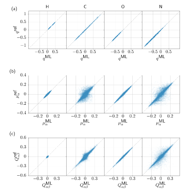
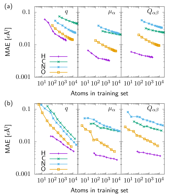
Fig. 2 display learning curves for the different multipole moments of each chemical element. It compares the two representations considered in this work: (a) Coulomb matrix and (b) aSLATM. The latter performs significantly better for point charges. Though we reach excellent accuracy for the monopoles, some of the higher multipoles remain more difficult, namely C and N. On the other hand, H and O both display excellent accuracy. The main difference between these two types of elements lies in their valency: H and O are often found as terminal atoms, while N and C display much more complex local environments. This likely affects the performance of the basis-set projection used in this work. The similar learning efficiency between the Coulomb matrix and aSLATM for dipoles and quadrupoles further suggests the need for larger training sets (e.g., Faber et al., went up to 120,000 samplesFaber et al. (2017)) or better local projections. We note the existence of ML methodologies that explicitly deal with tensorial objects, though only applied to dipoles so far.Glielmo, Sollich, and De Vita (2017); Grisafi et al. (2017) In Appendix B, we extend Glielmo et al.’s covariant-kernel description to quadrupoles using atom-centered Gaussian functions. Tests on small training sets indicated results on par with Fig. 2. We suspect that while covariant kernels offer a more robust description of the rotational properties of tensorial objects, the Coulomb matrix and aSLATM offer more effective representations, offsetting overall the results. Further, the construction of covariant kernels is computationally involved: it requires several outer products of rotation matrices to construct a $9\times 9$ matrix (Eqns. B and B) for a quadrupole alone. This significant computational overhead led us to use aSLATM with the basis-set projection for the rest of this work. Covariant kernels for multipoles up to quadrupoles are nonetheless implemented in our Python-based software.

Figure 2: ML of the multipole coefficients of neutral molecules. Comparison of representations: (a) Coulomb matrix and (b) aSLATM. Saturation curves of the mean-absolute error (MAE) for monopoles, dipoles, and quadrupoles of each chemical element.

III.2 Training of valence atomic densities

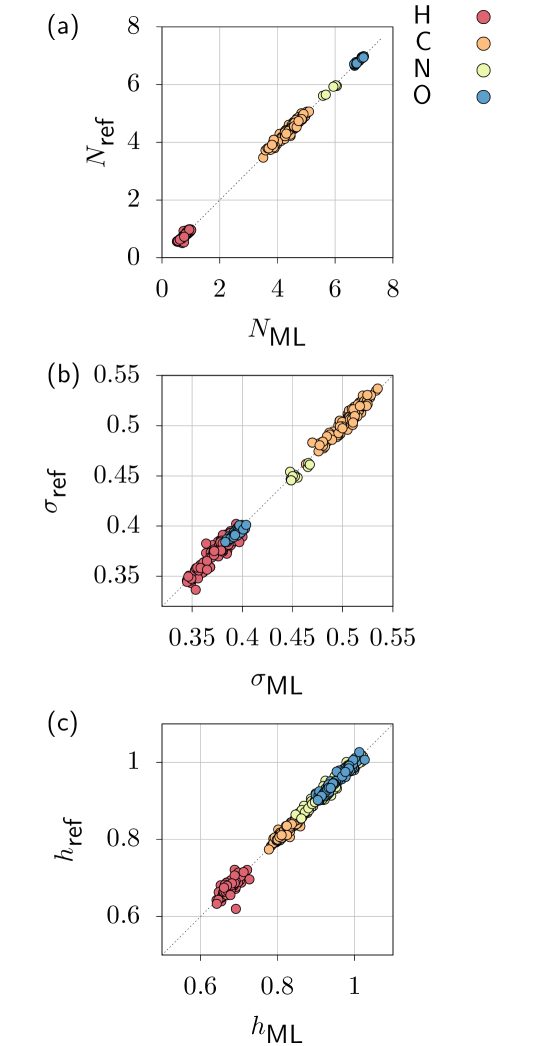
The accuracy of prediction of the populations and decay rates of valence atomic densities, $N$ and $\sigma$, respectively, for a size of the Coulomb matrix $n=6$ is shown on Fig. 3a and b. The model was trained against 13,500 atoms in 800 molecules, and tested against a separate set of 3,400 atoms in 200 molecules. The model shows high accuracy with MAEs of only 0.04 $e$ and 0.004 ${\rm a.u.}^{-1}$, respectively. Both models yield correlation coefficients above 99.5%.

III.3 Training of Hirshfeld ratios

Fig. 3c shows a correlation plot of the predicted and reference Hirshfeld ratios using the $n=12$ (i.e., size of the Coulomb matrix) model trained against 12,300 atoms in 1,000 small organic molecules. We test the prediction accuracy on a different set of 17,100 atoms. We find high correlation (coefficient of determination $R^{2}=99.5\%$) and a small MAE: 0.006.

Figure 3: Correlation plots of out-of-sample predictions. (a) ML of the populations (i.e., volume integral) of the valence atomic densities, $N$ (units in $e$). (b) ML of the decay rate of the valence atomic densities, $\sigma$ (units in ${\rm a.u.}^{-1}$). (c) ML of the Hirshfeld ratios, $h$.

III.4 Molecular polarizabilities

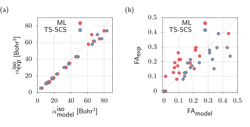
Predictions of the Hirshfeld ratios were further assessed by calculating (anisotropic) molecular polarizabilities. Reference experimental values of 18 small molecules were taken from Thole,Thole (1981) for both the isotropic molecular polarizability as well as the fractional anisotropy, as defined elsewhere.Bereau and von Lilienfeld (2014) Fig. 4 shows both the isotropic (panel a) and fractional anisotropy (panel b), comparing the present ML prediction with calculations using the Tkatchenko-Scheffler method after solving the self-consistent screening (SCS) equation.Tkatchenko and Scheffler (2009); DiStasio Jr, Gobre, and Tkatchenko (2014) We find excellent agreement between the ML prediction and experiment for the isotropic component: an MAE of $3.2$ Bohr³ and a mean-absolute relative error (MARE) of 8.6%, both virtually identical to the Tkatchenko-Scheffler calculations after SCS.DiStasio Jr, Gobre, and Tkatchenko (2014) The fractional anisotropy tends to be underestimated, though overall the agreement with experiment is reasonable, as compared to previous calculations that explicitly relied on DFT calculations for each compound.

Figure 4: Correlation plot between (a) isotropic and (b) fractional anisotropies of molecular polarizabilities predicted from the current ML model (blue) and Tkatchenko-Scheffler polarizabilities after SCS procedureTkatchenko and Scheffler (2009); DiStasio Jr, Gobre, and Tkatchenko (2014) (red) against experimental values for the set of 18 compounds proposed in Ref. 45.

III.5 Parametrization of the intermolecular energies

To optimize the abovementioned free parameters, we aimed at reproducing the intermolecular energies of a representative set of molecular dimers. The collection of global parameters optimized during this work are reported in Tab. 1. The parameters, shown in Tab. 1, were optimized simultaneously using basin hoppingWales and Doye (1997); Wales (2003) to reproduce the total intermolecular energy from reference calculations. We also provide a rough estimate of the sensitivity of these parameters through the standard deviation of all models up to 20% above the identified global minimum. We introduce chemical-element-specific prefactors for the repulsion interaction. The repulsive interaction is thus scaled by the product of element specific prefactors for each atom pair. The apparent lack of dependence of the dispersion parameter $d$ led us to fix it to the value $d=3.92$.Bereau and von Lilienfeld (2014)

Interaction	Parameter	Model 1		Model 2
		value	sensitivity	value	sensitivity
Polarization	$a$	0.0187	0.09	0.0193	0.03
Dispersion	$\gamma$	0.9760	0.04	0.9772	0.04
	$\beta$	2.5628	0.08	2.2789	0.04
	$d$	3.92		3.92
Repulsion	$U^{\rm rep}_{\rm H}$	27.3853	1	23.5936	1
	$U^{\rm rep}_{\rm C}$	24.6054	0.5	24.0509	0.5
	$U^{\rm rep}_{\rm N}$	22.4496	0.6	21.4312	0.3
	$U^{\rm rep}_{\rm O}$	16.1705	0.8	16.0782	0.2

Table 1: Optimized global parameters determined from two different training sets. Model 1: Fitting to the S22x5 at distances 0.9x and 1.0x. Model 2: Fitting to the S22x5 at distance 1.0x and S12L. Parameters $U_{\rm X}$ correspond to the repulsion of chemical element X, expressed in (kcal/mol)^1/2. “Value” corresponds to the optimal parameter, while “sensitivity” reflects the standard deviation of parameters around (up to 20% above) the identified global minimum. Sensitivity is not provided for $d$ (see main text).

A better understanding of the variability of our global parameters led us to consider two sets of reference datasets for fitting, coined below model 1 and model 2. While model 1 only considers small-molecule dimers, model 2 also incorporates host-guest complexes. For both models we rely on the S22x5 small-molecule datasetJurečka et al. (2006); Gráfová et al. (2010) at the equilibrium distance (i.e., 1.0x distance factor). In addition, model 1 also considers configurations at the shorter distance factor 0.9x to help improve the description of the curvature of the potential energy landscape. Model 2, on the other hand, adds to S22x5 at 1.0x a series of host-guest complexes: the S12L database.Ambrosetti et al. (2014a) All the results presented below will be derived from model 1, unless otherwise indicated. The comparison with model 2 aims at showing ($i$) the robustness of the fit from the relatively low variability of global parameters (except possibly for $U_{\rm H}$) and ($ii$) an outlook toward modeling condensed-phase systems.

Figure 5: Correlation of intermolecular energies for S22x5. The different panels describe the interactions at specific distance factors (i.e., from 0.9x to 2.0x). Color coding corresponds to the compound ID—hydrogen bonding compounds correspond to low values while van der Waals compounds correspond to the larger values. The different diagonals bracket the $\pm 1$ kcal/mol area of accuracy.

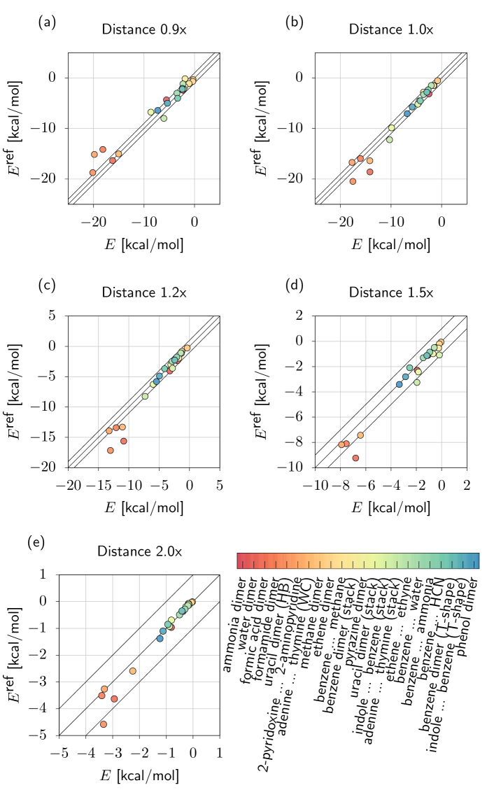
While the overall MAE averaged over all distance factors is 0.7 kcal/mol, the error clearly drops with distance: 1.0, 0.8, 0.8, 0.5, and 0.2 for distance factors 0.9x, 1.0x, 1.2x, 1.5x, and 2.0x, respectively. This illustrates that the model yields robust asymptotics, with significant improvement compared to a cruder model that only included multipole electrostatics and many-body dispersion.Bereau and von Lilienfeld (2014) Outliers from the $\pm 1~{}$kcal/mol accuracy region are composed of strongly hydrogen-bonding complexes (e.g., 2-pyridoxine with 2-aminopyridine), which depend significantly on the quality of the electrostatic description. The correlation achieved here depends critically on the accuracy of the multipole moments. Indeed, the few global parameters included in our model provide little room for error compensations. For instance, we found that a poorer ML model of the multipole moments yielded significant artifacts on the partial charges of hydrogen cyanide, leading to an artificially strong polarization of the hydrogen.

We also point out the small value of the polarization parameter, $a$ (Tab. 1), leading effectively to small polarization energies. Rather than an imbalance in the model, we suspect that significant short-range polarization energy is absorbed in the repulsion terms. Indeed, several AIM- and physics-based force fields use the same overlap model to describe repulsion and short-range polarization.Van Vleet et al. (2016); Vandenbrande et al. (2017) Since we optimize all terms directly against the total energy rather than decompose each term, such cancellations may well occur. We also expect that including systems in which strong non-additive polarization effects would play a role in outweighing effective pairwise polarization. In addition, we note that the pairwise scheme is optimized per chemical element, while the Thole model is not.

IV Performance of the IPML model

IV.1 Non-equilibrium geometries (S66a8)

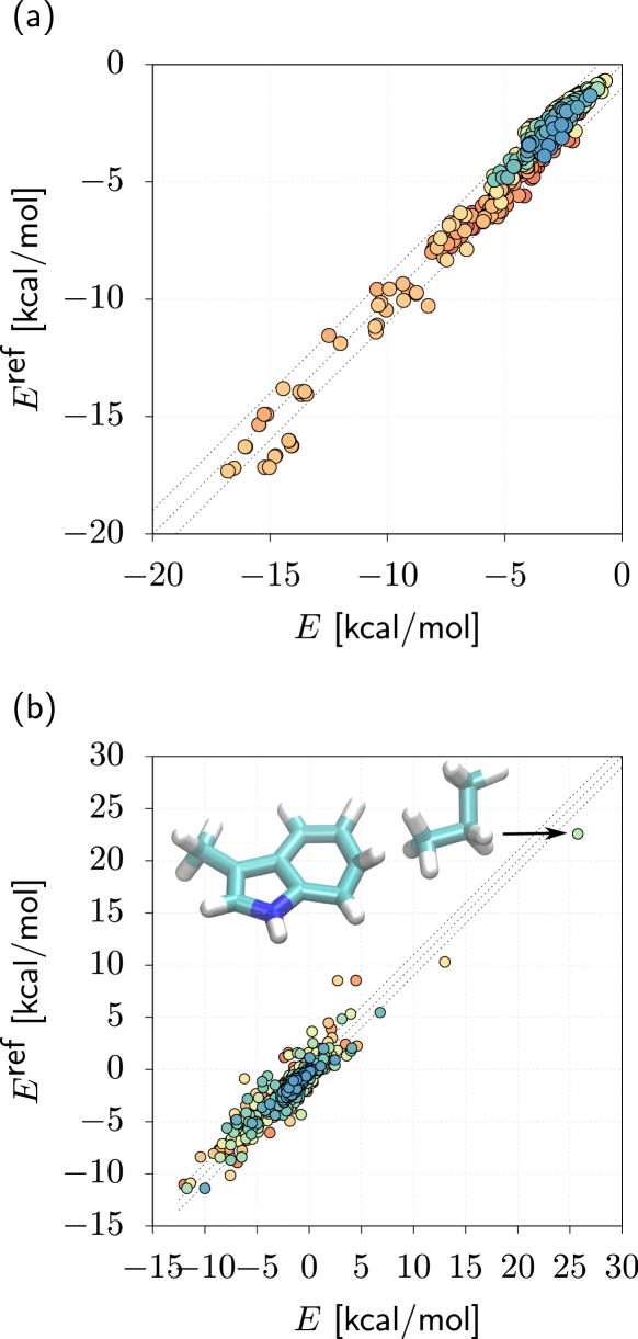
A recent extension of the S66 dataset of molecular dimers provides angular-displaced non-equilibrium geometries, i.e., S66a8 ($66\times 8=528$ dimers).Rezác, Riley, and Hobza (2011) The correlation between our model and reference calculations at the CCSD(T)/CBS level of theory are presented in Fig. 6a. Excellent agreement is found for most samples, with an MAE of only $0.4$ kcal/mol across a larger, representative set of molecular dimers, as compared to the S22 used for training. Model 2 performs virtually on par with an MAE of only $0.5$ kcal/mol.

Figure 6: Correlation plots for the total intermolecular energy between reference and present calculations for (a) the S66a8 dataset of dimers translated and rotated away from their equilibrium geometry and (b) the SSI dataset of amino acids (only dimers involving neutral compounds made of HCON atoms). Inset: strongly-repulsive tryptophan-glutamine dimer.

We compare our results with the MEDFF model whose overlap model is used in the present work, but relies on point-charge electrostatics and a pairwise dispersion model.Vandenbrande et al. (2017) They report root-mean squared errors of 0.36 kcal/mol for the dispersion-dominated complexes of the S66 dataset at equilibrium distances. Given that hydrogen-bonded complexes are typically more challenging,Grimme (2014); Vandenbrande et al. (2017) our model likely compares favorably, keeping in mind that the dataset and error measurement are different. They also report a reduced 0.26 kcal/mol error over the entire S66 dataset when each parameter is optimized specifically for each complex. Given our focus on model transferability, we did not attempt a similar measurement. For the same dataset and error measurement, the QMDFF model reports a larger 1.1 kcal/mol error.Vandenbrande et al. (2017)

IV.2 Amino-acid side chains (SSI dataset)

The SSI dataset contains pairs of amino-acid side chains extracted from the protein databank.Burns et al. (2017) We removed dimers containing charged compounds and sulfur-containing side chains (i.e., cysteine and methionine), for a total of 2,216 dimers. We computed intermolecular energies using the present method and compare them with reference CCSD(T) at the complete basis set limit. In Fig. 6b we compare the total energy with reference energies. We find again excellent agreement throughout the much larger range. We note the presence of a high-energy dimer at $+23$ kcal/mol, corresponding to a tryptophan-glutamine dimer (inset of Fig. 6b). The strong deformation of the tryptophan ring illustrates the robustness of our model in accurately reproducing intermolecular interactions for a variety of conformers. Model 1 yields overall an MAE of 0.37 kcal/mol. Interestingly, this accuracy is on par with additive force fields, such as GAFF and CGenFF (0.35 and 0.23 kcal/mol, respectively), and better than certain semi-empirical methods, e.g., AM1 (1.45 kcal/mol).Burns et al. (2017) Model 2 yields virtually the same MAE, 0.38 kcal/mol, but underpredicts the high-energy dimer highlighted in Fig. 6b: 3.6 instead of 22.6 kcal/mol. It highlights how widening the training set of the model to both small molecules and host-guest complexes decreases the accuracy on the former.

IV.3 DNA-base and amino-acid pairs (JSCH-2005)

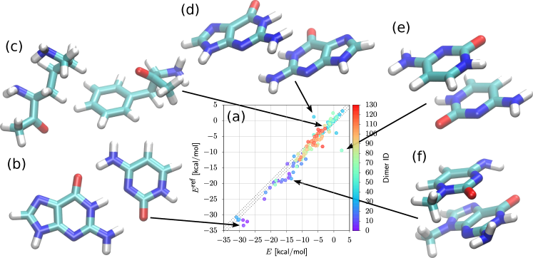
The JSCH-2005 dataset offers a benchmark of representative DNA base and amino-acid pairs.Jurečka et al. (2006) Again, we focus on neutral molecules only, for a total of 127 dimers. The correlation of total interaction energies is shown in Fig. 7a. We find a somewhat larger MAE of 1.4 kcal/mol. This result remains extremely encouraging, given the emphasis of strong hydrogen-bonded complexes present in this dataset. While others have pointed out the challenges associated with accurately modeling these interactions,Grimme (2014); Vandenbrande et al. (2017) we have not found reference benchmarks on specific datasets such as this one for similar physics-based models. Given the prevalence of hydrogen bonds in organic and biomolecular systems, we hope that this work will motivate a more systematic validation on these interactions.

Representative examples are shown on Fig. 7. While the Watson-Crick complex of the guanine (G) and cytosine (C) dimer (panel a) leads to one of the strongest binders, weak hydrogen bonds can still lead to the dominant contribution, as seen in (f) for the methylated GC complex. We find two outliers, shown in (d) and (e), where $\pi$-stacking interactions dominate the interaction energy. The discrepancies likely arise from an inadequate prediction of some quadrupole moments, especially involving nitrogen (see Fig. 1). Note the structural similarity between (d), (e), and (f): the weak hydrogen bonds in the latter case dominate the interaction and resolve any apparent discrepancy with the reference energy. For this dataset, model 2 performs significantly worse, with an MAE of $2.3$ kcal/mol, indicating that forcing transferability across both small-molecule dimers and host-guest complexes strains the accuracy of the model for challenging small molecules exhibiting significant $\pi$-stacking and hydrogen-bonding behavior. This significant change in performance contrasts the very similar parameters between the two models, highlighting a sensitive parameter dependence.

Figure 7: (a) Correlation plots for the total intermolecular energy between reference and present calculations for the JSCH-2005 datasetJurečka et al. (2006) of DNA-base and amino-acid pairs (dimers involving charged compounds are not shown). (b) GC in a Watson-Crick geometry; (c) Lysine and phenylalanine; (d) GG complex; (e) CC complex; (f) methylated GC complex.

IV.4 Water clusters

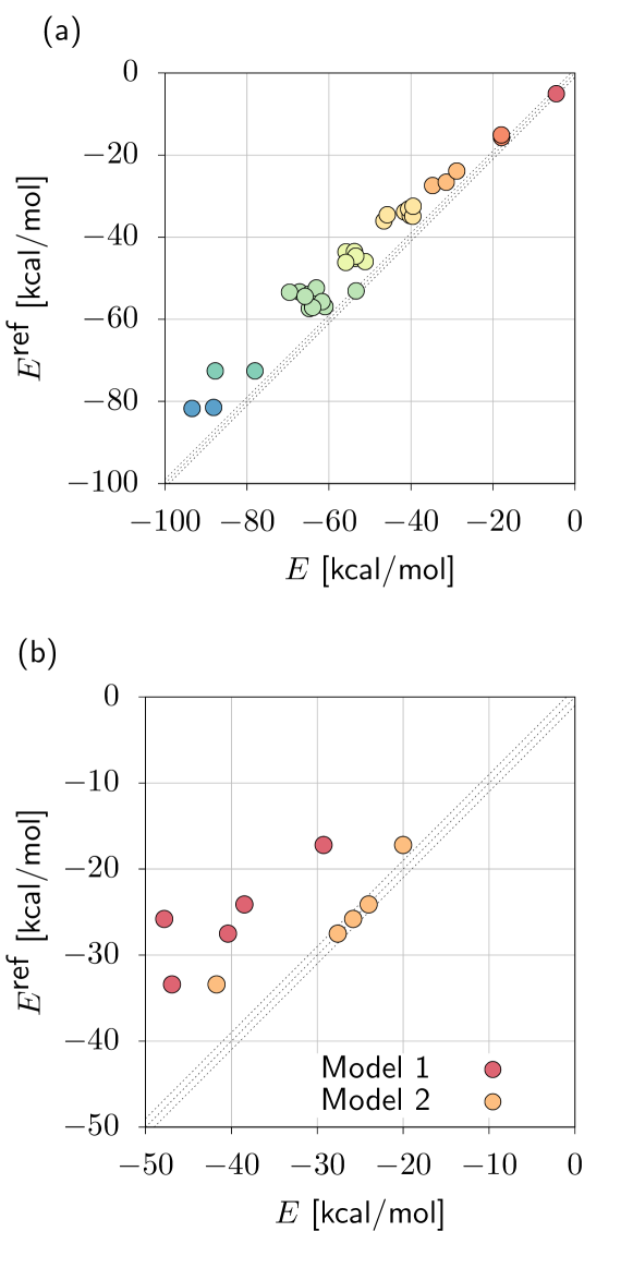
Beyond dimers, we test the ability of our potentials to reproduce energies of larger clusters. Fig. 8a shows the correlation of the total energy between the present work and CCSD(T) calculations at the complete basis set limit of water clusters involving from 2 to 10 molecules.Temelso, Archer, and Shields (2011) The model’s energies correlate highly with the reference but progressively overstabilize. This shift results from compounding errors that grow with cluster size, amounting to an MAE of 8.1 kcal/mol. Note that we can correct the slope by including a single water cluster in the above-mentioned parametrization (data not shown). Model 2 performs virtually on par with model 1.

IPML recovers the overall trend of energies for complexes of various sizes, but there is still room for improvements. This is notable given that the many-body polarization term was optimized to zero in both models (see Tab. 1). It indicates that a pairwise description captures the main effects even for the larger complexes considered here. Improving the results would require forcing the parametrization to rely more significantly on many-body polarization. Improving the modeling of other terms, such as repulsion, may also help reduce incidental cancellations of errors.

Figure 8: Correlation plots for the total intermolecular energy between reference and present calculations for (a) the water-clusters dataset and (b) the host-guest complexes in the S12L database. The colors in (a) indicate the number of molecules involved in the cluster: from two (red) to 10 (blue) molecules.

IV.5 Supramolecular complexes (S12L)

Moving toward more complex systems, we test the ability to reproduce intermolecular energies of host-guest complexes. Fig. 8b shows the correlation of the total intermolecular energy against diffusion Monte Carlo.Ambrosetti et al. (2014a) Although we find high correlation, the MAE is substantial: 9.7 kcal/mol. A comparison with model 2, which significantly improves the agreement, demonstrates the benefit of including larger complexes in the fit of the global parameters. Still, one outlier remains: the glycine anhydride-macrocycle, with an overstabilization of $8$ kcal/mol, despite being fitted into the global parameters. This compound (displayed in Fig. 8 of Ref. 32) displays sites at which multiple hydrogen bonds coincide. It further suggests the role of inaccurate multipoles, as well as an inadequate electrostatic penetration model (i.e., missing higher-order multipoles beyond monopole correction), and possibly many-body repulsion interactions.

IV.6 Benzene crystal

As another example leading to condensed-phase properties, we evaluate the model’s ability to reproduce the cohesive energy of the benzene crystal. We scale the lattice unit cell around the equilibrium value, as detailed in previous work.Bereau and von Lilienfeld (2014) The various contributions of the energy are shown in Fig. 9c. For reference, we compare the cohesive energy with experimental resultsSchweizer and Dunitz (2006) and dispersion-corrected atom-centered potentials (DCACP).Tapavicza et al. (2007)

Figure 9: Comparison of the intermolecular energy as a function of dimer distance for the benzene dimer in the (a) parallel-displaced and (b) T-shaped conformations. (c) Cohesive binding energy of the benzene crystal as a function of the scaling factor of the unit cell.

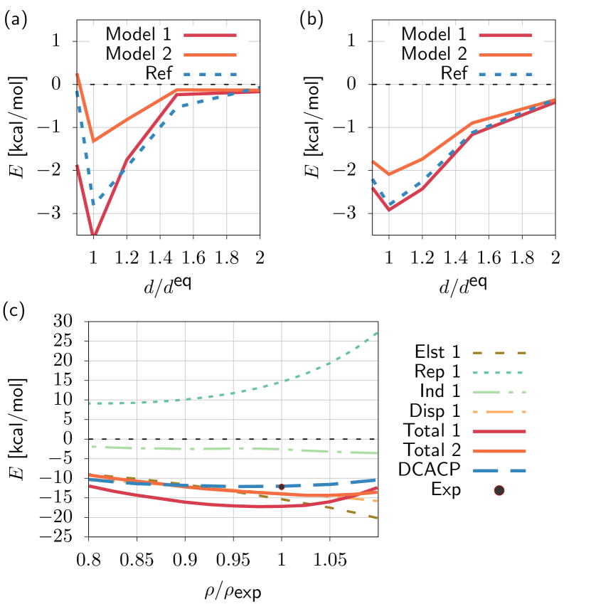
As reported before,von Lilienfeld and Tkatchenko (2010); Bereau and von Lilienfeld (2014) we find the benzene crystal to display significant dispersion interactions. Though the overall curvature against density changes agrees reasonably well with DCACP, we find that the method overstabilizes the molecular crystal. Model 1 yields a cohesive energy of $-17.2$ kcal/mol at equilibrium, as compared to the experimental value of $-12.2$ kcal/mol.Schweizer and Dunitz (2006) For reference, we show the potential energy landscapes of the benzene dimer in the stacked (a) and T-shaped (b) conformations. Excellent agreement is found in the latter case, while the former shows an overstabilization.

Interestingly, while model 2 seems to understabilize these two dimer configurations, it better reproduces the cohesive energy of the crystal, with a value at equilibrium density of $-14.3$ kcal/mol, only $2$ kcal/mol away from the experimental value. We conclude that the inclusion of host-guest complexes in the optimization of the global parameters helps describe systems toward or in the condensed phase. Still, the compounding errors present in the model limit a systematic extension to molecular crystals. We again point at the necessity for extremely accurate multipole moments, where any discrepancy can have significant effects in the condensed phase. Further improving the prediction of the multipole moments will strongly contribute to an improved accuracy of the present energy model.

V Conclusions and future outlook

We have presented a set of classical potentials to describe the intermolecular interactions of small molecules, coined IPML. Notably, we present a methodology that readily provides parameters for a large range of small molecules by relying on atom-in-molecule properties predicted from machine learning (ML). Predictions for distributed multipoles, Hirshfeld ratios, valence atomic density decay rate and population provide the necessary parameters for electrostatics, polarization, repulsion, and many-body dispersion. Remarkably, our methodology provides a first attempt at transferable intermolecular potentials with few global parameters optimized across a subset of chemical space containing H, C, N, and O atoms only. In contrast to other studies, we do not reoptimize the global parameters for every new compound. We rationalize this by the use of more sophisticated physical models, e.g., many-body rather than pairwise dispersion, multipole rather than point-charge electrostatics, and non-additive rather than pairwise additive polarization.

As compared to purely data-driven methodologies, IPML starts from physics-based interactions and only relies on ML to predict parameters thereof. Perturbation theory and the short-range overlap method offer an appealing framework to describe interactions based on monomer properties—effectively simplifying greatly the training of ML models of parameters. Conceptually, blending physical constraints in a data-driven framework would ideally translate into setting the functional form of the interaction as a prior of the ML model. As an example, reproducing kernel Hilbert space can fit a potential energy surface by imposing the asymptotics at long range.Ho and Rabitz (1996); Unke and Meuwly (2017)

Extensions of the present work to a force field would amount to computing derivatives. Analytical derivatives of the potentials with respect to atomic coordinates are either straightforward (e.g., pairwise repulsion and charge penetration) or already available (e.g., many-body dispersionBlood-Forsythe et al. (2016) or electrostatics and inductionPonder et al. (2010)). Our ML models being conformationally dependent, computation of the forces would also entail a derivative with respect to the atom-in-molecule properties. While not implemented here, this information can readily be extracted from derivatives of the kernel used in the ML.Rasmussen and Williams (2006) How to optimize such a conformationally-dependent force field to best balance the extra accuracy with the additional computational overhead remains an open problem.

Even though we did not aim at a performance optimization, the present implementation can help us gain insight into the computational cost of each term. Compared to standard classical force fields, the inclusion of explicit polarization and many-body dispersion leads to larger evaluation times: $1-100$ s for systems composed of $10-100$ atoms on a single core, respectively. Notably, roughly 90% of this time is spent predicting the multipoles, due to the large training set and complexity of the aSLATM representation. While such an evaluation time is significant, several strategies may be devised in the context of a molecular dynamics simulation. For instance, multipoles may remain frozen and only get updated when large conformational changes are detected.

We presented electrostatic calculations using distributed multipole—up to quadrupole—models. In comparison with other atomic properties, an accurate prediction of multipole electrostatics proves all the more challenging, and critical for the accurate estimation of various molecular systems. Improvements will require more accurate models, and possibly the incorporation of more advanced physical interactions, such as anisotropicVan Vleet, Misquitta, and Schmidt (2017) or many-body repulsion interactions. Our framework paves the way toward significantly more transferable models that blend in the physical laws and symmetries relevant for the phenomena at hand with a data-driven approach to infer the variation of environmentally-dependent local atomic parameters across chemical space. We expect such models that are transferable across chemical composition to be of use in systems of interest in chemistry, biology, and materials science.

Appendix A Many-body dispersion

The following summarizes the many-body dispersion (MBD) interactionTkatchenko and Scheffler (2009); Tkatchenko et al. (2012); Hermann, DiStasio Jr, and Tkatchenko (2017) as implemented elsewhere.Bereau and von Lilienfeld (2014) We recall the atomic polarizability $\alpha_{p}$ of atom $p$. The frequency dependence of $\alpha_{p}$ allows for an estimation of the pairwise dispersion coefficient via the Casimir-Polder integral

$$C_{6pq}=\frac{3}{\pi}\int_{0}^{\infty}{\rm d}\omega\alpha_{p}(i\omega)\alpha_{q}(i\omega),$$ (13)

where $i\omega$ are imaginary frequencies and $p$ and $q$ are a pair of atoms. Given reference free-atom values for $C_{6pp}$, we can estimate the characteristic frequency of atom $p$ $\omega_{p}=4C_{6pp}/3\alpha_{p}^{2}$.Chu and Dalgarno (2004)

The atomic polarizabilities and characteristic frequencies yield the necessary ingredients for the system of coupled quantum harmonic oscillators with $N$ atoms

$$C_{pq}^{\rm QHO}=\omega_{p}^{2}\delta_{pq}+(1-\delta_{pq})\omega_{p}\omega_{q}\sqrt{\alpha_{p}\alpha_{q}}\mathcal{T}_{pq},$$ (14)

where $\mathcal{T}_{pq}=\nabla_{{\bf r}_{p}}\otimes\nabla_{{\bf r}_{q}}W(r_{pq})$ is a dipole interaction tensor with modified Coulomb potential

$$W(r_{pq})=\frac{1-\exp{\left[-\left(\frac{r_{pq}}{R_{pq}^{\rm vdW}}\right)^{\beta}\right]}}{r_{pq}}.$$ (15)

In this equation, $\beta$ is a range-separation parameter and $R_{pq}^{\rm vdW}=\gamma(R_{p}^{\rm vdW}+R_{q}^{\rm vdW})$ is the sum of effective van der Waals radii scaled by a chemistry-independent fitting parameter. The effective van der Waals radius is obtained by scaling its reference free-atom counterpart: $R_{p}^{\rm vdW}=(\alpha_{p}/\alpha_{p}^{\rm free})^{1/3}R_{p}^{\rm vdW,free}$. An expression for $\mathcal{T}_{pq}$ is provided in Bereau et al.Bereau and von Lilienfeld (2014) In particular, we apply a range separation to the dipole interaction tensor by scaling it by a Fermi functionAmbrosetti et al. (2014b)

$$f(r_{pq})=\frac{1}{1+\exp{\left[-d(r_{pq}/R_{pq}^{\rm vdW}-1)\right]}}.$$ (16)

Diagonalizing the $3N\times 3N$ matrix $C_{pq}^{\rm QHO}$ yields its eigenvalues $\{\lambda_{i}\}$, which in turn provide the MBD energy

$$E_{\rm MBD}=\frac{1}{2}\sum_{i=1}^{3N}\sqrt{\lambda_{i}}-\frac{3}{2}\sum_{p=1}^{N}\omega_{p}.$$ (17)

The methodology depends on three chemistry-independent parameters: $\beta$, $\gamma$, and $d$.

Appendix B Covariant kernels

Glielmo et al.Glielmo, Sollich, and De Vita (2017) recently proposed a covariant kernel ${\bf K}^{\mu}$ for vector quantities—suitable here to predict dipoles—such that two samples $\rho$ and $\rho^{\prime}$ subject to rotations $\mathcal{S}$ and $\mathcal{S}^{\prime}$, respectively, will obey

$${\bf K}^{\mu}(\mathcal{S}\rho,\mathcal{S}^{\prime}\rho^{\prime})={\bf SK}^{\mu}(\rho,\rho^{\prime}){\bf S}^{\prime\rm T}.$$ (18)

The atom $i$ from sample $\rho$ is encoded by a set of atom-centered Gaussian functions

$$\rho({\bf r},\{{\bf r}_{i}\})=\frac{1}{(2\pi\sigma^{2})^{3/2}}\sum_{i}\exp\left(-\frac{||{\bf r}-{\bf r}_{i}||^{2}}{2\sigma^{2}}\right),$$ (19)

and the covariant kernel is analytically integrated over all 3D rotations to yieldGlielmo, Sollich, and De Vita (2017)

$${\bf K}^{\mu}(\rho,\rho^{\prime})=\frac{1}{L}\sum_{ij}\phi(r_{i},r_{j}){\bf r}_{i}\otimes{\bf r}_{j}^{\prime\rm T},$$ (20)

$$\phi(r_{i},r_{j})=\frac{\exp\left(-\alpha_{ij}\right)}{\gamma_{ij}^{2}}\left(\gamma_{ij}\cosh\gamma_{ij}-\sinh\gamma_{ij}\right),$$

$$L=(2\sqrt{\pi\sigma^{2}})^{3},\quad\alpha_{ij}=\frac{r_{i}^{2}+r_{j}^{2}}{4\sigma^{2}},\quad\gamma_{ij}=\frac{r_{i}r_{j}}{2\sigma^{2}},$$

where $\otimes$ denotes the outer product.

In the present work, we extend the construction of covariant kernels to predict quadrupole moments. Following a similar procedure adapted to second-rank tensors, we enforce the relation

$${\bf K}^{\rm Q}(\mathcal{S}\rho,\mathcal{S}^{\prime}\rho^{\prime})={\bf S}^{\prime}{\bf S}^{\rm T}{\bf K}^{\rm Q}(\rho,\rho^{\prime}){\bf S}{\bf S}^{\prime\rm T}$$ (21)

onto a base pairwise kernel of diagonal form: ${\bf K}^{\rm b}(\rho,\rho^{\prime})=\mathbb{1}k^{\rm b}(\rho,\rho^{\prime})$, where $k^{\rm b}(\rho,\rho^{\prime})$ is independent of the reference frame. The covariant kernel is constructed by integrating the base kernel over all 3D rotations

$${\bf K}^{\rm Q}(\rho,\rho^{\prime})=\frac{1}{L}\sum_{ij}\int{\rm d}\mathcal{S}{\bf S}\otimes{\bf S}^{\rm T}k^{\rm b}(\rho,\mathcal{S}^{\rm T}\rho^{\prime}),$$ (22)

which leads to the expression

$${\bf K}^{\rm Q}(\rho,\rho^{\prime})=\frac{1}{L}\sum_{ij}\left({\bf R}_{j}^{\rm T}\otimes{\bf R}_{i}\right)\Phi(r_{i},r_{j})\left({{\bf R}_{i}}^{\rm T}\otimes{\bf R}_{j}\right),$$

$$\Phi(r_{i},r_{j})=\int{\rm d}\mathcal{\tilde{R}}\tilde{\bf R}^{\rm T}\otimes\tilde{\bf R}k^{\rm b}(\tilde{\bf r}_{i},\tilde{\bf R}\tilde{\bf r}^{\prime}_{j}),$$ (23)

where ${\bf R}_{i}$ and ${\bf R}_{j}$ are the rotation matrices that align ${\bf r}_{i}$ and ${\bf r}_{j}$ onto the $z$ axis to form $\tilde{\bf r}_{i}$ and $\tilde{\bf r}^{\prime}_{j}$, respectively.Glielmo, Sollich, and De Vita (2017) We analytically integrate all 3D rotations

$$\Phi(r_{i},r_{j})= {\rm e}^{\frac{-\alpha_{ij}^{2}}{4\sigma^{2}}}\int{\rm d}\alpha\int{\rm d}\beta\int{\rm d}\gamma\frac{\sin\beta}{8\pi^{2}}$$

$$\times{\bf R}^{\rm T}(\alpha,\beta,\gamma)\otimes{\bf R}(\alpha,\beta,\gamma){\rm e}^{\frac{r_{i}r_{j}\cos\beta}{2\sigma^{2}}}$$

$$= \left(\begin{array}[]{ccccccccc}\varphi_{1}&0&0&0&\varphi_{2}&0&0&0&0\\ 0&\varphi_{1}&0&-\varphi_{2}&0&0&0&0&0\\ 0&0&\varphi_{3}&0&0&0&0&0&0\\ 0&-\varphi_{2}&0&\varphi_{1}&0&0&0&0&0\\ \varphi_{2}&0&0&0&\varphi_{1}&0&0&0&0\\ 0&0&0&0&0&\varphi_{3}&0&0&0\\ 0&0&0&0&0&0&\varphi_{3}&0&0\\ 0&0&0&0&0&0&0&\varphi_{3}&0\\ 0&0&0&0&0&0&0&0&\varphi_{4}\\ \end{array}\right),$$ (33)

where

$$\varphi_{1} =\frac{{\rm e}^{\frac{-\alpha_{ij}^{2}}{4\sigma^{2}}}}{4\gamma_{ij}^{2}}\left(\gamma^{2}_{ij}\sinh\gamma_{ij}-\gamma_{ij}\cosh\gamma_{ij}+\sinh\gamma_{ij}\right)$$

$$\varphi_{2} =\frac{{\rm e}^{\frac{-\alpha_{ij}^{2}}{4\sigma^{2}}}}{4\gamma_{ij}}\left(\gamma_{ij}\cosh\gamma_{ij}-\sinh\gamma_{ij}\right)$$

$$\varphi_{3} =\frac{{\rm e}^{\frac{-\alpha_{ij}^{2}}{4\sigma^{2}}}}{2\gamma_{ij}^{2}}\left(\gamma_{ij}\cosh\gamma_{ij}-\sinh\gamma_{ij}\right)$$

$$\varphi_{4} =\frac{{\rm e}^{\frac{-\alpha_{ij}^{2}}{4\sigma^{2}}}}{\gamma_{ij}^{2}}\left(\frac{\gamma^{2}_{ij}}{2}\sinh\gamma_{ij}-\gamma_{ij}\cosh\gamma_{ij}+\sinh\gamma_{ij}\right).$$ (34)

References

- Grimme (2014) S. Grimme, J. Chem. Theory Comput. 10, 4497 (2014).
- Metz, Piszczatowski, and Szalewicz (2016) M. P. Metz, K. Piszczatowski, and K. Szalewicz, J. Chem. Theory Comput. 12, 5895 (2016).
- Jeziorski, Moszynski, and Szalewicz (1994) B. Jeziorski, R. Moszynski, and K. Szalewicz, Chem. Rev. 94, 1887 (1994).
- Van Vleet et al. (2016) M. J. Van Vleet, A. J. Misquitta, A. J. Stone, and J. Schmidt, J. Chem. Theory Comput. 12, 3851 (2016).
- Vandenbrande et al. (2017) S. Vandenbrande, M. Waroquier, V. V. Speybroeck, and T. Verstraelen, J. Chem. Theory Comput. 13, 161 (2017).
- Cole et al. (2016) D. J. Cole, J. Z. Vilseck, J. Tirado-Rives, M. C. Payne, and W. L. Jorgensen, J. Chem. Theory Comput. 12, 2312 (2016).
- Bartók et al. (2010) A. P. Bartók, M. C. Payne, R. Kondor, and G. Csányi, Phys. Rev. Lett. 104, 136403 (2010).
- Li, Kermode, and De Vita (2015) Z. Li, J. R. Kermode, and A. De Vita, Phys. Rev. Lett. 114, 096405 (2015).
- Behler (2016) J. Behler, J. Chem. Phys. 145, 170901 (2016).
- Chmiela et al. (2017) S. Chmiela, A. Tkatchenko, H. E. Sauceda, I. Poltavsky, K. T. Schütt, and K.-R. Müller, Sci. Adv. 3, e1603015 (2017).
- Botu et al. (2016) V. Botu, R. Batra, J. Chapman, and R. Ramprasad, J. Phys. Chem. C 121, 511 (2016).
- Schütt et al. (2017) K. T. Schütt, F. Arbabzadah, S. Chmiela, K. R. Müller, and A. Tkatchenko, Nat. Comm. 8, 13890 (2017).
- Natarajan, Morawietz, and Behler (2015) S. K. Natarajan, T. Morawietz, and J. Behler, Phys. Chem. Chem. Phys. 17, 8356 (2015).
- Rupp et al. (2012) M. Rupp, A. Tkatchenko, K.-R. Müller, and O. A. Von Lilienfeld, Phys. Rev. Lett. 108, 058301 (2012).
- Hansen et al. (2013) K. Hansen, G. Montavon, F. Biegler, S. Fazli, M. Rupp, M. Scheffler, O. A. Von Lilienfeld, A. Tkatchenko, and K.-R. Müller, J. Chem. Theory Comput. 9, 3404 (2013).
- Ramakrishnan and von Lilienfeld (2017) R. Ramakrishnan and O. A. von Lilienfeld, “Machine learning, quantum chemistry, and chemical space,” in Rev. Comp. Ch. (John Wiley & Sons, Inc., 2017) pp. 225–256.
- Bereau and Kremer (2015) T. Bereau and K. Kremer, J. Chem. Theory Comput. 11, 2783 (2015).
- Bereau, Andrienko, and von Lilienfeld (2015) T. Bereau, D. Andrienko, and O. A. von Lilienfeld, J. Chem. Theory Comput. 11, 3225 (2015).
- Stone (2013) A. Stone, The theory of intermolecular forces (Oxford University Press, 2013).
- Jurečka et al. (2006) P. Jurečka, J. Šponer, J. Černỳ, and P. Hobza, Phys. Chem. Chem. Phys. 8, 1985 (2006).
- Zhao and Truhlar (2008) Y. Zhao and D. G. Truhlar, Theor. Chem. Acc. 120, 215 (2008).
- Misquitta, Stone, and Fazeli (2014) A. J. Misquitta, A. J. Stone, and F. Fazeli, J. Chem. Theory Comput. 10, 5405 (2014).
- (23) T. Verstraelen, P. Tecmer, F. Heidar-Zadeh, K. Boguslawski, M. Chan, Y. Zhao, T. D. Kim, S. Vandenbrande, D. Yang, C. E. González-Espinoza, S. Fias, P. A. Limacher, D. Berrocal, A. Malek, and P. W. Ayers, “HORTON, version 2.0.1,” http://theochem.github.com/horton/, accessed: 2016-08-01.
- Huang and von Lilienfeld (2016) B. Huang and O. A. von Lilienfeld, J. Chem. Phys. 145, 161102 (2016).
- Huang and von Lilienfeld (2017) B. Huang and O. A. von Lilienfeld, arXiv preprint arXiv:1707.04146 (2017).
- (26) A. S. Christensen, F. A. Faber, B. Huang, L. A. Bratholm, A. Tkatchenko, K. R. Müller, and O. A. von Lilienfeld, “QML: A Python Toolkit for Quantum Machine Learning,” https://github.com/qmlcode/qml, accessed: 2017-07-01.
- Kim, Kim, and Lee (1981) Y. S. Kim, S. K. Kim, and W. D. Lee, Chem. Phys. Lett. 80, 574 (1981).
- Lillestolen and Wheatley (2008) T. C. Lillestolen and R. J. Wheatley, Chem. Commun. 45, 5909 (2008).
- Verstraelen et al. (2016) T. Verstraelen, S. Vandenbrande, F. Heidar-Zadeh, L. Vanduyfhuys, V. Van Speybroeck, M. Waroquier, and P. W. Ayers, J. Chem. Theory Comput. 12, 3894 (2016).
- Hirshfeld (1977) F. L. Hirshfeld, Theor. Chim. Acta 44, 129 (1977).
- Tkatchenko and Scheffler (2009) A. Tkatchenko and M. Scheffler, Phys. Rev. Lett. 102, 073005 (2009).
- Bereau and von Lilienfeld (2014) T. Bereau and O. A. von Lilienfeld, J. Chem. Phys. 141, 034101 (2014).
- Bučko et al. (2014) T. Bučko, S. Lebègue, J. G. Ángyán, and J. Hafner, J. Chem. Phys. 141, 034114 (2014).
- Gobre (2016) V. V. Gobre, Efficient modelling of linear electronic polarization in materials using atomic response functions, Ph.D. thesis, Technische Universität Berlin (2016).
- Adamo and Barone (1999) C. Adamo and V. Barone, J. Chem. Phys. 110, 6158 (1999).
- Kannemann and Becke (2010) F. O. Kannemann and A. D. Becke, J. Chem. Theory Comput. 6, 1081 (2010).
- Otero-de-la Roza and Johnson (2013) A. Otero-de-la Roza and E. R. Johnson, J. Chem. Phys. 138, 054103 (2013).
- Ren and Ponder (2003) P. Ren and J. W. Ponder, J. Phys. Chem. B 107, 5933 (2003).
- Bereau, Kramer, and Meuwly (2013) T. Bereau, C. Kramer, and M. Meuwly, J. Chem. Theory Comput. 9, 5450 (2013).
- Wang and Truhlar (2010) B. Wang and D. G. Truhlar, J. Chem. Theory Comput. 6, 3330 (2010).
- Piquemal, Gresh, and Giessner-Prettre (2003) J.-P. Piquemal, N. Gresh, and C. Giessner-Prettre, J. Phys. Chem. A 107, 10353 (2003).
- Wang et al. (2015) Q. Wang, J. A. Rackers, C. He, R. Qi, C. Narth, L. Lagardere, N. Gresh, J. W. Ponder, J.-P. Piquemal, and P. Ren, J. Chem. Theory Comput. 11, 2609 (2015).
- Narth et al. (2016) C. Narth, L. Lagardère, E. Polack, N. Gresh, Q. Wang, D. R. Bell, J. A. Rackers, J. W. Ponder, P. Y. Ren, and J.-P. Piquemal, J. Comput. Chem. 37, 494 (2016).
- Rackers et al. (2017) J. A. Rackers, Q. Wang, C. Liu, J.-P. Piquemal, P. Ren, and J. W. Ponder, Phys. Chem. Chem. Phys. 19, 276 (2017).
- Thole (1981) B. T. Thole, Chem. Phys. 59, 341 (1981).
- Hermann, DiStasio Jr, and Tkatchenko (2017) J. Hermann, R. A. DiStasio Jr, and A. Tkatchenko, Chem. Rev 117, 4714 (2017).
- Tkatchenko et al. (2012) A. Tkatchenko, R. A. DiStasio Jr, R. Car, and M. Scheffler, Phys. Rev. Lett. 108, 236402 (2012).
- Donchev (2006) A. Donchev, J. Chem. Phys. 125, 074713 (2006).
- van der Walt, Colbert, and Varoquaux (2011) S. van der Walt, S. C. Colbert, and G. Varoquaux, Computing in Science & Engineering 13, 22 (2011).
- O’Boyle et al. (2011) N. M. O’Boyle, M. Banck, C. A. James, C. Morley, T. Vandermeersch, and G. R. Hutchison, J. Cheminform. 3, 33 (2011).
- Faber et al. (2017) F. A. Faber, L. Hutchison, B. Huang, J. Gilmer, S. S. Schoenholz, G. E. Dahl, O. Vinyals, S. Kearnes, P. F. Riley, and O. A. von Lilienfeld, J. Chem. Theory Comput. 13, 5255 (2017).
- Glielmo, Sollich, and De Vita (2017) A. Glielmo, P. Sollich, and A. De Vita, Phys. Rev. B 95, 214302 (2017).
- Grisafi et al. (2017) A. Grisafi, D. M. Wilkins, G. Csányi, and M. Ceriotti, arXiv preprint arXiv:1709.06757 (2017).
- DiStasio Jr, Gobre, and Tkatchenko (2014) R. A. DiStasio Jr, V. V. Gobre, and A. Tkatchenko, J. Phys.: Condens. Matter 26, 213202 (2014).
- Wales and Doye (1997) D. J. Wales and J. P. Doye, J. Phys. Chem. A 101, 5111 (1997).
- Wales (2003) D. J. Wales, Energy landscapes: Applications to clusters, biomolecules and glasses (Cambridge University Press, 2003).
- Gráfová et al. (2010) L. Gráfová, M. Pitonak, J. Rezac, and P. Hobza, J. Chem. Theory Comput. 6, 2365 (2010).
- Ambrosetti et al. (2014a) A. Ambrosetti, D. Alfè, R. A. DiStasio Jr, and A. Tkatchenko, J. Phys. Chem. Lett. 5, 849 (2014a).
- Rezác, Riley, and Hobza (2011) J. Rezác, K. E. Riley, and P. Hobza, J. Chem. Theory Comput. 7, 3466 (2011).
- Burns et al. (2017) L. A. Burns, J. C. Faver, Z. Zheng, M. S. Marshall, D. G. A. Smith, K. Vanommeslaeghe, A. D. MacKerell Jr., K. M. Merz Jr., and D. Sherrill, J. Chem. Phys. 147, 161727 (2017).
- Temelso, Archer, and Shields (2011) B. Temelso, K. A. Archer, and G. C. Shields, J. Phys. Chem. A 115, 12034 (2011).
- Schweizer and Dunitz (2006) W. B. Schweizer and J. D. Dunitz, J. Chem. Theory Comput. 2, 288 (2006).
- Tapavicza et al. (2007) E. Tapavicza, I.-C. Lin, O. A. von Lilienfeld, I. Tavernelli, M. D. Coutinho-Neto, and U. Rothlisberger, J. Chem. Theory Comput. 3, 1673 (2007).
- von Lilienfeld and Tkatchenko (2010) O. A. von Lilienfeld and A. Tkatchenko, J. Chem. Phys. 132, 234109 (2010).
- Ho and Rabitz (1996) T.-S. Ho and H. Rabitz, J. Chem. Phys. 104, 2584 (1996).
- Unke and Meuwly (2017) O. T. Unke and M. Meuwly, J. Chem. Inf. Model. 57, 1923 (2017).
- Blood-Forsythe et al. (2016) M. A. Blood-Forsythe, T. Markovich, R. A. DiStasio Jr, R. Car, and A. Aspuru-Guzik, Chem. Sci. 7, 1712 (2016).
- Ponder et al. (2010) J. W. Ponder, C. Wu, P. Ren, V. S. Pande, J. D. Chodera, M. J. Schnieders, I. Haque, D. L. Mobley, D. S. Lambrecht, R. A. DiStasio Jr, et al., J. Phys. Chem. B 114, 2549 (2010).
- Rasmussen and Williams (2006) C. E. Rasmussen and C. K. Williams, Gaussian processes for machine learning, Vol. 1 (MIT press Cambridge, 2006).
- Van Vleet, Misquitta, and Schmidt (2017) M. J. Van Vleet, A. J. Misquitta, and J. R. Schmidt, Journal of chemical theory and computation (2017), 10.1021/acs.jctc.7b00851.
- Chu and Dalgarno (2004) X. Chu and A. Dalgarno, J. Chem. Phys. 121, 4083 (2004).
- Ambrosetti et al. (2014b) A. Ambrosetti, A. M. Reilly, R. A. DiStasio Jr, and A. Tkatchenko, J. Chem. Phys. 140, 18A508 (2014b).