Particle Filtering for Stochastic Navier-Stokes Signal Observed with Linear Additive Noise
Abstract
We consider a non-linear filtering problem, whereby the signal obeys the stochastic Navier-Stokes equations and is observed through a linear mapping with additive noise. The setup is relevant to data assimilation for numerical weather prediction and climate modelling, where similar models are used for unknown ocean or wind velocities. We present a particle filtering methodology that uses likelihood informed importance proposals, adaptive tempering, and a small number of appropriate Markov Chain Monte Carlo steps. We provide a detailed design for each of these steps and show in our numerical examples that they are all crucial in terms of achieving good performance and efficiency.
1 Introduction
We focus on a stochastic filtering problem where a space and time varying hidden signal is observed at discrete times with noise. The non-linear filtering problem consists of computing the conditional probability law of the hidden stochastic process (the so-called signal) given observations of it collected in a sequential manner. In particular, we model the signal with a particular dissipative stochastic partial differential equation (SPDE), which is the stochastic Navier-Stokes Equation (NSE). This model, or a variant thereof, is often used in applications to model unknown quantities such as atmosphere or ocean velocity. In the spirit of data assimilation and uncertainty quantification, we wish to extract information for the trajectory of the hidden signal from noisy observations using a Bayesian approach. Typical applications include numerical weather forecasting in meteorology, oceanography and atmospheric sciences, geophysics, hydrology and petroleum engineering; see [2, 34, 5] for an overview.
We restrict to the setting where the state of interest is the time varying velocity field, , in some 2D bounded set . The unknown state is modelled using the stochastic NSE
| (1) |
where is the Laplacian, a viscosity constant, a non-linear operator due to convection, a positive, self adjoint, trace class operator, a determistic forcing and a space-time white noise as in [11]. This might appear as a restrictive choice for the dynamics, but the subsequent methodology is generic and could be potentially applied to other similar dissipative SPDEs, such as the stochastic Burger’s or Kuramoto–Sivashinski equations [24, 7].
The evolution of the unknown state of the SPDE is observed at discrete times and generates a sequence of noisy observations . In order to perform accurate estimation and uncertainty quantification, we are interested not just in approximating a single trajectory estimate of the hidden state, but in the complete filtering distribution,
| (2) |
that is, the conditional distribution of the state given all the observations obtained up to current time . The main objective is to compute the filtering distribution as it evolves with time, which is an instance of the stochastic filtering problem [1]. The solution of the problem can be formulated rigorously as a recursive Bayesian inference problem posed on an appropriate function space [31]. In contrast to standard filtering problems, the problem setup here is particularly challenging: the prior consists of a complicated probability law generated by the SPDE [11] and observation likelihoods on the high dimensional space of the signal tend to be very informative.
The aim of this paper is to propose Sequential Monte Carlo (SMC) methods (also known as Particle Filters (PF)) that can approximate effectively these conditional distributions. Computing the evolution of the filtering distribution is not analytically tractable, except in linear Gaussian settings. SMC is a generic Monte Carlo method that approximates the sequence of -s and their normalising constant (known in Statistics as marginal likelihood or evidence). This is achieved by obtaining samples known as particles and combining Importance Sampling (IS), resampling and parallel Markov Chain Monte Carlo (MCMC) steps. The main advantages of the methodology are: i) it is sequential and on-line in nature; ii) it does not require restrictive model assumptions such as Gaussian noise or linear dynamics and observations; iii) it is parallelisable, so one could gain significant speed-up using appropriate hardware (e.g. GPUs, computing clusters) [33]; iv) it is a well-studied principled method with an extensive literature justifying its validity and theoretical properties, see e.g. [13, 12]. So far SMC has been extremely successful in typically low to moderate dimensions [16], but its application in high dimensional settings has been very challenging mainly due to the difficulty to perform IS efficiently in high dimensions [41]. Despite this challenge a few successful high dimensional SMC implementations have appeared recently for applications with discrete time signal dynamics [36, 46, 45, 47, 5, 8, 3].
We will formulate the filtering problem with discrete time observations and continuous time dynamics. This setup has appeared previously in [40, 39] for signals corresponding to low dimensional stochastic differential equations (SDEs). The aim of this paper is to provide a novel, accurate and more efficient SMC design when the hidden signal is modelled by a SPDE with linear Gaussian observation. To achieve this challenging task, the particle filter will use computational tools that have been previously successful in similar high dimensional problems, such as tempering [29] and pre-conditioned Crank Nicholson MCMC steps [23, 9]. Using such tools, we propose a particle algorithm that can be used to approximate when the signal obeys the stochastic NSE and the observations are linear with additive noise. On a general level, the proposed algorithm has a similar structure to [27], but here we additionally adopt the use of IS. We will provide a detailed design of the necessary likehood informed importance proposals and the MCMC moves used. We extend known IS techniques for SDEs ([22, 48]) and MCMC moves for high dimensional problems ([43, 23, 9]) to make them applicable for filtering problems involving the stochastic NSE or other dissipative SPDEs. In the context of particle filtering, our developments leads to an SMC algorithm that performs effectively for the high dimensional problem at hand using a moderate amount of particles.
The material presented in this paper can be viewed as an extension of some ideas in the authors’ earlier work in [29]. In [29] we considered the deterministic NSE with more general observation equations. In the present paper the model for the signal contains additive noise and we assume linear observation schemes. This allows for the possibility of using likehood informed importance proposals and the MCMC steps need to be designed to be invariant to a more complicated conditional law due to the SPDE dynamics. The organisation of this paper is as follows: in Section 2 we present some background on the stochastic NSE and in Section 3 we formulate the filtering problem of interest. In Section 4 we present the SMC algorithm and in Section 5 we prsesent a numerical case study that illustrates the performance and efficiency of our method. Finally, in Section 6 we provide some concluding remarks.
2 Background on the Stochastic Navier-Stokes Equations
We present some background on the 2D stochastic NSE defined on an appropriate separable Hilbert space. We restrict the presentation to the case of periodic boundary conditions following the treatment in [18]. This choice is motivated mainly for convenience in exposition and for performing numerical approximations using Fast Fourier Transforms (FFT). The formulation and properties of the stochastic NSE can allow for the more technically demanding Dirichlet conditions on a smooth boundary [19, 23]. We stress that the subsequent particle filtering methodology is generic and does not rely on the choice of boundary conditions.
2.1 Preliminaries
Let the region of interest be the torus with being a point on the space. The quantity of interest is a time-space varying velocity field , and due to the periodic boundary conditions; here denotes vector/matrix transpose. It is convenient to work with the Fourier characterisation of the function space of interest:
| (3) |
using the following orthonormal basis functions for ,
The deterministic NSE is given by the following the functional evolution equation
| (4) |
Following standard notation we denote for the Leray projector ( is the space of squared-integrable periodic functions), for the Stokes operator, for the convection mapping and for the forcing.
One can introduce additive noise in the dynamics in a standard manner. First, we define the upper half-plane of wavenumbers
Let
where are (independent) standard Brownian motions on . In the spirit of [11, Section 4.1], consider a covariance operator such that , for , . Then, we can define the -Wiener process as
| (5) |
under the requirement , . Thus, we are working with a diagonal covariance matrix (w.r.t. the relevant basis of interest), though other choices could easily be considered. We will also work under the scenario that , for some , so that , i.e. is trace-class operator. Finally, we will use to denote the -Wiener measure on .
Having introduced the random component, we are now interested in weak solutions of the functional SDE,
| (6) |
with the solution understood pathwise on the probability space . More formally, following [18], we define the spaces
Since the operator is linear, bounded in and , [18, Theorem 6.1] implies that for and , there exists a unique solution for (6) such that . In [18, 19] one may also find more details on the existence of an invariant distribution, together with irreducibility and Feller properties of the corresponding Markov transition kernel.
2.2 Galerkin Projections and Computational Considerations
Using the Fourier basis (3), we can write the solution as
Hence, it is equivalent to consider the parameterisation of via . By taking the inner product with on both sides of (6), it is straightforward to obtain that the ’s obey the following infinite-dimensional SDE
| (7) |
with
Recall that due to being a real field , . This parameterisation of is more convenient as it allows performing inference on a vector (even if infinitely long), with coordinates evolving according to an SDE. For numerical purposes one is forced to use Galerkin discretisations, using projections of onto a finite Hilbert space instead. Consider the set of wavenumbers in
for some integer , and define the finite dimensional-subspace via the projection so that
Then, infering the Galerkin projection for corresponds to inferring the vector that obeys the following finite-dimensional SDE
| (8) |
This high dimensional SDE will provide an approximation for the infinite dimensional SPDE. Such an inference problem is more standard, but is still challenging due to the high dimensionality of and the non-linearities involved in the summation term of the drift function in (8). Since (8) is only an approximation of (7), it will induce a bias in the inferential procedure. In our paper, we do not study the size of this bias. Instead we concentrate our efforts on designing an algorithm to approximate (in (2)) that is robust to mesh refinement. This means our method should perform well numerically when one increases (and, indeed, reducing the bias in the numerical approximation of (7)). Naturally this would be at the expense of adding computational effort at a moderate amount, but this will depend on the particular numerical scheme used to approximate the solution of (8). For instance, for the FFT based numerical schemes used in Section 5 the computational cost is .
2.3 The Distribution of
We assume that the initial condition of is random and distributed according to the following Gaussian process prior:
| (9) |
with hyper-parameters affecting the roughness and magnitude of the initial vector field. This is a convenient but still flexible enough choice of a prior; see [11, Sections 2.3 and 4.1] for more details on Gaussian distributions on Hilbert spaces. Notice that admits the Karhunen-Loève expansion
with , , (so, necessarily , ) and
Since the covariance operator is determined via the Stokes operator , one can easily check that the choice implies that for , -a.s., thus the conditions for existence of weak solution of (6) in [18, Theorem 6.1] are satisfied a.s. in the initial condition. Notice that sampling from is straightforward.
3 The Stochastic Filtering Problem
In Section 2 we defined the SPDE providing the unknown signal, i.e. the object we are interested in performing Bayesian inference upon. In this section we present the non-linear filtering problem in detail. We begin by discussing the observations. We assume that the vector field is unknown, but generates a sequence of noisy observations at ordered discrete time instances with for all , with , for , Each observation vector is further assumed to originate from the following observation equation
| (10) |
where is a bounded linear operator and is symmetric positive-definite. One can then write the observation likelihood at instance as
Using a linear observation model is restrictive but it does include typical observation schemes used in practice. We focus our attention at the case when is a noisy measurement of the velocity field at different fixed stationary points , . This setting is often referred to as Eulerian data assimilation. In particular we have that
with denoting a spatial average over a (typically small) region around , , say for some radius ; that is, is the following integral operator
| (11) |
with denoting the area of . In what follows, other integral operators could also be similarly used, such as , with being appropriate weighting functions that decay as grows.
Earlier in the introduction, the filtering problem was defined as the task of computing the conditional distribution . Due to the nature of the observations, it is clear we are dealing with a discrete time filtering problem. A particular challenge here (in common with other typical non-linear SPDEs) is that the distribution of the associated Markov transition kernel, , is intractable. Still, it is possible to simulate from the unconditional dynamics of given using standard time discretization techniques. (The simulated path introduces a time discretisation bias, but its effect is ignored in this paper.)
We aim to infer the following posterior distribution, based on the continuous time signal
we also denote
This data augmentation approach - when one applying importance sampling on continuous time - has appeared in [23] for a related problem and in [40] for filtering problems involving certain multivariate SDEs. We proceed by writing the filtering recursion for . We denote the law of in (6) for the time interval between and as
Then, one may use Bayes rule to write recursively as
| (12) |
where .
In addition, one can attempt to propose paths from an appropriate SPDE different from (6), say
| (13) |
where and is a -Wiener process on . We define
One needs to ensure that the change of drift is appropriately chosen so that a Girsanov theorem holds and is absolutely continuous with respect to for all relevant , with the recursion in (12) becoming
| (14) |
Here are assumed to be typical elements of the sample space of either of the two probability measures above (e.g. all such paths are assumed to possess relevant continuity properties at ).
In the context of particle filtering and IS one aims to design in a way that the proposed trajectories are in locations where is higher. This in turn implies that the importance weights in (14) will exhibit much less variance than the ones from the prior signal dynamics, hence the design of is critical for generating effective Monte Carlo approximations.
4 Particle Filtering
We are interested in approximating the distribution using a particle filter approach. We present in Algorithm 1 a naive particle filter algorithm that provides the particle approximations:
Such a particle filter will be typically overwhelmed by the dimensionality of the problem and will not be able to provide accurate solutions with a moderate computational cost. When in (13), the algorithm corresponds to a standard bootstrap particle filter. For the latter, it is well known in the literature ([5, 41]) that it exhibits weight degeneracy in the presence of large dissimilarity between and , which can be caused in our context by the high dimensionality of the state space and the complexity of the SPDE dynamics. When is well designed then the particles can be guided in areas of larger importance weights and the algorithmic performance can be considerably improved, but this modification may still not be sufficient for obtaining a robust and efficient algorithm.
-
•
Initialise , .
-
•
For
-
1.
For : sample independently
-
2.
For : compute importance weights
-
3.
For : resample
-
1.
In the remainder of this section, we will discuss how to improve upon this first attempt to tackle the high-dimensional filtering problem at hand using the following ingredients: (i) specifying a particular form of in (13) that results in gains of efficiency, (ii) using adaptive tempering, and (iii) MCMC moves. Guided proposals and tempering are employed to bridge the dissimilarity between and . The MCMC steps are required for injecting additional diversity in the particle population, which would otherwise diminish gradually due to successive resampling and tempering steps. The method is summarised in Algorithm 2. In the following subsections we explain in detail our implementation of (i)-(iii) mentioned above.
4.1 Likelihood-Informed Proposals
In the importance weight of (14) we are using a Girsanov Theorem and assume absolute continuity between SPDEs (13) and (6) when started at the same position. Under the assumption
| (15) |
absolute continuity indeed holds and we have Radon-Nikodym derivative
where
see [11, Theorem 10.14] and [11, Lemma 10.15] for details. It remains to provide an effective design for . One can use proposals developed for problems whereby a finite-dimensional SDE generates linear Gaussian observations and one is interested to perform a similar IS method, see e.g. [22, 48, 37, 38, 44]. In this paper we use the proposal employed in [22] and set
| (16) |
where denotes the adjoint of . The guiding function could be interpreted as an one-step Euler approximation of the -tranform needed to evolve conditional on the acquired observation within the interval . It is not hard to verify (15) for this choice of . Since , are invertible then exists via the Sherman-Morrison-Woodbury identity and is a bounded linear operator. Then (15) holds from [11, Proposition 10.18] and [30, Proposition 2.4.9] that imply that there exists a such that
which implies (15).
For the finite-dimensional SDE case more elaborate guiding functions can be found in [48, 44] and some of these could be potentially extended so that they can be used in the SPDE setting instead of (16). The advantage of using in (16) is that it provides a simple functional and can perform well for problems where is of moderate length, as also confirmed in the numerical examples of Section 5.
4.2 Bridging and With Adaptive Tempering
Guided proposals aim to bridge the dissimilarity between and by considering a Bayesian update from to . In a high-dimensional setting, even using well-designed likelihood-informed proposals is not sufficient to bridge the dissimilarity between the informed proposal and the target . As a result the importance weights could still degenerate. To avoid this more effort is required. One possibility is to allow for a progressive update via a sequence of intermediate artificial distributions between to , which we will denote as with and require that and . This is a well known strategy to improve particle filters; see [oudjane2000progressive, 21] for some early works in this direction for low dimensional problems.
To construct the sequence we will use a standard tempering scheme [35]. Each can be defined using
| (17) |
for inverse temperatures . Note that each is defined on the same state space of and there are no natural stochastic dynamics connecting each . As a result we will follow the framework of [14, 6] and use artificial dynamics provided by a MCMC transition kernel that is invariant to . The details are provided in the next section. Using these MCMC proposals will result in the weights at iteration being , which depends on and the proposed from the MCMC kernel.
The main issue that needs addressing for this scheme to be successful is how to determine the temperatures and their number . We propose to set these on-the-fly using an adaptive procedure introduced in [25]. Assume we are at the -th step of the algorithm, have completed tempering steps, and we have equally weighted particles. The next temperature is determined by expressing the weights as a function of
| (18) | |||
and determining via a requirement based on a quality criterion for the particle population. We use here the Effective Sample Size (ESS), and set
| (19) |
(under the convention that ) with a user-specified fraction . Equation (19) can be easily solved numerically using for instance a standard bisection method. This approach leads to a particle approximation for , say
we then propose to resample from so that one ends up with equally weighted particles.
The adaptive tempering procedure is presented in step 3 of Algorithm 2. In steps 3(a)-3(c), (18)-(19) are followed by resampling and MCMC steps and the steps are iterated until . The MCMC dynamics are denoted by and will be discussed below. For every , the output of step 4 of Algorithm 2 provides a particle approximation targeting . The interesting feature of this algorithm is that when moving from to , it does not required a user-specified intermediate sequence of target distributions , but these are adaptively set according to the locations of the particles and (19). The number of steps required, , will be determined according to the difficulty in assimilating .
Remark 2.
In Algorithm 2 for simplicity we always resample once . This can be avoided, but then in the next time-step of the algorithm one should use
4.3 Adding Particle Diversity With MCMC kernels
Successive resampling due to the tempering steps leads to sample impoverishment unless the method re-injects sampling diversity. To achieve this, we propose using a small number of iterations from a MCMC procedure that leaves invariant. This is not the only possible choice, but it does lead to a a simple weight expression seen above; see [14] for extensions and more details. We use a particular MCMC design similar to [23] that is well defined on function spaces (based on theory for MCMC on general state spaces [43]). The design is often referred to as preconditioned Crank-Nicolson, abbreviated here to pCN; see [42, 9] for a detailed review.
We begin with a basic description of the pCN scheme for a given target distribution ; for simplicity we will drop the subscripts here. We will denote the one step Markov probability kernel obtained from the MCMC procedure as
| (20) |
with denoting the proposal kernel and the acceptance probability in a standard Metropolis-Hastings framework. Let be a probability measure that is absolutely continuous with respect to with Radon-Nikodym derivative
Similar to [42, 9, 23] we specify the proposal kernel to satisfy detailed balance with respect to , i.e. . Then, using
provides a kernel which is -invariant (by [43, Theorem 2]).
Next we discuss implementing the pCN design for our problem. At iteration the target distribution for the MCMC kernels is , so let , and denote the corresponding MCMC kernel, proposal and acceptance ratio respectively. Note that the state space of is the space of paths , which is growing with each observation time . We stress that for the purpose of particle filtering we are mainly interested on the invariance property of (to ) and not necessarily its ergodic properties on the full space. With this in mind can be a Markov kernel that generates proposals with for . This allows for on-line computation at each . At the same time reversibility holds as Proposition 1 and Theorem 2 in [43] still hold for such proposals. From a practical perspective, we are adding noise to the path of the hidden signal only within .
Then, we need to specify and . Recall that for a fixed the state space of each is the same for different , so needs not vary with . One possibility is to let and suppose with being the driving noise that generated . Note that we can assume than without loss of generality, since the -path uses the increments of . Suppose also that both and are stored in the computer’s memory and so that
To simulate from a -preserving proposal one first generates a new noise sample
| (21) |
where is the noise driving and is the Q-Wiener measure. To return to the original space, we use the new noise to solve for in (13). A standard calculation can show that , which in turn implies that for the part of the proposal in , holds. Reversibility with respect to is ensured using a simple conditioning and marginalization argument.
In Algorithm 2 we use iterations of (20) with specified as above. The corresponding m-iterate of the MCMC transition kernel is denoted as and is presented in Algorithm 3 in an algorithmic form. To simplify exposition, in Algorithm 2 for each iteration the simulated tempered path for particle is denoted as and the MCMC mutation is presented jointly with resampling in step 3 (c) ii.
-
•
At . For , sample i.i.d. , and set .
- •
4.3.1 Extensions
Firstly, similarly with [15] one can extend the proposals by reducing the lower bound on the time we start adding noise (here ). This could be made smaller and this can be beneficial in terms of adding diversity, but for the sake of simplicity we do not pursue this further.
It is important to note that is based on adapting a very basic version of pCN-MCMC as outlined in [42, 9, 23]. There, typically is chosen to be a Gaussian measure that concides with a pre-chosen prior for a static Bayesian inference problem. The resulting MCMC kernel often exhibits slow mixing properties. This can be addressed by allowing a few selected coordinates be proposed from a kernel invariant to a Gaussian approximation of the posterior distribution. The remaining coordinates are sampled as before (using kernels invariant to the prior), so that the scheme is valid for arbitrary dimensions. This results in more advanced pCN-MCMC algorithms with likelihood informed proposals for such as the ones described in [10, 32]. In the context of SMC one has the added benefit of using particle approximations for the mean and covariance to construct likelihood informed proposals for and this results to a simple and effective approach as illustrated in [29, beskos2017multilevel].
A natural question to pose is how these ideas can be extended to construct more efficient . Note that the filtering problem is more complicated as the variables of interest are SPDE paths. Still more advanced proposals can be implemented after a change of measure. For the MCMC above we chose . This choice was because of its simplicity in implementation and its effectiveness in the numerical examples we considered, where the MCMC kernel in Algorithm 3 mixed well. When facing harder problems, one can extend the construction of and use instead of any measure that admits a Radon-Nicodym derivative w.r.t it. For example one could use instead of (21) a proposal like
| (22) |
with , where the Girsanov tranformation between can be established rigourously as in [chang1996large, Propositions 4.1 and 4.2]. This construction is an alternative to Algorithm 3 that is more ameanable to extensions along the lines of [29, beskos2017multilevel] as the reference measure is Gaussian. To follow [29, beskos2017multilevel] one should use a Gaussian measure whose covariance operator should take into account the likelihood for low frequencies. This means one should use in (22) a different Gaussian measure in (22) than , which is identical to for high and for low the diffusion constants are computed from particle approximations for the posterior mean and covariance (given ) of a sequence obtained just before the MCMC mutation.
-
•
Initialise: set and let be the Wiener process generating .
-
•
For : let , .
-
–
Sample a new noise
-
–
Obtain solution of SPDE (13) with the driving noise, i.e.
-
–
Compute acceptance ratio
-
–
With probability set , ; otherwise reject proposal, set , .
-
–
-
•
Return and .
5 Numerical examples
We solve SPDE (6) for and numerically using the exponential Euler scheme [26] for the finite-dimensional projection (8). For (8), we use a Fourier truncation with i.e. . For we use , and , with being a random sample from that is also used as the true signal to generate the observations. To determine we use with . For the observation equation in (10) we use and for the observer in (11) we place the observers’ locations on a uniform square grid with equal spacing and set to be small (smaller than ). Thus, we can make the likelihood more informative by decreasing the observation noise or by increasing the grid size. As the information in the likelihood increases, one expects a larger number of tempering steps (and slower total execution times). When no tempering is used this will lead to a much lower value for the ESS.
We present results from two types of experiments with simulated observations. In the first case we will look at a batch of observations from a dense grid (). We use this short run to illustrate the efficiency and performance of the methodology. The length of the data-set allows using multiple independent runs for the same observations. In the second experiment we use a large number of observations () obtained from a grid using both Gaussian and Student-t distributed additive noise. We show that the method performs well for the longer time and performance is similar for both Gaussian and non-Gaussian observations.
We begin with the case of and dense observation grid (). In Table 1 we present results for and comparing a naive bootstrap PF, a PF that uses the informed proposal (13) for IS but without tempering (both based on Algorithm 1), a PF that uses tempering when sampling from the stochastic NSE dynamics in (6), and a PF that uses both tempering and (13) for IS. We show the number of tempering steps per batch of observations, the at each observation time , and -errors between the true signal vorticity and the estimated posterior mean at each epoch, i.e.
For the -errors we also include in Table 1 results from a standard Ensemble Kalman Filter (EnKF) [17]. It should be noted that the EnKF is computationally cheaper and usually it is used with lower values for than here. We include it not for the sake of a direct comparison, but to provide a benchmark for performance.
| Tempering steps | ||||||||||
|---|---|---|---|---|---|---|---|---|---|---|
| IS-PF-T | 5.6 | 4.7 | 4.4 | 4 | 4.3 | 64.87 | 73.88 | 63.02 | 57.01 | 53.03 |
| PF-T | 10.1 | 7.7 | 7.4 | 7.6 | 8.1 | 77.73 | 70.62 | 68.50 | 75.88 | 82.02 |
| IS-PF | n/a | 1.16 | 1.92 | 1.56 | 2.11 | 1.90 | ||||
| PF | n/a | 1.00 | 1.00 | 1.01 | 1.13 | 1.06 | ||||
| -errors | |||||
|---|---|---|---|---|---|
| IS-PF-T | |||||
| PF-T | |||||
| IS-PF | |||||
| PF | |||||
| EnKF | |||||
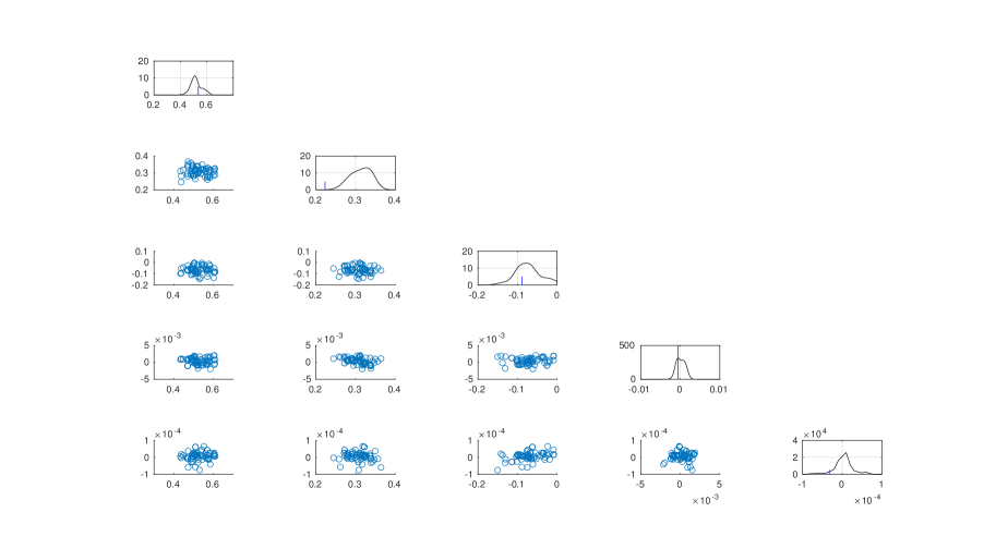
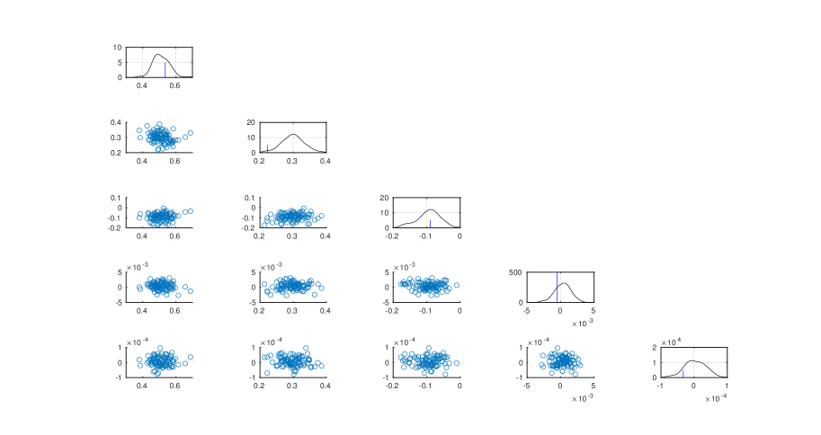
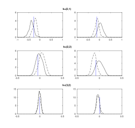
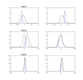
When tempering is used we present in Figure 1 selected typical estimated PDFs and scatter plots for a few chosen frequencies -s. In the scatter plots the advantage of using (13) (in the bottom plot of Figure 1) results in higher dispersion of the particles relative to sampling from (6) (top plot). This is also apparent in the tails of the estimated PDFs. In Table 1 it is evident that when using tempering, IS resulted in about half of the tempering steps than when sampling from (6). In both cases, the tuning of the MCMC steps lead to the same acceptance ratio (around at the final tempering step). We use MCMC iterations per tempering for . For , plain tempering uses and IS with (13) uses . In addition, the IS-tempering case uses a larger step size (smaller ) for the MCMC (with rather than ). This results in lower total computational cost and runtimes when IS is used despite the added computations imposed by computing in (13). We also note that a lower number of tempering steps is beneficial in addressing potential path degeneracy issues. In Table 2 we present results when and to illustrate the robustness of Algorithm 2 w.r.t spacing of observation times and signal to noise ratio. As expected more tempering steps are needed in the more informative observation case (), but at the same time accurate observations result in lower errors. In addition, our method seems to perform comparatively better when . This can be attributed to the guided proposal being given more time to evolve and guide the particles to better regions of the state space.
| Tempering steps | ||||||||||||
|---|---|---|---|---|---|---|---|---|---|---|---|---|
|
5.6 | 4.7 | 4.4 | 4 | 4.3 | 64.87 | 73.88 | 63.02 | 57.01 | 53.03 | ||
|
5.9 | 4.3 | 4.0 | 4.0 | 4.1 | 54.16 | 53.79 | 40.29 | 90.06 | 54.53 | ||
|
5.1 | 4.6 | 4.6 | 4.6 | 5.1 | 65.25 | 45.23 | 80.27 | 99.78 | 82.45 | ||
|
4.6 | 3.7 | 3.2 | 3.1 | 3.9 | 39.97 | 88.61 | 48.99 | 49.21 | 80.08 | ||
|
7.2 | 6.0 | 5.9 | 5.7 | 6.1 | 65.27 | 74.57 | 51.94 | 54.57 | 50.26 | ||
| -errors | |||||||
|---|---|---|---|---|---|---|---|
|
|||||||
|
|||||||
|
|||||||
|
|||||||
|
|||||||
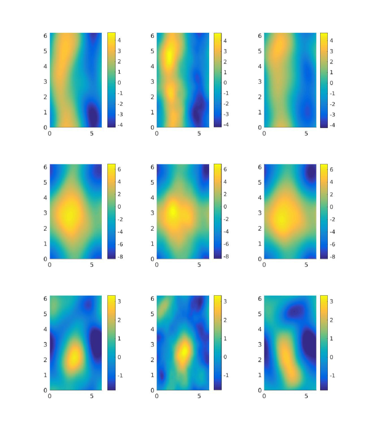
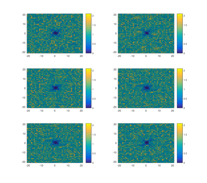
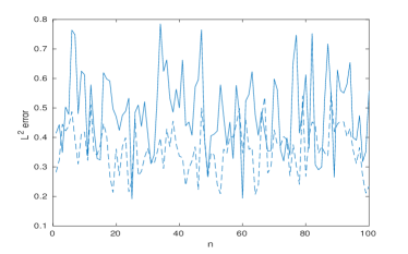
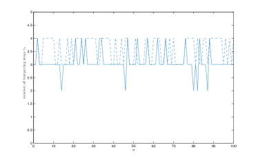
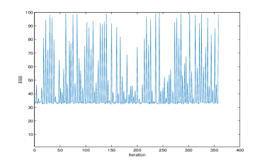
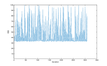
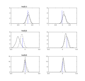
We proceed with the second numerical experiment, where we use only a single run of a PF with both tempering and IS for and . The dynamics for the state and true signal are as before, but for the observations we use a equally spaced observation grid and look at two different generated data-sets with different distributions for the noise : a zero mean Gaussian and zero mean Student-t distribution with 4 degrees of freedom. In both cases . For each case, different PFs are implemented, each with the correctly specified likelihood. In Figure 2 we plot the estimated vorticity posterior mean for , in each case together with the vorticity of the true signal. The estimates seem accurate with small deviations between the posterior mean and the true signal. The latter is sensible given the coarseness of the grid and the moderate number of observations. We also provide in Figure 3 a plot of the ratio of the posterior variance of the vorticity of over the unconditional variance when obeying the probability law determined by the stochastic NSE dynamics in (6). The information gain appears as a reduction in the posterior variance for low relative to the prior, which is to be expected as the spatial grid cannot be informative for higher wave-numbers. In Figure 4 we plot , -errors as before and number of tempering steps per iteration. In both cases the performance is fairly stable with time and the algorithm provides good posterior mean estimates. For completeness, in Figure 5 we include a comparison with the EnKF in terms of errors. The PF with IS and tempering performs much better. Finally, in Figure 6 we present some estimated PDFs. These plots capture for different . Notice that the true parameter (displayed as a vertical line) lies in regions where the mass of the estimated posterior density is high and the posterior variance for the t-distributed case is higher for low .

6 Discussion
We have presented a particle filtering methodology that uses likelihood-informed IS proposals, tempering and MCMC moves for signals obeying the stochastic NSE observed with additive noise. The approach is computationally intensive and requires a significant number of particles , but we believe the cost is quite moderate relatively to the dimensionality of the problem. The use of tempering and MCMC steps is crucial for this high-dimensional application. The inclusion of likelihood-informed proposals results in higher efficiency and , less tempering steps and higher step sizes for the MCMC steps - thus, overall, in lower computational cost. The IS proposals were designed using a Gaussian noise assumption for the observations, but we demonstrated numerically that they are still useful and efficient for observation noise obeying a Student-t distribution with heavier tails. In addition, as increases using proposals as in (13) will be more beneficial.
In the experiments presented in Section 5 the effective dimensionality of the problem is determined by and More challenging parameterizations than the ones presented here could be dealt with by increasing or via a more advanced numerical method for the solution of the SPDE. These can be addressed using the extensions discussed in Section 4.3.1. Another potentially useful extension is to use different number of particles for different ranges of following [28]. Furthermore we note that we did not make use of parallelization, but this is certainly possible for many parts of Algorithm 2 and can bring significant execution speed-ups in applications.
Future work could aim to extend this methodology by designing suitable IS proposals for non-linear observation schemes or observations obtained from Lagrangian drifters or floaters. Finally, an interesting question is whether an error analysis along the lines of [12, Section 7.4] can be reproduced. The simulations presented here seem to indicate roughly constant errors with time, but a rigorous treatment would need to establish the stability properties of the filtering distribution w.r.t the initialization.
Acknowledgements
FPLl was supported by EPSRC and the CDT in the Mathematics of Planet Earth under grant EP/L016613/1. AJ was supported by an AcRF tier 2 grant: R-155-000-161-112. AJ is affiliated with the Risk Management Institute, the Center for Quantitative Finance and the OR & Analytics cluster at NUS. AB was supported by the Leverhulme Trust Prize.
Appendix A More simulation results
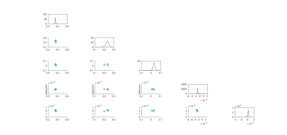
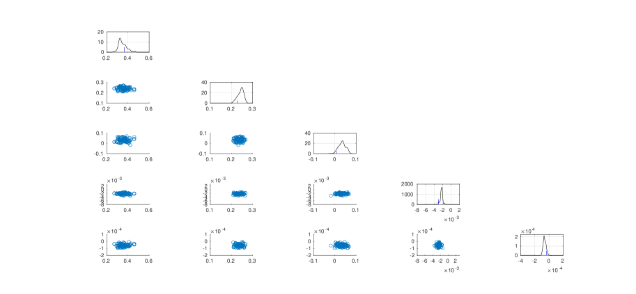
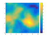
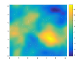
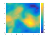
We present some negative numerical results to illustrate that tempering is necessary. We will consider a perfect initialization for each particle with . Whilst this is an extremely favorable scenario that is unrealistic in practice, it shows a clear benefit in using IS and tempering. For , and , we present some scatter plots in Figure 7 for the experiment with seen earlier with a block of observations. Notably, the estimated posterior means for the vorticity seem to exhibit good performance; see Figure 8. Indicatively, the ESS here is for IS and for the bootstrap case. Even in this extremely favorable scenario, the ESS is low and this strongly motivates the use of tempering to improve the efficiency of the particle methodology. In results not shown here, we also experimented the size of time increment a naive particle filter (Algorithm 1) can handle with perfect initialization. When the likelihood-informed proposals in (13) are used, the method produces accurate point estimates for up to . This is in contrast to when sampling from the dynamics, where the bootstrap version of Algorithm 1 can handle only up to .
References
- [1] A. Bain and D. Crisan, Fundamentals of stochastic filtering, Springer, 2008.
- [2] A. F. Bennett, Inverse modeling of the ocean and atmosphere, Cambridge University Press, 2005.
- [3] A. Beskos, D. Crisan, A. Jasra, K. Kamatani, and Y. Zhou, A stable particle filter for a class of high-dimensional state-space models, Advances in Applied Probability, 49 (2017), pp. 24–48.
- [4] A. Beskos, A. Jasra, N. Kantas, and A. Thiery, On the convergence of adaptive sequential Monte Carlo methods, The Annals of Applied Probability, 26 (2016), pp. 1111–1146.
- [5] M. Bocquet, C. A. Pires, and L. Wu, Beyond Gaussian statistical modeling in geophysical data assimilation, Monthly Weather Review, 138 (2010), pp. 2997–3023.
- [6] N. Chopin, A sequential particle filter method for static models, Biometrika, 89 (2002), pp. 539–552.
- [7] A. J. Chorin and P. Krause, Dimensional reduction for a Bayesian filter, Proceedings of the National Academy of Sciences of the United States of America, 101 (2004), pp. 15013–15017.
- [8] A. J. Chorin, M. Morzfeld, and X. Tu, Implicit particle filters for data assimilation, Communications in Applied Mathematics and Computational Science, 5 (2010), pp. 221–240.
- [9] S. L. Cotter, G. O. Roberts, A. M. Stuart, and D. White, MCMC methods for functions: modifying old algorithms to make them faster, Statistical Science, 28 (2013), pp. 424–446.
- [10] T. Cui, K. J. Law, and Y. M. Marzouk, Dimension-independent likelihood-informed MCMC, Journal of Computational Physics, 304 (2016), pp. 109–137.
- [11] G. Da Prato and J. Zabczyk, Stochastic equations in infinite dimensions, Cambridge University Press, 2008.
- [12] P. Del Moral, Feynman-Kac Formulae, Springer, 2004.
- [13] P. Del Moral, Mean field simulation for Monte Carlo integration, CRC Press, 2013.
- [14] P. Del Moral, A. Doucet, and A. Jasra, Sequential Monte Carlo samplers, Journal of the Royal Statistical Society: Series B (Statistical Methodology), 68 (2006), pp. 411–436.
- [15] A. Doucet, M. Briers, and S. Sénécal, Efficient block sampling strategies for sequential Monte Carlo methods, Journal of Computational and Graphical Statistics, 15 (2006), pp. 693–711.
- [16] A. Doucet, N. de Freitas, and N. Gordon, Sequential Monte Carlo methods in practice, Springer Science & Business Media, 2001.
- [17] G. Evensen, Data assimilation: the ensemble Kalman filter, Springer, 2009.
- [18] B. Ferrario, Stochastic Navier-Stokes equations: Analysis of the noise to have a unique invariant measure, Annali di Matematica Pura ed Applicata, 177 (1999), pp. 331–347.
- [19] F. Flandoli, Dissipativity and invariant measures for stochastic Navier-Stokes equations, Nonlinear Differential Equations and Applications NoDEA, 1 (1994), pp. 403–423.
- [20] F. Giraud and P. Del Moral, Nonasymptotic analysis of adaptive and annealed Feynman–Kac particle models, Bernoulli, 23 (2017), pp. 670–709.
- [21] S. Godsill and T. Clapp, Improvement strategies for Monte Carlo particle filters, [16], pp. 139–158.
- [22] A. Golightly and D. J. Wilkinson, Bayesian inference for nonlinear multivariate diffusion models observed with error, Computational Statistics & Data Analysis, 52 (2008), pp. 1674–1693.
- [23] V. H. Hoang, K. J. Law, and A. M. Stuart, Determining white noise forcing from Eulerian observations in the Navier-Stokes equation, Stochastic Partial Differential Equations: Analysis and Computations, 2 (2014), pp. 233–261.
- [24] M. Jardak, I. Navon, and M. Zupanski, Comparison of sequential data assimilation methods for the Kuramoto–Sivashinsky equation, International journal for numerical methods in fluids, 62 (2010), pp. 374–402.
- [25] A. Jasra, D. A. Stephens, A. Doucet, and T. Tsagaris, Inference for Lévy-driven stochastic volatility models via adaptive sequential Monte Carlo, Scandinavian Journal of Statistics, 38 (2011), pp. 1–22.
- [26] A. Jentzen and P. E. Kloeden, Overcoming the order barrier in the numerical approximation of stochastic partial differential equations with additive space–time noise, in Proceedings of the Royal Society of London A: Mathematical, Physical and Engineering Sciences, vol. 465, 2009, pp. 649–667.
- [27] A. M. Johansen, On block, tempering and particle mcmc for systems identification, in Proceedings of 17th IFAC Symposium on System Identification, IFAC, 1998.
- [28] A. M. Johansen, N. Whiteley, and A. Doucet, Exact approximation of Rao–Blackwellised particle filters, IFAC Proceedings Volumes, 45 (2012), pp. 488–493.
- [29] N. Kantas, A. Beskos, and A. Jasra, Sequential Monte Carlo methods for high-dimensional inverse problems: A case study for the Navier–Stokes equations, SIAM/ASA Journal on Uncertainty Quantification, 2 (2014), pp. 464–489.
- [30] S. Kuksin and A. Shirikyan, Mathematics of two-dimensional turbulence, vol. 194, Cambridge University Press, 2012.
- [31] K. Law, A. Stuart, and K. Zygalakis, Data assimilation: a mathematical introduction, vol. 62, Springer, 2015.
- [32] K. J. Law, Proposals which speed up function-space MCMC, Journal of Computational and Applied Mathematics, 262 (2014), pp. 127–138.
- [33] A. Lee, C. Yau, M. B. Giles, A. Doucet, and C. C. Holmes, On the utility of graphics cards to perform massively parallel simulation of advanced Monte Carlo methods, Journal of Computational and Graphical Statistics, 19 (2010), pp. 769–789.
- [34] A. J. Majda and J. Harlim, Filtering complex turbulent systems, Cambridge University Press, 2012.
- [35] R. M. Neal, Annealed importance sampling, Statistics and Computing, 11 (2001), pp. 125–139.
- [36] N. Papadakis, É. Mémin, A. Cuzol, and N. Gengembre, Data assimilation with the weighted ensemble Kalman filter, Tellus A, 62 (2010), pp. 673–697.
- [37] O. Papaspiliopoulos and G. Roberts, Importance sampling techniques for estimation of diffusion models, Statistical methods for stochastic differential equations, 124 (2012), pp. 311–340.
- [38] O. Papaspiliopoulos, G. O. Roberts, and O. Stramer, Data augmentation for diffusions, Journal of Computational and Graphical Statistics, 22 (2013), pp. 665–688.
- [39] S. Särkkä and E. Moulines, On the Lp-convergence of a Girsanov theorem based particle filter, in Acoustics, Speech and Signal Processing (ICASSP), 2016 IEEE International Conference on, IEEE, 2016, pp. 3989–3993.
- [40] S. Särkkä, T. Sottinen, et al., Application of Girsanov theorem to particle filtering of discretely observed continuous-time non-linear systems, Bayesian Analysis, 3 (2008), pp. 555–584.
- [41] C. Snyder, T. Bengtsson, P. Bickel, and J. Anderson, Obstacles to high-dimensional particle filtering, Monthly Weather Review, 136 (2008), pp. 4629–4640.
- [42] A. M. Stuart, Inverse problems: a Bayesian perspective, Acta Numerica, 19 (2010), pp. 451–559.
- [43] L. Tierney, A note on Metropolis-Hastings kernels for general state spaces, Annals of Applied Probability, (1998), pp. 1–9.
- [44] F. van der Meulen and M. Schauer, Bayesian estimation of incompletely observed diffusions, arXiv preprint arXiv:1606.04082, (2016).
- [45] P. J. van Leeuwen, Nonlinear data assimilation in geosciences: an extremely efficient particle filter, Quarterly Journal of the Royal Meteorological Society, 136 (2010), pp. 1991–1999.
- [46] P. J. Van Leeuwen, Y. Cheng, and S. Reich, Nonlinear Data Assimilation, Springer, 2015.
- [47] J. Weare, Particle filtering with path sampling and an application to a bimodal ocean current model, Journal of Computational Physics, 228 (2009), pp. 4312–4331.
- [48] G. A. Whitaker, A. Golightly, R. J. Boys, and C. Sherlock, Improved bridge constructs for stochastic differential equations, Statistics and Computing, (2016), pp. 1–16.