Grid peeling and the affine curve-shortening flow

Abstract

In this paper we study an experimentally-observed connection between two seemingly unrelated processes, one from computational geometry and the other from differential geometry. The first one (which we call grid peeling) is the convex-layer decomposition of subsets $G\subset\mathbb{Z}^{2}$ of the integer grid, previously studied for the particular case $G=\{1,\ldots,m\}^{2}$ by Har-Peled and Lidický (2013). The second one is the affine curve-shortening flow (ACSF), first studied by Alvarez et al. (1993) and Sapiro and Tannenbaum (1993). We present empirical evidence that, in a certain well-defined sense, grid peeling behaves at the limit like ACSF on convex curves. We offer some theoretical arguments in favor of this conjecture.

We also pay closer attention to the simple case where $G=\mathbb{N}^{2}$ is a quarter-infinite grid. This case corresponds to ACSF starting with an infinite L-shaped curve, which when transformed using the ACSF becomes a hyperbola for all times $t>0$. We prove that, in the grid peeling of $\mathbb{N}^{2}$, (1) the number of grid points removed up to iteration $n$ is $\Theta(n^{3/2}\log n)$; and (2) the boundary at iteration $n$ is sandwiched between two hyperbolas that are separated from each other by a constant factor.

1 Introduction

Let $G$ be a planar point set. The convex-layer decomposition (or onion decomposition) of $G$ [6, 8, 12, 14, 16] is a discrete algorithmic process in which points of $G$ are iteratively removed, as follows: Let $G_{0}=G$. Then, for each $n\geq 1$ such that $G_{n-1}\neq\emptyset$, let $H_{n}=\operatorname{\mathcal{CH}}{(G_{n-1})}$ (the convex hull of the current set), let $L_{n}$ be the set of vertices of $H_{n}$, and remove $L_{n}$ from the current set by setting $G_{n}=G_{n-1}\setminus L_{n}$. We call $H_{n}$ the $n$th convex layer of $G$. This decomposition has applications in range-searching data structures [9] and as a measure of depth in robust statistics [6, 14].

Motivated by the question of whether grid points behave similarly to random points, Har-Peled and Lidický [16] studied the convex-layer decomposition of the $m\times m$ integer grid $G=\{1,\ldots,m\}^{2}$. They proved that this point set has $\Theta(m^{4/3})$ convex layers. They also briefly noted that the convex layers of this point set appear to converge to circles as the process advances.

In this paper we explore an experimentally-observed connection between the convex-layer decomposition of more general subsets $G\subset\mathbb{Z}^{2}$ of the integer grid (which we call grid peeling), and a continuous process on smooth curves known as the affine curve-shortening flow (ACSF). Our conjectural connection between these two processes, if true, would show that in the square case studied by Har-Peled and Lidický, peeling indeed converges to a circular shape. More generally, it would show that for any convex shape, in the limit as the grid density becomes arbitrarily fine, the result of peeling the intersection of that shape with a grid converges to an ellipse.

1.1 The affine curve-shortening flow

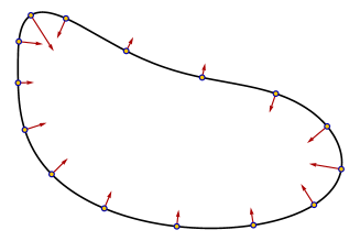
In the affine curve-shortening flow, a smooth curve $\gamma\subset\mathbb{R}^{2}$ varies with time in the following way. At each moment in time, each point of $\gamma$ moves perpendicularly to the curve, towards its local center of curvature, with instantaneous velocity $r^{-1/3}$, where $r$ is that point’s radius of curvature at that time. Thus, for a smooth convex curve, all points move inwards, possibly at different velocities. For non-convex curves, points of local non-convexity move outwards. See Figure 1.

Figure 1: Affine curve-shortening flow. The arrows indicate the instantaneous velocity of different points along the curve at the shown time moment.

The ACSF was first studied by Alvarez et al. [1] and Sapiro and Tannenbaum [24]. It differs from the more usual curve-shortening flow (CSF) [7, 11], in which each point moves with instantaneous velocity $r^{-1}$. Unlike the CSF, the ACSF is invariant under affine transformations: Applying an affine transformation to a curve, and then performing the ACSF, gives the same results (after rescaling the time parameter appropriately) as performing the ACSF and then applying the affine transformation to the shortened curves. Moreover, if the affine transformation preserves area, then the time scale is unaffected. For more on the ACSF see [7, 10, 18] and references cited there.

For the CSF, every smooth Jordan curve eventually becomes convex and then converges to a circle as it collapses to a point, without ever crossing itself. Angenent et al. [3] proved that, correspondingly, under the ACSF, every smooth Jordan curve becomes convex and then converges to an ellipse as it collapses to a point, without self-crossings.

Even if the initial curve $\gamma$ is not smooth (e.g. it has sharp corners), as long as it satisfies certain natural conditions, there exists a unique time-dependent curve $\gamma(t)$ which satisfies the ACSF (or the CSF) condition for all $t>0$, and which converges to $\gamma$ as $t\to 0^{+}$. See [7], Theorems 3.26 and 3.28.

The ACSF was originally applied in computer vision, as a way of smoothing object boundaries [7] and of computing shape descriptors that are insensitive to the distortions caused by changes of viewpoint. Because peeling can be computed quickly and efficiently, by a purely combinatorial algorithm [8], our conjectural connection between peeling and the ACSF could potentially provide an efficient way of performing these computations. However, to fully realize this potential application, it would be helpful to prove rigorous bounds on the accuracy of approximation, and to find a way to generalize the approximation so that it can handle non-convex curves as well. In the other direction, our conjecture would allow us to apply results on the well-understood behavior of the ACSF to the less well-understood algorithmic process of grid peeling. For instance, it would explain the circular layer shapes observed by Har-Peled and Lidický.

1.2 Organization of this paper

This paper is organized as follows. In Section 2 we formalize our conjectured connection between peeling and the ACSF as Section 2, and provide a non-rigorous justification for the conjecture. In Section 3 we describe our implementation details, and report on more detailed experiments that quantify the similarity between peeling and the ACSF. In Section 4 we prove Theorem 1, which shows that for bounded regions, the rates of peeling and the ACSF are within a constant factor of each other, a weaker form of our conjecture. In Section 5 we examine more closely a special case of our conjecture on a quarter-infinite grid, and prove more precise results for that case.

2 The connection

Empirical evidence points to a connection between grid peeling and the ACSF. For a curve $\gamma$, let $\gamma(t)$, $t\geq 0$, be the result of applying ACSF on $\gamma$ for time duration $t$. Given a positive integer $n$, let $(\mathbb{Z}/n)^{2}$ be the uniform grid with spacing $1/n$. Given a convex region $R\subset\mathbb{R}^{2}$, let $G_{[n]}(R)=R\cap(\mathbb{Z}/n)^{2}$ be the set of grid points of $(\mathbb{Z}/n)^{2}$ contained in $R$. Informally, for a convex curve $\gamma$, we have that peeling $G_{[n]}(\operatorname{\mathcal{CH}}(\gamma))$ appears to approximate the ACSF on $\gamma$ as $n\to\infty$.

This connection is illustrated in Figure 2. Figure 2 (left) shows the ACSF evolution of a sample convex curve $\gamma$, given by $\gamma=\{(x(a),y(a)):0\leq a<2\pi\}$ for $x(a)=((1-\sin{a})/2)^{2}$ and $y(a)=((1-\sin{(a+2)})/2)^{1.3}$. Specifically, the figure shows $\gamma(0.02t)$ for $t=0,1,2,\ldots,14$. Figure 2 (center) shows every fifth layer of the convex-layer decomposition of $G_{[30]}(R)$ for $R=\operatorname{\mathcal{CH}}(\gamma)$. The similarity to Figure 2 (left) is immediately evident. Finally, Figure 2 (right) shows every $2714$th layer of the convex-layer decomposition of $G_{[5000]}(R)$. Figure 2 (left) and (right) are virtually indistinguishable to the naked eye.

Figure 2: Left: ACSF evolution of a convex curve. Center and right: Convex-layer decomposition of the set of grid points inside the same convex curve, for different grid spacings.

We can formalize this resemblance by the following conjecture.

Conjecture .

There exists a constant $c\approx 1.6$ such that the following is true: Let $R\subset\mathbb{R}^{2}$ be a convex region, and let $\gamma=\partial R$ be its boundary. Let $t^{*}$ be the time it takes for $\gamma$ to collapse to a point under the ACSF (or $t^{*}=\infty$ for unbounded sets that never collapse). Fix a time $0\leq t<t^{*}$, and let $\gamma^{\prime}=\gamma(t)$ under the ACSF. For a fixed $n$, let $G^{\prime}$ be the $m$th convex layer of $G_{[n]}(R)$ for

$$m=ctn^{4/3}.$$ (1)

Then, as $n\to\infty$, the boundary of the convex hull of $G^{\prime}$ converges pointwise to $\gamma^{\prime}$.

In particular, the ACSF is known to converge to an ellipse for any closed initial boundary $\gamma$, in the limit as $t\to t^{*}$, when its shape is rescaled to have constant area. Correspondingly, by the conjecture, the convex layers of $G_{[n]}(R)$ should also converge to ellipses as $t\to t^{*}$ and $n\to\infty$. By symmetry, the convex layers of a square grid should indeed converge to circles.

2.1 Justification for Section 2

One intuitive but somewhat vague justification for Section 2 is that the ACSF is invariant under affine transformations (in fact, it is the unique affine-invariant flow of least order [7]), and grid peeling is also invariant under a subgroup of affine transformations, namely the ones that preserve the unit grid.

A more detailed justification is as follows. Balog and Bárány [5] proved that, if $R$ is the unit disk, then $\operatorname{\mathcal{CH}}(G_{[n]}(R))$ has $\Theta(n^{2/3})$ vertices. Equivalently, if $R$ is a disk of radius $r$, then $C=\operatorname{\mathcal{CH}}(G_{[n]}(R))$ has $\Theta((nr)^{2/3})$ vertices. Let us assume these vertices are uniformly distributed along the boundary of $C$, so a portion of $\partial C$ of length $d$ contains $\Theta(dn^{2/3}r^{-1/3})$ vertices.

Now, let $R\subset\mathbb{R}^{2}$ be an arbitrary convex region with smooth boundary $\gamma=\partial R$, and fix a small portion $\delta$ of $\gamma$, of almost constant radius of curvature $r$. Let $d$ be the length of $\delta$. Let $C=\operatorname{\mathcal{CH}}(G_{[n]}(R))$ for large $n$. Then the portion $\delta^{\prime}$ of $\partial C$ that is close to $\delta$ contains $\Theta(dn^{2/3}r^{-1/3})$ vertices. Let $\varepsilon>0$ be much smaller than $d$. In order for $\delta^{\prime}$ to advance inwards by distance $\varepsilon$, a total of $\varepsilon dn^{2}$ grid points must be removed. This should take $\Theta(\varepsilon n^{4/3}r^{1/3})$ iterations. Therefore, $\delta^{\prime}$ should move inwards at speed $\Theta(n^{-4/3}r^{-1/3})$. This is $\Theta(n^{4/3})$ times slower than ACSF, independently of $r$.

3 Implementation and experiments

We first implemented a simple front-tracking ACSF approximation method that works as follows. We sample a number $m$ of points $p_{1},\ldots,p_{m}$ along the given curve $\gamma$. For each point $p_{i}$, we estimate the normal vector and the radius of curvature at $p_{i}$ by the normal vector $v_{i}$ and radius $r_{i}$ of the unique circle passing through points $p_{i-1},p_{i},p_{i+1}$. We simultaneously let all points move at the appropriate speeds for a short time interval $t=c\cdot(d_{\mathrm{min}})^{4/3}$, where $d_{\mathrm{min}}$ is the minimum distance between two consecutive points, and $c$ is a fixed parameter. Then we repeat the process. Hence, as the sample points get closer and closer, we take smaller and smaller time steps. Here the exponent $4/3$ was chosen in order for the simulation to be scale-independent.

A disadvantage of this method is that, as the curve becomes elliptical, the sample points tend to bunch together at the sharp ends of the ellipse, causing the time step to decrease very drastically. In order to overcome this problem, we then implemented a more sophisticated approach, in which each point is also given a tangential velocity component $w_{i}$ (i.e. $w_{i}\perp v_{i}$). (Tangential velocities should not affect the evolution of a flow, since they only cause curve points to move within the curve.) We make the length of $w_{i}$ proportional to $\|v_{i}\|\cdot\log(\|p_{i}-p_{i-1}\|/\|p_{i}-p_{i+1}\|)$. Hence, if $p_{i}$ is equidistant from $p_{i-1}$ and $p_{i+1}$, then $\|w_{i}\|=0$. Otherwise, if $p_{i}$ is closer to $p_{i-1}$ than to $p_{i+1}$, say, then $w_{i}$ points in the direction of $p_{i+1}$.

This simple approach was enough for our purposes. For more advanced flow simulation methods, see e.g. [7, 15, 21] and references cited there.

Our ACSF C++ program may be found at ACSF.cpp, in the ancillary files of this paper.

For the grid peeling simulations, we represent the grid subset as a one-dimensional array that stores, for each row, the $x$-coordinates of the leftmost and rightmost grid points in that row. We compute the convex hull at each iteration using Andrew’s modification of Graham’s scan [2, 13]. Thus, to find the $\Theta(n^{4/3})$ layers of an $n\times n$ grid we take $O(n)$ time per layer and $O(n^{7/3})$ time overall. Faster $O(n^{2}\log n)$-time algorithms are possible [8, 22, 23] but were unnecessary for our experiments. We implemented this peeling algorithm in two C++ programs, “peel N2.cpp” (for peeling $\mathbb{N}^{2}$) and “peel shape.cpp” (for peeling general shapes).

3.1 Experiments on bounded regions

In order to test Section 2, we ran both ACSF and grid peeling on several bounded convex regions, and compared the results. The regions we used are: $R_{1}=\operatorname{\mathcal{CH}}(\gamma)$ for the curve $\gamma$ of Figure 2; $R_{2}$, a square of side $1$; $R_{3}$, a triangle with vertices $(0,0)$, $(1,3/4)$, $(2/5,1)$; $R_{4}$, a half-disk of diameter $1$; and $R_{5}$, a disk of diameter $1$.

Figure 3: Comparison between ACSF (left) and grid peeling (right) on several test shapes.

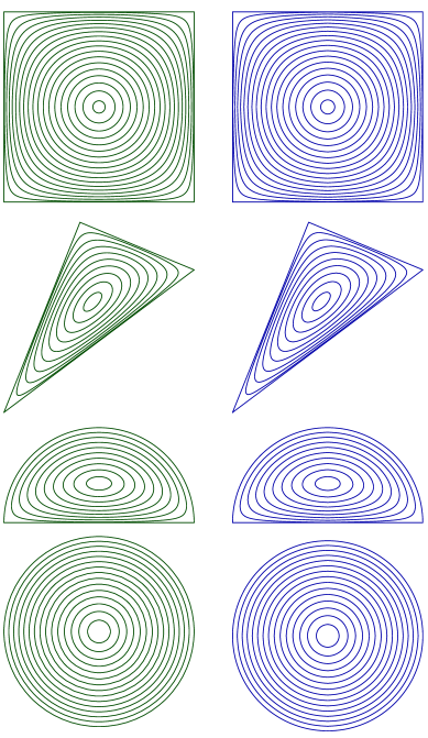
Figure 3 shows the results for $R_{2},\ldots,R_{5}$. Just as in Figure 2, here each left figure shows ACSF with time steps of $0.02$, and each right figure shows every $2714$th convex layer, starting with a grid of spacing $1/5000$. Each left figure is barely distinguishable to the naked eye from the corresponding right figure.

In order to further test Section 2, we took the same regions $R_{1},\ldots,R_{5}$, and measured the Hausdorff distance between the results of the two processes, for increasing values of the grid density $n$. For each $R_{i}$, we first ran our ACSF simulation with higher-precision parameters, until the times $t_{1},\ldots,t_{5}$ at which the area enclosed by the curve decreased to $95\%,90\%,\ldots,75\%$ of its original area. Then we ran grid peeling using a variety of grid spacings; specifically, $1/n$ for $n=1000,3000,10000,30000,100000$. In each case, we ran the process until the times $m_{1},\ldots,m_{5}$ at which the number of grid points decreased to $95\%,\ldots,75\%$ of its original value.

For each case, we then computed the Hausdorff distance between the ACSF curve and the grid-peeling curve, both represented as polygonal chains. (For comparison, we also computed the initial Hausdorff distance, which reflects the inherent inaccuracy in approximating the given smooth curve by grid points.) Figure 4 shows the results.

Figure 4: Hausdorff distance between the results of ACSF and grid peeling, for a variety of test shapes, times, and grid spacings.

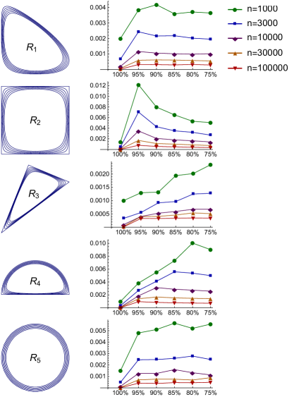
As we can see, the Hausdorff distance decreases with increasing $n$. Furthermore, for large values of $n$, the length of time has no major effect on the Hausdorff distance.

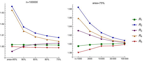
Finally, we checked whether the ACSF times $t_{1},\ldots,t_{5}$ are related to the grid peeling times $m_{1},\ldots,m_{5}$ in the manner predicted by Section 2. To do this, we solved for the constant $c$ in (1), and computed the approximations $c\approx m_{i}/(t_{i}n^{4/3})$. The results are shown in Figure 5. As can be seen, in all cases we obtained values close to $1.6$; furthermore, the approximations get closer to each other as either $n$ or $t$ increases.

Figure 5: Approximations of the constant $c$ given by the experiments. The left plot uses the data for $n=100000$ and various values of the final area. The right plot uses the data for a final area of $75\%$ and various values of $n$.

4 Number of convex layers for bounded regions

In this section we prove that for bounded regions $R$, Section 2 is asymptotically correct as far as the number of convex layers is concerned:

Theorem 1.

Let $R\subset\mathbb{R}^{2}$ be a bounded convex region. Then the number of convex layers of $G_{[n]}(R)$ is $\Theta(n^{4/3})$, with a constant of proportionality that depends on $R$.

Correspondingly, in ACSF, if the given curve $\gamma$ is dilated by a factor of $k$, then its evolution is dilated in time by a factor of $k^{4/3}$.

Theorem 1 follows from the result of [16] on the number of convex layers of square grids. First, we note that the result of [16] can be readily generalized to rectangular grids using the same argument:

Lemma .

Let $m,n$ be integers satisfying $\sqrt{m}\leq n\leq m^{2}$. Then the number of convex layers of $G=\{1,\ldots,m\}\times\{1,\ldots,n\}$ is $\Theta\bigl{(}m^{2/3}n^{2/3}\bigr{)}$.

Now, let $R\subset\mathbb{R}^{2}$ be a given bounded convex region. By John’s ellipsoid theorem [20], there exist two ellipses that satisfy $E_{1}\subseteq R\subseteq E_{2}$, such that the ratio between their areas is at most $4$.

Let $n$ be an integer, and let $G=G_{[n]}(R)$. Scale up all these sets by a factor of $n$, obtaining $R^{\prime}$, $E^{\prime}_{1}$, $E^{\prime}_{2}$, and $G^{\prime}\subset\mathbb{Z}^{2}$. The grid peeling process is clearly invariant to linear transformations. We now focus on grid-preserving linear transformations, that is, linear transformations that map $\mathbb{Z}^{2}$ bijectively into $\mathbb{Z}^{2}$. A linear transformation $f:\mathbb{R}^{2}\to\mathbb{R}^{2}$ is grid-preserving if and only if it is of the form $f(p)=Mp$, where $M$ is a $2\times 2$ integer matrix with determinant $\pm 1$.

Lemma .

Let $v_{1},v_{2}\in\mathbb{Z}^{2}$ be linearly independent vectors. Then there exists a grid-preserving linear transformation $f$ that maps $v_{1}$ into the $x$-axis, and such that $f(v_{2})$ has slope at least $2$ in absolute value.

Proof.

We first apply a grid-preserving linear transformation $f_{1}$ that maps $v_{1}$ to the $x$-axis. Denote $f_{1}(v_{2})=(x_{2},y_{2})$. Then we apply a horizontal shear $f_{2}:(x,y)\mapsto(x-my,y)$, for an appropriate $m\in\mathbb{Z}$. The appropriate $m$ is either $\lfloor y_{2}/x_{2}\rfloor$ or $\lceil y_{2}/x_{2}\rceil$. ∎

Now, the ellipse $E^{\prime}_{1}$ contains a rectangle $T_{1}$ whose area is at least a constant fraction of the area of $E_{1}$. Applying Section 4, we turn $T_{1}$ into a parallelogram $T^{\prime}_{1}$ with two horizontal sides and two shorter, close-to-vertical sides. Hence, $T^{\prime}_{1}$ contains an axis-parallel rectangle $T^{\prime\prime}_{1}$ whose area is at least a constant fraction of the area of $T^{\prime}_{1}$. If $n$ is large enough, then the side lengths $m_{1}$ and $m_{2}$ of $T^{\prime\prime}_{1}$ will satisfy $\sqrt{m}_{1}\leq m_{2}\leq m_{1}^{2}$. Therefore, we can apply the lower bound of Section 4 on $T^{\prime\prime}_{1}$.

The upper bound proceeds similarly, using ellipse $E^{\prime}_{2}$. This completes the proof of Theorem 1.

5 Peeling a quarter-infinite grid

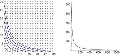
A simple test case for Section 2 is the region $R=\{(x,y):x\geq 0,y\geq 0\}$ (the first quadrant of the plane). In this case, the grid spacing $n$ is irrelevant, so we can simply take $G=\mathbb{N}^{2}$ (where $\mathbb{N}=\{0,1,2,\ldots\}$). The boundary of $R$ is the L-shaped curve $\gamma_{L}=\{(x,0):x\geq 0\}\cup\{(0,y):y\geq 0\}$.

The time-dependent hyperbola

$$\gamma_{L}(t)=\{(x,y):y=(4/3^{3/2})t^{3/2}/x\}.$$ (2)

satisfies the ACSF condition for all $t>0$ (as can be verified by a simple calculation), and it converges to $\gamma_{L}$ as $t\to 0^{+}$. The hyperbola (2) is the only solution satisfying this property.

Hence, by Section 2, we would expect the convex layers of $\mathbb{N}^{2}$ to approach hyperbolas as the process goes on. Indeed, this is what occurs experimentally. In the next subsections we present our experimental and theoretical results regarding the convex layers of $\mathbb{N}^{2}$. But let us first introduce some notation.

Figure 6: Left: Convex layers $5,10,15,\ldots,30$ of $\mathbb{N}^{2}$. Right: $1000$th convex layer of $\mathbb{N}^{2}$.

Notation.

Throughout this section, we will define the sets $G_{n},L_{n},H_{n}$ as in the Introduction for our choice of $G=\mathbb{N}^{2}$. Hence, $G_{0}=\mathbb{N}^{2}$, $H_{n}=\operatorname{\mathcal{CH}}{(G_{n-1})}$, $L_{n}$ is the set of vertices of $H_{n}$, and $G_{n}=G_{n-1}\setminus L_{n}$. Let $B_{n}=\partial H_{n}$. Let $(K_{n},K_{n})$ be the point of intersection of $B_{n}$ with the line $y=x$, so the point $(K_{n},K_{n})$ splits $B_{n}$ into two congruent “arms”. Let $s(n)=|L_{1}|+\cdots+|L_{n}|$ be the number of grid points removed up to iteration $n$. Given integers $x,n\in\mathbb{N}$, let $a_{x}(n)$ be the number of points of the $x$th column of $G$ that have been removed up to iteration $n$; i.e., let $a_{x}(n)=\bigl{|}\bigl{\{}(\{x\}\times\mathbb{N})\cap(L_{1}\cup\cdots\cup L_{n})\bigr{\}}\bigr{|}$. Note that in a fixed column, the points are removed in increasing order of $y$-coordinate; furthermore, for every fixed $n$ the sequence $a_{0}(n),a_{1}(n),a_{2}(n),\ldots$ is nonincreasing, with $a_{0}(n)=n$, $a_{n-1}(n)=1$, and $a_{n}(n)=0$. See Figure 6.

5.1 Experiments

Given $n$, let $B^{\prime}_{n}$ be the result of scaling down the $n$th layer boundary $B_{n}$ by a factor of $n^{3/4}$. According to Section 2, as $n\to\infty$ we would expect $B^{\prime}_{n}$ to converge to the hyperbola $\gamma_{L}(1/c)$ of (2). We would like to measure to what extent this happens. However, since we do not know the constant $c$ to high precision, we performed these measurements as follows:

Given $n$, let $f_{n}(x)=K_{n}^{2}/x$ define the hyperbola that passes through the point $(K_{n},K_{n})$. Given a small real number $0<\alpha<1$, let $x_{\alpha}(n)$ denote the smallest integer $x>K_{n}$ for which $|a_{x}(n)-f(x)|>\alpha f(x)$. Hence, the portion of $B_{n}$ that is between $x$-coordinates $x=K_{n}$ and $x=x_{\alpha}(n)$ is within an $\alpha$-fraction of the hyperbola $f(x)$. By symmetry, the same can be said about the portion of $B_{n}$ that is between $y$-coordinates $y=K_{n}$ and $y=x_{\alpha}(n)$. The ratio $x_{\alpha}(n)/K_{n}$ provides a scale-independent measure of the extent to which $B_{n}$ is $\alpha$-close to a hyperbola.

Figure 7: Measurements indicating that as $n$ increases, an increasingly long portion of $B_{n}$ is close to a hyperbola.

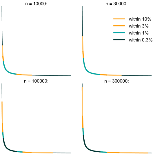
Figure 7 illustrates the results of these measurements for increasing values of $n$ and decreasing values of $\alpha$. Specifically, we took $n=10000,30000,100000,300000$ and $\alpha=0.1,0.03,0.01,0.003$. As can be seen, for each fixed $\alpha$, the portion of the hyperbola that is within an $\alpha$-fraction of $B_{n}$ grows as $n$ increases.

Figure 8: Approximations of the constant $c$ given by experimental measurements of the point $(K_{n},K_{n})$.

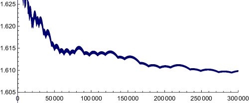
Measuring the time relationship.

Section 2 predicts that $K_{n}\approx 2(n/(3c))^{3/4}$ for large $n$. We tested this prediction by solving for $c$ and seeing whether it approaches a constant close to $1.6$. The results are shown in Figure 8.

Layer sizes.

The sequence $\{|L_{n}|\}$ represents the number of vertices in successive layers of the convex-layer decomposition of $\mathbb{N}^{2}$. This sequence is now cataloged in the Online Encyclopedia of Integer Sequences as A293596. It starts as

$$1,2,2,3,4,4,3,4,6,6,5,4,6,6,8,7,6,6,6,8,9,10,10,8,8,7,8,10,10,12,13,12,\ldots$$

Figure 9: Number of vertices of the $n$th convex layer of $\mathbb{N}^{2}$ as a function of $n$.

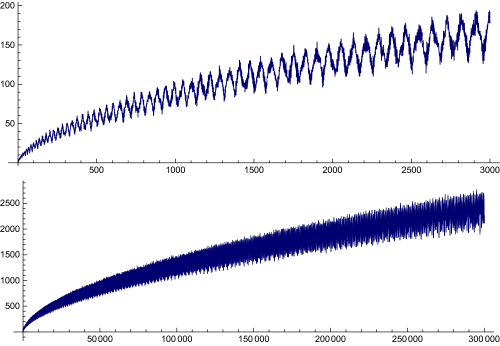
Figure 9 plots this sequence at different scales. As can be seen, this sequence has regular waves that slowly increase in both length and amplitude. Nevertheless, the relative amplitude of the waves (the ratio between their amplitude and their height above the $x$-axis) seems to decrease, perhaps tending to zero.

5.2 Rigorous results

We now obtain some rigorous results for the grid peeling of $G=\mathbb{N}^{2}$.

Figure 10: Schematic drawing of the upper and lower bounds for the $n$th convex layer of $\mathbb{N}^{2}$.

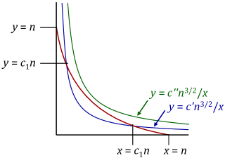
Theorem 2.

The convex-layer decomposition of the quarter-infinite grid $G=\mathbb{N}^{2}$ satisfies the following properties:

1. The number of grid points removed up to iteration $n$ satisfies $s(n)=\Theta(n^{3/2}\log n)$.

2. $a_{x}(n)=O(n^{3/2}/x)$ for all $n$, and $a_{x}(n)=\Omega(n^{3/2}/x)$ for $c_{1}\sqrt{n}\leq x\leq c_{1}n$, where $0<c_{1}<1$ is some constant.

3. $K_{n}=\Theta(n^{3/4})$.

4. $|L_{n}|=O(n^{1/2}\log n)$ and $|L_{n}|=\Omega(\log n)$.

In other words, the boundary $B_{n}$ is sandwiched between two hyperbolas that are separated from each other by a constant factor, where the upper hyperbola bounds $B_{n}$ for all $x$, while the lower hyperbola bounds $B_{n}$ only up to $x=c_{1}n$ (and symmetrically in the $y$-axis). Put differently, the scaled boundary $B^{\prime}_{n}$ is sandwiched between two hyperbolas $y\geq c_{1}x$ and $y\leq c_{2}x$ that are independent of $n$, where the lower hyperbola bounds $B^{\prime}_{n}$ only up to $x=c_{1}n^{1/4}$ (and symmetrically in the $y$-axis). See Figure 10.

Regarding $|L_{n}|$, we would expect it to behave like $\Theta(n^{1/2}\log n)$, or even like $c^{\prime}n^{1/2}\log n\pm o(n^{1/2}\log n)$ for some constant $c^{\prime}$. However, our rigorous lower bound for $|L_{n}|$ is very weak.

5.3 Proof of Theorem 2

The proof of Theorem 2 is mainly based on the techniques of [16].

Lemma (Jarník [19]).

Let $P\subset\{1,\ldots,m\}\times\{1,\ldots,n\}$ be in convex position. Then $|P|=O((mn)^{1/3})$.

Proof.

Let $p_{0},p_{1},p_{2}\ldots,p_{k-1}$ be the points of $P$ listed in circular order around the boundary of $\operatorname{\mathcal{CH}}{(P)}$, and let $v_{i}=p_{(i+1)\bmod k}-p_{i}$ be the vectors corresponding to the edges of $\operatorname{\mathcal{CH}}{(P)}$. Note that these vectors are pairwise distinct. Let $x_{\mathrm{max}}=m^{2/3}n^{-1/3}$ and $y_{\mathrm{max}}=n^{2/3}m^{-1/3}$. Classify the vectors $v_{i}=(x_{i},y_{i})$ into three types as follows: (1) Those satisfying $|x_{i}|\leq x_{\mathrm{max}}$ and $|y_{i}|\leq y_{\mathrm{max}}$; (2) those satisfying $|x_{i}|>x_{\mathrm{max}}$; (3) the remaining ones (which satisfy $|y_{i}|>y_{\mathrm{max}}$). The number of vectors of type (1) is at most $4x_{\mathrm{max}}y_{\mathrm{max}}=O((mn)^{1/3})$. The number of vectors of type (2) is at most $2m/x_{\mathrm{max}}=O((mn)^{1/3})$. And the number of vectors of type (3) is at most $2n/y_{\mathrm{max}}=O((mn)^{1/3})$. ∎

A vector $v=(x,y)\in\mathbb{Z}^{2}$ is said to be primitive if $x$ and $y$ are relatively prime.

Lemma .

Let $M=\{a+1,\ldots,a+m\}\times\{b+1,\ldots,b+n\}\subseteq\{1,\ldots,N\}^{2}$. Then the number of primitive vectors in $M$ is $(6/\pi^{2})mn\pm O(N\log N)$.

Proof.

We start with the following classical number-theoretical result.

Lemma .

Let $m,n$ be positive integers with $m\leq n$. Let $\rho(m,n)$ be the number of primitive vectors $(x,y)$ in $\{1,\ldots,m\}\times\{1,\ldots,n\}$. Then $\rho(m,n)=(6/\pi^{2})mn\pm O(n\log n)$.

Proof.

(Following Hardy and Wright [17], Theorem 332.) Let $\mu$ be the Möbius function, which sets $\mu(x)=-1$ if $x$ is square-free and has an odd number of prime factors, $\mu(x)=1$ if $x$ is square-free and has an even number of prime factors, and $\mu(x)=0$ if $x$ is not square-free. Let $D(x,y)$ be the set of all common divisors of $x$ and $y$. Then $\sum_{d\in D(x,y)}\mu(d)$ equals $1$ if $x$ and $y$ are relatively prime, and $0$ otherwise.

Clearly, $\sum_{x=1}^{\infty}\mu(x)/x^{2}$ converges to some positive real number smaller than $1$. In fact, it converges to $6/\pi^{2}$ [17].

Therefore,

$$\rho(m,n)=\sum_{x=1}^{m}\sum_{y=1}^{n}\sum_{d\in D(x,y)}\mu(d)=\sum_{d=1}^{mn}\mu(d)\left\lfloor\frac{m}{d}\right\rfloor\left\lfloor\frac{n}{d}\right\rfloor=\sum_{d=1}^{mn}\mu(d)\left(\frac{mn}{d^{2}}-O\left(\frac{n}{d}\right)\right)\\ =mn\sum_{d=1}^{mn}\frac{\mu(d)}{d^{2}}\pm O(n\log n)=mn\left(\sum_{d=1}^{\infty}\frac{\mu(d)}{d^{2}}\pm O\left(\frac{1}{mn}\right)\right)\pm O(n\log n),$$

and the claim follows. ∎

Now, consider $M=\{a+1,\ldots,a+m\}\times\{b+1,\ldots,b+n\}\subseteq\{1,\ldots,N\}^{2}$. The number of primitive vectors in $M$ equals $\rho(a+m,b+n)-\rho(a+m,b)-\rho(a,b+n)+\rho(a,b)$, so subsection 5.3 follows by subsection 5.3. ∎

5.3.1 Upper bounds

Lemma .

We have $a_{x}(n)\leq c_{0}n^{3/2}/x$ for some constant $c_{0}$.

Proof.

Given $x$, let $y=a_{x}(n)$. By iteration $n$, the entire corner subgrid $G^{\prime}=\{0,\ldots,x-1\}\times\{0,\ldots,y-1\}$ has been removed. By subsection 5.3, each $L_{i}$ contains $O((xy)^{1/3})$ points of $G^{\prime}$. Hence, we must have $xy\leq O(n(xy)^{1/3})$, which implies $y=O(n^{3/2}/x)$. ∎

Corollary .

We have $s(n)=O(n^{3/2}\log n)$.

Corollary .

We have $K_{n}\leq\sqrt{c_{0}}n^{3/4}$ for the constant $c_{0}$ of subsubsection 5.3.1.

Proof.

Take $x_{0}=\sqrt{c_{0}}n^{3/4}$, and note that $a_{x_{0}}(n)\leq x_{0}$. ∎

By subsubsection 5.3.1, each “arm” of $L_{n}$ is contained in an $O(n^{3/4})\times n$ box. Hence, a hasty application of subsection 5.3 would yield $|L_{n}|=O(n^{7/12})$. However, we can do better: We can cover each arm of $L_{n}$ by logarithmically many boxes of small area, and apply subsection 5.3 on each box.

Lemma .

We have $|L_{n}|=O(n^{1/2}\log n)$.

Proof.

Let $x_{0}=\sqrt{c_{0}}n^{3/4}$ for the constant $c_{0}$ of subsubsection 5.3.1, and recall that $K_{n}\leq x_{0}$. Define the axis-parallel boxes $T_{i}$, $0\leq i\leq\lceil\log_{2}(n/x_{0})\rceil$, by $T_{0}=[0,x_{0}]^{2}$ and $T_{i}=[2^{i-1}x_{0},2^{i}x_{0}]\times[0,x_{0}/2^{i}]$ for $i\geq 1$. By subsubsection 5.3.1, the right arm of $L_{n}$ is contained in the union of these boxes. Furthermore, the area of $T_{0}$ is $c_{0}n^{3/2}$, and the area of each $T_{i}$, $i\geq 1$, is $c_{0}n^{3/2}/2$. Hence, by subsection 5.3, each $T_{i}$ contains $O(\sqrt{n})$ points of $L_{n}$. Finally, the number of boxes is $O(\log n)$. ∎

5.3.2 Lower bounds

Figure 11: At the shown iteration, vector $v_{1}=(2,-3)$ is inactive, while vector $v_{2}=(2,-1)$ is active.

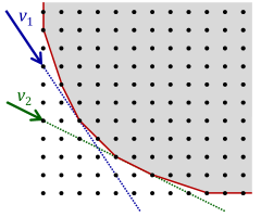
Let $v=(x_{v},-y_{v})$ be a primitive vector with $x_{v},y_{v}>0$. Following [16], we say that $v$ is active at iteration $n$ if the unique line $\ell_{v}$ parallel to $v$ that is tangent to $H_{n}$ contains an edge of $H_{n}$ (and so $\ell_{v}$ contains two points of $L_{n}$). Otherwise, if $\ell_{v}$ contains a single vertex of $H_{n}$ (and a single point of $L_{n}$), then we say that $v$ is inactive at iteration $n$. See Figure 11.

Given such a vector $v$, let $\mathcal{L}_{v}$ be the set of lines parallel to $v$ that pass through points of $\mathbb{N}^{2}$. We say that a line $\ell\in\mathcal{L}_{v}$ is alive at iteration $n$ if $\ell$ intersects $H_{n}$; otherwise, we say that $\ell$ is dead at iteration $n$. Note that, at a given iteration $n$, all the dead lines of $\mathcal{L}_{v}$ lie below all its live lines.

Lemma .

Let $v=(x_{v},-y_{v})$ be a primitive vector with $x_{v},y_{v}>0$. Then the number of lines of $\mathcal{L}_{v}$ that pass below the point $(x,y)$ is at most $xy_{v}+yx_{v}$.

Proof.

Each of the said lines passes through a grid point in $\{0,\ldots,x_{v}-1\}\times\{0,\ldots,y+\lceil xy_{v}/x_{v}\rceil\}$. ∎

Observation .

If $v$ is inactive at iteration $n$, then the number of dead lines of $\mathcal{L}_{v}$ strictly increases from iteration $n$ to iteration $n+1$; specifically, the tangent line $\ell_{v}$ dies.

Observation .

The number of active vectors at iteration $n$ equals $|L_{n}|-1$.

Given $n$, let $m=n^{1/2}/(16c_{0})$ for the constant $c_{0}$ in subsubsection 5.3.1. Let $\mathcal{V}$ be the set of all primitive vectors $(x_{v},-y_{v})$ with $x_{v},y_{v}>0$ and $x_{v}y_{v}\leq m$. By applying subsection 5.3 on the rectangles $\{2^{i-1}\sqrt{m},\ldots,\allowbreak 2^{i}\sqrt{m}\}\times\{0,\ldots,2^{-i}\sqrt{m}\}$ for $-\log_{5}m\leq i\leq\log_{5}m$, we obtain $|\mathcal{V}|=\Theta(m\log m)=\Theta(n^{1/2}\log n)$.

Lemma .

Up to iteration $n$, each vector of $\mathcal{V}$ is active at least $n/2$ times.

Proof.

Consider a vector $v=(x_{v},-y_{v})\in\mathcal{V}$. Set $x=c_{0}^{1/2}n^{3/4}\sqrt{x_{v}/y_{v}}$ and $y=1+a_{x}(n)\leq 1+c_{0}^{1/2}n^{3/4}\sqrt{y_{v}/x_{v}}$ (by subsubsection 5.3.1). Since the grid point $(x,y)$ has not been removed by iteration $n$, by subsubsection 5.3.2 the number of dead lines parallel to $v$ is at most

$$xy_{v}+yx_{v}=2c_{0}^{1/2}n^{3/4}\sqrt{x_{v}y_{v}}\leq 2c_{0}^{1/2}n^{3/4}\sqrt{m}=n/2.$$

Hence, the claim follows from subsubsection 5.3.2. ∎

Hence, by subsubsection 5.3.2:

Corollary .

We have $s(n)=\Omega(n^{3/2}\log n)$.

Lemma .

There exist constants $c_{1},c_{2}>0$ such that, for every $n$ and every $x$ in the range $c_{1}\sqrt{n}\leq x\leq c_{1}n$, we have $a_{x}(n)\geq c_{2}n^{3/2}/x$.

Proof.

Given a slope $\mu$ in the range $1/m\leq\mu\leq m$, we will derive a lower bound for the distance between the origin and $B_{n}$ in the direction $\mu$. (So for example, taking $\mu=1$ will yield a lower bound for $K_{n}$.)

Using subsubsection 5.3.1, take a grid point $(x,y)$ with $y/x\approx\mu$ that has not been removed by iteration $n$. Specifically, let $x=\bigl{(}\sqrt{c_{0}/\mu}\bigr{)}n^{3/4}$ and $y=\bigl{(}\sqrt{\mu c_{0}}\bigr{)}n^{3/4}$. Define the rectangle $T=\{0,\ldots,3x-1\}\times\{0,\ldots,3y-1\}$, so $|T|=9c_{0}n^{3/2}$. We claim that at least a constant fraction of the points of $T$ have been removed by iteration $n$.

Indeed, let $\mathcal{V}^{\prime}\subseteq\mathcal{V}$ be the set of all vectors $v=(x_{v},-y_{v})\in\mathcal{V}$ with $\mu/2\leq y_{v}/x_{v}\leq 2\mu$. By applying subsection 5.3 on the rectangle whose opposite corners are $q/2$ and $q$ for $q=(\sqrt{m/\mu},\sqrt{\mu m})$, we have $|\mathcal{V}^{\prime}|=\Theta(m)=\Theta(\sqrt{n})$.

Let $v\in\mathcal{V}^{\prime}$, and let $i\leq n$ be an iteration in which $v$ is active. Let $\ell\in\mathcal{L}_{v}$ be the line tangent to $H_{i}$. Line $\ell$ passes below point $(x,y)$, so by the construction of $T$, all the grid points in $\ell$ belong to $T$. Two of these grid points belong to $L_{i}$. Let us charge the pair $(v,i)$ to the leftmost of these two points.

Doing this over all choices of $v$ and $i$, we make a total of $\Theta(n^{3/2})$ charges to points of $T$. Furthermore, each point of $T$ is charged at most once. Therefore, at least a constant fraction (say, a $c^{\prime}$-fraction) of the points of $T$ are deleted by iteration $n$.

Choose a constant $0<c^{\prime\prime}<1-\sqrt{1-c^{\prime}}$. Let $x^{\prime}=3c^{\prime\prime}x$ and $y^{\prime}=3c^{\prime\prime}y$ (so $y^{\prime}/x^{\prime}=\mu$). We claim that the grid point $(x^{\prime},y^{\prime})$ has been removed by iteration $n$. Indeed, otherwise, all the points behind $(x^{\prime},y^{\prime})$ (i.e. all the points $(x^{\prime\prime},y^{\prime\prime})\in T$ with $x^{\prime\prime}\geq x^{\prime}$ and $y^{\prime\prime}>y^{\prime}$) would also be present, and they constitute more than a $(1-c^{\prime})$-fraction of $T$ (by the choice of $c^{\prime\prime}$).

Rephrasing, given $n$ and given $x^{\prime}$ in the range ${3c^{\prime\prime}\sqrt{c_{0}}\sqrt{n}}\leq x^{\prime}\leq{3c^{\prime\prime}\sqrt{c_{0}}n}$, we have

$$a_{x^{\prime}}(n)\geq y^{\prime}=3c^{\prime\prime}y=3c^{\prime\prime}c_{0}n^{3/2}/x=9(c^{\prime\prime})^{2}c_{0}n^{3/2}/x^{\prime}.$$

∎

Corollary .

We have $|L_{n}|=\Omega(\log n)$.

Proof.

The idea is that, since $B_{n}$ is confined between two hyperbolas for a long stretch, it must make at least a certain number of turns. That number is $\Omega(\log n)$, by the following calculation:

For simplicity, let us scale down $B_{n}$ by a factor of $n^{3/4}$, obtaining $B^{\prime}_{n}$. Let $y=c_{1}/x$ and $y=c_{2}/x$ be the two bounding hyperbolas, where $c_{1}<c_{2}$, and where the lower-hyperbola bound applies up to $x=c_{3}n^{1/4}$. The number of edges of $B^{\prime}_{n}$ is minimized if each edge starts and ends at the lower hyperbola and is tangent to the upper hyperbola. In such a case, an edge that starts at $x$-coordinate $x_{0}$ ends at $x$-coordinate $kx_{0}$, for the constant $k=(\sqrt{c_{2}}+\sqrt{c_{2}-c_{1}})/(\sqrt{c_{2}}-\sqrt{c_{2}-c_{1}})$.

Hence, the number of edges is at least $\log_{k}n^{1/4}-O(1)$. ∎

6 Concluding remarks

The main open problem is to prove Section 2. Additionally, if the conjecture can be confirmed, it would be of interest to generalize the approximation to the ACSF that it yields, from convex curves to more general curves. Also, grid peeling for higher dimensions has not been studied at all, as far as we know.

Acknowledgements.

The third author would like to thank Franck Assous and Elad Horev for useful conversations.

References

- [1] Luis Alvarez, Frédéric Guichard, Pierre-Louis Lions, and Jean-Michel Morel, Axioms and fundamental equations of image processing, Arch. Rational Mech. Anal. 123 (1993), no. 3, 199–257, doi:10.1007/BF00375127, MR 1225209.
- [2] A. M. Andrew, Another efficient algorithm for convex hulls in two dimensions, Inf. Process. Lett. 9 (1979), no. 5, 216–219, doi:10.1016/0020-0190(79)90072-3.
- [3] Sigurd Angenent, Guillermo Sapiro, and Allen Tannenbaum, On the affine heat equation for non-convex curves, J. Amer. Math. Soc. 11 (1998), no. 3, 601–634, doi:10.1090/S0894-0347-98-00262-8, MR 1491538.
- [4] Mikhail J. Atallah, A linear time algorithm for the Hausdorff distance between convex polygons, Inf. Process. Lett. 17 (1983), 207–209, doi:10.1016/0020-0190(83)90042-X.
- [5] Antal Balog and Imre Bárány, On the convex hull of the integer points in a disc, Discrete and Computational Geometry: Papers from the DIMACS Special Year, DIMACS Ser. Discrete Math. Theoret. Comput. Sci., vol. 6, American Mathematical Society, Providence, RI, 1991, pp. 39–44, MR 1143287.
- [6] V. Barnett, The ordering of multivariate data, J. Roy. Statist. Soc. Ser. A 139 (1976), no. 3, 318–355, doi:10.2307/2344839, MR 0445726.
- [7] Frédéric Cao, Geometric Curve Evolution and Image Processing, Lecture Notes in Mathematics, vol. 1805, Springer-Verlag, Berlin, 2003, doi:10.1007/b10404, MR 1976551.
- [8] Bernard Chazelle, On the convex layers of a planar set, IEEE Trans. Inform. Theory 31 (1985), no. 4, 509–517, doi:10.1109/TIT.1985.1057060, MR 798557.
- [9] Bernard Chazelle, Leo J. Guibas, and D. T. Lee, The power of geometric duality, BIT 25 (1985), no. 1, 76–90, doi:10.1007/BF01934990, MR 785806.
- [10] Shibing Chen, Classifying convex compact ancient solutions to the affine curve shortening flow, J. Geom. Anal. 25 (2015), no. 2, 1075–1079, doi:10.1007/s12220-013-9456-z, MR 3319961.
- [11] Kai-Seng Chou and Xi-Ping Zhu, The Curve Shortening Problem, Chapman & Hall/CRC, Boca Raton, FL, 2001, doi:10.1201/9781420035704, MR 1888641.
- [12] Ketan Dalal, Counting the onion, Random Struct. Algor. 24 (2004), no. 2, 155–165, doi:10.1002/rsa.10114, MR 2035873.
- [13] Mark de Berg, Otfried Cheong, Marc van Kreveld, and Mark Overmars, Computational Geometry: Algorithms and Applications, 3rd ed., Springer-Verlag, Berlin, 2008, doi:10.1007/978-3-540-77974-2, MR 2723879.
- [14] W. F. Eddy, Convex Hull Peeling, COMPSTAT 1982 5th Symposium held at Toulouse 1982, Physica-Verlag, 1982, pp. 42–47, doi:10.1007/978-3-642-51461-6_4.
- [15] Charles M. Elliott and Hans Fritz, On approximations of the curve shortening flow and of the mean curvature flow based on the DeTurck trick, IMA J. Numer. Anal. 37 (2017), no. 2, 543–603, doi:10.1093/imanum/drw020.
- [16] Sariel Har-Peled and Bernard Lidický, Peeling the grid, SIAM J. Discrete Math. 27 (2013), no. 2, 650–655, doi:10.1137/120892660, MR 3040367.
- [17] G. H. Hardy and E. M. Wright, An Introduction to the Theory of Numbers, 6th ed., Oxford University Press, 2008.
- [18] Mohammad N. Ivaki, Classification of compact convex ancient solutions of the planar affine normal flow, J. Geom. Anal. 26 (2016), no. 1, 663–671, doi:10.1007/s12220-015-9568-8, MR 3441533.
- [19] Vojtěch Jarník, Über die Gitterpunkte auf konvexen Kurven, Math. Z. 24 (1926), no. 1, 500–518, available from https://eudml.org/doc/174999, doi:10.1007/BF01216795, MR 1544776.
- [20] Fritz John, Extremum problems with inequalities as subsidiary conditions, Studies and Essays Presented to R. Courant on his 60th Birthday, January 8, 1948, Interscience Publishers, New York, NY, 1948, pp. 187–204, MR 0030135.
- [21] Lionel Moisan, Affine plane curve evolution: A fully consistent scheme, IEEE T. Image Process. 7 (1998), no. 3, 411–420, doi:10.1109/83.661191.
- [22] Franck Nielsen, Output-sensitive peeling of convex and maximal layers, Inf. Process. Lett. 59 (1996), no. 5, 255–259, doi:10.1016/0020-0190(96)00116-0.
- [23] Raimi A. Rufai and Dana S. Richards, A Simple Convex Layers Algorithm, ArXiv e-prints (2017), arXiv:1702.06829.
- [24] Guillermo Sapiro and Allen Tannenbaum, Affine invariant scale-space, Int. J. Comput. Vision 11 (1993), no. 1, 25–44, doi:10.1007/bf01420591.