The common origin of symmetry and structure in genetic sequences

Abstract

Biologists have long sought a way to explain how statistical properties of genetic sequences emerged and are maintained through evolution. On the one hand, non-random structures at different scales indicate a complex genome organisation. On the other hand, single-strand symmetry has been scrutinised using neutral models in which correlations are not considered or irrelevant, contrary to empirical evidence. Different studies investigated these two statistical features separately, reaching minimal consensus despite sustained efforts. Here we unravel previously unknown symmetries in genetic sequences, which are organized hierarchically through scales in which non-random structures are known to be present. These observations are confirmed through the statistical analysis of the human genome and explained through a simple domain model. These results suggest that domain models which account for the cumulative action of mobile elements can explain simultaneously non-random structures and symmetries in genetic sequences.

Introduction

Compositional inhomogeneity at different scales has been observed in DNA since the early discoveries of long-range spatial correlations, pointing to a complex organisation of genome sequences [1, 6, 7]. While the mechanisms responsible for these observations have been intensively debated [8, 9, 10, 2, 11, 12], several investigations indicate the patchiness and mosaic-type domains of DNA as playing a key role in the existence of large-scale structures [2, 13, 14]. Another well-established statistical observation is the symmetry known as “Second Chargaff Parity Rule” [3], which appears universally over almost all extant genomes [15, 16, 17]. In its simplest form, it states that on a single strand the frequency of a nucleotide is approximately equal to the frequency of its complement [19, 20, 21, 18, 22]. This original formulation has been later extended to the frequency of short ($n\simeq 10$) oligonucleotides and their reverse-complement [22, 23, 24]. While the first Chargaff parity rule [25] (valid in the double strand) was instrumental for the discovery of the double-helix structure of the DNA, of which it is now a trivial consequence, the second Chargaff parity rule remains of mysterious origin and of uncertain functional role. Different mechanisms that attempt to explain its origin have been proposed during the last decades [21, 26, 27, 29, 28]. Among them, an elegant explanation [29, 30] proposes that strand symmetry arises from the repetitive action of transposable elements.

Structure and symmetry are in essence two independent observations: Chargaff symmetry in the frequency of short oligonucleotides ($n\simeq 10$) does not rely on the actual positions of the oligonucleotides in the DNA, while correlations depend on the ordering and are reported to be statistically significant even at large distances (thousands of bases). Therefore, the mechanism shaping the complex organization of genome sequences could be, in principle, different and independent from the mechanism enforcing symmetry. However, the proposal of transposable elements [4, 5] as being a key biological processes in both cases suggests that these elements could be the vector of a deeper connection.

In this paper we start with a review of known results on statistical symmetries of genetic sequences and proceed to a detailed analysis of the set of chromosomes of Homo Sapiens. Our main empirical findings are: (i) Chargaff parity rule extends beyond the frequencies of short oligonucleotides (remaining valid on scales where non-trivial structure is present); and (ii) Chargaff is not the only symmetry present in genetic sequences as a whole and there exists a hierarchy of symmetries nested at different structural scales. We then propose a model to explain these observations. The key ingredient of our model is the reverse-complement symmetry for domain types, a property that can be related to the action of transposable elements indiscriminately on both DNA strands. Domain models have been used to explain structures (e.g., the patchiness and long-range correlations in DNA), the significance of our results is that it indicates that the same biological processes leading to domains can explain also the origin of symmetries observed in the DNA sequence.

Results

Statistical Analysis of Genetic Sequences

We explore statistical properties of genetic sequences $\textbf{s}=\alpha_{1}\alpha_{2}\cdots\alpha_{N}$, with $\alpha_{i}\in\{A,C,T,G\}$, by quantifying the frequency of appearance in s of a given pattern of symbols (an observable $X$). For instance, we may be interest in the frequency of the codon ACT in a given chromosome. More generally, we count the number of times a given symbol $\alpha_{0}$ is separated from another symbol $\alpha_{1}$ by a distance $\tau_{1}$, and this from $\alpha_{2}$ by a distance $\tau_{2}$, and so on. The case of ACT corresponds to $\alpha_{0}=A,\alpha_{1}=C,\alpha_{2}=T,\tau_{1}=1,\tau_{2}=1$. We denote $\underaccent{\bar}{\alpha}:=(\alpha_{0},\alpha_{1},\cdots,\alpha_{k})$ a selected finite sequence of symbols, and by $\underaccent{\bar}{\tau}:=(\tau_{1},\cdots,\tau_{k})$ a sequence of gaps. For shortness, we denote this couple by $X:=(\underaccent{\bar}{\alpha},\underaccent{\bar}{\tau})$ and the size of the observable $X$ by $\ell_{X}=\sum_{i}\tau_{i}+1$. The frequency of occurrence of an observable $X$ in the sequence s is obtained counting how often it appears varying the starting point $i$ in the sequence:

$$P(X):=\frac{1}{N^{\prime}}\#_{i}\left\{s_{i}=\alpha_{0},\,s_{i+\ell_{1}}=\alpha_{1},\,\cdots,s_{i+\ell_{k}}=\alpha_{k}\right\},\qquad\ell_{j}=\sum_{r=1}^{j}\tau_{r}$$ (1)

where $N^{\prime}=N-\ell_{X}+1$. As a simple example, for the choice of $X=\left((A,C,G),(1,2)\right)$ in the sequence $\textbf{s}=GGACCGGCCACAGGAA$ we have $N=16$, $N^{\prime}=13$, and $P(X)=2/13$. All major statistical quantities numerically investigated in literature can be expressed in this form, as we will recall momentarily.

The main advantage of the more general formulation presented above is that it allows to inspect both the role of symmetry (varying $\underaccent{\bar}{\alpha}$) and structure (varying scale separations $\underaccent{\bar}{\tau}$) and it thus permits a systematic exploration of their interplay. We say that a sequence has the symmetry $S$ at the scale $\ell$ if for any observable $X$ with length $\ell_{X}=\ell$ we have, in the limit of infinitely long s,

$$P(X)=P(S(X))$$ (2)

where $S(X)$ is the observable symmetric to $X$.

We start our exploration of different symmetries $S$ with a natural extension to observables $X$ of the reverse-complement symmetry considered by Chargaff. The reverse complement of an oligonucleotide $\alpha_{1}\alpha_{2},\ldots,\alpha_{n}$ of size $n$ is $\hat{\alpha}_{n}\hat{\alpha}_{n-1}\ldots\hat{\alpha}_{1}$, where $\hat{A}=T,\hat{T}=A,{\hat{C}=G,\hat{G}=C}$ (e.g., the reverse-complement of $CGT$ is $ACG$). For our more general case it is thus natural to consider that the observable symmetric to

$$X=\Big{(}(\alpha_{0},\alpha_{1}\cdots,\alpha_{k}),(\tau_{1},\tau_{2}\cdots,\tau_{k})\Big{)}$$

is

$$\hat{X}:=\Big{(}(\hat{\alpha}_{k},\hat{\alpha}_{k-1}\cdots,\hat{\alpha}_{0}),(\tau_{k},\tau_{k-1}\cdots,\tau_{1})\Big{)}.$$ (3)

This motivates us to conjecture the validity of an extended Chargaff symmetry

$$P(X)=P(\hat{X}).$$ (4)

This is an extension of Chargaff’s second parity rule because $X$ may in principle be an observable involving (a large number of) distant nucleotides and thus equation  (4) symmetrically connects structures even at large scales. One of the goals of our manuscript is to investigate the validity of Eq. (4) at different scales, which will be done by choosing observables $X$ of size $\ell_{X}$ of up to millions of base pairs.

By combining $P(X)$ of different observables $X$ this extended Chargaff symmetry applies to the main statistical analyses already investigated in literature, unifying numerous previously unrelated observations of symmetries. As paradigmatic examples we have:

• the frequency of a given oligonucleotide $\underaccent{\bar}{\omega}=\omega_{1}\omega_{2}\cdots\omega_{k}$ can be computed as $P(X)$ with the choice $\underaccent{\bar}{\alpha}=(\omega_{1},\omega_{2},\cdots,\omega_{k})$ and $\tau=(1,1,\cdots 1)$. Equation (4) implies that the frequency of an oligonucleotide is equal to the frequency of its reverse-complement symmetric and thus implies the second Chargaff parity rule, a feature that has been extensively confirmed[22, 23, 24] to be valid for short oligonucleotides $\ell_{X}\leq 10$. We report few examples of frequencies of dinucleotides ($\ell_{X}=2$) in human chromosome $1$: $P(AG)=7.14\%\approx P(CT)=7.13\%\neq P(GA)=6.01\%\approx P(TC)=6.01\%$, in agreement with symmetry (4). Note that, the validity of Second Chargaff Parity rule at small scales ($\ell_{X}=2$ for dinucleotides) is not enough to enforce equation (4) for generic observables $X$ (e.g., of size $\ell_{X}\gg 100$);

• the autocorrelation function $C_{\omega}(t)$ of nucleotide $\omega$ at delay $t$ is the central quantity in the study of long-range correlations in the DNA. It corresponds to the choice $\underaccent{\bar}{\alpha}=(\omega,\omega)$ and $\underaccent{\bar}{\tau}=(t)$. Equation (4) predicts the symmetry $C_{\omega}(t)=C_{\hat{\omega}}(t)$. In the specific case of dinucleotides, such relation has been remarked in Ref. [33]. Our result holds for any oligonucleotide $\omega$;

• the recurrence-time distribution $R_{\omega}(t)$ of the first return-time between two consecutive appearances of the oligonucleotide $\omega$ is studied in Refs. [34, 35]. By using elementary arithmetic and common combinatorial techniques, it is easy to see that $R_{\omega}(t)$ can be in fact written as a sum of different $P(X)$. Equation (4) hence predicts $R_{\omega}(t)=R_{\hat{\omega}}(t)$. This symmetry was observed for oligonucleotides in Ref. [36].

This brief review of previous results shows the benefits of our more general view of Chargaff’s second parity rule and motivates a more careful investigation of the validity of different symmetries at different scales $\ell$.

Symmetry and structure in Homo Sapiens

We now investigate the existence of new symmetries in the human genome. In order to disentangle the role of different symmetries at different scales $\ell$ we construct a family of observables $X=(\underaccent{\bar}{\alpha},\underaccent{\bar}{\tau})$ for which we can scan different length scales by varying the gaps vector $\underaccent{\bar}{\tau}$. Particularly useful is to fix all gaps in $\underaccent{\bar}{\tau}$ but a chosen one $\tau_{j}$, and let it vary through different scales. To be more specific consider the following construction: given two patterns $X_{A}=(\underaccent{\bar}{\alpha}_{A},\underaccent{\bar}{\tau}_{A})$ and $X_{B}=(\underaccent{\bar}{\alpha}_{B},\underaccent{\bar}{\tau}_{B})$ we look for their appearance in a sequence, separated by a distance $\ell$. This is equivalent to look for composite observable $Y=((\underaccent{\bar}{\alpha}_{A},\underaccent{\bar}{\alpha}_{B}),(\underaccent{\bar}{\tau}_{A}\,\ell\,\underaccent{\bar}{\tau}_{B}))$ or, for simplicity, $Y=:(X_{A},X_{B};\ell)$. We consider two patterns $X_{A},X_{B}$ of small (fixed) size $\ell_{X_{A}},\ell_{X_{B}}$ and we vary their separation $\ell$ to investigate the change in the role of different symmetries.

To keep the analysis feasible, we scrutinize the case where $X_{A}$ and $X_{B}$ are dinucleotides separated by a distance $\ell$ from each other. This goes much beyond the analysis of the frequencies of short oligonucleotides mentioned above because with $\ell$ ranging from $1$ to $10^{7}$ we span ranges of interests for structure and long-range correlations. This choice has two advantages: by keeping the number of nucleotides in each $X$ small we improve statistics, but at the same time we still differentiate $\hat{X}$ from the simpler complement transformation.

In order to compare results for pairs $X_{A},X_{B}$ with different abundance, we normalise our observable by the expectation of independence appearance of $X_{A},X_{B}$ obtaining

$$z_{[X_{A},X_{B}]}(\ell)=\frac{P(X_{A},X_{B};\ell)}{P(X_{A})P(X_{B})}.$$ (5)

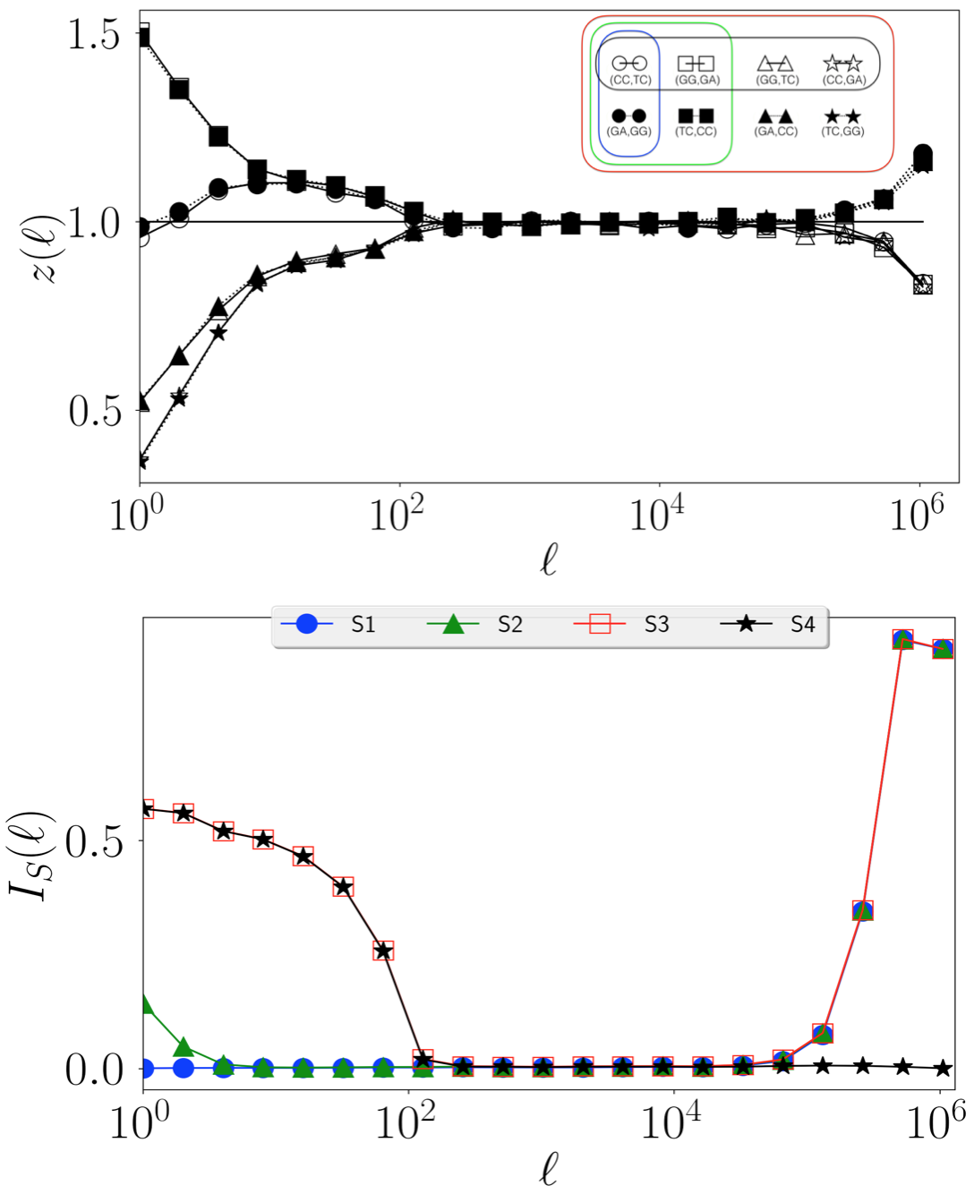
Deviations from $z=1$ are signatures of structure (correlations). Table 1 shows the results for chromosome 1 of Homo Sapiens, using a representative set of eight symmetrically related pairs of dinucleotides at a small scale $\ell=4$. The results show that $z$ is significantly different from one and that Chargaff symmetric observables $(Y,\hat{Y})$ appear with similar frequency, in agreement with conjecture (4). Figure 1 shows the same results of the Table varying logarithmically the scale $\ell$ from $\ell=1$ up to $\ell\simeq 10^{7}$ ( more precisely we use $\ell=2^{i}$ with $i\in\{0,1,2,..,24\}$). At different scales $\ell$ we see that a number of lines (observables $X_{A},X_{B}$) coincide with each other, reflecting the existence of different types of symmetries.

$X=X_{A}\;****\;X_{B}$	$P(X)$	$z_{[X_{A},X_{B}]}(\ell=4)$
CC **** TC	0.00401	1.236
GA **** GG	0.00404	1.242
GG **** GA	0.00366	1.127
TC **** CC	0.00366	1.128
GG **** TC	0.00302	0.929
GA **** CC	0.00299	0.922
CC **** GA	0.00265	0.818
TC **** GG	0.00264	0.813

Table 1: Chargaff symmetric observables appear with similar frequency in the human chromosome $1$. Each line contains an observable $X$ constructed combining oligonucleotides $\alpha_{1}\alpha_{2}\ldots\alpha_{8}$ where $\alpha_{1}\alpha_{2}$ equal to $X_{A}$ , $\alpha_{3}\alpha_{4}\alpha_{5}\alpha_{6}$ are arbitrary (any in $\{A,C,T,G\}$), and $\alpha_{7}\alpha_{8}$ equal to $X_{B}$ . Observables related by the extended Chargaff symmetry (3) appear on top of each other (separated by an horizontal line). The frequency of each observable $P(X)$ was computed using Eq. (1) and the normalized version (cross correlation) $z_{[X_{A},X_{B}]}(\ell=4)$ using Eq. (5)

.

Figure 1: Symmetrically related cross-correlations in Homo Sapiens - Chromosome 1. The normalized cross-correlations $z_{[CC,TC]}(\ell)$ as a function of the scale $\ell$, together with that of its symmetrical related companions. Symmetries are significant also at scales where non trivial correlations are present $z\neq 1$.

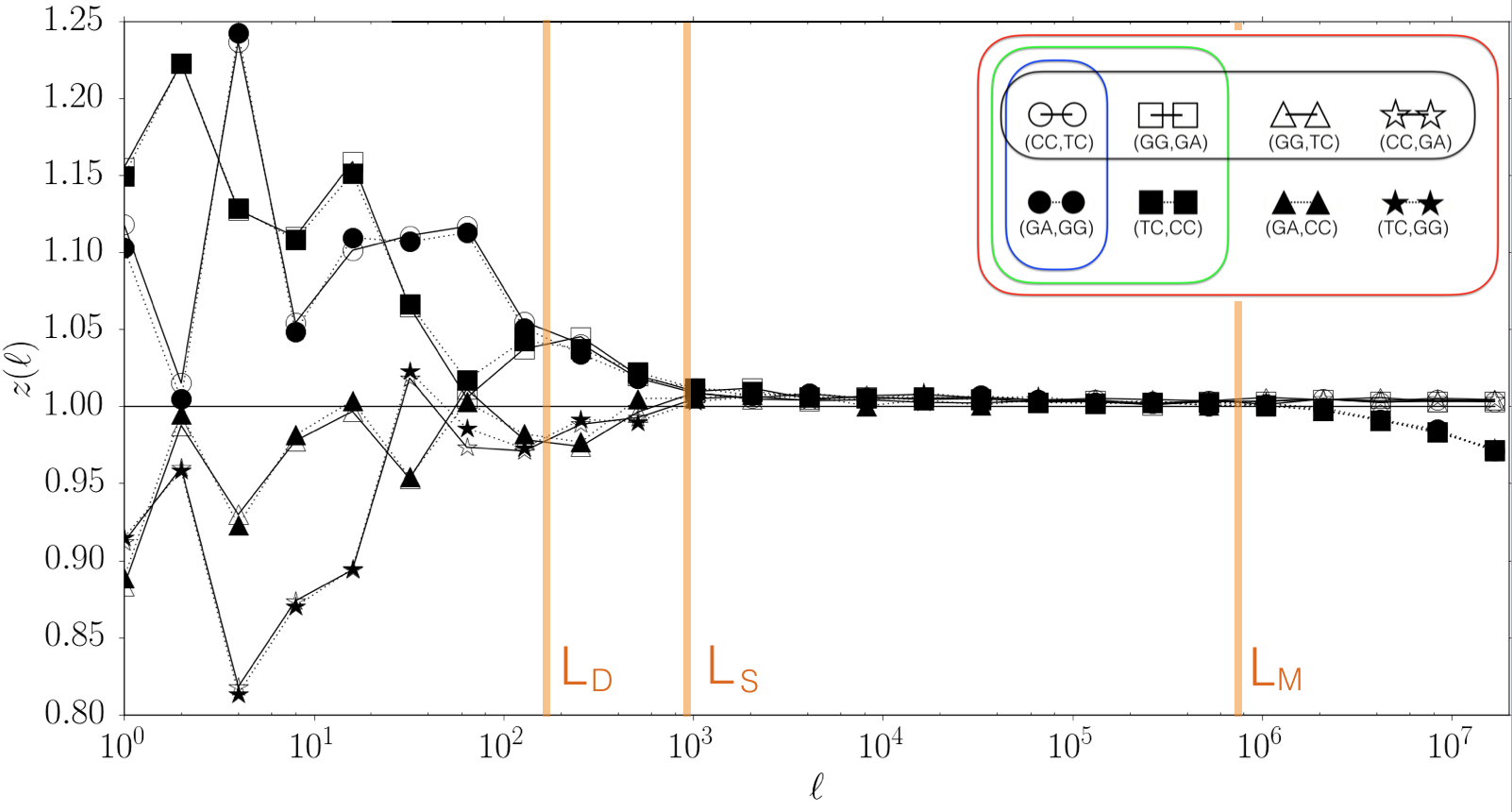
In order to understand the observations reported above it is necessary to formalize the symmetries that arise as composition of basic transformations. Starting from a reference observable $Y=(X_{A},X_{B};\ell)$, these symmetries are defined as compositions of the following two transformations:

• reverses the order in the pair: $(X_{A},X_{B};\ell)\xrightarrow{R}(X_{B},X_{A};\ell)$.

• applies our extended symmetry equation (3) to the first of the two observable in the pair: $(X_{A},X_{B};\ell)\xrightarrow{C}(\hat{X}_{A},{X}_{B};\ell)$.

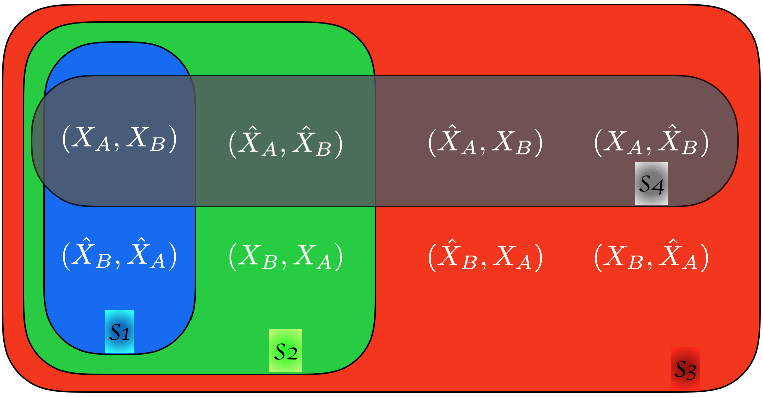
Note that $RC\neq CR$ (i.e. $R$ and $C$ do not commute), $RR=CC=Id$ (i.e. $R,C$ are involutions), and $CRC$ is the symmetry equivalent to equation (3). A symmetry $S$ is defined by a set of different compositions of $C$ and $R$. We denote by $\mathcal{S}_{S}(Y)$ the set of observables obtained applying to observable $Y$ all combinations of transformations in $S$. For example if $S1=\{CRC\}$ then $\mathcal{S}_{S1}(X_{A},X_{B};\ell)=\{(X_{A},X_{B};\ell),(\hat{X}_{B},\hat{X}_{A},\ell)\}$; if $S2=\{CRC,R\}$ then in addition to the set $\mathcal{S}_{S1}$ obtained from $CRC$ we should add the observables obtained by applying $R$ to every element of $\mathcal{S}_{S1}$, that are $R((X_{A},X_{B};\ell))=(X_{B},X_{A};\ell)$ and $R((\hat{X}_{B},\hat{X}_{A},\ell))=(\hat{X}_{A},\hat{X}_{B},\ell)$ thus obtaining $\mathcal{S}_{S2}(X_{A},X_{B};\ell)=\{(X_{A},X_{B};\ell),(\hat{X}_{B},\hat{X}_{A},\ell),(X_{B},X_{A};\ell),(\hat{X}_{A},\hat{X}_{B},\ell)\}$. The four symmetries we consider here are shown in Fig. 2 and correspond to: $S1$ (blue, obtained from $\{CRC\}$ and corresponding to the extended Chargaff (4)), $S2$ (green, obtained from $\{CRC,R\}$), $S3$ (red, obtained from $\{R,C\}$), and $S4$ (black, obtained from $\{RCR,C\}$). We can now come back to Fig. 1 and interpret the observations as follows: at scales $\ell<L_{D}$ curves are significantly different from $z=1$ and appear in pairs (same symbol, symmetry $S1$) which almost coincide even in the seemingly random fluctuations; around $\ell\simeq L_{D}\approx 2\;10^{2}$ two pairs merge forming two groups of four curves each (symmetry $S2$). At larger scales $\ell\geq L_{S}\approx 10^{3}$ all curves coincide (symmetry $S3$) at $z\approx 1$ (no structure). At very large scales $\ell>L_{M}\approx 10^{6}$ two groups of four observables separate (symmetry $S4$). Similar results are obtained for all choice of dinucleotides and for all chromosomes (see SI: Supplementary data [42]). These results suggest that: (i) the extended Chargaff symmetry we conjectured in Eq. (4) is valid up to a critical scale $L_{M}\simeq 10^{6}$; (ii) there are other characteristic scales connected to the other symmetries.

Figure 2: Sets of symmetrically related observables. Starting from a reference observable $Y=(X_{A},X_{B},\ell)$, the different colors illustrate the nested sets related by symmetries $S1-S4$. The symmetries shown in the figure correspond to: $S1$ (blue, obtained from $\{CRC\}$), $S2$ (green, obtained from $\{CRC,R\}$), $S3$ (red, obtained from $\{R,C\}$), and $S4$ (black, obtained from $\{RCR,C\}$).

The scale-dependent results discussed above motivate us to quantify the strength of validity of symmetries at different scale $\ell$. This is done computing for each symmetry $S$ an indicator $I_{S}(\ell)$ that measures the distance between the curves $z(\ell)$ of symmetry-related pairs $(X_{A},X_{B})$ and compares this distance to the ones that are not related by $S$. More precisely, for a given reference pair $Y_{\textrm{ref}}=(X_{A},X_{B})$ and symmetry $S\in\{S1,S2,S3,S4\}$, we consider the following distance of $Y_{\textrm{ref}}$ to the set $\mathcal{S}_{S}$ of observables obtained from symmetry $S$:

$$d_{\ell}(Y_{\textrm{ref}};S) := \frac{1}{|\mathcal{S}_{S}|}{\sum}_{Y\in\mathcal{S}_{S}(Y_{\textrm{ref}})}{\frac{\left[z_{[Y]}{(\ell)}-z_{[Y_{\textrm{ref}}]}(\ell)\right]^{2}}{\sigma^{2}(\ell)}}$$ (6)

where $\sigma(\ell)$ denotes the standard deviation of $z(\ell)$ over all $Y$. We then average over the set $\mathcal{A}$ of all $Y_{\textrm{ref}}$ (all possible pairs $X_{A},X_{B}$) to obtain a measure of the strength of symmetry $S$ at scale $\ell$ given by

$$I_{S}(\ell):=\frac{1}{2|\mathcal{A}|}{\sum}_{Y_{\textrm{ref}}\in\mathcal{A}}{d_{\ell}(Y_{\textrm{ref}};\mathcal{S})}$$ (7)

Note that $I_{S}(\ell)=0$ indicates full validity of the symmetry $S$ at the scale $\ell$ ($z$ is the same for all $Y$ in $\mathcal{S}$) and $I_{S}(\ell)=1$ indicate that $S$ is not valid at scale $\ell$ ($z$ varies in $\mathcal{S}$ as much as it varies in the full set).

Figure 3: Hierarchy of symmetries in Homo Sapiens - Chromosome 1. [ Upper panel ] The symmetry index $I_{S}(\ell)$ as a function of the scale $\ell$, the smaller the value the larger the importance of the symmetry. [Bottom panel ] The color bars helps visualise the onset of the different symmetries: symmetry is considered present if $0\leq I_{S}\leq 0.025$ and bar is (linearly interpolated) from full color to white, correspondingly.

Figure 4: Hierarchy of symmetries in Homo Sapiens. - All chromosomes. The symmetry index $I_{S}(\ell)$ as a function of the scale $\ell$ for the full set of chromosomes in Homo Sapiens. The brighter the color, the larger is the relevance of the symmetry $S_{1},S_{2},S_{3},$ or $S_{4}$ (more precisely, if $I_{min}$ is the minimum $I_{S}$ in each chromosome, $I_{S}\leq 1.05I_{min}$ is set to full color, $I_{S}\geq 6.5I_{min}$ is set to white, with intermediate values interpolated between these extremes.)

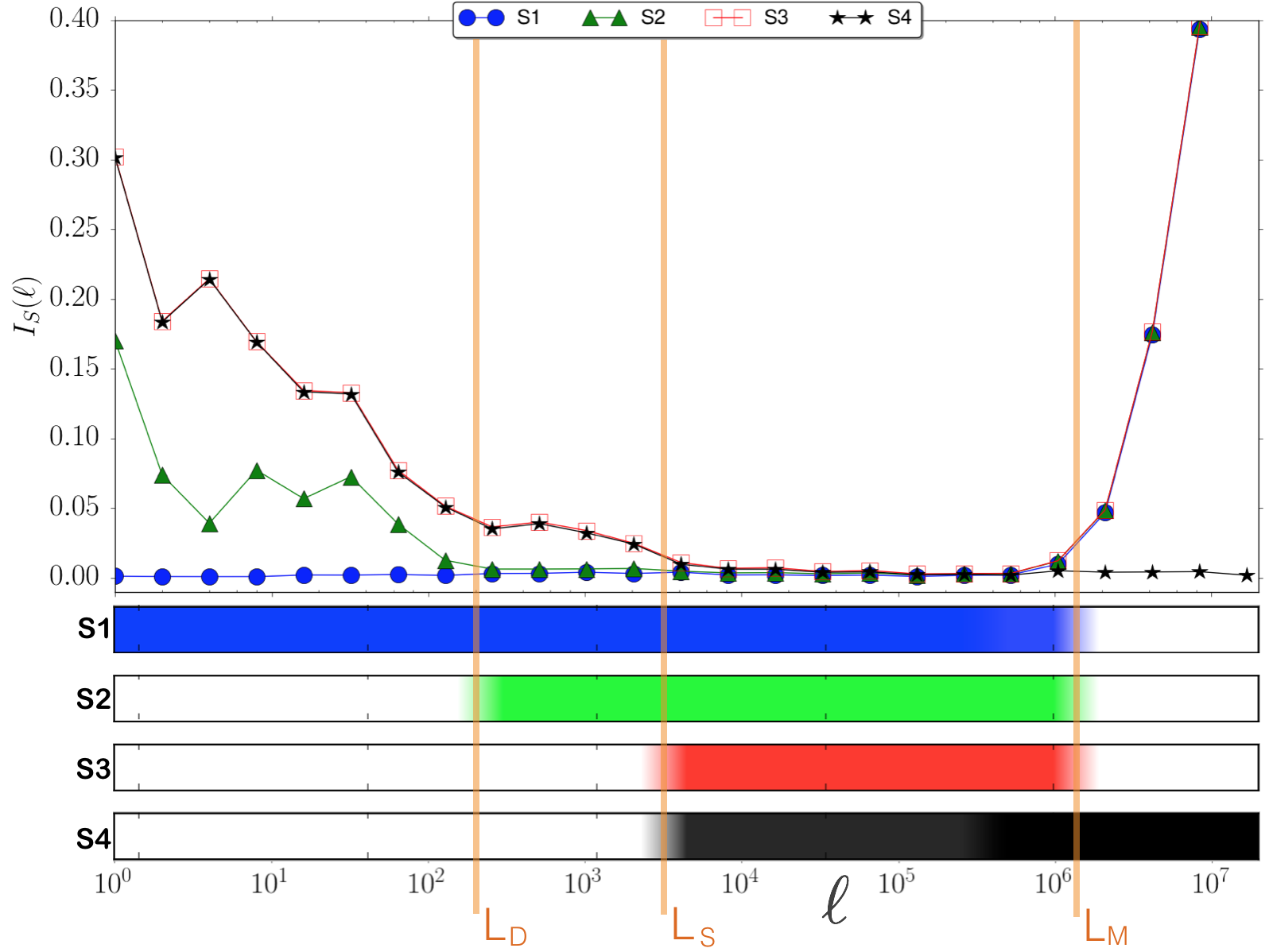
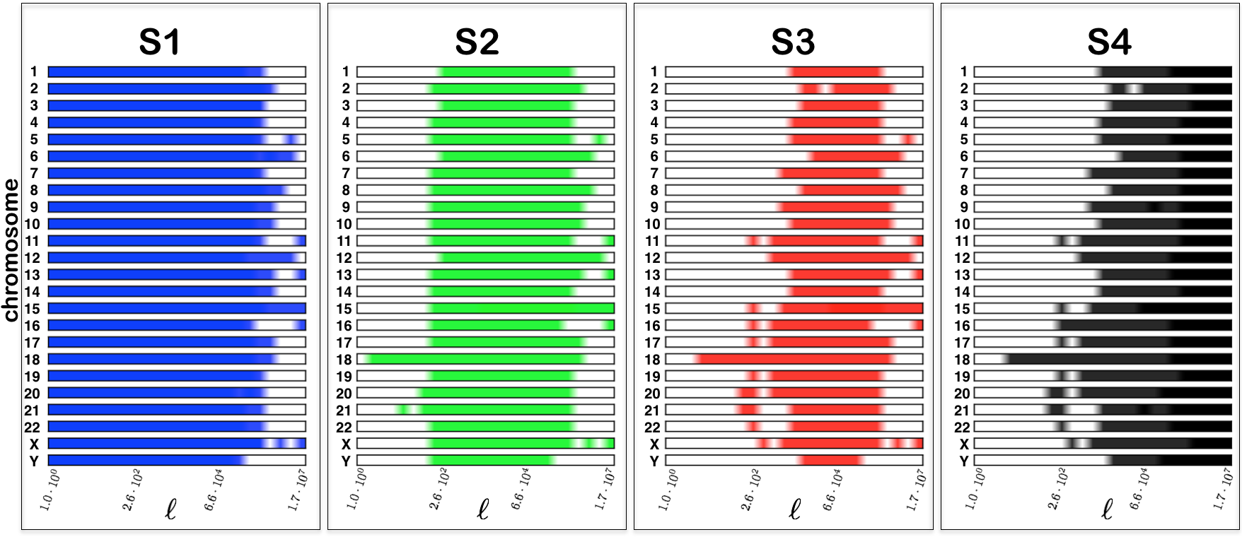
Figure 3 shows the results for chromosome 1 and confirms the existence of a hierarchy of symmetries at different structural scales. The estimated relevant scales in chromosome 1 (of total length $N\approx 2\times 10^{8}$) are $L_{D}\approx 10^{2}$, $L_{S}\approx 10^{3}$, and $L_{M}\approx 10^{6}$. Note that $L_{D}$ and $L_{M}$ are compatible with the known average-size of transposable elements and isochores respectively [31, 32]. Moreover, the results for all Homo-Sapiens chromosomes, summarised in Fig.4, show that not only the hierarchy is present, but also that the scales $L_{D},L_{S},$ and $L_{M}$ are comparable across chromosomes. This remarkable similarity (see also [37, 38, 39]) suggests that some of the mechanisms shaping simultaneously structure and symmetry work similarly in every chromosomes and/or act across them (e.g.chromosome rearrangements mediated by transposable elements). This, and the scales of $L_{D},L_{S}$, and $L_{M}$, provide a hint on the origin of our observations, which we explore below through the proposal of a minimal model.

A minimal model

We construct a minimal domain model for DNA sequences s that aims to explain the observations reported above. The key ingredient of our model is the reverse-complement symmetry of domain-types, suggested by the fact that transposable elements act on both strands. Mobile elements are recognised to play a central role in shaping domains and other structures up to the scale of a full chromosome, as well as being considered responsible for the appearance of Chargaff symmetry[29]. Our model accounts for structures (e.g., the patchiness and long-range correlations in DNA) in a similar way as other domain models do, the novelty is that it shows the consequences to the symmetries of the full DNA sequence.

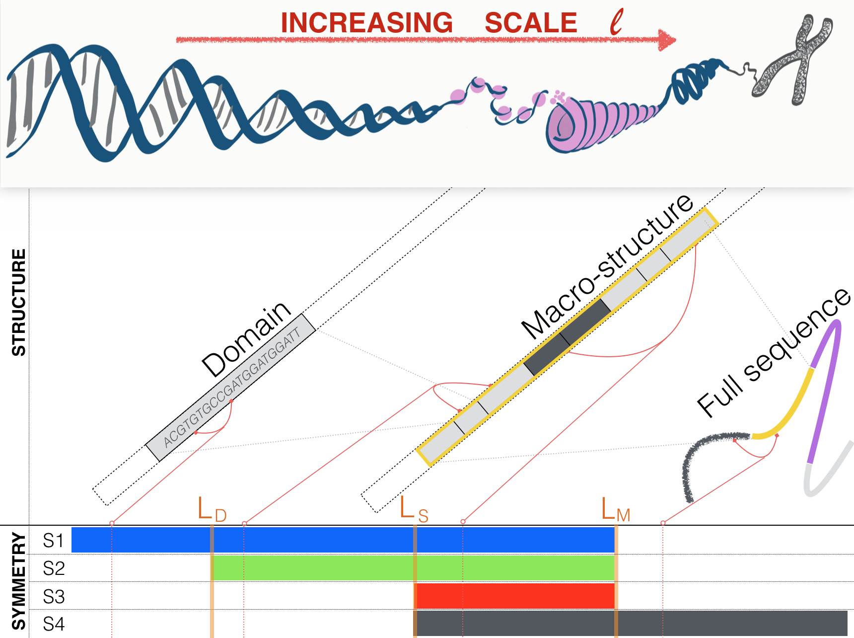
Motivated by our finding of the three scales $L_{D},L_{S},$ and $L_{M}$, our model contains three key ingredients at different length scales $\ell$ (see Fig.5 for an illustration):

Figure 5: Structure and symmetry at different scales: domain model. Structure and symmetry at different scales $\ell$ of genetic sequences can be explained using a simple domain model. Our model considers that the full sequence is composed of macro-structures (of size $L_{M}$) made by the concatenation of domains (of average size $L_{D}<L_{M}$), which are themselves correlated with neighbouring domains (up to a scale $L_{D}<L_{S}<L_{M}$). The biological processes that shapes domains imposes that, in each macrostructure, the types of domains comes in symmetric pairs. As a consequence, we show that four different symmetries $S_{1}-S_{4}$ are relevant at different scales $\ell$ (see text for details).

• at small scales, a genetic sequence $\textbf{d}=\alpha_{1}\alpha_{2}\cdots\alpha_{n}$ (of average size $\langle n\rangle\approx L_{D}$ ) is generated as a realization of a given process $p$. We do not impose a priori restrictions or symmetries on this process. We consider that one realization of this process builds a domain of type $p$. For a given domain type, the symmetrically related type is defined by the process $\hat{p}$ as follows: take a realization ($\alpha_{1}\alpha_{2}\ldots\alpha_{n}$) of the process $p$, revert its order $(\alpha_{n}\alpha_{n-1}\ldots\alpha_{1})$, and complement each base $(\hat{\alpha}_{n}\hat{\alpha}_{n-1}\ldots,\hat{\alpha}_{1})$, where $\hat{A}=T,\hat{T}=A,\hat{C}=G,\hat{G}=C$;

• at intermediate scales, a macro-structure is composed as a concatenation of domains $\textbf{d}_{1}\textbf{d}_{2}\cdots\textbf{d}_{m}$ (of average size $\langle m\rangle\approx L_{M}$), each domain belonging to one of a few types. We assume that symmetrical related domains (generated by $p$ and $\hat{p}$) appear with the same relative abundance and size-distribution in a given macro-structure. The concatenation process is done so that domains of the same type tend to form clusters of average size $L_{S}$ such that $L_{D}<L_{S}\ll L_{M}$;

• at large scales $(\gg L_{M})$, the full genetic sequence is composed by concatenations of macro-structures, each of them governed by different processes and statistics (e.g. different CG content [13, 14]).

Figure 6: Hierarchy of symmetries in a synthetic sequence generated by the domain model. The analysis of a synthetic genetic sequence generated by our model reproduces the hierarchy of symmetries observed in the human genome (compare the two panels to Figs. 1 and 3). The synthetic sequence is obtained following steps (1)-(3) of the main text. As main stochastic processes $p$ we use Markov chains with invariant probabilities $\mu$ such that $\mu(A)\neq\mu(T)$ and $\mu(C)\neq\mu(G)$ (no symmetries) (see Materials for details).

Statistical properties of the model and predictions

We now show how the model proposed above accounts for our empirical observation of a nested hierarchy of four symmetries $S_{1}$-$S_{4}$ at different scales. We start generating a synthetic sequence for a particular choice of parameters of the model described above (see section Methods for details). Figure 6 shows that such synthetic sequence reproduces the same hierarchy of symmetries we detected in Homo Sapiens.

We now argue analytically why these results are expected. The key idea is to note that for different separations $\ell$ (between the two observables $X_{A}$ and $X_{B}$) different scales of the model above dominate the counts used to compute $P(X_{A},X_{B};\ell)$ through Eq. (1) (see Supplementary Information for a more rigorous derivation):

• ($\ell\ll L_{D}$): $P(X_{A},X_{B},\ell)$ is dominated by $X_{A}$ and $X_{B}$ in the same domain. As domain-types appear symmetrically in each macro-structure, $P(X_{A},X_{B};\ell)=P(\hat{X}_{B},\hat{X}_{A};\ell)$. This is compatible with the conjecture (4).
  
  $S1=\{CRC\}$
  $\mathcal{S}_{S1}=\{(X_{A},X_{B};\ell),(\hat{X}_{B},\hat{X}_{A};\ell)\}$.
  

• ($L_{D}\ll\ell\ll L_{S}$): $P(X_{A},X_{B},\ell)$ is dominated by $X_{A}$ and $X_{B}$ in different domains. As domains are independent realizations, the order of $X_{A}$ and $X_{B}$ becomes irrelevant and therefore $R$ becomes a relevant symmetry (in addition to $CRC$). If domains of the same type tend to cluster, then for $L_{D}<\ell\ll L_{S}$ the main contribution to $P(X_{A},X_{B},\ell)$ comes from $X_{A}$ and $X_{B}$ in different domains of the same type (i.e., on different realizations of the same process $p$).
  
  $S2=\{CRC,R\}$
  $\mathcal{S}_{S2}=\{(X_{A},X_{B};\ell),(\hat{X}_{B},\hat{X}_{A};\ell),(X_{B},X_{A};\ell),(\hat{X}_{A},\hat{X}_{B};\ell)\}$.

  Note that $\mathcal{S}_{S1}\subset\mathcal{S}_{S2}$.
  

• ($L_{S}\ll\ell\ll L_{M}$): $P(X_{A},X_{B},\ell)$ is dominated by $X_{A}$ and $X_{B}$ in different domains inside the same macro-structure. For $\ell>L_{S}$ the domains of $X_{A}$ and $X_{B}$ of different types can be considered independent form each other. Therefore, in addition to the previous symmetries, $C$ is valid.
  
  $S3=\{R,C\}$
  $\mathcal{S}_{S3}=\{(X_{A},X_{B};\ell),(\hat{X}_{B},\hat{X}_{A};\ell),(X_{B},X_{A};\ell),(\hat{X}_{A},\hat{X}_{B};\ell),\\ (X_{A},\hat{X}_{B};\ell),(\hat{X}_{A},X_{B};\ell),(X_{B},\hat{X}_{B};\ell),(\hat{X}_{B},X_{A};\ell)\}$.

  Note that $\mathcal{S}_{S1}\subset\mathcal{S}_{S2}\subset\mathcal{S}_{S3}$.
  

• ($\ell\gg L_{M}$): $P(X_{A},X_{B},\ell)$ is dominated by $X_{A}$ and $X_{B}$ in different macro-structures. Note that the frequency of $X_{A}$ in one macro-structure and $\hat{X}_{A}$ in a different macro-structure are, in general, different. Therefore, for generic $X_{A},X_{B}$ we have $P(X_{A},X_{B};\ell)\neq P(\hat{X}_{B},\hat{X}_{A};\ell)$, meaning that $S1$ (and thus $S2$ and $S3$) is no longer valid. On the other hand, our conjectured Chargaff symmetry, Eq. (4), is valid for both $X_{A}$ and $X_{B}$ separately (because they are small scale observables). Therefore $X_{A}$ and $X_{B}$ can be interchanged in the composite observable $Y$.
  $S4=\{RCR,C\}$
  $\mathcal{S}_{S4}=\{(X_{A},X_{B};\ell),(\hat{X}_{A},{X_{B}};\ell),({X_{A}},\hat{X}_{B};\ell),(\hat{X}_{A},\hat{X}_{B};\ell)\}$.

  Note that $\mathcal{S}_{S4}\subset\mathcal{S}_{S3}$.

Discussion

The complement symmetry in double-strand genetic sequences, known as the First Chargaff Parity Rule, is nowadays a trivial consequence of the double-helix assembly of DNA. However, from a historical point of view, the symmetry was one of the key ingredients leading to the double-helix solution of the complicated genetic structure puzzle, demonstrating the fruitfulness of a unified study of symmetry and structure in genetic sequences. In a similar fashion, here we show empirical evidence for the existence of new symmetries in the DNA (Figs. 1-4) and we explain these observations using a simple domain model whose key features are dictated by the role of transposable elements in shaping DNA. In view of our model, our empirical results can be interpreted as a consequence of the action of transposable elements that generate a skeleton of symmetric domains in DNA sequences. Since domain models are known to explain also much of the structure observed in genetic sequences, our results show that structural complex organisation of single-strand genetic sequences and their nested hierarchy of symmetries are manifestations of the same biological processes. We expect that future unified investigations of these two features will shed light into their (up to now not completely clarified) evolutionary and functional role. For this aim, it is crucial to extend the analyses presented here to organisms of different complexity [23]. In parallel, we speculate that the unraveled hierarchy of symmetry at different scales could play a role in understanding how chromatin is spatially organised, related to the puzzling functional role of long-range correlations [40, 41].

Methods

Algorithm used to generate the synthetic sequence

We create synthetic genetic sequences through the following implementation of the three steps of the model we proposed above:

• The processes $p$ we use to generate genetic sequences are Markov processes of order one such that the nucleotide $s_{i}$ at position $i$ is drawn from a probability $P(s_{i}|s_{i-1})=M_{s_{i-1},s_{i}}$, where $M$ is a $4$ by $4$ stochastic matrix. The matrices $M$ are chosen such that the processes’ invariant measures $\mu$ do not satisfy the Chargaff property: $\mu(A)\neq\mu(T)$ and $\mu(C)\neq\mu(G)$. The exponential decay of correlations of the Markov chains determines the domain sizes $L_{D}$ (in our case $L_{D}\simeq 10$).

• We use the processes $p$ to generate chunks of average size $150$ (the length of each chunck was drawn uniformly in the range $[130,170]$. With probability $1/2$, we applied the reverse-complement (CRC) operation to the chunck before concatenating it to the previous chunck (process $\hat{p}$). This choice implies that the typical cluster size is $L_{S}\simeq 2*150=300$. The process of concatenating chunks together is repeated to form a macrostructure of length $L_{M}\simeq 10^{6}$.

• We concatenate two different macrostructures, obtained from steps (1) and (2) with two different matrices $M_{I}$ and $M_{II}$:

  $$M_{I}=\begin{bmatrix}0.2&0.1&0.2&0.5\\ 0.01&0.84&0.01&0.14\\ 0.4&0.1&0.4&0.1\\ 0.3&0.15&0.25&0.3\end{bmatrix},\;M_{II}=\begin{bmatrix}0.1&0.2&0.1&0.6\\ 0.1&0.75&0.1&0.05\\ 0.1&0.4&0.1&0.4\\ 0.1&0.35&0.45&0.1\end{bmatrix}$$

  where columns (and rows) corresponds to the following order: $[A,C,G,T]$.

Data handling

Genetic sequences of Homo Sapiens were downloaded from the National Center for Biotechnology Information $(ftp://ftp.ncbi.nih.gov/genomes/H\_sapiens)$. We used reference assembly build 38.2. The sequences were processed to remove all letters different from $A,C,G,T$ (they account for $\approx 1.66\%$ of the full genome and thus their removal has no significant impact on our results).

Codes

Ref. [42] contains data and codes that reproduce the figures of the manuscript for different choices of observables and chromosomes.

Author contributions statement

G.C. initiated and designed the study. E.G.A. and G.C. contributed to the development of the study, carried out statistical analysis and wrote the manuscript. E.G.A , G.C. and M.D.E. discussed and interpreted the results. E.G.A , G.C. and M.D.E reviewed the manuscript.

Additional information

Competing interests The authors declare that they have no competing interests.

Supplementary Information

Derivation of the nested hierarchy of symmetries

We derive the nested hierarchy of symmetries in the minimal model for genetic sequence.

Notation and model properties

To fix notations, we describe our model and its statistical properties as follows:

• The full sequence is build concatenating $r$ macro-structures: $\textbf{s}=\textbf{m}_{1}\,\textbf{m}_{2}\cdots\textbf{m}_{r}$.

• A macrostructure m is build concatenating $m$ domains: $\textbf{m}=\textbf{d}^{\textbf{\tiny m}}_{1}\,\textbf{d}^{\textbf{\tiny m}}_{2}\cdots\textbf{d}^{\textbf{\tiny m}}_{m}$.

• The average domain length is denoted by $L_{D}$, the average macro-structure length is denoted by $L_{M}$. The total length of the sequence is $N$.

• A domain $\textbf{d}^{\textbf{\tiny m}}$ in the macro-structure m is a finite-size realisation of a process chosen between two symmetrically related process-types: $C_{\textbf{\tiny m}}$ and $\hat{C}_{\textbf{\tiny m}}$. We use the notation $\textbf{d}\in C$ to indicate that d is generated by the process of type $C$.

• For a a given observable X, we denote by $f_{C}(X)$ the limiting relative frequency of occurrence of $X$ in a domain of type $C$. Recall that, the definition of symmetrically related processes (of the same macro-structure) imposes that, for every choice of $X$:

  $$f_{C}(X)=f_{\hat{C}}(\hat{X})$$ (8)

  In principle, different macro-structures have different process-types statistics.

• We denote by $(\underline{c},\underline{l})$ an ordered sequence of domains of types $\underline{c}:=(c_{1},\cdots,c_{k});\quad c_{j}\in\{C,\hat{C}\}$ of lengths $\underline{l}:=(l_{1},\cdots,l_{k})$ respectively; and by $\hat{(\underline{c},\underline{l})}$ the sequence of domains defined by $(\hat{c}_{k},\cdots,\hat{c}_{1})$ and $(l_{k},\cdots,l_{1})$. We denote by $\pi^{\textbf{\tiny m}}[(\underline{c},\underline{l})]$ the relative frequency of counts of subsequence of domains $(\underline{c},\underline{l})$ in m.
  

  We denote by $\pi^{\textbf{\tiny m}}(\{c,l\})$ the relative frequency of a cluster of length $l$ of domains of the same type $c$.
  For $\alpha,\beta\in\{C,\hat{C}\}$ and $k\geq 1$ , we denote $\pi^{\textbf{\tiny m}}(\alpha,\beta;k)$ the relative frequency of $j$ such that $\textbf{d}_{j}\in\alpha$ and $\textbf{d}_{j+k}\in\beta$.
  

• In each macro-structure, the probability distribution of domain-sizes is denoted $p_{\textbf{\tiny m}}(l)$.

• We do not enforce any prescription to concatenate domains in a macrostructure (determined by $\pi$), but the following properties:

  • $\pi^{\textbf{\tiny m}}[(\underline{c},\underline{l})]=\pi^{\textbf{\tiny m}}[\hat{(\underline{c},\underline{l})}]$ This ensure that the structural statistics of two symmetrically coupled domain-types ordering is unbiased.

  • for $k>>L_{S}/L_{D}$ ; $\pi^{\textbf{\tiny m}}(c_{1},c_{2},k)=\pi^{\textbf{\tiny m}}(c_{1})\pi^{\textbf{\tiny m}}(c_{2})$. This defines the average length $L_{S}$ beyond which correlations in domain ordering can be neglected. $L_{S}$ is thus the average size of clusters of domains of the same type.

Derivation of symmetries

We start by showing the validity of the extended Chargaff symmetry $P(X)=P(\hat{X})$ for $\ell<L_{M}$. We denote by $\#_{(\underline{c},\underline{l})}(X)$ the counts of $X$ inside $(\underline{c},\underline{l})$. Using $\pi[(\underline{c},\underline{l})]=\pi[\hat{(\underline{c},\underline{l})}]$ and $f_{C}(X)=f_{\hat{C}}(\hat{X})$ we have that $\#_{(\underline{c},\underline{l})}(X)=\#_{\hat{(\underline{c},\underline{l})}}(\hat{X})$. Finally, for $X$ of size $\ell_{X}\ll L_{M}$, the counts of $X$ in the full sequence is dominated by $X$ not overlapping different macro-structures and thus we conclude that ($N^{\prime}=N-\ell$)

$$P(X) \simeq 1/N^{\prime}\sum_{m}\sum_{(\underline{c},\underline{l})_{m}}\#_{(\underline{c},\underline{l})}(X)$$ (9)

$$= 1/N^{\prime}\sum_{m}\sum_{\hat{(\underline{c},\underline{l})}_{m}}\#_{\hat{(\underline{c},\underline{l})}}(\hat{X})$$

$$\simeq P(\hat{X}).$$

We now show the validity of the nested hierarchy of symmetries discussed in the main paper. We focus on observables of the form $Y=(X_{A},X_{B};\ell)$, where $X_{A}$ and $X_{B}$ are oligonucleotide of size much smaller than typical domain sizes $L_{D}$. We always approximate the counts of $X$ inside a domain of type $C$ and of length $l$ by $l\cdot f_{C}(X)$.

Define

$$\#_{(i)}(Y) := Y i$$ number of fully inside the -th domain

$$\#_{(ij)}(X_{A},X_{B},\ell) := X_{A} i X_{B} j \ell$$ number of fully in the -th and in the -th domains, at distance

$$\#(Y) := Y:=(X_{A},X_{B},\ell)$$ number of in the full string

$$= \sum_{i}\#_{(i)}(Y)+\sum_{i}\sum_{j>i}{\#_{(ij)}(X_{A},X_{B},\ell)}+$$

$$+\{\textrm{terms where $X_{A}$ or $X_{B}$ overlap domains boundaries}\}$$

As we will consider only the case $l_{X_{A}},l_{X_{B}}\ll L_{D}$, we neglect the last term.

We can now investigate and rule out the main contributions to the overall counting $\#(Y)$ at different scales:

• $(\ell\ll L_{D})$: At these scales the following sum dominates,

  $$\#(Y)\simeq\sum_{i=1}\#_{(i)}(Y) \simeq \sum_{m=1}^{r}g_{m}(\ell)\left[f_{C_{\textbf{\tiny m}}}(Y)+f_{\hat{C}_{\textbf{\tiny m}}}(Y)\right]$$

  $$= \sum_{m=1}^{r}g_{m}(\ell)\left[f_{C_{\textbf{\tiny m}}}(Y)+f_{C_{\textbf{\tiny m}}}(\hat{Y})\right]$$

  where

  $$g_{m}(\ell):=\frac{1}{2}\sum_{l=\ell}^{\infty}p_{m}(l)(l-\ell)\quad\quad\quad\ell\ll L_{D}.$$

  
  

  We conclude that $\#(X_{A},X_{B},\ell)\simeq\#(\hat{X}_{B},\hat{X}_{A},\ell)$ at these scales, and thus symmetry $S1$ is valid. This can also be derived directly from equation (9).

For $\ell>>L_{D}$, $X_{A}$ and $X_{B}$ typically lie in different domains and therefore the second term in equation (Derivation of symmetries) dominates

$$\#(Y)\simeq\sum_{i=1}\sum_{j>i}{\#_{(ij)}(X_{A},X_{B},\ell)}.$$

The counts will be estimated as the product of the probabilities of $X_{A}$ and $X_{B}$ because each domain is an independent realisations. At different scales $\ell$ there are different relationships between the domains in which $X_{A}$ and $X_{B}$ typically lie, leading to the following cases:

• $(L_{D}<<\ell<L_{S})$: At these scales the sum is dominated by counts of $Y$ inside a cluster of domains of the same type. Each cluster contribute to the counts of $Y$ with a term $\pi[\{c,l\}](l-\ell)f_{C}(X_{A})f_{C}(X_{B})$ and thus, in this case

  $$\sum_{i=1}\sum_{j>i}{\#_{(ij)}(X_{A},X_{B},\ell)} \simeq \sum_{m=1}^{r}h_{m}(\ell)\left[f_{C_{\textbf{\tiny m}}}(X_{A})f_{C_{\textbf{\tiny m}}}(X_{B})+f_{\hat{C}_{\textbf{\tiny m}}}(X_{A})f_{\hat{C}_{\textbf{\tiny m}}}(X_{B})\right]$$

  $$= \sum_{m=1}^{r}h_{m}(\ell)\left[f_{C_{\textbf{\tiny m}}}(X_{A})f_{C_{\textbf{\tiny m}}}(X_{B})+f_{C_{\textbf{\tiny m}}}(\hat{X}_{A})f_{C_{\textbf{\tiny m}}}(\hat{X}_{B})\right]$$

  where

  $$h_{m}(\ell):=\frac{1}{2}\sum_{l=\ell}^{\infty}\pi[\{c,l\}](l-\ell)\quad\quad\quad L_{D}<\ell\ll L_{S}$$

  
  

  We conclude that $\#(X_{A},X_{B},\ell)\simeq\#(\hat{X}_{B},\hat{X}_{A},\ell)\simeq\#(X_{B},X_{A},\ell)\simeq\#(\hat{X}_{A},\hat{X}_{B},\ell)$ at these scales, and thus symmetry $S2$ (and $S1$) is valid. If the processes are such that correlations inside domains vanishes at a scale smaller than the realization of the process, we consider this shorter correlation time to be the effective domain size $L_{D}$ and $S2$ sets in at this shorter scale.
  
  

• $(L_{S}\ll\ell\ll L_{M})$: At these scales the sum is dominated by $X_{A}$ and $X_{B}$ lying in different cluster

  $$\sum_{i}\sum_{j>i}{\#_{(ij)}(X_{A},X_{B},\ell)} = s(\ell)\sum_{m=1}^{r}\left[f_{C_{\textbf{\tiny m}}}(X_{A})f_{C_{\textbf{\tiny m}}}(X_{B})+f_{C_{\textbf{\tiny m}}}(X_{A})f_{\hat{C}_{\textbf{\tiny m}}}({X}_{B})+\right.$$

  $$\left.\quad\quad\quad\quad\quad+f_{\hat{C}_{\textbf{\tiny m}}}({X}_{A})f_{C_{\textbf{\tiny m}}}(X_{B})+f_{\hat{C}_{\textbf{\tiny m}}}({X}_{A})f_{\hat{C}_{\textbf{\tiny m}}}({X}_{B})\right]$$

  $$= s(\ell)\sum_{m=1}^{r}\left[f_{C_{\textbf{\tiny m}}}(X_{A})f_{C_{\textbf{\tiny m}}}(X_{B})+f_{C_{\textbf{\tiny m}}}(X_{A})f_{{C}_{\textbf{\tiny m}}}(\hat{X}_{B})+\right.$$

  $$\left.\quad\quad\quad\quad\quad+f_{{C}_{\textbf{\tiny m}}}(\hat{X}_{A})f_{C_{\textbf{\tiny m}}}(X_{B})+f_{{C}_{\textbf{\tiny m}}}(\hat{X}_{A})f_{{C}_{\textbf{\tiny m}}}(\hat{X}_{B})\right]$$

  $$= s(\ell)\sum_{m=1}^{r}\left[\left(f_{C_{\textbf{\tiny m}}}(X_{A})+f_{{C}_{\textbf{\tiny m}}}(\hat{X}_{A})\right)\left(f_{C_{\textbf{\tiny m}}}(X_{B})+f_{{C}_{\textbf{\tiny m}}}(\hat{X}_{B})\right)\right]$$

  where
  

  $$s(\ell)\simeq\frac{1}{4}(L_{M}-\ell)\quad\quad\quad L_{S}<\ell\ll L_{M}.$$

  
  

  We conclude that $\#(X_{A},X_{B},\ell)\simeq\#(\hat{X}_{B},\hat{X}_{A},\ell)\simeq\#(X_{B},X_{A},\ell)\simeq\#(\hat{X}_{A},\hat{X}_{B},\ell)\simeq\#(\hat{X}_{A},X_{B},\ell)\simeq\#(\hat{X}_{B},{X}_{A},\ell)\simeq\#(X_{B},\hat{X}_{A},\ell)\simeq\#({X}_{A},\hat{X}_{B},\ell)$ at these scales, and thus symmetry $S3$ (and $S2,S1$ and $S4$) is valid.

• $(L_{M}\ll\ell)$: At these scales the sum is dominated by counts where $X_{A}$ and $X_{B}$ are in different macro-structures:

  $$\sum_{i}\sum_{j>i}{\#_{(ij)}(X_{A},X_{B},\ell)} = \sum_{m=1}^{r}\sum_{n>m}q_{m,n}(\ell)\left[\left(f_{C_{\textbf{\tiny m}}}(X_{A})+f_{{\hat{C}}_{\textbf{\tiny m}}}({X}_{A})\right)\left(f_{C_{\textbf{\tiny n}}}(X_{B})+f_{\hat{C}_{\textbf{\tiny n}}}({X}_{B})\right)\right]$$

  $$= \sum_{m=1}^{r}\sum_{n>m}q_{m,n}(\ell)\left[\left(f_{C_{\textbf{\tiny m}}}(X_{A})+f_{{C}_{\textbf{\tiny m}}}(\hat{X}_{A})\right)\left(f_{C_{\textbf{\tiny n}}}(X_{B})+f_{{C}_{\textbf{\tiny n}}}(\hat{X}_{B})\right)\right].$$

  where $q_{m,n}(\ell)$ counts how many sites separated by $\ell$ lie in macro-structures m and n, respectively.
  We conclude that $\#(X_{A},X_{B},\ell)\simeq\#(\hat{X}_{A},X_{B},\ell)\simeq\#(X_{A},\hat{X}_{B},\ell)\simeq\#(\hat{X}_{A},\hat{X}_{B},\ell)$ and thus symmetry $S4$ is valid.

References

- [1] Peng, C.-K. et al. Long-range correlation in nucleotide sequences. Nature 356, 168-170 (1992).
- [2] Karlin S., Brendel V. Patchiness and correlations in DNA sequences. Science 259, 677-680 (1993).
- [3] Rudner R., Karkas J.D., Chargaff E. Separation of B. subtilis DNA into complementary strands I. Biological properties, II. Template functions and composition as determined, III Direct analysis. Proc. Natl. Acad. Sci. USA 60, 630-635; 915-922 (1968).
- [4] McClintock B. The significance of responses of the genome to challenge. Science 226, 792-801 (1984).
- [5] Fedoroff N.V. Transposable Elements, Epigenetics, and Genome Evolution. Science 338, 758-767 (2012).
- [6] Li W., Kaneko K. Long-Range Correlation and Partial Spectrum in a Noncoding DNA Sequence. EPL 17, 655-660 (1992).
- [7] Voss R. Evolution of Long-Range Fractal Correlations and Noise in DNA Base Sequences. Phys. Rev. Lett. 68, 3805-3808 (1992).
- [8] Amato I. DNA shows unexplained patterns writ large. Science 257, 747(1992).
- [9] Nee S. Uncorrelated DNA walks. Nature 357, 450 (1992).
- [10] Yam P. Noisy nucleotides: DNA sequences show fractal correlations. Sci. Am. 267, 23-24,27 (1992).
- [11] Li W., Marr T.G., Kaneko K. Understanding long-range correlations in DNA sequences. Physica D 75, 392-416 (1994).
- [12] Bryce R.M., Sprague K.B. Revisiting detrended fluctuation analysis. Sci. Rep. 2, 315 (2012).
- [13] Peng C.-K. et al. Mosaic organization of DNA nucleotides. Phys. Rev. E 49, 1685-1689 (1993).
- [14] Bernaola-Galván P., Román-Roldán R., Oliver J.L. Compositional segmentation and long-range fractal correlations in DNA sequences. Phys. Rev. E 53, 5181-5189 (1996).
- [15] Rogerson A.C. There appear to be conserved constraints on the distribution of nucleotide sequences in cellular genomes. J. Mol. Evol 32, 24-30 (1991).
- [16] Mitchell D., Bridge R. A test of Chargaff’s second rule Biochem. Biophys. Res. Commun. 340, 90-94 (2006).
- [17] Nikolaou C., Almirantis Y. Deviations from Chargaff’s second parity rule in organellar DNA Insights into the evolution of organellar genomes. Gene 381, 34-41 (2006).
- [18] Qi D., Cuticchia A.J. Compositional symmetries in complete genomes. Bioinformatics 17, 557-559 (2001).
- [19] Fickett J.W. , Torney D.C., Wolf D.R. Base compositional structure of genomes. Genomics 13, 1056-1064 (1992).
- [20] Prabhu V.V. Symmetry observations in long nucleotide sequences. Nucleic Acids Res. 21, 2797-2800 (1993).
- [21] Bell S.J., Forsdyke D.R. Accounting units in DNA. J. Theor. Biol. 197, 51-61 (1999).
- [22] Baisnée P.F., Hampson S., Baldi P. Why are complementary DNA strands symmetric? Bioinformatics 18, 1021-1033 (2002).
- [23] Kong S-G. et al. Inverse Symmetry in Complete Genomes and Whole-Genome Inverse Duplication. PLOS one 4, e7553 (2009).
- [24] Afreixo V. et al. The breakdown of the word symmetry in the human genome. J. Theor. Biol. 335, 153-1599 (2013).
- [25] Chargaff E. Structure and functions of nucleic acids as cell constituents. Fed. Proc. 10, 654-659 (1951).
- [26] Bell S.J., Forsdyke D.R. Deviations from Chargaff’s Second Parity Rule Correlate with Direction of Transcription. J. Theor. Biol. 197, 63-76 (1999).
- [27] Lobry J.R., Lobry C. Evolution of DNA base composition under no-strand-bias condition when the substitution rates are not constant. Mol. Biol. Evol. 16, 719-723 (1999).
- [28] Zhang S.H., Huang Y.Z. Limited contribution of stem-loop potential to symmetry of single-stranded genomic DNA. Bioinformatics 26, 478-485 (2010).
- [29] Albrecht-Buehler G. Asymptotically increasing compliance of genomes with Chargaff’s second parity rules through inversions and inverted transpositions. Proc. Natl. Acad. Sci. USA 103, 17828-17833 (2006).
- [30] Shporer S., Chor B., Rosset S., Horn D. Inversion symmetry of DNA k-mer counts: validity and deviations. BMC Genomics 17, 696 (2016).
- [31] Bernardi G. et al. The mosaic genome of warm-blooded vertebrates. Science 228 953-958 (1985).
- [32] Carpena P. , Bernaola-Galván P., Coronado A.V., Hackenberg M., Oliver J.L. Identifying characteristic scales in the human genome. Phys. Rev. E 75, 032903 (2007).
- [33] Li W. The Study of Correlation Structures of DNA Sequences: A Critical Review. Comput. Chem. 21, 257-71 (1987).
- [34] Afreixo V., Bastos C.A., Pinho A.J., Garcia S.P., Ferreira P.J. Genome analysis with inter-nucleotide distances. Bioinformatics 25, 3064-3070 (2009).
- [35] Frahm K.M., Shepelyansky D.L. Poincaré recurrences of DNA sequence. Phys. Rev. E 85, 016214 (2012).
- [36] Tavares A.H.M.P. et al. DNA word analysis based on the distribution of the distances between symmetric words. Sci. Rep. 7, 728 (2017).
- [37] Li W., Stolovitzky G., Bernaola-Galván P., Oliver J.L. Compositional Heterogeneity within, and Uniformity between, DNA Sequences of Yeast Chromosomes. Genome Res. 8, 916-928 (1998).
- [38] Forsdyke D.R., Zhang C., Wei J-F. Chromosomes as interdependent accounting units: the assigned orientation of C. Elegans chromosomes minimize the total W-base Chargaff difference. J. Biol. Syst. 18, 1-16 (2010).
- [39] Bogachev M.I., Kayumov A.R., Bunde A. Universal Internucleotide Statistics in Full Genomes: A Footprint of the DNA Structure and Packaging? PLoS ONE 9, e112534 (2014).
- [40] Bechtel J.M. et al. Genomic mid-range inhomogeneity correlates with an abundance of RNA secondary structures. BMC Genomics 9,284 (2008).
- [41] Arneodo A. et al. Multi-scale coding of genomic information: From DNA sequence to genome structure and function. Phys. Rep. 498, 45-188 (2011).
- [42] Altmann E. G., Cristadoro, G., Degli Esposti, M. (2017). Cross-correlations and symmetries in genetic sequences [Data set]. Zenodo 1001805 (2017), http://doi.org/10.5281/zenodo.1001805
Acknowledgements
EGA and GC thank the Max Planck Institute for the Physics of Complex Systems in Dresden (Germany) for hospitality and support at the early stages of this project.