On the Sample Complexity of the Linear Quadratic Regulator

Sarah Dean, Horia Mania, Nikolai Matni, Benjamin Recht, and Stephen Tu
University of California, Berkeley
\dagger California Institute of Technology
(October 3, 2017, Revised: )
Abstract

This paper addresses the optimal control problem known as the Linear Quadratic Regulator in the case when the dynamics are unknown. We propose a multi-stage procedure, called Coarse-ID control, that estimates a model from a few experimental trials, estimates the error in that model with respect to the truth, and then designs a controller using both the model and uncertainty estimate. Our technique uses contemporary tools from random matrix theory to bound the error in the estimation procedure. We also employ a recently developed approach to control synthesis called System Level Synthesis that enables robust control design by solving a quasiconvex optimization problem. We provide end-to-end bounds on the relative error in control cost that are optimal in the number of parameters and that highlight salient properties of the system to be controlled such as closed-loop sensitivity and optimal control magnitude. We show experimentally that the Coarse-ID approach enables efficient computation of a stabilizing controller in regimes where simple control schemes that do not take the model uncertainty into account fail to stabilize the true system.

1 Introduction

Having surpassed human performance in video games [42] and Go [51], there has been a renewed interest in applying machine learning techniques to planning and control. In particular, there has been a considerable amount of effort in developing new techniques for continuous control where an autonomous system interacts with a physical environment [17, 35]. A tremendous opportunity lies in deploying these data-driven systems in more demanding interactive tasks including self-driving vehicles, distributed sensor networks, and agile robotics. As the role of machine learning expands to more ambitious tasks, however, it is critical these new technologies be safe and reliable. Failure of such systems could have severe social and economic consequences including the potential loss of human life. How can we guarantee that our new data-driven automated systems are robust?

Unfortunately, there are no clean baselines delineating the possible control performance achievable given a fixed amount of data collected from a system. Such baselines would enable comparisons of different techniques and would allow engineers to trade off between data collection and action in scenarios with high uncertainty. Typically, a key difficulty in establishing baselines is in proving lower bounds that state the minimum amount of knowledge needed to achieve a particular performance, regardless of method. However, in the context of controls, even upper bounds describing the worst-case performance of competing methods are exceptionally rare. Without such estimates, we are left to compare algorithms on a case-by-case basis, and we may have trouble diagnosing whether poor performance is due to algorithm choice or some other error such as a software bug or a mechanical flaw.

In this paper, we attempt to build a foundation for a theoretical understanding of how machine learning interfaces with control by analyzing one of the most well-studied problems in classical optimal control, the Linear Quadratic Regulator (LQR). Here we assume that the system to be controlled obeys linear dynamics, and we wish to minimize some quadratic function of the system state and control action. This problem has been studied for decades in control: it has a simple, closed form solution on the infinite time horizon and an efficient, dynamic programming solution on finite time horizons. When the dynamics are unknown, however, there are far fewer results about achievable performance.

Our contribution is to analyze the LQR problem when the dynamics of the system are unknown, and we can measure the system’s response to varied inputs. A naïve solution to this problem would be to collect some data of how the system behaves over time, fit a model to this data, and then solve the original LQR problem assuming this model is accurate. Unfortunately, while this procedure might perform well given sufficient data, it is difficult to determine how many experiments are necessary in practice. Furthermore, it is easy to construct examples where the procedure fails to find a stabilizing controller.

As an alternative, we propose a method that couples our uncertainty in estimation with the control design. Our main approach uses the following framework of Coarse-ID control to solve the problem of LQR with unknown dynamics:

  1. 1.

    Use supervised learning to learn a coarse model of the dynamical system to be controlled. We refer to the system estimate as the nominal system.

  2. 2.

    Using either prior knowledge or statistical tools like the bootstrap, build probabilistic guarantees about the distance between the nominal system and the true, unknown dynamics.

  3. 3.

    Solve a robust optimization problem over controllers that optimizes performance of the nominal system while penalizing signals with respect to the estimated uncertainty, ensuring stable and robust execution.

We will show that for a sufficient number of observations of the system, this approach is guaranteed to return a control policy with small relative cost. In particular, it guarantees asymptotic stability of the closed-loop system. In the case of LQR, step 1 of coarse-ID control simply requires solving a linear least squares problem, step 2 uses a finite sample theoretical guarantee or a standard bootstrap technique, and step 3 requires solving a small semidefinite program. Analyzing this approach, on the other hand, requires contemporary techniques in non-asymptotic statistics and a novel parameterization of control problems that renders nonconvex problems convex [39, 59].

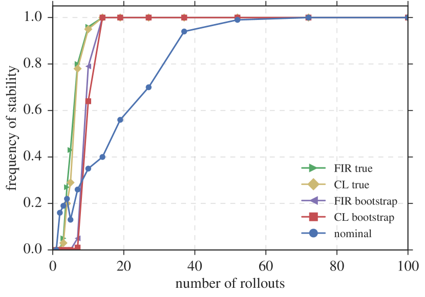
We demonstrate the utility of our method on a simple simulation. In the presented example, we show that simply using the nominal system to design a control policy frequently results in unstable closed-loop behavior, even when there is an abundance of data from the true system. However, the Coarse-ID approach finds a stabilizing controller with few system observations.

1.1 Problem Statement and Our Contributions

The standard optimal control problem aims to find a control sequence that minimizes an expected cost. We assume a dynamical system with state xtnsubscript𝑥𝑡superscript𝑛x_{t}\in\mathbb{R}^{n} can be acted on by a control utpsubscript𝑢𝑡superscript𝑝u_{t}\in\mathbb{R}^{p} and obeys the stochastic dynamics

xt+1=ft(xt,ut,wt)subscript𝑥𝑡1subscript𝑓𝑡subscript𝑥𝑡subscript𝑢𝑡subscript𝑤𝑡\displaystyle x_{t+1}=f_{t}(x_{t},u_{t},w_{t}) (1.1)

where wtsubscript𝑤𝑡w_{t} is a random process with wtsubscript𝑤𝑡w_{t} independent of wtsubscript𝑤superscript𝑡w_{t^{\prime}} for all tt𝑡superscript𝑡t\neq t^{\prime}. Optimal control then seeks to minimize

minimize𝔼[1Tt=1Tct(xt,ut)]subject toxt+1=ft(xt,ut,wt).minimize𝔼delimited-[]1𝑇superscriptsubscript𝑡1𝑇subscript𝑐𝑡subscript𝑥𝑡subscript𝑢𝑡subject tosubscript𝑥𝑡1subscript𝑓𝑡subscript𝑥𝑡subscript𝑢𝑡subscript𝑤𝑡\displaystyle\begin{array}[]{ll}\mbox{minimize}&\mathbb{E}\left[\frac{1}{T}\sum_{t=1}^{T}c_{t}(x_{t},u_{t})\right]\\ \mbox{subject to}&x_{t+1}=f_{t}(x_{t},u_{t},w_{t})\end{array}\,. (1.4)

Here, ctsubscript𝑐𝑡c_{t} denotes the state-control cost at every time step, and the input utsubscript𝑢𝑡u_{t} is allowed to depend on the current state xtsubscript𝑥𝑡x_{t} and all previous states and actions. In this generality, problem (1.4) encapsulates many of the problems considered in the reinforcement learning literature.

The simplest optimal control problem with continuous state is the Linear Quadratic Regulator (LQR), in which costs are a fixed quadratic function of state and control and the dynamics are linear and time-invariant:

minimize𝔼[1Tt=1TxtQxt+ut1Rut1]subject toxt+1=Axt+But+wt.minimize𝔼delimited-[]1𝑇superscriptsubscript𝑡1𝑇superscriptsubscript𝑥𝑡𝑄subscript𝑥𝑡superscriptsubscript𝑢𝑡1𝑅subscript𝑢𝑡1subject tosubscript𝑥𝑡1𝐴subscript𝑥𝑡𝐵subscript𝑢𝑡subscript𝑤𝑡\displaystyle\begin{array}[]{ll}\mbox{minimize}&\mathbb{E}\left[\frac{1}{T}\sum_{t=1}^{T}x_{t}^{*}Qx_{t}+u_{t-1}^{*}Ru_{t-1}\right]\\ \mbox{subject to}&x_{t+1}=Ax_{t}+Bu_{t}+w_{t}\end{array}\,. (1.7)

Here Q𝑄Q (resp. R𝑅R) is a n×n𝑛𝑛n\times n (resp. p×p𝑝𝑝p\times p) positive definite matrix, A𝐴A and B𝐵B are called the state transition matrices, and wtnsubscript𝑤𝑡superscript𝑛w_{t}\in\mathbb{R}^{n} is Gaussian noise with zero-mean and covariance ΣwsubscriptΣ𝑤\Sigma_{w}. Throughout, Msuperscript𝑀M^{*} denotes the Hermitian transpose of the matrix M𝑀M.

In what follows, we will be concerned with the infinite time horizon variant of the LQR problem where we let the time horizon T𝑇T go to infinity and minimize the average cost. When the dynamics are known, this problem has a celebrated closed form solution based on the solution of matrix Riccati equations [64]. Indeed, the optimal solution sets ut=Kxtsubscript𝑢𝑡𝐾subscript𝑥𝑡u_{t}=Kx_{t} for a fixed p×n𝑝𝑛p\times n matrix K𝐾K, and the corresponding optimal cost will serve as our gold-standard baseline to which we will compare the achieved cost of all algorithms.

In the case when the state transition matrices are unknown, fewer results have been established about what cost is achievable. We will assume that we can conduct experiments of the following form: given some initial state x0subscript𝑥0x_{0}, we can evolve the dynamics for T𝑇T time steps using any control sequence {u0,,uT1}subscript𝑢0subscript𝑢𝑇1\{u_{0},\ldots,u_{T-1}\}, measuring the resulting output {x1,,xT}subscript𝑥1subscript𝑥𝑇\{x_{1},\ldots,x_{T}\}. If we run N𝑁N such independent experiments, what infinite time horizon control cost is achievable using only the data collected? For simplicity of bookkeeping, in our analysis we further assume that we can prepare the system in initial state x0=0subscript𝑥00x_{0}=0.

In what follows we will examine the performance of the Coarse-ID control framework in this scenario. We will estimate the errors accrued by least squares estimates (A^,B^)^𝐴^𝐵(\widehat{A},\widehat{B}) of the system dynamics. This estimation error is not easily handled by standard techniques because the design matrix is highly correlated with the model to be estimated. Regardless, for theoretical tractability, we can build a least squares estimate using only the final sample (xT,xT1,uT1)subscript𝑥𝑇subscript𝑥𝑇1subscript𝑢𝑇1(x_{T},x_{T-1},u_{T-1}) of each of the N𝑁N experiments. Indeed, in Section 2 we prove the following

Proposition 1.1.

Define the matrices

GT=[AT1BAT2BB]andFT=[AT1AT2In].formulae-sequencesubscript𝐺𝑇matrixsuperscript𝐴𝑇1𝐵superscript𝐴𝑇2𝐵𝐵andsubscript𝐹𝑇matrixsuperscript𝐴𝑇1superscript𝐴𝑇2subscript𝐼𝑛\displaystyle G_{T}=\begin{bmatrix}A^{T-1}B&A^{T-2}B&\ldots&B\end{bmatrix}\quad\text{and}\quad F_{T}=\begin{bmatrix}A^{T-1}&A^{T-2}&\ldots&I_{n}\end{bmatrix}\>. (1.8)

Assume we collect data from the linear, time-invariant system initialized at x0=0subscript𝑥00x_{0}=0, using inputs ut i.i.d.𝒩(0,σu2Ip)superscriptsimilar-to i.i.d.subscript𝑢𝑡𝒩0superscriptsubscript𝜎𝑢2subscript𝐼𝑝u_{t}~{}\stackrel{{\scriptstyle\mathclap{\text{\scriptsize{ \tiny i.i.d.}}}}}{{\sim}}\mathcal{N}(0,\sigma_{u}^{2}I_{p}) for t=1,,T𝑡1𝑇t=1,...,T. Suppose that the process noise is wt i.i.d.𝒩(0,σw2In)superscriptsimilar-to i.i.d.subscript𝑤𝑡𝒩0superscriptsubscript𝜎𝑤2subscript𝐼𝑛w_{t}~{}\stackrel{{\scriptstyle\mathclap{\text{\scriptsize{ \tiny i.i.d.}}}}}{{\sim}}\mathcal{N}(0,\sigma_{w}^{2}I_{n}) and that

N8(n+p)+16log(4/δ).𝑁8𝑛𝑝164𝛿\displaystyle N\geq 8(n+p)+16\log(4/\delta)\>.

Then, with probability at least 1δ1𝛿1-\delta, the least squares estimator using only the final sample of each trajectory satisfies both the inequality

A^A216σwλmin(σu2GTGT+σw2FTFT)(n+2p)log(36/δ)N,subscriptnorm^𝐴𝐴216subscript𝜎𝑤subscript𝜆superscriptsubscript𝜎𝑢2subscript𝐺𝑇superscriptsubscript𝐺𝑇superscriptsubscript𝜎𝑤2subscript𝐹𝑇superscriptsubscript𝐹𝑇𝑛2𝑝36𝛿𝑁\displaystyle\|\widehat{A}-A\|_{2}\leq\frac{16\sigma_{w}}{\sqrt{\lambda_{\min}(\sigma_{u}^{2}G_{T}G_{T}^{*}+\sigma_{w}^{2}F_{T}F_{T}^{*})}}\sqrt{\frac{(n+2p)\log(36/\delta)}{N}}\>, (1.9)

and the inequality

B^B216σwσu(n+2p)log(36/δ)N.subscriptnorm^𝐵𝐵216subscript𝜎𝑤subscript𝜎𝑢𝑛2𝑝36𝛿𝑁\displaystyle\|\widehat{B}-B\|_{2}\leq\frac{16\sigma_{w}}{\sigma_{u}}\sqrt{\frac{(n+2p)\log(36/\delta)}{N}}\>. (1.10)

The details of the estimation procedure are described in Section 2 below. Note that this estimation result seems to yield an optimal dependence in terms of the number of parameters: (A,B)𝐴𝐵(A,B) together have n(n+p)𝑛𝑛𝑝n(n+p) parameters to learn and each measurement consists of n𝑛n values. Moreover, this proposition further illustrates that not all linear systems are equally easy to estimate. The matrices GTGTsubscript𝐺𝑇superscriptsubscript𝐺𝑇G_{T}G_{T}^{*} and FTFTsubscript𝐹𝑇superscriptsubscript𝐹𝑇F_{T}F_{T}^{*} are finite time controllability Gramians for the control and noise inputs, respectively . These are standard objects in control: each eigenvalue/vector pair of such a Gramian characterizes how much input energy is required to move the system in that particular direction of the state-space. Therefore λmin(σu2GTGT+σw2FTFT)subscript𝜆superscriptsubscript𝜎𝑢2subscript𝐺𝑇superscriptsubscript𝐺𝑇superscriptsubscript𝜎𝑤2subscript𝐹𝑇superscriptsubscript𝐹𝑇\lambda_{\min}\left(\sigma_{u}^{2}G_{T}G_{T}^{*}+\sigma_{w}^{2}F_{T}F_{T}^{*}\right) quantifies the least controllable, and hence most difficult to excite and estimate, mode of the system. This property is captured nicely in our bound, which indicates that for systems for which all modes are easily excitable (i.e., all modes of the system amplify the applied inputs and disturbances), the identification task becomes easier.

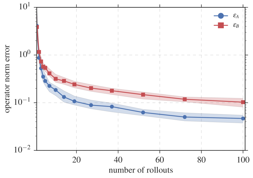
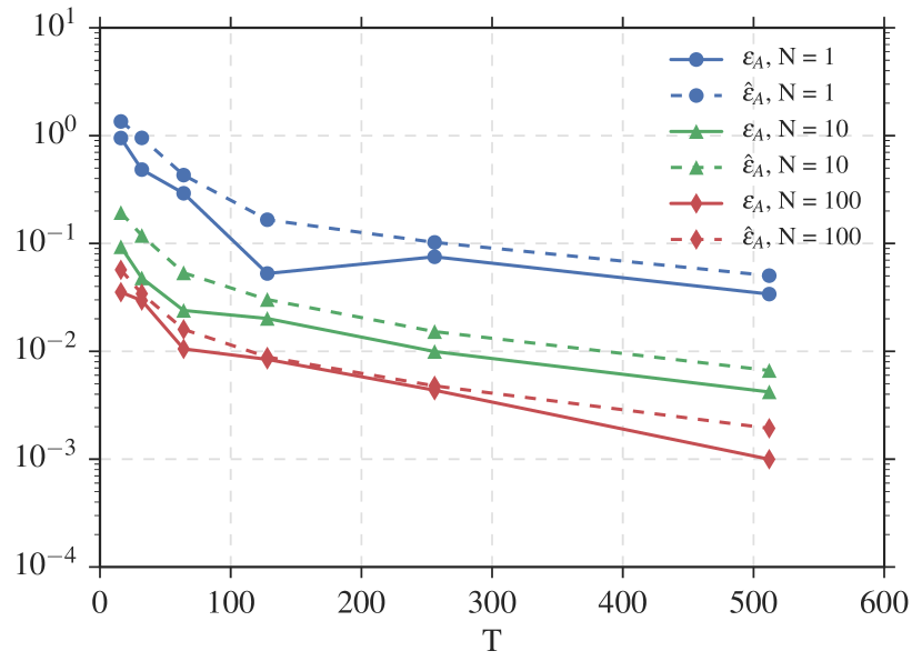
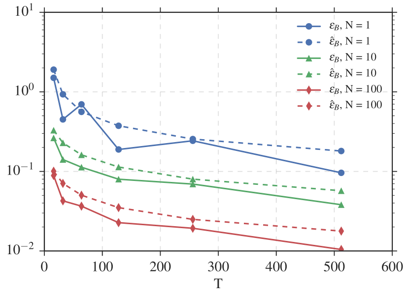
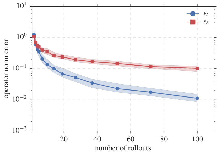
While we cannot compute the operator norm error bounds (1.9) and (1.10) without knowing the true system matrices (A,B)𝐴𝐵(A,B), we present a data-dependent bound in Proposition 2.4. Moreover, as we show in Section 2.3, a simple bootstrap procedure can efficiently upper bound the errors ϵA:=AA^2assignsubscriptitalic-ϵ𝐴subscriptnorm𝐴^𝐴2\epsilon_{A}:=\|A-\widehat{A}\|_{2} and ϵB:=BB^2assignsubscriptitalic-ϵ𝐵subscriptnorm𝐵^𝐵2\epsilon_{B}:=\|B-\widehat{B}\|_{2} from simulation.

With our estimates (A^,B^)^𝐴^𝐵(\widehat{A},\widehat{B}) and error bounds (ϵA,ϵB)subscriptitalic-ϵ𝐴subscriptitalic-ϵ𝐵(\epsilon_{A},\epsilon_{B}) in hand, we can turn to the problem of synthesizing a controller. We can assert with high probability that A=A^+ΔA𝐴^𝐴subscriptΔ𝐴A=\widehat{A}+\Delta_{A}, and B=B^+ΔB𝐵^𝐵subscriptΔ𝐵B=\widehat{B}+\Delta_{B}, for ΔA2ϵAsubscriptnormsubscriptΔ𝐴2subscriptitalic-ϵ𝐴\|\Delta_{A}\|_{2}\leq\epsilon_{A} and ΔB2ϵBsubscriptnormsubscriptΔ𝐵2subscriptitalic-ϵ𝐵\|\Delta_{B}\|_{2}\leq\epsilon_{B}, where the size of the error terms is determined by the number of samples N𝑁N collected. In light of this, it is natural to pose the following robust variant of the standard LQR optimal control problem (1.7), which computes a robustly stabilizing controller that seeks to minimize the worst-case performance of the system given the (high-probability) norm bounds on the perturbations ΔAsubscriptΔ𝐴\Delta_{A} and ΔBsubscriptΔ𝐵\Delta_{B}:

minimizesupΔA2ϵAΔB2ϵBlimT1Tt=1T𝔼[xtQxt+ut1Rut1]subject toxt+1=(A^+ΔA)xt+(B^+ΔB)ut+wt.minimizesubscriptsupremumsubscriptnormsubscriptΔ𝐴2subscriptitalic-ϵ𝐴subscriptnormsubscriptΔ𝐵2subscriptitalic-ϵ𝐵subscript𝑇1𝑇superscriptsubscript𝑡1𝑇𝔼delimited-[]superscriptsubscript𝑥𝑡𝑄subscript𝑥𝑡superscriptsubscript𝑢𝑡1𝑅subscript𝑢𝑡1subject tosubscript𝑥𝑡1^𝐴subscriptΔ𝐴subscript𝑥𝑡^𝐵subscriptΔ𝐵subscript𝑢𝑡subscript𝑤𝑡\begin{array}[]{rl}\mbox{minimize}\>\>\displaystyle\sup\limits_{\begin{subarray}{c}\|\Delta_{A}\|_{2}\leq\epsilon_{A}\\ \|\Delta_{B}\|_{2}\leq\epsilon_{B}\end{subarray}}&\lim_{T\to\infty}\frac{1}{T}\sum_{t=1}^{T}\mathbb{E}\left[x_{t}^{*}Qx_{t}+u_{t-1}^{*}Ru_{t-1}\right]\\ \mbox{subject to}&x_{t+1}=(\hat{A}+\Delta_{A})x_{t}+(\hat{B}+\Delta_{B})u_{t}+w_{t}\end{array}\,. (1.11)

Although classic methods exist for computing such controllers [22, 46, 53, 60], they typically require solving nonconvex optimization problems, and it is not readily obvious how to extract interpretable measures of controller performance as a function of the perturbation sizes ϵAsubscriptitalic-ϵ𝐴\epsilon_{A} and ϵBsubscriptitalic-ϵ𝐵\epsilon_{B}. To that end, we leverage the recently developed System Level Synthesis (SLS) framework [59] to create an alternative robust synthesis procedure. Described in detail in Section 3, SLS lifts the system description into a higher dimensional space that enables efficient search for controllers. At the cost of some conservatism, we are able to guarantee robust stability of the resulting closed-loop system for all admissible perturbations and bound the performance gap between the resulting controller and the optimal LQR controller. This is summarized in the following proposition.

Proposition 1.2.

Let (A^,B^)^𝐴^𝐵(\widehat{A},\widehat{B}) be estimated via the independent data collection scheme used in Proposition 1.1 and 𝐊^^𝐊\mathbf{\widehat{K}} synthesized using robust SLS. Let J^^𝐽\widehat{J} denote the infinite time horizon LQR cost accrued by using the controller 𝐊^^𝐊\mathbf{\widehat{K}} and Jsubscript𝐽J_{\star} denote the optimal LQR cost achieved when (A,B)𝐴𝐵(A,B) are known. Then the relative error in the LQR cost is bounded as

J^JJ𝒪(𝒞LQR(n+p)log(1/δ)N)^𝐽subscript𝐽subscript𝐽𝒪subscript𝒞LQR𝑛𝑝1𝛿𝑁\displaystyle\frac{\widehat{J}-J_{\star}}{J_{\star}}\leq\mathcal{O}\left(\mathcal{C}_{\mathrm{LQR}}\sqrt{\frac{(n+p)\log(1/\delta)}{N}}\right) (1.12)

with probability 1δ1𝛿1-\delta provided N𝑁N is sufficiently large.

The complexity term 𝒞LQRsubscript𝒞LQR\mathcal{C}_{\mathrm{LQR}} depends on the rollout length T𝑇T, the true dynamics, the matrices (Q,R)𝑄𝑅(Q,R) which define the LQR cost, and the variances σu2superscriptsubscript𝜎𝑢2\sigma_{u}^{2} and σw2superscriptsubscript𝜎𝑤2\sigma_{w}^{2} of the control and noise inputs, respectively. The 1δ1𝛿1-\delta probability comes from the probability of estimation error from Proposition 1.1. The particular form of 𝒞LQRsubscript𝒞LQR\mathcal{C}_{\mathrm{LQR}} and concrete requirements on N𝑁N are both provided in Section 4.

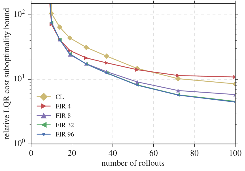
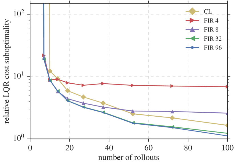
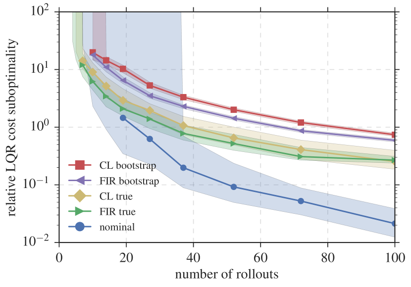
Though the optimization problem formulated by SLS is infinite dimensional, in Section 5 we provide two finite dimensional upper bounds on the optimization that inherit the stability guarantees of the SLS formulation. Moreover, we show via numerical experiments in Section 6 that the controllers synthesized by our optimization do indeed provide stabilizing controllers with small relative error. We further show that settings exist wherein a naïve synthesis procedure that ignores the uncertainty in the state-space parameter estimates produces a controller that performs poorly (or has unstable closed-loop behavior) relative to the controller synthesized using the SLS procedure.

1.2 Related Work

We first describe related work in the estimation of unknown dynamical systems and then turn to connections in the literature on robust control with uncertain models. We will end this review with a discussion of a few works from the reinforcement learning community that have attempted to address the LQR problem and related variants.

Estimation of unknown dynamical systems.

Estimation of unknown systems, especially linear dynamical systems, has a long history in the system identification subfield of control theory. While the text of Ljung [37] covers the classical asymptotic results, our interest is primarily in nonasymptotic results. Early results [11, 57] on nonasymptotic rates for parameter identification featured conservative bounds which are exponential in the system degree and other relevant quantities. More recently, Bento et al. [6] show that when the A𝐴A matrix is stable and induced by a sparse graph, then one can recover the support of A𝐴A from a single trajectory using 1subscript1\ell_{1}-penalized least squares. Furthermore, Hardt et al. [27] provide the first polynomial time guarantee for identifying stable linear systems with outputs. Their guarantees, however, are in terms of predictive output performance of the model, and require an assumption on the true system that is more stringent than stability. It is not clear how their statistical risk guarantee can be used in a downstream robust synthesis procedure.

Next, we turn our attention to system identification of linear systems in the frequency domain. A comprehensive text on these methods (which differ from the aforementioned state-space methods) is the work by Chen and Gu [12]. For stable systems, Helmicki et al. [30] propose to identify a finite impulse response (FIR) approximation by directly estimating the first r𝑟r impulse response coefficients. This method is analyzed in a non-adversarial probabilistic setting by [24, 54], who prove that a polynomial number of samples are sufficient to recover a FIR filter which approximates the true system in both psubscript𝑝\ell_{p}-norm and subscript\mathcal{H}_{\infty}-norm. However, transfer function methods do not easily allow for optimal control with state variables, since they only model the input/output behavior of the system.

In parallel to the system identification community, identification of auto-regressive time series models is a widely studied topic in the statistics literature (see e.g. Box et al. [8] for the classical results). Goldenshluger and Zeevi [25] show that the coefficients of a stationary autoregressive model can be estimated from a single trajectory of length polynomial in 1/(1ρ)11𝜌1/(1-\rho) via least squares, where ρ𝜌\rho denotes the stability radius of the process. They also prove that their rate is minimax optimal. More recently, several authors [34, 40, 43] have studied generalization bounds for non i.i.d. data, extending the standard learning theory guarantees for independent data. At the crux of these arguments lie various mixing assumptions [63], which limits the analysis to only hold for stable dynamical systems. Results in this line of research suggest that systems with smaller mixing time (i.e. systems that are more stable) are easier to identify (i.e. take less samples). Our result in Proposition 1.1, however, suggests instead that identification benefits from more easily excitable systems. While our analysis holds when we have access to full state observations, empirical testing suggests that Proposition 1.1 reflects reality more accurately than arguments based on mixing. In follow up work we have begun to reconcile this issue for stable linear systems [52].

Robust controller design.

For end-to-end guarantees, parameter estimation is only half the picture. Our procedure provides us with a family of system models described by a nominal estimate and a set of unknown but bounded model errors. It is therefore necessary to ensure that the computed controller has stability and performance guarantees for any such admissible realization. The problem of robustly stabilizing such a family of systems is one with a rich history in the controls community. When modelling errors to the nominal system are allowed to be arbitrary norm-bounded linear time-invariant (LTI) operators in feedback with the nominal plant, traditional small-gain theorems and robust synthesis techniques can be applied to exactly solve the problem [14, 64]. However, when the errors are known to have more structure there are more sophisticated techniques based on structured singular values and corresponding μ𝜇\mu-synthesis techniques [16, 20, 45, 62] or integral quadratic constraints (IQCs) [41]. While theoretically appealing and much less conservative than traditional small-gain approaches, the resulting synthesis methods are both computationally intractable (although effective heuristics do exist) and difficult to interpret analytically. In particular, we know of no results in the literature that bound the degradation in performance of controlling an uncertain system in terms of the size of the perturbations affecting it.

To circumvent this issue, we leverage a novel parameterization of robustly stabilizing controllers based on the SLS framework for controller synthesis [59]. We describe this framework in more detail in Section 3. Originally developed to allow for scaling optimal and robust controller synthesis techniques to large-scale systems, the SLS framework can be viewed as a generalization of the celebrated Youla parameterization [61]. We show that SLS allows us to account for model uncertainty in a transparent and analytically tractable way.

PAC learning and reinforcement learning.

Concerning end-to-end guarantees for LQR which couple estimation and control synthesis, our work is most comparable to that of Fiechter [23], who shows that the discounted LQR problem is PAC-learnable. Fietcher analyzes an identify-then-control scheme similar to the one we propose, but there are several key differences. First, our probabilistic bounds on identification are much sharper, by leveraging modern tools from high-dimensional statistics. Second, Fiechter implicitly assumes that the true closed-loop system with the estimated controller is not only stable but also contractive. While this very strong assumption is nearly impossible to verify in practice, contractive closed-loop assumptions are actually pervasive throughout the literature, as we describe below. To the best of our knowledge, our work is the first to properly lift this technical restriction. Third, and most importantly, Fietcher proposes to directly solve the discounted LQR problem with the identified model, and does not take into account any uncertainty in the controller synthesis step. This is problematic for two reasons. First, it is easy to construct an instance of a discounted LQR problem where the optimal solution does not stabilize the true system (see e.g. [47]). Therefore, even in the limit of infinite data, there is no guarantee that the closed-loop system will be stable. Second, even if the optimal solution does stabilize the underlying system, failing to take uncertainty into account can lead to situations where the synthesized controller does not. We will demonstrate this behavior in our experiments.

We are also particularly interested in the LQR problem as a baseline for more complicated problems in reinforcement learning (RL). LQR should be a relatively easy problem in RL because on can learn the dynamics from anywhere in the state space, vastly simplifying the problem of exploration. Hence, it is important to establish how well a pure exploration followed by exploitation strategy can fare on this simple baseline.

There are indeed some related efforts in RL and online learning. Abbasi-Yadkori and Szepesvari [1] propose to use the optimism in the face of uncertainty (OFU) principle for the LQR problem, by maintaining confidence ellipsoids on the true parameter, and using the controller which, in feedback, minimizes the cost objective the most among all systems in the confidence ellipsoid. Ignoring the computational intractability of this approach, their analysis reveals an exponential dependence in the system order in their regret bound, and also makes the very strong assumption that the optimal closed-loop systems are contractive for every A,B𝐴𝐵A,B in the confidence ellipsoid. The regret bound is improved by Ibrahimi et al. [31] to depend linearly on the state dimension under additional sparsity constraints on the dynamics.

In response to the computational intractability of the OFU principle, researchers in RL and online learning have proposed the use of Thompson sampling [49] for exploration. Abeille and Lazaric [2] show that the regret of a Thompson sampling approach for LQR scales as 𝒪~(T2/3)~𝒪superscript𝑇23\widetilde{\mathcal{O}}(T^{2/3}) and improve the result to 𝒪~(T)~𝒪𝑇\widetilde{\mathcal{O}}(\sqrt{T}) in [3], where 𝒪~()~𝒪\widetilde{\mathcal{O}}(\cdot) hides poly-logarithmic factors. However, their results are only valid for the scalar n=d=1𝑛𝑑1n=d=1 setting. Ouyang et al. [44] show that in a Bayesian setting, the expected regret can be bounded by 𝒪~(T)~𝒪𝑇\widetilde{\mathcal{O}}(\sqrt{T}). While this matches the bound of [1], the Bayesian regret is with respect to a particular Gaussian prior distribution over the true model, which differs from the frequentist setting considered in [1, 2, 3]. Furthermore, these works also make the same restrictive assumption that the optimal closed-loop systems are uniformly contractive over some known set.

Jiang et al. [32] propose a general exploration algorithm for contextual decision processes (CDPs) and show that CDPs with low Bellman rank are PAC-learnable; in the LQR setting, they show the Bellman rank is bounded by n2superscript𝑛2n^{2}. While this result is appealing from an information-theoretic standpoint, the proposed algorithm is computationally intractable for continuous problems. Hazan et al. [28, 29] study the problem of prediction in a linear dynamical system via a novel spectral filtering algorithm. Their main result shows that one can compete in a regret setting in terms of prediction error. As mentioned previously, converting prediction error bounds into concrete bounds on sub-optimality of control performance is an open question. Fazel et al. [21] show that randomized search algorithms similar to policy gradient can learn the optimal controller with a polynomial number of samples in the noiseless case; an explicit characterization of the dependence of the sample complexity on the parameters of the true system is not given.

2 System Identification through Least-Squares

To estimate a coarse model of the unknown system dynamics, we turn to the simple and classical method of linear least squares. By running experiments in which the system starts at x0=0subscript𝑥00x_{0}=0 and the dynamics evolve with a given input, we can record the resulting state observations. The set of inputs and outputs from each such experiment will be called a rollout. For system estimation, we excite the system with Gaussian noise for N𝑁N rollouts, each of length T𝑇T. The resulting dataset is {(xt(),ut()):1N,0tT}conditional-setsuperscriptsubscript𝑥𝑡superscriptsubscript𝑢𝑡formulae-sequence1𝑁0𝑡𝑇\{({x}_{t}^{(\ell)},{u}_{t}^{(\ell)})~{}:~{}1\leq\ell\leq N,0\leq t\leq T\}, where t𝑡t indexes the time in one rollout and \ell indexes independent rollouts. Therefore, we can estimate the system dynamics by

(A^,B^)argmin(A,B)=1Nt=0T112Axt()+But()xt+1()22.^𝐴^𝐵subscript𝐴𝐵superscriptsubscript1𝑁superscriptsubscript𝑡0𝑇112superscriptsubscriptnorm𝐴superscriptsubscript𝑥𝑡𝐵superscriptsubscript𝑢𝑡superscriptsubscript𝑥𝑡122\displaystyle(\widehat{A},\widehat{B})\in\arg\min_{(A,B)}\sum_{\ell=1}^{N}\sum_{t=0}^{T-1}\frac{1}{2}\|A{x}_{t}^{(\ell)}+B{u}_{t}^{(\ell)}-{x}_{t+1}^{(\ell)}\|_{2}^{2}. (2.1)

For the Coarse-ID control setting, a good estimate of error is just as important as the estimate of the dynamics. Statistical theory and tools allow us to quantify the error of the least squares estimator. First, we present a theoretical analysis of the error in a simplified setting. Then, we describe a computational bootstrap procedure for error estimation from data alone.

2.1 Least Squares Estimation as a Random Matrix Problem

We begin by explicitly writing the form of the least squares estimator. First, fixing notation to simplify the presentation, let Θ:=[AB](n+p)×nassignΘsuperscriptmatrix𝐴𝐵superscript𝑛𝑝𝑛\Theta:=\begin{bmatrix}A&B\end{bmatrix}^{*}\in\mathbb{R}^{(n+p)\times n} and let zt:=[xtut]n+passignsubscript𝑧𝑡matrixsubscript𝑥𝑡subscript𝑢𝑡superscript𝑛𝑝z_{t}:=\begin{bmatrix}x_{t}\\ u_{t}\end{bmatrix}\in\mathbb{R}^{n+p}. Then the system dynamics can be rewritten, for all t0𝑡0t\geq 0,

xt+1=ztΘ+wt.superscriptsubscript𝑥𝑡1superscriptsubscript𝑧𝑡Θsuperscriptsubscript𝑤𝑡\displaystyle x_{t+1}^{*}=z_{t}^{*}\Theta+w_{t}^{*}\>.

Then in a single rollout, we will collect

X:=[x1x2xT],Z:=[z0z1zT1],W:=[w0w1wT1].formulae-sequenceassign𝑋matrixsuperscriptsubscript𝑥1superscriptsubscript𝑥2superscriptsubscript𝑥𝑇formulae-sequenceassign𝑍matrixsuperscriptsubscript𝑧0superscriptsubscript𝑧1superscriptsubscript𝑧𝑇1assign𝑊matrixsuperscriptsubscript𝑤0superscriptsubscript𝑤1superscriptsubscript𝑤𝑇1\displaystyle X:=\begin{bmatrix}x_{1}^{*}\\ x_{2}^{*}\\ \vdots\\ x_{T}^{*}\end{bmatrix}\>,\>\>Z:=\begin{bmatrix}z_{0}^{*}\\ z_{1}^{*}\\ \vdots\\ z_{T-1}^{*}\end{bmatrix}\>,\>\>W:=\begin{bmatrix}w_{0}^{*}\\ w_{1}^{*}\\ \vdots\\ w_{T-1}^{*}\end{bmatrix}\>. (2.2)

The system dynamics give the identity X=ZΘ+W𝑋𝑍Θ𝑊X=Z\Theta+W. Resetting state of the system to x0=0subscript𝑥00x_{0}=0 each time, we can perform N𝑁N rollouts and collect N𝑁N datasets like (2.2). Having the ability to reset the system to a state independent of past observations will be important for the analysis in the following section, and it is also practically important for potentially unstable systems. Denote the data for each rollout as (X(),Z(),W())superscript𝑋superscript𝑍superscript𝑊(X^{(\ell)},Z^{(\ell)},W^{(\ell)}). With slight abuse of notation, let XNsubscript𝑋𝑁X_{N} be composed of vertically stacked X()superscript𝑋X^{(\ell)}, and similarly for ZNsubscript𝑍𝑁Z_{N} and WNsubscript𝑊𝑁W_{N}. Then we have

XN=ZNΘ+WN.subscript𝑋𝑁subscript𝑍𝑁Θsubscript𝑊𝑁\displaystyle X_{N}=Z_{N}\Theta+W_{N}\>.

The full data least squares estimator for ΘΘ\Theta is (assuming for now invertibility of ZNZNsuperscriptsubscript𝑍𝑁subscript𝑍𝑁Z_{N}^{*}Z_{N}),

Θ^=(ZNZN)1ZNXN=Θ+(ZNZN)1ZNWN.^Θsuperscriptsuperscriptsubscript𝑍𝑁subscript𝑍𝑁1superscriptsubscript𝑍𝑁subscript𝑋𝑁Θsuperscriptsuperscriptsubscript𝑍𝑁subscript𝑍𝑁1superscriptsubscript𝑍𝑁subscript𝑊𝑁\displaystyle\widehat{\Theta}=(Z_{N}^{*}Z_{N})^{-1}Z_{N}^{*}X_{N}=\Theta+(Z_{N}^{*}Z_{N})^{-1}Z_{N}^{*}W_{N}\>. (2.3)

Then the estimation error is given by

E:=Θ^Θ=(ZNZN)1ZNWN.assign𝐸^ΘΘsuperscriptsuperscriptsubscript𝑍𝑁subscript𝑍𝑁1superscriptsubscript𝑍𝑁subscript𝑊𝑁\displaystyle E:=\widehat{\Theta}-\Theta=(Z_{N}^{*}Z_{N})^{-1}Z_{N}^{*}W_{N}\>. (2.4)

The magnitude of this error is the quantity of interest in determining confidence sets around estimates (A^,B^)^𝐴^𝐵(\widehat{A},\widehat{B}). However, since WNsubscript𝑊𝑁W_{N} and ZNsubscript𝑍𝑁Z_{N} are not independent, this estimator is difficult to analyze using standard methods. While this type of analysis is an open problem of interest, in this paper we turn instead to a simplified estimator.

2.2 Theoretical Bounds on Least Squares Error

In this section, we work out the statistical rate for the least squares estimator which uses just the last sample of each trajectory (xT(),xT1(),uT1())superscriptsubscript𝑥𝑇superscriptsubscript𝑥𝑇1superscriptsubscript𝑢𝑇1({x}_{T}^{(\ell)},{x}_{T-1}^{(\ell)},{u}_{T-1}^{(\ell)}). This estimation procedure is made precise in Algorithm 1. Our analysis ideas are analogous to those used to prove statistical rates for standard linear regression, and they leverage recent tools in nonasymptotic analysis of random matrices. The result is presented above in Proposition 1.1.

Algorithm 1 Estimation of linear dynamics with independent data
1:for \ell from 111 to N𝑁N do
2:   x0()=0superscriptsubscript𝑥00{x}_{0}^{(\ell)}=0
3:   for t𝑡t from 00 to T1𝑇1T-1 do
4:      xt+1()=Axt()+But()+wt()superscriptsubscript𝑥𝑡1𝐴superscriptsubscript𝑥𝑡𝐵superscriptsubscript𝑢𝑡superscriptsubscript𝑤𝑡{x}_{t+1}^{(\ell)}=A{x}_{t}^{(\ell)}+B{u}_{t}^{(\ell)}+{w}_{t}^{(\ell)} with wt() i.i.d.𝒩(0,σw2In)superscriptsimilar-to i.i.d.superscriptsubscript𝑤𝑡𝒩0superscriptsubscript𝜎𝑤2subscript𝐼𝑛{w}_{t}^{(\ell)}\stackrel{{\scriptstyle\mathclap{\text{\scriptsize{ \tiny i.i.d.}}}}}{{\sim}}\mathcal{N}(0,\sigma_{w}^{2}I_{n}) and ut() i.i.d.𝒩(0,σu2Ip)superscriptsimilar-to i.i.d.superscriptsubscript𝑢𝑡𝒩0superscriptsubscript𝜎𝑢2subscript𝐼𝑝{u}_{t}^{(\ell)}\stackrel{{\scriptstyle\mathclap{\text{\scriptsize{ \tiny i.i.d.}}}}}{{\sim}}\mathcal{N}(0,\sigma_{u}^{2}I_{p}).
5:   end for
6:end for
7:(A^,B^)argmin(A,B)=1N12AxT1()+BuT1()xT()22^𝐴^𝐵subscript𝐴𝐵superscriptsubscript1𝑁12superscriptsubscriptnorm𝐴superscriptsubscript𝑥𝑇1𝐵superscriptsubscript𝑢𝑇1superscriptsubscript𝑥𝑇22(\widehat{A},\widehat{B})\in\arg\min_{(A,B)}\sum_{\ell=1}^{N}\frac{1}{2}\|A{x}_{T-1}^{(\ell)}+B{u}_{T-1}^{(\ell)}-{x}_{T}^{(\ell)}\|_{2}^{2}

In the context of Proposition 1.1, a single data point from each T𝑇T-step rollout is used. We emphasize that this strategy results in independent data, which can be seen by defining the estimator matrix directly. The previous estimator (2.3) is amended as follows: the matrices defined in (2.2) instead include only the final timestep of each trial, XN=[xT(1)xT(2)xT(N)]subscript𝑋𝑁superscriptmatrixsuperscriptsubscript𝑥𝑇1superscriptsubscript𝑥𝑇2superscriptsubscript𝑥𝑇𝑁X_{N}=\begin{bmatrix}x_{T}^{(1)}&x_{T}^{(2)}&\ldots&x_{T}^{(N)}\end{bmatrix}^{*}, and similar modifications are made to ZNsubscript𝑍𝑁Z_{N} and WNsubscript𝑊𝑁W_{N}. The estimator (2.3) uses these modified matrices, which now contain independent rows. To see this, recall the definition of GTsubscript𝐺𝑇G_{T} and FTsubscript𝐹𝑇F_{T} from (1.8),

GT=[AT1BAT2BB],FT=[AT1AT2In].formulae-sequencesubscript𝐺𝑇matrixsuperscript𝐴𝑇1𝐵superscript𝐴𝑇2𝐵𝐵subscript𝐹𝑇matrixsuperscript𝐴𝑇1superscript𝐴𝑇2subscript𝐼𝑛\displaystyle G_{T}=\begin{bmatrix}A^{T-1}B&A^{T-2}B&...&B\end{bmatrix}\>,\>\>F_{T}=\begin{bmatrix}A^{T-1}&A^{T-2}&...&I_{n}\end{bmatrix}\>.

We can unroll the system dynamics and see that

xT=GT[u0u1uT1]+FT[w0w1wT1].subscript𝑥𝑇subscript𝐺𝑇matrixsubscript𝑢0subscript𝑢1subscript𝑢𝑇1subscript𝐹𝑇matrixsubscript𝑤0subscript𝑤1subscript𝑤𝑇1\displaystyle x_{T}=G_{T}\begin{bmatrix}u_{0}\\ u_{1}\\ \vdots\\ u_{T-1}\end{bmatrix}+F_{T}\begin{bmatrix}w_{0}\\ w_{1}\\ \vdots\\ w_{T-1}\end{bmatrix}\>. (2.5)

Using Gaussian excitation, ut𝒩(0,σu2Ip)similar-tosubscript𝑢𝑡𝒩0subscriptsuperscript𝜎2𝑢subscript𝐼𝑝u_{t}\sim\mathcal{N}(0,\sigma^{2}_{u}I_{p}) gives

[xTuT]𝒩(0,[σu2GTGT+σw2FTFT00σu2Ip]).similar-tomatrixsubscript𝑥𝑇subscript𝑢𝑇𝒩0matrixsubscriptsuperscript𝜎2𝑢subscript𝐺𝑇superscriptsubscript𝐺𝑇subscriptsuperscript𝜎2𝑤subscript𝐹𝑇superscriptsubscript𝐹𝑇00subscriptsuperscript𝜎2𝑢subscript𝐼𝑝\displaystyle\begin{bmatrix}x_{T}\\ u_{T}\end{bmatrix}\sim\mathcal{N}\left(0,\begin{bmatrix}\sigma^{2}_{u}G_{T}G_{T}^{*}+\sigma^{2}_{w}F_{T}F_{T}^{*}&0\\ 0&\sigma^{2}_{u}I_{p}\end{bmatrix}\right)\>. (2.6)

Since FTFT0succeedssubscript𝐹𝑇superscriptsubscript𝐹𝑇0F_{T}F_{T}^{*}\succ 0, as long as both σu,σwsubscript𝜎𝑢subscript𝜎𝑤\sigma_{u},\sigma_{w} are positive, this is a non-degenerate distribution.

Therefore, bounding the estimation error can be achieved via proving a result on the error in random design linear regression with vector valued observations. First, we present a lemma which bounds the spectral norm of the product of two independent Gaussian matrices.

Lemma 2.1.

Fix a δ(0,1)𝛿01\delta\in(0,1) and N2log(1/δ)𝑁21𝛿N\geq 2\log(1/\delta). Let fkmsubscript𝑓𝑘superscript𝑚f_{k}\in\mathbb{R}^{m}, gknsubscript𝑔𝑘superscript𝑛g_{k}\in\mathbb{R}^{n} be independent random vectors fk𝒩(0,Σf)similar-tosubscript𝑓𝑘𝒩0subscriptΣ𝑓f_{k}\sim\mathcal{N}(0,\Sigma_{f}) and gk𝒩(0,Σg)similar-tosubscript𝑔𝑘𝒩0subscriptΣ𝑔g_{k}\sim\mathcal{N}(0,\Sigma_{g}) for 1kN1𝑘𝑁1\leq k\leq N. With probability at least 1δ1𝛿1-\delta,

k=1Nfkgk24Σf21/2Σg21/2N(m+n)log(9/δ).subscriptdelimited-∥∥superscriptsubscript𝑘1𝑁subscript𝑓𝑘superscriptsubscript𝑔𝑘24superscriptsubscriptdelimited-∥∥subscriptΣ𝑓212superscriptsubscriptdelimited-∥∥subscriptΣ𝑔212𝑁𝑚𝑛9𝛿\displaystyle\left\lVert\sum_{k=1}^{N}f_{k}g_{k}^{*}\right\rVert_{2}\leq 4\lVert\Sigma_{f}\rVert_{2}^{1/2}\lVert\Sigma_{g}\rVert_{2}^{1/2}\sqrt{N(m+n)\log(9/\delta)}\>.

We believe this bound to be standard, and include a proof in the appendix for completeness. Lemma 2.1 shows that if X𝑋X is n1×Nsubscript𝑛1𝑁n_{1}\times N with i.i.d. 𝒩(0,1)𝒩01\mathcal{N}(0,1) entries and Y𝑌Y is N×n2𝑁subscript𝑛2N\times n_{2} with i.i.d. 𝒩(0,1)𝒩01\mathcal{N}(0,1) entries, and X𝑋X and Y𝑌Y are independent, then with probability at least 1δ1𝛿1-\delta we have

XY24N(n1+n2)log(9/δ).subscriptdelimited-∥∥𝑋𝑌24𝑁subscript𝑛1subscript𝑛29𝛿\displaystyle\lVert XY\rVert_{2}\leq 4\sqrt{N(n_{1}+n_{2})\log(9/\delta)}\>.

Next, we state a standard nonasymptotic bound on the minimum singular value of a standard Wishart matrix (see e.g. Corollary 5.35 of [56]).

Lemma 2.2.

Let XN×n𝑋superscript𝑁𝑛X\in\mathbb{R}^{N\times n} have i.i.d. 𝒩(0,1)𝒩01\mathcal{N}(0,1) entries. With probability at least 1δ1𝛿1-\delta,

λmin(XX)Nn2log(1/δ).subscript𝜆superscript𝑋𝑋𝑁𝑛21𝛿\displaystyle\sqrt{\lambda_{\min}(X^{*}X)}\geq\sqrt{N}-\sqrt{n}-\sqrt{2\log(1/\delta)}\>.

We combine the previous lemmas into a statement on the error of random design regression.

Lemma 2.3.

Let z1,,zNnsubscript𝑧1subscript𝑧𝑁superscript𝑛z_{1},...,z_{N}\in\mathbb{R}^{n} be i.i.d. from 𝒩(0,Σ)𝒩0Σ\mathcal{N}(0,\Sigma) with ΣΣ\Sigma invertible. Let Z:=[z1zN]assignsuperscript𝑍matrixsubscript𝑧1subscript𝑧𝑁Z^{*}:=\begin{bmatrix}z_{1}&...&z_{N}\end{bmatrix}. Let WN×p𝑊superscript𝑁𝑝W\in\mathbb{R}^{N\times p} with each entry i.i.d. 𝒩(0,σw2)𝒩0superscriptsubscript𝜎𝑤2\mathcal{N}(0,\sigma_{w}^{2}) and independent of Z𝑍Z. Let E:=(ZZ)ZWassign𝐸superscriptsuperscript𝑍𝑍superscript𝑍𝑊E:=(Z^{*}Z)^{{\dagger}}Z^{*}W, and suppose that

N8n+16log(2/δ).𝑁8𝑛162𝛿\displaystyle N\geq 8n+16\log(2/\delta)\>. (2.7)

For any fixed matrix Q𝑄Q, we have with probability at least 1δ1𝛿1-\delta,

QE216σwQΣ1/22(n+p)log(18/δ)N.subscriptdelimited-∥∥𝑄𝐸216subscript𝜎𝑤subscriptdelimited-∥∥𝑄superscriptΣ122𝑛𝑝18𝛿𝑁\displaystyle\lVert QE\rVert_{2}\leq 16\sigma_{w}\lVert Q\Sigma^{-1/2}\rVert_{2}\sqrt{\frac{(n+p)\log(18/\delta)}{N}}\>.
Proof.

First, observe that Z𝑍Z is equal in distribution to XΣ1/2𝑋superscriptΣ12X\Sigma^{1/2}, where XN×n𝑋superscript𝑁𝑛X\in\mathbb{R}^{N\times n} has i.i.d. 𝒩(0,1)𝒩01\mathcal{N}(0,1) entries. By Lemma 2.2, with probability at least 1δ/21𝛿21-\delta/2,

λmin(XX)Nn2log(2/δ)N/2.subscript𝜆superscript𝑋𝑋𝑁𝑛22𝛿𝑁2\displaystyle\sqrt{\lambda_{\min}(X^{*}X)}\geq\sqrt{N}-\sqrt{n}-\sqrt{2\log(2/\delta)}\geq\sqrt{N}/2\>.

The last inequality uses (2.7) combined with the inequality (a+b)22(a2+b2)superscript𝑎𝑏22superscript𝑎2superscript𝑏2(a+b)^{2}\leq 2(a^{2}+b^{2}). Furthermore, by Lemma 2.1 and (2.7), with probability at least 1δ/21𝛿21-\delta/2,

XW24σwN(n+p)log(18/δ).subscriptdelimited-∥∥superscript𝑋𝑊24subscript𝜎𝑤𝑁𝑛𝑝18𝛿\displaystyle\lVert X^{*}W\rVert_{2}\leq 4\sigma_{w}\sqrt{N(n+p)\log(18/\delta)}\>.

Let \mathcal{E} denote the event which is the intersection of the two previous events. By a union bound, ()1δ1𝛿\mathbb{P}(\mathcal{E})\geq 1-\delta. We continue the rest of the proof assuming the event \mathcal{E} holds. Since XXsuperscript𝑋𝑋X^{*}X is invertible,

QE=Q(ZZ)ZW=Q(Σ1/2XXΣ1/2)Σ1/2XW=QΣ1/2(XX)1XW.𝑄𝐸𝑄superscriptsuperscript𝑍𝑍superscript𝑍𝑊𝑄superscriptsuperscriptΣ12superscript𝑋𝑋superscriptΣ12superscriptΣ12superscript𝑋𝑊𝑄superscriptΣ12superscriptsuperscript𝑋𝑋1superscript𝑋𝑊\displaystyle QE=Q(Z^{*}Z)^{{\dagger}}Z^{*}W=Q(\Sigma^{1/2}X^{*}X\Sigma^{1/2})^{{\dagger}}\Sigma^{1/2}X^{*}W=Q\Sigma^{-1/2}(X^{*}X)^{-1}X^{*}W\>.

Taking operator norms on both sides,

QE2QΣ1/22(XX)12XW2=QΣ1/22XW2λmin(XX).subscriptdelimited-∥∥𝑄𝐸2subscriptdelimited-∥∥𝑄superscriptΣ122subscriptdelimited-∥∥superscriptsuperscript𝑋𝑋12subscriptdelimited-∥∥superscript𝑋𝑊2subscriptdelimited-∥∥𝑄superscriptΣ122subscriptdelimited-∥∥superscript𝑋𝑊2subscript𝜆superscript𝑋𝑋\displaystyle\lVert QE\rVert_{2}\leq\lVert Q\Sigma^{-1/2}\rVert_{2}\lVert(X^{*}X)^{-1}\rVert_{2}\lVert X^{*}W\rVert_{2}=\lVert Q\Sigma^{-1/2}\rVert_{2}\frac{\lVert X^{*}W\rVert_{2}}{\lambda_{\min}(X^{*}X)}\>.

Combining the inequalities above,

XW2λmin(XX)16σw(n+p)log(18/δ)N.subscriptdelimited-∥∥superscript𝑋𝑊2subscript𝜆superscript𝑋𝑋16subscript𝜎𝑤𝑛𝑝18𝛿𝑁\displaystyle\frac{\lVert X^{*}W\rVert_{2}}{\lambda_{\min}(X^{*}X)}\leq 16\sigma_{w}\sqrt{\frac{(n+p)\log(18/\delta)}{N}}\>.

The result now follows. ∎

Using this result on random design linear regression, we are now ready to analyze the estimation errors of the identification in Algorithm 1 and provide a proof of Proposition 1.1.

Proof.

Consider the least squares estimation error (2.4) with modified single-sample-per-rollout matrices. Recall that rows of the design matrix ZNsubscript𝑍𝑁Z_{N} are distributed as independent normals, as in (2.6). Then applying Lemma 2.3 with QA=[In0]subscript𝑄𝐴matrixsubscript𝐼𝑛0Q_{A}=\begin{bmatrix}I_{n}&0\end{bmatrix} so that QAEsubscript𝑄𝐴𝐸Q_{A}E extracts only the estimate for A𝐴A, we conclude that with probability at least 1δ/21𝛿21-\delta/2,

A^A216σwλmin(σu2GTGT+σw2FTFT)(n+2p)log(36/δ)N,subscriptdelimited-∥∥^𝐴𝐴216subscript𝜎𝑤subscript𝜆superscriptsubscript𝜎𝑢2subscript𝐺𝑇superscriptsubscript𝐺𝑇superscriptsubscript𝜎𝑤2subscript𝐹𝑇superscriptsubscript𝐹𝑇𝑛2𝑝36𝛿𝑁\displaystyle\lVert\widehat{A}-A\rVert_{2}\leq\frac{16\sigma_{w}}{\sqrt{\lambda_{\min}(\sigma_{u}^{2}G_{T}G_{T}^{*}+\sigma_{w}^{2}F_{T}F_{T}^{*})}}\sqrt{\frac{(n+2p)\log(36/\delta)}{N}}\>, (2.8)

as long as N8(n+p)+16log(4/δ)𝑁8𝑛𝑝164𝛿N\geq 8(n+p)+16\log(4/\delta). Now applying Lemma 2.3 under the same condition on N𝑁N with QB=[0Ip]subscript𝑄𝐵matrix0subscript𝐼𝑝Q_{B}=\begin{bmatrix}0&I_{p}\end{bmatrix}, we have with probability at least 1δ/21𝛿21-\delta/2,

B^B216σwσu(n+2p)log(36/δ)N.subscriptdelimited-∥∥^𝐵𝐵216subscript𝜎𝑤subscript𝜎𝑢𝑛2𝑝36𝛿𝑁\displaystyle\lVert\widehat{B}-B\rVert_{2}\leq\frac{16\sigma_{w}}{\sigma_{u}}\sqrt{\frac{(n+2p)\log(36/\delta)}{N}}\>. (2.9)

The result follows by application of the union bound. ∎

There are several interesting points to make about the guarantees offered by Proposition 1.1. First, as mentioned in the introduction, there are n(n+p)𝑛𝑛𝑝n(n+p) parameters to learn and our bound states that we need O(n+p)𝑂𝑛𝑝O(n+p) measurements, each measurement providing n𝑛n values. Hence, this appears to be an optimal dependence with respect to the parameters n𝑛n and p𝑝p. Second, note that intuitively, if the system amplifies the control and noise inputs in all directions of the state-space, as captured by the minimum eigenvalues of the control and disturbance Gramians GTGTsubscript𝐺𝑇superscriptsubscript𝐺𝑇G_{T}G_{T}^{*} or FTFTsubscript𝐹𝑇superscriptsubscript𝐹𝑇F_{T}F_{T}^{*}, respectively, then the system has a larger “signal-to-noise” ratio and the system matrix A𝐴A is easier to estimate. On the other hand, this measure of the excitability of the system has no impact on learning B𝐵B. Unlike in Fiechter’s work [23], we do not need to assume that GTGTsubscript𝐺𝑇superscriptsubscript𝐺𝑇G_{T}G_{T}^{*} is invertible. As long as the process noise is not degenerate, it will excite all modes of the system.

Finally, we note that the Proposition 1.1 offers a data independent guarantee for the estimation of the parameters (A,B)𝐴𝐵(A,B). We can also provide data dependent guarantees, which will be less conservative in practice. The next result shows how we can use the observed states and inputs to obtain more refined confidence sets than the ones offered by Proposition 1.1. The proof is deferred to Appendix B.

Proposition 2.4.

Assume we have N𝑁N independent samples (y(),x(),u())superscript𝑦superscript𝑥superscript𝑢(y^{(\ell)},x^{(\ell)},u^{(\ell)}) such that

y()=Ax()+Bu()+w(),superscript𝑦𝐴superscript𝑥𝐵superscript𝑢superscript𝑤\displaystyle y^{(\ell)}=Ax^{(\ell)}+Bu^{(\ell)}+w^{(\ell)},

where w()superscript𝑤w^{(\ell)} are i.i.d. 𝒩(0,σw2In)𝒩0superscriptsubscript𝜎𝑤2subscript𝐼𝑛\mathcal{N}(0,\sigma_{w}^{2}I_{n}) and are independent from x()superscript𝑥x^{(\ell)} and u()superscript𝑢u^{(\ell)}. Also, let us assume that Nn+p𝑁𝑛𝑝N\geq n+p. Then, with probability 1δ1𝛿1-\delta, we have

[(A^A)(B^B)][(A^A)(B^B)]C(n,p,δ)(=1N[x()u()][(x())(u())])1,precedes-or-equalsmatrixsuperscript^𝐴𝐴topsuperscript^𝐵𝐵topmatrix^𝐴𝐴^𝐵𝐵𝐶𝑛𝑝𝛿superscriptsuperscriptsubscript1𝑁matrixsuperscript𝑥superscript𝑢matrixsuperscriptsuperscript𝑥topsuperscriptsuperscript𝑢top1\displaystyle\begin{bmatrix}(\widehat{A}-A)^{\top}\\ (\widehat{B}-B)^{\top}\end{bmatrix}\begin{bmatrix}(\widehat{A}-A)&(\widehat{B}-B)\end{bmatrix}\preceq C(n,p,\delta)\left(\sum_{\ell=1}^{N}\begin{bmatrix}x^{(\ell)}\\ u^{(\ell)}\end{bmatrix}\begin{bmatrix}(x^{(\ell)})^{\top}&(u^{(\ell)})^{\top}\end{bmatrix}\right)^{-1},

where C(n,p,δ)=σw2(n+p+n+2log(1/δ))2𝐶𝑛𝑝𝛿superscriptsubscript𝜎𝑤2superscript𝑛𝑝𝑛21𝛿2C(n,p,\delta)=\sigma_{w}^{2}(\sqrt{n+p}+\sqrt{n}+\sqrt{2\log(1/\delta)})^{2}. If the matrix on the right hand side has zero as an eigenvalue, we define the inverse of that eigenvalue to be infinity.

Proposition 2.4 is a general result that does not require the inputs u()superscript𝑢u^{(\ell)} to be normally distributed and it allows the states x()superscript𝑥x^{(\ell)} to be arbitrary as long as all the samples (y(),x(),u())superscript𝑦superscript𝑥superscript𝑢(y^{(\ell)},x^{(\ell)},u^{(\ell)}) are independent and the process noise w()superscript𝑤w^{(\ell)} is normally distributed. Nonetheless, both Propositions 1.1 and 2.4 require estimating (A,B)𝐴𝐵(A,B) from independent samples. In practice, one would collect rollouts from the system, which consist of many dependent measurements. In that case, using all the data is preferable. Since the guarantees offered in this section do not apply in that case, in the next section we study a different procedure for estimating the size of the estimation error.

2.3 Estimating Model Uncertainty with the Bootstrap

In the previous sections we offered theoretical guarantees on the performance of the least squares estimation of A𝐴A and B𝐵B from independent samples. However, there are two important limitations to using such guarantees in practice to offer upper bounds on ϵA=AA^2subscriptitalic-ϵ𝐴subscriptdelimited-∥∥𝐴^𝐴2\epsilon_{A}=\lVert A-\widehat{A}\rVert_{2} and ϵB=BB^2subscriptitalic-ϵ𝐵subscriptdelimited-∥∥𝐵^𝐵2\epsilon_{B}=\lVert B-\widehat{B}\rVert_{2}. First, using only one sample per system rollout is empirically less efficient than using all available data for estimation. Second, even optimal statistical analyses often do not recover constant factors that match practice. For purposes of robust control, it is important to obtain upper bounds on ϵAsubscriptitalic-ϵ𝐴\epsilon_{A} and ϵBsubscriptitalic-ϵ𝐵\epsilon_{B} that are not too conservative. Thus, we aim to find ϵ^Asubscript^italic-ϵ𝐴\widehat{\epsilon}_{A} and ϵ^Bsubscript^italic-ϵ𝐵\widehat{\epsilon}_{B} such that ϵAϵ^Asubscriptitalic-ϵ𝐴subscript^italic-ϵ𝐴\epsilon_{A}\leq\widehat{\epsilon}_{A} and ϵBϵ^Bsubscriptitalic-ϵ𝐵subscript^italic-ϵ𝐵\epsilon_{B}\leq\widehat{\epsilon}_{B} with high probability.

We propose a vanilla bootstrap method for estimating ϵ^Asubscript^italic-ϵ𝐴\widehat{\epsilon}_{A} and ϵ^Bsubscript^italic-ϵ𝐵\widehat{\epsilon}_{B}. Bootstrap methods have had a profound impact in both theoretical and applied statistics since their introduction [19]. These methods are used to estimate statistical quantities (e.g. confidence intervals) by sampling synthetic data from an empirical distribution determined by the available data. For the problem at hand we propose the procedure described in Algorithm 2.111We assume that σusubscript𝜎𝑢\sigma_{u} and σwsubscript𝜎𝑤\sigma_{w} are known. Otherwise they can be estimated from data.

Algorithm 2 Bootstrap estimation of ϵAsubscriptitalic-ϵ𝐴\epsilon_{A} and ϵBsubscriptitalic-ϵ𝐵\epsilon_{B}
1:Input: confidence parameter δ𝛿\delta, number of trials M𝑀M, data {(xt(i),ut(i))}1iN1tTsubscriptsuperscriptsubscript𝑥𝑡𝑖superscriptsubscript𝑢𝑡𝑖1𝑖𝑁1𝑡𝑇\{({x}_{t}^{(i)},{u}_{t}^{(i)})\}_{\begin{subarray}{c}1\leq i\leq N\\ 1\leq t\leq T\end{subarray}}, and (A^,B^)^𝐴^𝐵(\widehat{A},\widehat{B}) a minimizer of =1Nt=0T112Axt()+But()xt+1()22.superscriptsubscript1𝑁superscriptsubscript𝑡0𝑇112superscriptsubscriptdelimited-∥∥𝐴superscriptsubscript𝑥𝑡𝐵superscriptsubscript𝑢𝑡superscriptsubscript𝑥𝑡122\sum_{\ell=1}^{N}\sum_{t=0}^{T-1}\frac{1}{2}\lVert A{x}_{t}^{(\ell)}+B{u}_{t}^{(\ell)}-{x}_{t+1}^{(\ell)}\rVert_{2}^{2}.
2:for M𝑀M trials do
3:   for \ell from 111 to N𝑁N do
4:      x^0()=x0()superscriptsubscript^𝑥0superscriptsubscript𝑥0\widehat{{x}}_{0}^{(\ell)}={x}_{0}^{(\ell)}
5:      for t𝑡t from 00 to T1𝑇1T-1 do
6:         x^t+1()=A^x^t()+B^u^t()+w^t()superscriptsubscript^𝑥𝑡1^𝐴superscriptsubscript^𝑥𝑡^𝐵superscriptsubscript^𝑢𝑡superscriptsubscript^𝑤𝑡\widehat{{x}}_{t+1}^{(\ell)}=\widehat{A}\widehat{{x}}_{t}^{(\ell)}+\widehat{B}\widehat{{u}}_{t}^{(\ell)}+\widehat{{w}}_{t}^{(\ell)} with w^t() i.i.d.𝒩(0,σw2In)superscriptsimilar-to i.i.d.superscriptsubscript^𝑤𝑡𝒩0superscriptsubscript𝜎𝑤2subscript𝐼𝑛\widehat{{w}}_{t}^{(\ell)}\stackrel{{\scriptstyle\mathclap{\text{\scriptsize{ \tiny i.i.d.}}}}}{{\sim}}\mathcal{N}(0,\sigma_{w}^{2}I_{n}) and u^t() i.i.d.𝒩(0,σu2Ip)superscriptsimilar-to i.i.d.superscriptsubscript^𝑢𝑡𝒩0superscriptsubscript𝜎𝑢2subscript𝐼𝑝\widehat{{u}}_{t}^{(\ell)}\stackrel{{\scriptstyle\mathclap{\text{\scriptsize{ \tiny i.i.d.}}}}}{{\sim}}\mathcal{N}(0,\sigma_{u}^{2}I_{p}).
7:      end for
8:   end for
9:   (A~,B~)argmin(A,B)=1Nt=0T112Ax^t()+Bu^t()x^t+1()22~𝐴~𝐵subscript𝐴𝐵superscriptsubscript1𝑁superscriptsubscript𝑡0𝑇112superscriptsubscriptnorm𝐴superscriptsubscript^𝑥𝑡𝐵superscriptsubscript^𝑢𝑡superscriptsubscript^𝑥𝑡122(\widetilde{A},\widetilde{B})\in\arg\min_{(A,B)}\sum_{\ell=1}^{N}\sum_{t=0}^{T-1}\frac{1}{2}\|A\widehat{{x}}_{t}^{(\ell)}+B\widehat{{u}}_{t}^{(\ell)}-\widehat{{x}}_{t+1}^{(\ell)}\|_{2}^{2}.
10:   record ϵ~A=A^A~2subscript~italic-ϵ𝐴subscriptnorm^𝐴~𝐴2\widetilde{\epsilon}_{A}=\|\widehat{A}-\widetilde{A}\|_{2} and ϵ~B=B^B~2subscript~italic-ϵ𝐵subscriptnorm^𝐵~𝐵2\widetilde{\epsilon}_{B}=\|\widehat{B}-\widetilde{B}\|_{2}.
11:end for
12:Output: ϵ^Asubscript^italic-ϵ𝐴\widehat{\epsilon}_{A} and ϵ^Bsubscript^italic-ϵ𝐵\widehat{\epsilon}_{B}, the 100(1δ)1001𝛿100(1-\delta)th percentiles of the ϵ~Asubscript~italic-ϵ𝐴\widetilde{\epsilon}_{A}’s and the ϵ~Bsubscript~italic-ϵ𝐵\widetilde{\epsilon}_{B}’s.

For ϵ^Asubscript^italic-ϵ𝐴\widehat{\epsilon}_{A} and ϵ^Bsubscript^italic-ϵ𝐵\widehat{\epsilon}_{B} estimated by Algorithm 2 we intuitively have

(AA^2ϵ^A)1δand(BB^2ϵ^B)1δ.formulae-sequencesubscriptdelimited-∥∥𝐴^𝐴2subscript^italic-ϵ𝐴1𝛿andsubscriptdelimited-∥∥𝐵^𝐵2subscript^italic-ϵ𝐵1𝛿\displaystyle\mathbb{P}(\lVert A-\widehat{A}\rVert_{2}\leq\widehat{\epsilon}_{A})\approx 1-\delta\quad\text{and}\quad\mathbb{P}(\lVert B-\widehat{B}\rVert_{2}\leq\widehat{\epsilon}_{B})\approx 1-\delta.

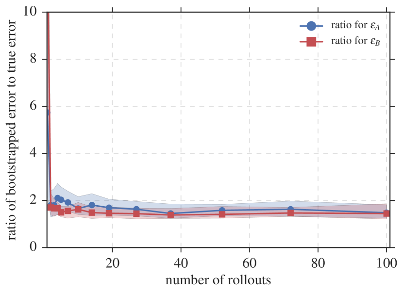
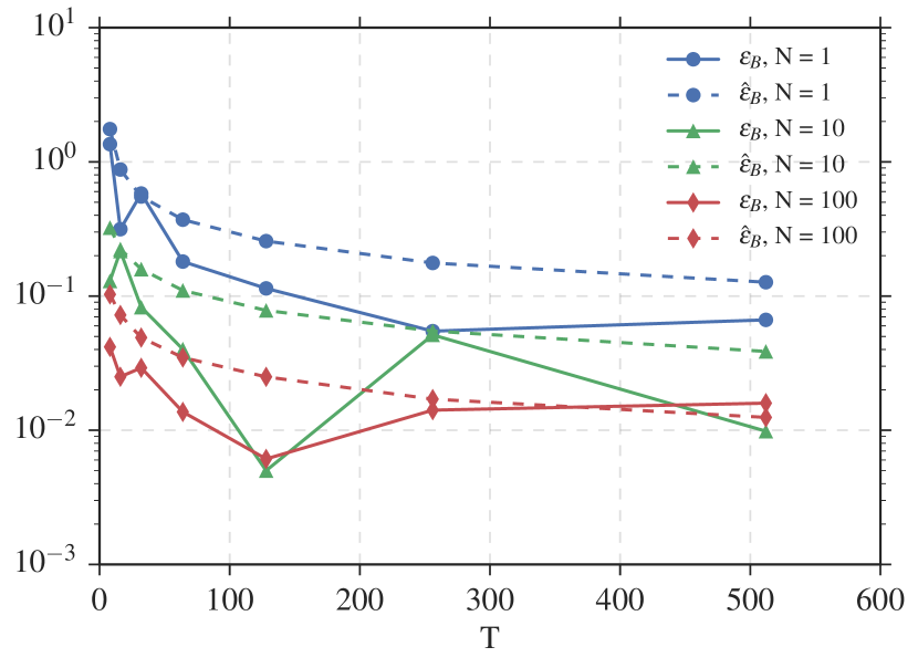
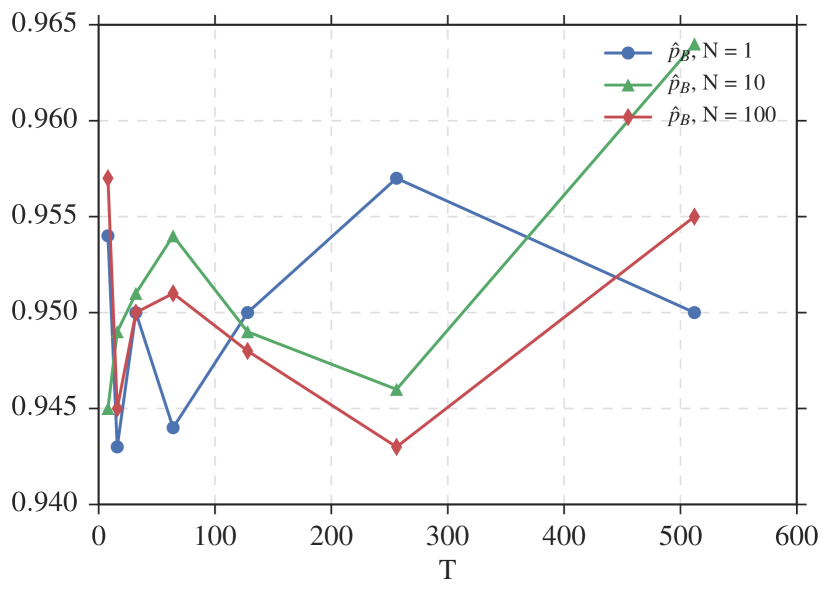
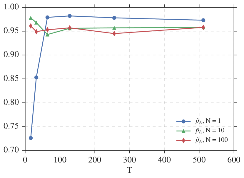
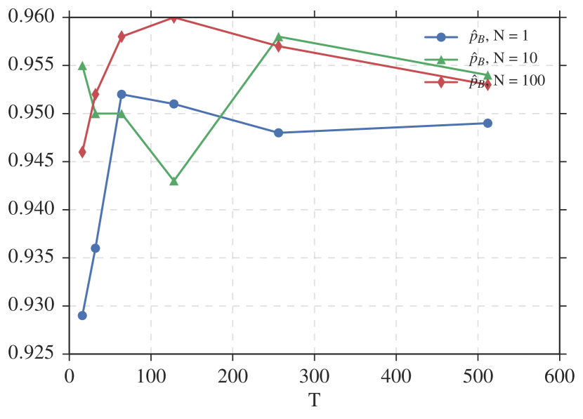
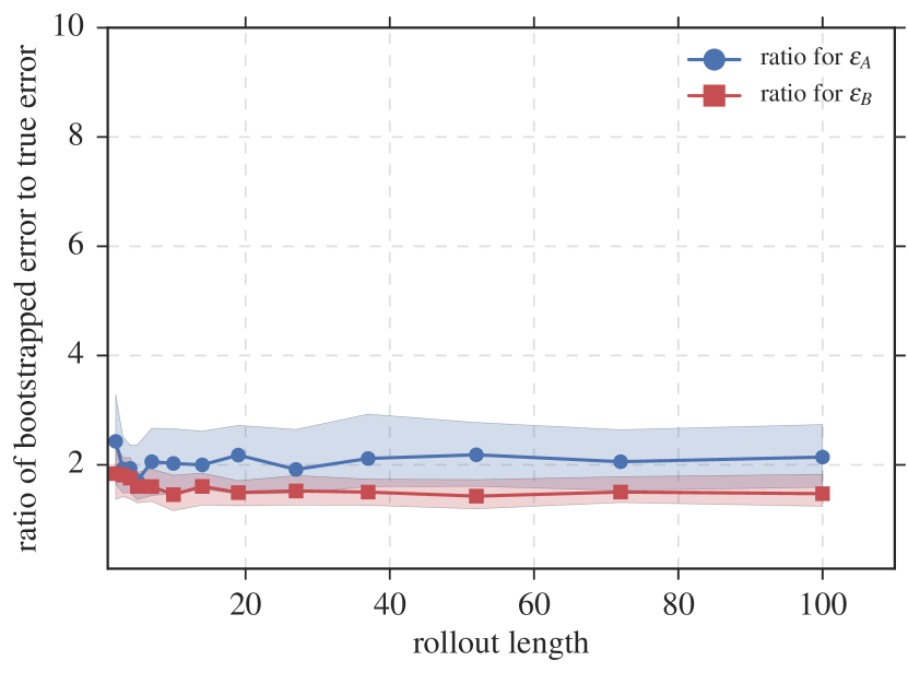
There are many known guarantees for the bootstrap, particularly for the parametric version we use. We do not discuss these results here; for more details see texts by Van Der Vaart and Wellner [55], Shao and Tu [50], and Hall [26]. Instead, in Appendix F we show empirically the performance of the bootstrap for our estimation problem. For mission critical systems, where empirical validation is insufficient, the statistical error bounds presented in Section 2.2 give guarantees on the size of ϵAsubscriptitalic-ϵ𝐴\epsilon_{A}, ϵBsubscriptitalic-ϵ𝐵\epsilon_{B}. In general, data dependent error guarantees will be less conservative. In follow up work we offer guarantees similar to the ones presented in Section 2.2 for estimation of linear dynamics from dependent data [52].

3 Robust Synthesis

With estimates of the system (A^,B^)^𝐴^𝐵(\widehat{A},\widehat{B}) and operator norm error bounds (ϵA,ϵB)subscriptitalic-ϵ𝐴subscriptitalic-ϵ𝐵(\epsilon_{A},\epsilon_{B}) in hand, we now turn to control design. In this section we introduce some useful tools from System Level Synthesis (SLS), a recently developed approach to control design that relies on a particular parameterization of signals in a control system [39, 59]. We review the main SLS framework, highlighting the key constructions that we will use to solve the robust LQR problem. As we show in this and the following section, using the SLS framework, as opposed to traditional techniques from robust control, allows us to (a) compute robust controllers using semidefinite programming, and (b) provide sub-optimality guarantees in terms of the size of the uncertainties on our system estimates.

3.1 Useful Results from System Level Synthesis

The SLS framework focuses on the system responses of a closed-loop system. As a motivating example, consider linear dynamics under a fixed a static state-feedback control policy K𝐾K, i.e., let uk=Kxksubscript𝑢𝑘𝐾subscript𝑥𝑘u_{k}=Kx_{k}. Then, the closed loop map from the disturbance process {w0,w1,}subscript𝑤0subscript𝑤1\{w_{0},w_{1},\dots\} to the state xksubscript𝑥𝑘x_{k} and control input uksubscript𝑢𝑘u_{k} at time k𝑘k is given by

xk=t=1k(A+BK)ktwt1,uk=t=1kK(A+BK)ktwt1.subscript𝑥𝑘superscriptsubscript𝑡1𝑘superscript𝐴𝐵𝐾𝑘𝑡subscript𝑤𝑡1subscript𝑢𝑘superscriptsubscript𝑡1𝑘𝐾superscript𝐴𝐵𝐾𝑘𝑡subscript𝑤𝑡1\begin{array}[]{rcl}x_{k}&=&\sum_{t=1}^{k}(A+BK)^{k-t}w_{t-1}\>,\\ u_{k}&=&\sum_{t=1}^{k}K(A+BK)^{k-t}w_{t-1}\>.\end{array} (3.1)

Letting Φx(k):=(A+BK)k1assignsubscriptΦ𝑥𝑘superscript𝐴𝐵𝐾𝑘1\Phi_{x}(k):=(A+BK)^{k-1} and Φu(k):=K(A+BK)k1assignsubscriptΦ𝑢𝑘𝐾superscript𝐴𝐵𝐾𝑘1\Phi_{u}(k):=K(A+BK)^{k-1}, we can rewrite Eq. (3.1) as

[xkuk]=t=1k[Φx(kt+1)Φu(kt+1)]wt1,matrixsubscript𝑥𝑘subscript𝑢𝑘superscriptsubscript𝑡1𝑘matrixsubscriptΦ𝑥𝑘𝑡1subscriptΦ𝑢𝑘𝑡1subscript𝑤𝑡1\begin{bmatrix}x_{k}\\ u_{k}\end{bmatrix}=\sum_{t=1}^{k}\begin{bmatrix}\Phi_{x}(k-t+1)\\ \Phi_{u}(k-t+1)\end{bmatrix}w_{t-1}\>, (3.2)

where {Φx(k),Φu(k)}subscriptΦ𝑥𝑘subscriptΦ𝑢𝑘\{\Phi_{x}(k),\Phi_{u}(k)\} are called the closed-loop system response elements induced by the static controller K𝐾K.

Note that even when the control is a linear function of the state and its past history (i.e. a linear dynamic controller), the expression (3.2) is valid. Though we conventionally think of the control policy as a function mapping states to input, whenever such a mapping is linear, both the control input and the state can be written as linear functions of the disturbance signal wtsubscript𝑤𝑡w_{t}. With such an identification, the dynamics require that the {Φx(k),Φu(k)}subscriptΦ𝑥𝑘subscriptΦ𝑢𝑘\{\Phi_{x}(k),\Phi_{u}(k)\} must obey the constraints

Φx(k+1)=AΦx(k)+BΦu(k),Φx(1)=I,k1,formulae-sequencesubscriptΦ𝑥𝑘1𝐴subscriptΦ𝑥𝑘𝐵subscriptΦ𝑢𝑘formulae-sequencesubscriptΦ𝑥1𝐼for-all𝑘1\Phi_{x}(k+1)=A\Phi_{x}(k)+B\Phi_{u}(k)\>,\>\>\Phi_{x}(1)=I\>,\>\>\forall k\geq 1\>, (3.3)

As we describe in more detail below in Theorem 3.1, these constraints are in fact both necessary and sufficient. Working with closed-loop system responses allows us to cast optimal control problems as optimization problems over elements {Φx(k),Φu(k)}subscriptΦ𝑥𝑘subscriptΦ𝑢𝑘\{\Phi_{x}(k),\Phi_{u}(k)\}, constrained to satisfy the affine equations (3.3). Comparing equations (3.1) and (3.2), we see that the former is non-convex in the controller K𝐾K, whereas the latter is affine in the elements {Φx(k),Φu(k)}subscriptΦ𝑥𝑘subscriptΦ𝑢𝑘\{\Phi_{x}(k),\Phi_{u}(k)\}.

As we work with infinite horizon problems, it is notationally more convenient to work with transfer function representations of the above objects, which can be obtained by taking a z𝑧z-transform of their time-domain representations. The frequency domain variable z𝑧z can be informally thought of as the time-shift operator, i.e., z{xk,xk+1,}={xk+1,xk+2,}𝑧subscript𝑥𝑘subscript𝑥𝑘1subscript𝑥𝑘1subscript𝑥𝑘2z\{x_{k},x_{k+1},\dots\}=\{x_{k+1},x_{k+2},\dots\}, allowing for a compact representation of LTI dynamics. We use boldface letters to denote such transfer functions signals in the frequency domain, e.g., 𝚽x(z)=k=1Φx(k)zksubscript𝚽𝑥𝑧superscriptsubscript𝑘1subscriptΦ𝑥𝑘superscript𝑧𝑘\mathbf{\Phi}_{x}(z)=\sum_{k=1}^{\infty}\Phi_{x}(k)z^{-k}. Then, the constraints (3.3) can be rewritten as

[zIAB][𝚽x𝚽u]=I,matrix𝑧𝐼𝐴𝐵matrixsubscript𝚽𝑥subscript𝚽𝑢𝐼\begin{bmatrix}zI-A&-B\end{bmatrix}\begin{bmatrix}\mathbf{\Phi}_{x}\\ \mathbf{\Phi}_{u}\end{bmatrix}=I\>,

and the corresponding (not necessarily static) control law 𝐮=𝐊𝐱𝐮𝐊𝐱\mathbf{u}=\mathbf{K}\mathbf{x} is given by 𝐊=𝚽u𝚽x1𝐊subscript𝚽𝑢subscriptsuperscript𝚽1𝑥\mathbf{K}=\mathbf{\Phi}_{u}\mathbf{\Phi}^{-1}_{x}. The relevant frequency domain connections for LQR are illustrated in Appendix C.

We formalize our discussion by introducing notation that is common in the controls literature. For a thorough introduction to the functional analysis commonly used in control theory, see Chapters 2 and 3 of Zhou et al. [64]. Let 𝕋𝕋\mathbb{T} (resp. 𝔻𝔻\mathbb{D}) denote the unit circle (resp. open unit disk) in the complex plane. The restriction of the Hardy spaces (𝕋)subscript𝕋\mathcal{H}_{\infty}(\mathbb{T}) and 2(𝕋)subscript2𝕋\mathcal{H}_{2}(\mathbb{T}) to matrix-valued real-rational functions that are analytic on the complement of 𝔻𝔻\mathbb{D} will be referred to as subscript\mathcal{RH}_{\infty} and 2subscript2\mathcal{RH}_{2}, respectively. In controls parlance, this corresponds to (discrete-time) stable matrix-valued transfer functions. For these two function spaces, the subscript\mathcal{H}_{\infty} and 2subscript2\mathcal{H}_{2} norms simplify to

𝐆=supz𝕋G(z)2,𝐆2=12π𝕋G(z)F2𝑑z.formulae-sequencesubscriptdelimited-∥∥𝐆subscriptsubscriptsupremum𝑧𝕋subscriptdelimited-∥∥𝐺𝑧2subscriptdelimited-∥∥𝐆subscript212𝜋subscript𝕋superscriptsubscriptdelimited-∥∥𝐺𝑧𝐹2differential-d𝑧\displaystyle\lVert\mathbf{G}\rVert_{\mathcal{H}_{\infty}}=\sup_{z\in\mathbb{T}}\>\lVert G(z)\rVert_{2}\>,\>\>\lVert\mathbf{G}\rVert_{\mathcal{H}_{2}}=\sqrt{\frac{1}{2\pi}\int_{\mathbb{T}}\lVert G(z)\rVert_{F}^{2}\;dz}\>. (3.4)

Finally, the notation 1z1𝑧subscript\frac{1}{z}\mathcal{RH}_{\infty} refers to the set of transfer functions 𝐆𝐆\mathbf{G} such that z𝐆𝑧𝐆subscriptz\mathbf{G}\in\mathcal{RH}_{\infty}. Equivalently, 𝐆1z𝐆1𝑧subscript\mathbf{G}\in\frac{1}{z}\mathcal{RH}_{\infty} if 𝐆𝐆subscript\mathbf{G}\in\mathcal{RH}_{\infty} and 𝐆𝐆\mathbf{G} is strictly proper.

The most important transfer function for the LQR problem is the map from the state sequence to the control actions: the control policy. Consider an arbitrary transfer function 𝐊𝐊\mathbf{K} denoting the map from state to control action, 𝐮=𝐊𝐱𝐮𝐊𝐱\mathbf{u}=\mathbf{K}\mathbf{x}. Then the closed-loop transfer matrices from the process noise 𝐰𝐰\mathbf{w} to the state 𝐱𝐱\mathbf{x} and control action 𝐮𝐮\mathbf{u} satisfy

[𝐱𝐮]=[(zIAB𝐊)1𝐊(zIAB𝐊)1]𝐰.matrix𝐱𝐮matrixsuperscript𝑧𝐼𝐴𝐵𝐊1𝐊superscript𝑧𝐼𝐴𝐵𝐊1𝐰\begin{bmatrix}\mathbf{x}\\ \mathbf{u}\end{bmatrix}=\begin{bmatrix}(zI-A-B\mathbf{K})^{-1}\\ \mathbf{K}(zI-A-B\mathbf{K})^{-1}\end{bmatrix}\mathbf{w}. (3.5)

We then have the following theorem parameterizing the set of stable closed-loop transfer matrices, as described in equation (3.5), that are achievable by a given stabilizing controller 𝐊𝐊\mathbf{K}.

Theorem 3.1 (State-Feedback Parameterization [59]).

The following are true:

  • The affine subspace defined by

    [zIAB][𝚽x𝚽u]=I,𝚽x,𝚽u1zformulae-sequencematrix𝑧𝐼𝐴𝐵matrixsubscript𝚽𝑥subscript𝚽𝑢𝐼subscript𝚽𝑥subscript𝚽𝑢1𝑧subscript\begin{bmatrix}zI-A&-B\end{bmatrix}\begin{bmatrix}\mathbf{\Phi}_{x}\\ \mathbf{\Phi}_{u}\end{bmatrix}=I,\ \mathbf{\Phi}_{x},\mathbf{\Phi}_{u}\in\frac{1}{z}\mathcal{RH}_{\infty} (3.6)

    parameterizes all system responses (3.5) from 𝐰𝐰\mathbf{w} to (𝐱,𝐮)𝐱𝐮(\mathbf{x},\mathbf{u}), achievable by an internally stabilizing state-feedback controller 𝐊𝐊\mathbf{K}.

  • For any transfer matrices {𝚽x,𝚽u}subscript𝚽𝑥subscript𝚽𝑢\{\mathbf{\Phi}_{x},\mathbf{\Phi}_{u}\} satisfying (3.6), the controller 𝐊=𝚽u𝚽x1𝐊subscript𝚽𝑢superscriptsubscript𝚽𝑥1\mathbf{K}=\mathbf{\Phi}_{u}\mathbf{\Phi}_{x}^{-1} is internally stabilizing and achieves the desired system response (3.5).

Note that in particular, {𝚽x,𝚽u}={(zIAB𝐊)1,𝐊(zIAB𝐊)1}subscript𝚽𝑥subscript𝚽𝑢superscript𝑧𝐼𝐴𝐵𝐊1𝐊superscript𝑧𝐼𝐴𝐵𝐊1\{\mathbf{\Phi}_{x},\mathbf{\Phi}_{u}\}=\{(zI-A-B\mathbf{K})^{-1},\mathbf{K}(zI-A-B\mathbf{K})^{-1}\} as in (3.5) are elements of the affine space defined by (3.6) whenever 𝐊𝐊\mathbf{K} is a causal stabilizing controller.

We will also make extensive use of a robust variant of Theorem 3.1.

Theorem 3.2 (Robust Stability [39]).

Suppose that the transfer matrices {𝚽x,𝚽u}1zsubscript𝚽𝑥subscript𝚽𝑢1𝑧subscript\{\mathbf{\Phi}_{x},\mathbf{\Phi}_{u}\}\in\frac{1}{z}\mathcal{RH}_{\infty} satisfy

[zIAB][𝚽x𝚽u]=I+𝚫.matrix𝑧𝐼𝐴𝐵matrixsubscript𝚽𝑥subscript𝚽𝑢𝐼𝚫\begin{bmatrix}zI-A&-B\end{bmatrix}\begin{bmatrix}\mathbf{\Phi}_{x}\\ \mathbf{\Phi}_{u}\end{bmatrix}=I+\mathbf{\Delta}. (3.7)

Then the controller 𝐊=𝚽u𝚽x1𝐊subscript𝚽𝑢superscriptsubscript𝚽𝑥1\mathbf{K}=\mathbf{\Phi}_{u}\mathbf{\Phi}_{x}^{-1} stabilizes the system described by (A,B)𝐴𝐵(A,B) if and only if (I+𝚫)1superscript𝐼𝚫1subscript(I+\mathbf{\Delta})^{-1}\in\mathcal{RH}_{\infty}. Furthermore, the resulting system response is given by

[𝐱𝐮]=[𝚽x𝚽u](I+𝚫)1𝐰.matrix𝐱𝐮matrixsubscript𝚽𝑥subscript𝚽𝑢superscript𝐼𝚫1𝐰\begin{bmatrix}\mathbf{x}\\ \mathbf{u}\end{bmatrix}=\begin{bmatrix}\mathbf{\Phi}_{x}\\ \mathbf{\Phi}_{u}\end{bmatrix}(I+\mathbf{\Delta})^{-1}\mathbf{w}. (3.8)
Corollary 3.3.

Under the assumptions of Theorem 3.8, if 𝚫<1norm𝚫1\|\mathbf{\Delta}\|<1 for any induced norm \|\cdot\|, then the controller 𝐊=𝚽u𝚽x1𝐊subscript𝚽𝑢superscriptsubscript𝚽𝑥1\mathbf{K}=\mathbf{\Phi}_{u}\mathbf{\Phi}_{x}^{-1} stabilizes the system described by (A,B)𝐴𝐵(A,B).

Proof.

Follows immediately from the small gain theorem, see for example Section 9.2 in [64]. ∎

3.2 Robust LQR Synthesis

We return to the problem setting where estimates (A^,B^)^𝐴^𝐵(\widehat{A},\widehat{B}) of a true system (A,B)𝐴𝐵(A,B) satisfy

ΔA2ϵA,ΔB2ϵBformulae-sequencesubscriptnormsubscriptΔ𝐴2subscriptitalic-ϵ𝐴subscriptnormsubscriptΔ𝐵2subscriptitalic-ϵ𝐵\|\Delta_{A}\|_{2}\leq\epsilon_{A},~{}~{}\|\Delta_{B}\|_{2}\leq\epsilon_{B}

where ΔA:=A^AassignsubscriptΔ𝐴^𝐴𝐴\Delta_{A}:=\widehat{A}-A and ΔB:=B^BassignsubscriptΔ𝐵^𝐵𝐵\Delta_{B}:=\widehat{B}-B and where we wish to minimize the LQR cost for the worst instantiation of the parametric uncertainty.

Before proceeding, we must formulate the LQR problem in terms of the system responses {Φx(k),Φu(k)}subscriptΦ𝑥𝑘subscriptΦ𝑢𝑘\{\Phi_{x}(k),\Phi_{u}(k)\}. It follows from Theorem 3.1 and the standard equivalence between infinite horizon LQR and 2subscript2\mathcal{H}_{2} optimal control that, for a disturbance process distributed as wti.i.d.𝒩(0,σw2I)w_{t}\overset{i.i.d.}{\sim{}}\mathcal{N}(0,\sigma_{w}^{2}I), the standard LQR problem (1.7) can be equivalently written as

min𝚽x,𝚽uσw2[Q1200R12][𝚽x𝚽u]22 s.t. equation (3.6).subscriptsubscript𝚽𝑥subscript𝚽𝑢superscriptsubscript𝜎𝑤2superscriptsubscriptnormmatrixsuperscript𝑄1200superscript𝑅12matrixsubscript𝚽𝑥subscript𝚽𝑢subscript22 s.t. equation (3.6)\min_{\mathbf{\Phi}_{x},\mathbf{\Phi}_{u}}\sigma_{w}^{2}\left\|\begin{bmatrix}Q^{\frac{1}{2}}&0\\ 0&R^{\frac{1}{2}}\end{bmatrix}\begin{bmatrix}\mathbf{\Phi}_{x}\\ \mathbf{\Phi}_{u}\end{bmatrix}\right\|_{\mathcal{H}_{2}}^{2}\text{ s.t. equation \eqref{eq:achievable}}. (3.9)

We provide a full derivation of this equivalence in Appendix C. Going forward, we drop the σw2superscriptsubscript𝜎𝑤2\sigma_{w}^{2} multiplier in the objective function as it affects neither the optimal controller nor the sub-optimality guarantees that we compute in Section 4.

We begin with a simple sufficient condition under which any controller 𝐊𝐊\mathbf{K} that stabilizes (A^,B^)^𝐴^𝐵(\widehat{A},\widehat{B}) also stabilizes the true system (A,B)𝐴𝐵(A,B). To state the lemma, we introduce one additional piece of notation. For a matrix M𝑀M, we let Msubscript𝑀\mathfrak{R}_{M} denote the resolvent

M:=(zIM)1.assignsubscript𝑀superscript𝑧𝐼𝑀1\mathfrak{R}_{M}:=(zI-M)^{-1}\,. (3.10)

We now can state our robustness lemma.

Lemma 3.4.

Let the controller 𝐊𝐊\mathbf{K} stabilize (A^,B^)^𝐴^𝐵(\widehat{A},\widehat{B}) and (𝚽x,𝚽u)subscript𝚽𝑥subscript𝚽𝑢(\mathbf{\Phi}_{x},\mathbf{\Phi}_{u}) be its corresponding system response (3.5) on system (A^,B^)^𝐴^𝐵(\widehat{A},\widehat{B}). Then if 𝐊𝐊\mathbf{K} stabilizes (A,B)𝐴𝐵(A,B), it achieves the following LQR cost

J(A,B,𝐊):=[Q1200R12][𝚽x𝚽u](I+[ΔAΔB][𝚽x𝚽u])12.assign𝐽𝐴𝐵𝐊subscriptnormmatrixsuperscript𝑄1200superscript𝑅12matrixsubscript𝚽𝑥subscript𝚽𝑢superscript𝐼matrixsubscriptΔ𝐴subscriptΔ𝐵matrixsubscript𝚽𝑥subscript𝚽𝑢1subscript2J(A,B,\mathbf{K}):=\left\|\begin{bmatrix}Q^{\frac{1}{2}}&0\\ 0&R^{\frac{1}{2}}\end{bmatrix}\begin{bmatrix}\mathbf{\Phi}_{x}\\ \mathbf{\Phi}_{u}\end{bmatrix}\left(I+\begin{bmatrix}\Delta_{A}&\Delta_{B}\end{bmatrix}\begin{bmatrix}\mathbf{\Phi}_{x}\\ \mathbf{\Phi}_{u}\end{bmatrix}\right)^{-1}\right\|_{\mathcal{H}_{2}}\>. (3.11)

Furthermore, letting

𝚫^:=[ΔAΔB][𝚽x𝚽u]=(ΔA+ΔB𝐊)A^+B^𝐊.assign^𝚫matrixsubscriptΔ𝐴subscriptΔ𝐵matrixsubscript𝚽𝑥subscript𝚽𝑢subscriptΔ𝐴subscriptΔ𝐵𝐊subscript^𝐴^𝐵𝐊\mathbf{\hat{\Delta}}:=\begin{bmatrix}\Delta_{A}&\Delta_{B}\end{bmatrix}\begin{bmatrix}\mathbf{\Phi}_{x}\\ \mathbf{\Phi}_{u}\end{bmatrix}=(\Delta_{A}+\Delta_{B}\mathbf{K})\mathfrak{R}_{\widehat{A}+\widehat{B}\mathbf{K}}\>. (3.12)

a sufficient condition for 𝐊𝐊\mathbf{K} to stabilize (A,B)𝐴𝐵(A,B) is that 𝚫^<1subscriptnorm^𝚫subscript1\|\mathbf{\hat{\Delta}}\|_{\mathcal{H}_{\infty}}<1.

Proof.

Follows immediately from Theorems 3.1, 3.8 and Corollary 3.3 by noting that for system responses (𝚽x,𝚽u)subscript𝚽𝑥subscript𝚽𝑢(\mathbf{\Phi}_{x},\mathbf{\Phi}_{u}) satisfying

[zIA^B^][𝚽x𝚽u]=I,matrix𝑧𝐼^𝐴^𝐵matrixsubscript𝚽𝑥subscript𝚽𝑢𝐼\begin{bmatrix}zI-\widehat{A}&-\widehat{B}\end{bmatrix}\begin{bmatrix}\mathbf{\Phi}_{x}\\ \mathbf{\Phi}_{u}\end{bmatrix}=I,

it holds that

[zIAB][𝚽x𝚽u]=I+𝚫^matrix𝑧𝐼𝐴𝐵matrixsubscript𝚽𝑥subscript𝚽𝑢𝐼^𝚫\begin{bmatrix}zI-A&-B\end{bmatrix}\begin{bmatrix}\mathbf{\Phi}_{x}\\ \mathbf{\Phi}_{u}\end{bmatrix}=I+\hat{\mathbf{\Delta}}

for 𝚫^^𝚫\hat{\mathbf{\Delta}} as defined in equation (3.12). ∎

We can therefore recast the robust LQR problem (1.11) in the following equivalent form

min𝚽x,𝚽usupΔA2ϵAΔB2ϵBJ(A,B,𝐊)s.t.[zIA^B^][𝚽x𝚽u]=I,𝚽x,𝚽u1z.formulae-sequencesubscriptsubscript𝚽𝑥subscript𝚽𝑢subscriptsupremumsubscriptnormsubscriptΔ𝐴2subscriptitalic-ϵ𝐴subscriptnormsubscriptΔ𝐵2subscriptitalic-ϵ𝐵𝐽𝐴𝐵𝐊s.t.matrix𝑧𝐼^𝐴^𝐵matrixsubscript𝚽𝑥subscript𝚽𝑢𝐼subscript𝚽𝑥subscript𝚽𝑢1𝑧subscript\displaystyle\begin{split}&\min_{\mathbf{\Phi}_{x},\mathbf{\Phi}_{u}}\sup\limits_{\begin{subarray}{c}\|\Delta_{A}\|_{2}\leq\epsilon_{A}\\ \|\Delta_{B}\|_{2}\leq\epsilon_{B}\end{subarray}}J(A,B,\mathbf{K})\\ &\text{s.t.}\begin{bmatrix}zI-\widehat{A}&-\widehat{B}\end{bmatrix}\begin{bmatrix}\mathbf{\Phi}_{x}\\ \mathbf{\Phi}_{u}\end{bmatrix}=I,~{}~{}\mathbf{\Phi}_{x},\mathbf{\Phi}_{u}\in\frac{1}{z}\mathcal{RH}_{\infty}\>.\end{split} (3.13)

The resulting robust control problem is one subject to real-parametric uncertainty, a class of problems known to be computationally intractable [9]. Although effective computational heuristics (e.g., DK iteration [64]) exist, the performance of the resulting controller on the true system is difficult to characterize analytically in terms of the size of the perturbations.

To circumvent this issue, we take a slightly conservative approach and find an upper-bound to the cost J(A,B,𝐊)𝐽𝐴𝐵𝐊J(A,B,\mathbf{K}) that is independent of the uncertainties ΔAsubscriptΔ𝐴\Delta_{A} and ΔBsubscriptΔ𝐵\Delta_{B}. First, note that if 𝚫^<1subscriptnorm^𝚫subscript1\|\hat{\mathbf{\Delta}}\|_{\mathcal{H}_{\infty}}<1, we can write

J(A,B,𝐊)(I+𝚫^)1J(A^,B^,𝐊)11𝚫^J(A^,B^,𝐊).𝐽𝐴𝐵𝐊subscriptnormsuperscript𝐼^𝚫1subscript𝐽^𝐴^𝐵𝐊11subscriptnorm^𝚫subscript𝐽^𝐴^𝐵𝐊\displaystyle J(A,B,\mathbf{K})\leq\|(I+\hat{\mathbf{\Delta}})^{-1}\|_{\mathcal{H}_{\infty}}J(\widehat{A},\widehat{B},\mathbf{K})\leq\frac{1}{1-\|\hat{\mathbf{\Delta}}\|_{\mathcal{H}_{\infty}}}J(\widehat{A},\widehat{B},\mathbf{K}). (3.14)

Because J(A^,B^,𝐊)𝐽^𝐴^𝐵𝐊J(\widehat{A},\widehat{B},\mathbf{K}) captures the performance of the controller 𝐊𝐊\mathbf{K} on the nominal system (A^,B^)^𝐴^𝐵(\widehat{A},\widehat{B}), it is not subject to any uncertainty. It therefore remains to compute a tractable bound for 𝚫^subscriptnorm^𝚫subscript\|\hat{\mathbf{\Delta}}\|_{\mathcal{H}_{\infty}}, which we do using the following fact.

Proposition 3.5.

For any α(0,1)𝛼01\alpha\in(0,1) and 𝚫^^𝚫\mathbf{\hat{\Delta}} as defined in (3.12)

𝚫^[ϵAα𝚽xϵB1α𝚽u]=:Hα(𝚽x,𝚽u).\|\mathbf{\hat{\Delta}}\|_{\mathcal{H}_{\infty}}\leq\left\|\begin{bmatrix}\tfrac{\epsilon_{A}}{\sqrt{\alpha}}\mathbf{\Phi}_{x}\\ \tfrac{\epsilon_{B}}{\sqrt{1-\alpha}}\mathbf{\Phi}_{u}\end{bmatrix}\right\|_{\mathcal{H}_{\infty}}=\colon H_{\alpha}(\mathbf{\Phi}_{x},\mathbf{\Phi}_{u})\>. (3.15)
Proof.

Note that for any block matrix of the form [M1M2]matrixsubscript𝑀1subscript𝑀2\begin{bmatrix}M_{1}&M_{2}\end{bmatrix}, we have

[M1M2]2(M122+M222)1/2.subscriptnormmatrixsubscript𝑀1subscript𝑀22superscriptsuperscriptsubscriptnormsubscript𝑀122superscriptsubscriptnormsubscript𝑀22212\left\|\begin{bmatrix}M_{1}&M_{2}\end{bmatrix}\right\|_{2}\leq\left(\left\|M_{1}\right\|_{2}^{2}+\left\|M_{2}\right\|_{2}^{2}\right)^{1/2}\,. (3.16)

To verify this assertion, note that

[M1M2]22=λmax(M1M1+M2M2)λmax(M1M1)+λmax(M2M2)=M122+M222.superscriptsubscriptnormmatrixsubscript𝑀1subscript𝑀222subscript𝜆maxsubscript𝑀1superscriptsubscript𝑀1subscript𝑀2superscriptsubscript𝑀2subscript𝜆maxsubscript𝑀1superscriptsubscript𝑀1subscript𝜆maxsubscript𝑀2superscriptsubscript𝑀2superscriptsubscriptnormsubscript𝑀122superscriptsubscriptnormsubscript𝑀222\left\|\begin{bmatrix}M_{1}&M_{2}\end{bmatrix}\right\|_{2}^{2}=\lambda_{\mathrm{max}}(M_{1}M_{1}^{*}+M_{2}M_{2}^{*})\leq\lambda_{\mathrm{max}}(M_{1}M_{1}^{*})+\lambda_{\mathrm{max}}(M_{2}M_{2}^{*})=\left\|M_{1}\right\|_{2}^{2}+\left\|M_{2}\right\|_{2}^{2}\,.

With (3.16) in hand, we have

[ΔAΔB][𝚽x𝚽u]subscriptnormmatrixsubscriptΔ𝐴subscriptΔ𝐵matrixsubscript𝚽𝑥subscript𝚽𝑢subscript\displaystyle\left\|\begin{bmatrix}\Delta_{A}&\Delta_{B}\end{bmatrix}\begin{bmatrix}\mathbf{\Phi}_{x}\\ \mathbf{\Phi}_{u}\end{bmatrix}\right\|_{\mathcal{H}_{\infty}} =[αϵAΔA1αϵBΔB][ϵAα𝚽xϵB1α𝚽u]absentsubscriptnormmatrix𝛼subscriptitalic-ϵ𝐴subscriptΔ𝐴1𝛼subscriptitalic-ϵ𝐵subscriptΔ𝐵matrixsubscriptitalic-ϵ𝐴𝛼subscript𝚽𝑥subscriptitalic-ϵ𝐵1𝛼subscript𝚽𝑢subscript\displaystyle=\left\|\begin{bmatrix}\frac{\sqrt{\alpha}}{\epsilon_{A}}\Delta_{A}&\frac{\sqrt{1-\alpha}}{\epsilon_{B}}\Delta_{B}\ \end{bmatrix}\begin{bmatrix}\frac{\epsilon_{A}}{\sqrt{\alpha}}\mathbf{\Phi}_{x}\\ \frac{\epsilon_{B}}{\sqrt{1-\alpha}}\mathbf{\Phi}_{u}\end{bmatrix}\right\|_{\mathcal{H}_{\infty}}
[αϵAΔA1αϵBΔB]2[ϵAα𝚽xϵB1α𝚽u][ϵAα𝚽xϵB1α𝚽u],absentsubscriptnormmatrix𝛼subscriptitalic-ϵ𝐴subscriptΔ𝐴1𝛼subscriptitalic-ϵ𝐵subscriptΔ𝐵2subscriptnormmatrixsubscriptitalic-ϵ𝐴𝛼subscript𝚽𝑥subscriptitalic-ϵ𝐵1𝛼subscript𝚽𝑢subscriptsubscriptnormmatrixsubscriptitalic-ϵ𝐴𝛼subscript𝚽𝑥subscriptitalic-ϵ𝐵1𝛼subscript𝚽𝑢subscript\displaystyle\leq\left\|\begin{bmatrix}\frac{\sqrt{\alpha}}{\epsilon_{A}}\Delta_{A}&\frac{\sqrt{1-\alpha}}{\epsilon_{B}}\Delta_{B}\ \end{bmatrix}\right\|_{2}\left\|\begin{bmatrix}\frac{\epsilon_{A}}{\sqrt{\alpha}}\mathbf{\Phi}_{x}\\ \frac{\epsilon_{B}}{\sqrt{1-\alpha}}\mathbf{\Phi}_{u}\end{bmatrix}\right\|_{\mathcal{H}_{\infty}}\leq\left\|\begin{bmatrix}\frac{\epsilon_{A}}{\sqrt{\alpha}}\mathbf{\Phi}_{x}\\ \frac{\epsilon_{B}}{\sqrt{1-\alpha}}\mathbf{\Phi}_{u}\end{bmatrix}\right\|_{\mathcal{H}_{\infty}},

completing the proof. ∎

The following corollary is then immediate.

Corollary 3.6.

Let the controller 𝐊𝐊\mathbf{K} and resulting system response (𝚽x,𝚽u)subscript𝚽𝑥subscript𝚽𝑢(\mathbf{\Phi}_{x},\mathbf{\Phi}_{u}) be as defined in Lemma 3.4. Then if Hα(𝚽x,𝚽u)<1subscript𝐻𝛼subscript𝚽𝑥subscript𝚽𝑢1H_{\alpha}(\mathbf{\Phi}_{x},\mathbf{\Phi}_{u})<1, the controller 𝐊=𝚽u𝚽x1𝐊subscript𝚽𝑢superscriptsubscript𝚽𝑥1\mathbf{K}=\mathbf{\Phi}_{u}\mathbf{\Phi}_{x}^{-1} stabilizes the true system (A,B)𝐴𝐵(A,B).

Applying Proposition 3.15 in conjunction with the bound (3.14), we arrive at the following upper bound to the cost function of the robust LQR problem (1.11), which is independent of the perturbations (ΔA,ΔB)subscriptΔ𝐴subscriptΔ𝐵(\Delta_{A},\Delta_{B}):

supΔA2ϵAΔB2ϵBJ(A,B,𝐊)subscriptsupremumsubscriptnormsubscriptΔ𝐴2subscriptitalic-ϵ𝐴subscriptnormsubscriptΔ𝐵2subscriptitalic-ϵ𝐵𝐽𝐴𝐵𝐊\displaystyle\sup\limits_{\begin{subarray}{c}\|\Delta_{A}\|_{2}\leq\epsilon_{A}\\ \|\Delta_{B}\|_{2}\leq\epsilon_{B}\end{subarray}}J(A,B,\mathbf{K}) [Q1200R12][𝚽x𝚽u]211Hα(𝚽x,𝚽u)=J(A^,B^,𝐊)1Hα(𝚽x,𝚽u).absentsubscriptnormmatrixsuperscript𝑄1200superscript𝑅12matrixsubscript𝚽𝑥subscript𝚽𝑢subscript211subscript𝐻𝛼subscript𝚽𝑥subscript𝚽𝑢𝐽^𝐴^𝐵𝐊1subscript𝐻𝛼subscript𝚽𝑥subscript𝚽𝑢\displaystyle\leq\left\|\begin{bmatrix}Q^{\frac{1}{2}}&0\\ 0&R^{\frac{1}{2}}\end{bmatrix}\begin{bmatrix}\mathbf{\Phi}_{x}\\ \mathbf{\Phi}_{u}\end{bmatrix}\right\|_{\mathcal{H}_{2}}\frac{1}{1-H_{\alpha}(\mathbf{\Phi}_{x},\mathbf{\Phi}_{u})}=\frac{J(\widehat{A},\widehat{B},\mathbf{K})}{1-H_{\alpha}(\mathbf{\Phi}_{x},\mathbf{\Phi}_{u})}\>. (3.17)

The upper bound is only valid when Hα(𝚽x,𝚽u)<1subscript𝐻𝛼subscript𝚽𝑥subscript𝚽𝑢1H_{\alpha}(\mathbf{\Phi}_{x},\mathbf{\Phi}_{u})<1, which guarantees the stability of the closed-loop system as in Corollary 3.6. We remark that Corollary 3.6 and the bound in (3.17) are of interest independent of the synthesis procedure for 𝐊𝐊\mathbf{K}. In particular, they can be applied to the optimal LQR controller K^^𝐾\widehat{K} computed using the nominal system (A^,B^)^𝐴^𝐵(\widehat{A},\widehat{B}).

As the next lemma shows, the right hand side of Equation (3.17) can be efficiently optimized by an appropriate decomposition. The proof of the lemma is immediate.

Lemma 3.7.

For functions f:𝒳:𝑓𝒳f:\mathcal{X}\to\mathbb{R} and g:𝒳:𝑔𝒳g:\mathcal{X}\to\mathbb{R} and constraint set C𝒳𝐶𝒳C\subseteq\mathcal{X}, consider

minxCf(x)1g(x).subscript𝑥𝐶𝑓𝑥1𝑔𝑥\displaystyle\min_{x\in C}\frac{f(x)}{1-g(x)}\>.

Assuming that f(x)0𝑓𝑥0f(x)\geq 0 and 0g(x)<10𝑔𝑥10\leq g(x)<1 for all xC𝑥𝐶x\in C, this optimization problem can be reformulated as an outer single-variable problem and an inner constrained optimization problem (the objective value of an optimization over the emptyset is defined to be infinity):

minxCf(x)1g(x)=minγ[0,1)11γminxC{f(x)|g(x)γ}subscript𝑥𝐶𝑓𝑥1𝑔𝑥subscript𝛾0111𝛾subscript𝑥𝐶conditional𝑓𝑥𝑔𝑥𝛾\displaystyle\min_{x\in C}\frac{f(x)}{1-g(x)}=\min_{\gamma\in[0,1)}\tfrac{1}{1-\gamma}\min_{x\in C}\{f(x)~{}|~{}g(x)\leq\gamma\}

Then combining Lemma 3.7 with the upper bound in (3.17) results in the following optimization problem:

minimizeγ[0,1)11γmin𝚽x,𝚽u[Q1200R12][𝚽x𝚽u]2s.t.[zIA^B^][𝚽x𝚽u]=I,[ϵAα𝚽xϵB1α𝚽u]γ𝚽x,𝚽u1z.formulae-sequencesubscriptminimize𝛾0111𝛾subscriptsubscript𝚽𝑥subscript𝚽𝑢subscriptdelimited-∥∥matrixsuperscript𝑄1200superscript𝑅12matrixsubscript𝚽𝑥subscript𝚽𝑢subscript2s.t.matrix𝑧𝐼^𝐴^𝐵matrixsubscript𝚽𝑥subscript𝚽𝑢𝐼formulae-sequencesubscriptdelimited-∥∥matrixsubscriptitalic-ϵ𝐴𝛼subscript𝚽𝑥subscriptitalic-ϵ𝐵1𝛼subscript𝚽𝑢subscript𝛾subscript𝚽𝑥subscript𝚽𝑢1𝑧subscript\displaystyle\begin{split}\mbox{minimize}_{\gamma\in[0,1)}\frac{1}{1-\gamma}&\min_{\mathbf{\Phi}_{x},\mathbf{\Phi}_{u}}\left\|\begin{bmatrix}Q^{\frac{1}{2}}&0\\ 0&R^{\frac{1}{2}}\end{bmatrix}\begin{bmatrix}\mathbf{\Phi}_{x}\\ \mathbf{\Phi}_{u}\end{bmatrix}\right\|_{\mathcal{H}_{2}}\\ &\text{s.t.}\begin{bmatrix}zI-\widehat{A}&-\widehat{B}\end{bmatrix}\begin{bmatrix}\mathbf{\Phi}_{x}\\ \mathbf{\Phi}_{u}\end{bmatrix}=I,~{}~{}\left\|\begin{bmatrix}\tfrac{\epsilon_{A}}{\sqrt{\alpha}}\mathbf{\Phi}_{x}\\ \tfrac{\epsilon_{B}}{\sqrt{1-\alpha}}\mathbf{\Phi}_{u}\end{bmatrix}\right\|_{\mathcal{H}_{\infty}}\leq\gamma\\ &\qquad\mathbf{\Phi}_{x},\mathbf{\Phi}_{u}\in\frac{1}{z}\mathcal{RH}_{\infty}.\end{split} (3.18)

We note that this optimization objective is jointly quasi-convex in (γ,𝚽x,𝚽u)𝛾subscript𝚽𝑥subscript𝚽𝑢(\gamma,\mathbf{\Phi}_{x},\mathbf{\Phi}_{u}). Hence, as a function of γ𝛾\gamma alone the objective is quasi-convex, and furthermore is smooth in the feasible domain. Therefore, the outer optimization with respect to γ𝛾\gamma can effectively be solved with methods like golden section search. We remark that the inner optimization is a convex problem, though an infinite dimensional one. We show in Section 5 that a simple finite impulse response truncation yields a finite dimensional problem with similar guarantees of robustness and performance.

We further remark that because γ[0,1)𝛾01\gamma\in[0,1), any feasible solution (𝚽x,𝚽u)subscript𝚽𝑥subscript𝚽𝑢(\mathbf{\Phi}_{x},\mathbf{\Phi}_{u}) to optimization problem (3.18) generates a controller 𝐊=𝚽u𝚽x1𝐊subscript𝚽𝑢superscriptsubscript𝚽𝑥1\mathbf{K}=\mathbf{\Phi}_{u}\mathbf{\Phi}_{x}^{-1} satisfying the conditions of Corollary 3.6, and hence stabilizes the true system (A,B)𝐴𝐵(A,B). Therefore, even if the solution is approximated, as long as it is feasible, it will be stabilizing. As we show in the next section, for sufficiently small estimation error bounds ϵAsubscriptitalic-ϵ𝐴\epsilon_{A} and ϵBsubscriptitalic-ϵ𝐵\epsilon_{B}, we can further bound the sub-optimality of the performance achieved by our robustly stabilizing controller relative to that achieved by the optimal LQR controller Ksubscript𝐾K_{\star}.

4 Sub-optimality Guarantees

We now return to analyzing the Coarse-ID control problem. We upper bound the performance of the controller synthesized using the optimization (3.18) in terms of the size of the perturbations (ΔA(\Delta_{A}, ΔB)\Delta_{B}) and a measure of complexity of the LQR problem defined by A𝐴A, B𝐵B, Q𝑄Q, and R𝑅R. The following result is one of our main contributions.

Theorem 4.1.

Let Jsubscript𝐽J_{\star} denote the minimal LQR cost achievable by any controller for the dynamical system with transition matrices (A,B)𝐴𝐵(A,B), and let Ksubscript𝐾K_{\star} denote the optimal contoller. Let (A^,B^)^𝐴^𝐵(\widehat{A},\widehat{B}) be estimates of the transition matrices such that ΔA2ϵAsubscriptnormsubscriptΔ𝐴2subscriptitalic-ϵ𝐴\|\Delta_{A}\|_{2}\leq\epsilon_{A}, ΔB2ϵBsubscriptnormsubscriptΔ𝐵2subscriptitalic-ϵ𝐵\|\Delta_{B}\|_{2}\leq\epsilon_{B}. Then, if 𝐊𝐊\mathbf{K} is synthesized via (3.18) with α=1/2𝛼12\alpha=1/2, the relative error in the LQR cost is

J(A,B,𝐊)JJ5(ϵA+ϵBK2)A+BK,𝐽𝐴𝐵𝐊subscript𝐽subscript𝐽5subscriptitalic-ϵ𝐴subscriptitalic-ϵ𝐵subscriptnormsubscript𝐾2subscriptnormsubscript𝐴𝐵subscript𝐾subscript\displaystyle\frac{J(A,B,\mathbf{K})-J_{\star}}{J_{\star}}\leq 5(\epsilon_{A}+\epsilon_{B}\|K_{\star}\|_{2})\|\mathfrak{R}_{A+BK_{\star}}\|_{\mathcal{H}_{\infty}}\>, (4.1)

as long as (ϵA+ϵBK2)A+BK1/5subscriptitalic-ϵ𝐴subscriptitalic-ϵ𝐵subscriptnormsubscript𝐾2subscriptnormsubscript𝐴𝐵subscript𝐾subscript15(\epsilon_{A}+\epsilon_{B}\|K_{\star}\|_{2})\|\mathfrak{R}_{A+BK_{\star}}\|_{\mathcal{H}_{\infty}}\leq 1/5.

This result offers a guarantee on the performance of the SLS synthesized controller regardless of the estimation procedure used to estimate the transition matrices. Together with our result (Proposition 1.1) on system identification from independent data, Theorem 4.1 yields a sample complexity upper bound on the performance of the robust SLS controller 𝐊𝐊\mathbf{K} when (A,B)𝐴𝐵(A,B) are not known. We make this guarantee precise in Corollary 4.3 below. The rest of the section is dedicated to proving Theorem 4.1.

Recall that Ksubscript𝐾K_{\star} is the optimal LQR static state feedback matrix for the true dynamics (A,B)𝐴𝐵(A,B), and let 𝚫:=[ΔA+ΔBK]A+BKassign𝚫delimited-[]subscriptΔ𝐴subscriptΔ𝐵subscript𝐾subscript𝐴𝐵subscript𝐾\mathbf{\Delta}:=-\left[\Delta_{A}+\Delta_{B}K_{\star}\right]\mathfrak{R}_{A+BK_{\star}}. We begin with a technical result.

Lemma 4.2.

Define ζ:=(ϵA+ϵBK2)A+BKassign𝜁subscriptitalic-ϵ𝐴subscriptitalic-ϵ𝐵subscriptnormsubscript𝐾2subscriptnormsubscript𝐴𝐵subscript𝐾subscript\zeta:=(\epsilon_{A}+\epsilon_{B}\|K_{\star}\|_{2})\|\mathfrak{R}_{A+BK_{\star}}\|_{\mathcal{H}_{\infty}}, and suppose that ζ<(1+2)1𝜁superscript121\zeta<(1+\sqrt{2})^{-1}. Then (γ0,𝚽~x,𝚽~u)subscript𝛾0subscript~𝚽𝑥subscript~𝚽𝑢(\gamma_{0},\tilde{\mathbf{\Phi}}_{x},\tilde{\mathbf{\Phi}}_{u}) is a feasible solution of (3.18) with α=1/2𝛼12\alpha=1/2, where

γ0=2ζ1ζ𝚽~x=A+BK(I+𝚫)1𝚽~u=KA+BK(I+𝚫)1.formulae-sequencesubscript𝛾02𝜁1𝜁formulae-sequencesubscript~𝚽𝑥subscript𝐴𝐵subscript𝐾superscript𝐼𝚫1subscript~𝚽𝑢subscript𝐾subscript𝐴𝐵subscript𝐾superscript𝐼𝚫1\displaystyle\gamma_{0}=\frac{\sqrt{2}\zeta}{1-\zeta}\text{, }\quad\tilde{\mathbf{\Phi}}_{x}=\mathfrak{R}_{A+BK_{\star}}(I+\mathbf{\Delta})^{-1}\text{, }\quad\tilde{\mathbf{\Phi}}_{u}=K_{\star}\mathfrak{R}_{A+BK_{\star}}(I+\mathbf{\Delta})^{-1}. (4.2)
Proof.

By construction 𝚽~x,𝚽~u1zsubscript~𝚽𝑥subscript~𝚽𝑢1𝑧subscript\tilde{\mathbf{\Phi}}_{x},\tilde{\mathbf{\Phi}}_{u}\in\frac{1}{z}\mathcal{RH}_{\infty}. Therefore, we are left to check three conditions:

γ0<1,[zIA^B^][𝚽~x𝚽~u]=I, and[ϵAα𝚽~xϵB1α𝚽~u]2ζ1ζ.formulae-sequencesubscript𝛾01,formulae-sequencematrix𝑧𝐼^𝐴^𝐵matrixsubscript~𝚽𝑥subscript~𝚽𝑢𝐼, andsubscriptdelimited-∥∥matrixsubscriptitalic-ϵ𝐴𝛼subscript~𝚽𝑥subscriptitalic-ϵ𝐵1𝛼subscript~𝚽𝑢subscript2𝜁1𝜁\displaystyle\gamma_{0}<1\text{,}\quad\begin{bmatrix}zI-\widehat{A}&-\widehat{B}\end{bmatrix}\begin{bmatrix}\tilde{\mathbf{\Phi}}_{x}\\ \tilde{\mathbf{\Phi}}_{u}\end{bmatrix}=I\;\text{, and}\quad\left\lVert\begin{bmatrix}\tfrac{\epsilon_{A}}{\sqrt{\alpha}}\tilde{\mathbf{\Phi}}_{x}\\ \tfrac{\epsilon_{B}}{\sqrt{1-\alpha}}\tilde{\mathbf{\Phi}}_{u}\end{bmatrix}\right\rVert_{\mathcal{H}_{\infty}}\leq\frac{\sqrt{2}\zeta}{1-\zeta}. (4.3)

The first two conditions follow by simple algebraic computations. Before we check the last condition, note that 𝚫(ϵA+ϵBK2)A+BK=ζ<1subscriptnorm𝚫subscriptsubscriptitalic-ϵ𝐴subscriptitalic-ϵ𝐵subscriptnormsubscript𝐾2subscriptnormsubscript𝐴𝐵subscript𝐾subscript𝜁1\|{\mathbf{\Delta}}\|_{\mathcal{H}_{\infty}}\leq(\epsilon_{A}+\epsilon_{B}\|K_{\star}\|_{2})\|\mathfrak{R}_{A+BK_{\star}}\|_{\mathcal{H}_{\infty}}=\zeta<1. Now observe that,

[ϵAα𝚽~xϵB1α𝚽~u]subscriptdelimited-∥∥matrixsubscriptitalic-ϵ𝐴𝛼subscript~𝚽𝑥subscriptitalic-ϵ𝐵1𝛼subscript~𝚽𝑢subscript\displaystyle\left\lVert\begin{bmatrix}\tfrac{\epsilon_{A}}{\sqrt{\alpha}}\tilde{\mathbf{\Phi}}_{x}\\ \tfrac{\epsilon_{B}}{\sqrt{1-\alpha}}\tilde{\mathbf{\Phi}}_{u}\end{bmatrix}\right\rVert_{\mathcal{H}_{\infty}} =2[ϵAA+BKϵBKA+BK](I+𝚫)1absent2subscriptdelimited-∥∥matrixsubscriptitalic-ϵ𝐴subscript𝐴𝐵subscript𝐾subscriptitalic-ϵ𝐵subscript𝐾subscript𝐴𝐵subscript𝐾superscript𝐼𝚫1subscript\displaystyle=\sqrt{2}\left\lVert\begin{bmatrix}\epsilon_{A}\mathfrak{R}_{A+BK_{\star}}\\ \epsilon_{B}K_{\star}\mathfrak{R}_{A+BK_{\star}}\end{bmatrix}(I+{\mathbf{\Delta}})^{-1}\right\rVert_{\mathcal{H}_{\infty}}
2(I+𝚫)1[ϵAA+BKϵBKA+BK]absent2subscriptnormsuperscript𝐼𝚫1subscriptsubscriptdelimited-∥∥matrixsubscriptitalic-ϵ𝐴subscript𝐴𝐵subscript𝐾subscriptitalic-ϵ𝐵subscript𝐾subscript𝐴𝐵subscript𝐾subscript\displaystyle\leq\sqrt{2}\|(I+\mathbf{\Delta})^{-1}\|_{\mathcal{H}_{\infty}}\left\lVert\begin{bmatrix}\epsilon_{A}\mathfrak{R}_{A+BK_{\star}}\\ \epsilon_{B}K_{\star}\mathfrak{R}_{A+BK_{\star}}\end{bmatrix}\right\rVert_{\mathcal{H}_{\infty}}
21𝚫[ϵAIϵBK]A+BKabsent21subscriptnorm𝚫subscriptsubscriptdelimited-∥∥matrixsubscriptitalic-ϵ𝐴𝐼subscriptitalic-ϵ𝐵subscript𝐾subscript𝐴𝐵subscript𝐾subscript\displaystyle\leq\frac{\sqrt{2}}{1-\|\mathbf{\Delta}\|_{\mathcal{H}_{\infty}}}\left\lVert\begin{bmatrix}\epsilon_{A}I\\ \epsilon_{B}K_{\star}\end{bmatrix}\mathfrak{R}_{A+BK_{\star}}\right\rVert_{\mathcal{H}_{\infty}}
2(ϵA+ϵBK2)A+BK1𝚫2ζ1ζ.absent2subscriptitalic-ϵ𝐴subscriptitalic-ϵ𝐵subscriptnormsubscript𝐾2subscriptnormsubscript𝐴𝐵subscript𝐾subscript1subscriptnorm𝚫subscript2𝜁1𝜁\displaystyle\leq\frac{\sqrt{2}(\epsilon_{A}+\epsilon_{B}\|K_{\star}\|_{2})\|\mathfrak{R}_{A+BK_{\star}}\|_{\mathcal{H}_{\infty}}}{1-\|\mathbf{\Delta}\|_{\mathcal{H}_{\infty}}}\leq\frac{\sqrt{2}\zeta}{1-\zeta}\>.

Proof of Theorem 4.1.

Let (γ,𝚽x,𝚽u)subscript𝛾superscriptsubscript𝚽𝑥superscriptsubscript𝚽𝑢(\gamma_{\star},{\mathbf{\Phi}}_{x}^{\star},{\mathbf{\Phi}}_{u}^{\star}) be an optimal solution to problem (3.18) and let 𝐊=𝚽u(𝚽x)1𝐊superscriptsubscript𝚽𝑢superscriptsuperscriptsubscript𝚽𝑥1\mathbf{K}=\mathbf{\Phi}_{u}^{\star}({\mathbf{\Phi}}_{x}^{\star})^{-1}. We can then write

J(A,B,𝐊)11𝚫^J(A^,B^,𝐊)11γJ(A^,B^,𝐊),𝐽𝐴𝐵𝐊11subscriptnorm^𝚫subscript𝐽^𝐴^𝐵𝐊11subscript𝛾𝐽^𝐴^𝐵𝐊\displaystyle J(A,B,\mathbf{K})\leq\frac{1}{1-\|\hat{\mathbf{\Delta}}\|_{\mathcal{H}_{\infty}}}J(\widehat{A},\widehat{B},\mathbf{K})\leq\frac{1}{1-\gamma_{\star}}J(\widehat{A},\widehat{B},\mathbf{K}),

where the first inequality follows from the bound (3.14), and the second follows from the fact that 𝚫^γsubscriptnorm^𝚫subscriptsubscript𝛾\|\hat{\mathbf{\Delta}}\|_{\mathcal{H}_{\infty}}\leq\gamma_{\star} due to Proposition 3.15 and the constraint in optimization problem (3.18).

From Lemma 4.2 we know that (γ0,𝚽~x,𝚽~u)subscript𝛾0subscript~𝚽𝑥subscript~𝚽𝑢(\gamma_{0},\tilde{\mathbf{\Phi}}_{x},\tilde{\mathbf{\Phi}}_{u}) defined in equation (4.2) is also a feasible solution. Therefore, because K=𝚽~u𝚽~x1subscript𝐾subscript~𝚽𝑢superscriptsubscript~𝚽𝑥1K_{\star}=\tilde{\mathbf{\Phi}}_{u}\tilde{\mathbf{\Phi}}_{x}^{-1}, we have by optimality,

11γJ(A^,B^,𝐊)11γ0J(A^,B^,K)J(A,B,K)(1γ0)(1𝚫)=J(1γ0)(1𝚫),11subscript𝛾𝐽^𝐴^𝐵𝐊11subscript𝛾0𝐽^𝐴^𝐵subscript𝐾𝐽𝐴𝐵subscript𝐾1subscript𝛾01subscriptnorm𝚫subscriptsubscript𝐽1subscript𝛾01subscriptnorm𝚫subscript\displaystyle\frac{1}{1-\gamma_{\star}}J(\widehat{A},\widehat{B},\mathbf{K})\leq\frac{1}{1-\gamma_{0}}J(\widehat{A},\widehat{B},K_{\star})\leq\frac{J(A,B,K_{\star})}{(1-\gamma_{0})(1-\|\mathbf{\Delta}\|_{\mathcal{H}_{\infty}})}=\frac{J_{\star}}{(1-\gamma_{0})(1-\|\mathbf{\Delta}\|_{\mathcal{H}_{\infty}})}\>,

where the second inequality follows by the argument used to derive (3.14) with the true and estimated transition matrices switched. Recall that 𝚫ζsubscriptnorm𝚫subscript𝜁\|\mathbf{\Delta}\|_{\mathcal{H}_{\infty}}\leq\zeta and that γ0=2ζ/(1+ζ)subscript𝛾02𝜁1𝜁\gamma_{0}=\sqrt{2}\zeta/(1+\zeta). Therefore

J(A,B,𝐊)JJ11(1+2)ζ1=(1+2)ζ1(1+2)ζ5ζ,𝐽𝐴𝐵𝐊subscript𝐽subscript𝐽1112𝜁112𝜁112𝜁5𝜁\displaystyle\frac{J(A,B,\mathbf{K})-J_{\star}}{J_{\star}}\leq\frac{1}{1-(1+\sqrt{2})\zeta}-1=\frac{(1+\sqrt{2})\zeta}{1-(1+\sqrt{2})\zeta}\leq 5\zeta\>,

where the last inequality follows because ζ<1/5<1/(2+22)𝜁151222\zeta<1/5<1/(2+2\sqrt{2}). The conclusion follows. ∎

With this suboptimality result in hand, we are now ready to give an end-to-end performance guarantee for our procedure when the independent data estimation scheme is used.

Corollary 4.3.

Let λG=λmin(σu2GTGT+σw2FTFT)subscript𝜆𝐺subscript𝜆superscriptsubscript𝜎𝑢2subscript𝐺𝑇superscriptsubscript𝐺𝑇superscriptsubscript𝜎𝑤2subscript𝐹𝑇superscriptsubscript𝐹𝑇\lambda_{G}=\lambda_{\min}(\sigma_{u}^{2}G_{T}G_{T}^{*}+\sigma_{w}^{2}F_{T}F_{T}^{*}), where FT,GTsubscript𝐹𝑇subscript𝐺𝑇F_{T},G_{T} are defined in (1.8). Suppose the independent data estimation procedure described in Algorithm 1 is used to produce estimates (A^,B^)^𝐴^𝐵(\widehat{A},\widehat{B}) and 𝐊𝐊\mathbf{K} is synthesized via (3.18) with α=1/2𝛼12\alpha=1/2. Then there are universal constants C0subscript𝐶0C_{0} and C1subscript𝐶1C_{1} such that the relative error in the LQR cost satisfies

J(A,B,𝐊)JJC0σwA+BK(1λG+K2σu)(n+p)log(1/δ)N𝐽𝐴𝐵𝐊subscript𝐽subscript𝐽subscript𝐶0subscript𝜎𝑤subscriptnormsubscript𝐴𝐵subscript𝐾subscript1subscript𝜆𝐺subscriptnormsubscript𝐾2subscript𝜎𝑢𝑛𝑝1𝛿𝑁\displaystyle\frac{J(A,B,\mathbf{K})-J_{\star}}{J_{\star}}\leq C_{0}\sigma_{w}\|\mathfrak{R}_{A+BK_{\star}}\|_{\mathcal{H}_{\infty}}\left(\frac{1}{\sqrt{\lambda_{G}}}+\frac{\|K_{\star}\|_{2}}{\sigma_{u}}\right)\sqrt{\frac{(n+p)\log(1/\delta)}{N}} (4.4)

with probability 1δ1𝛿1-\delta, as long as NC1(n+p)σw2A+BK2(1/λG+K22/σu2)log(1/δ)𝑁subscript𝐶1𝑛𝑝superscriptsubscript𝜎𝑤2superscriptsubscriptnormsubscript𝐴𝐵subscript𝐾subscript21subscript𝜆𝐺superscriptsubscriptnormsubscript𝐾22superscriptsubscript𝜎𝑢21𝛿N\geq C_{1}(n+p)\sigma_{w}^{2}\|\mathfrak{R}_{A+BK_{\star}}\|_{\mathcal{H}_{\infty}}^{2}(1/\lambda_{G}+\|K_{\star}\|_{2}^{2}/\sigma_{u}^{2})\log(1/\delta).

Proof.

Recall from Proposition 1.1 that for the independent data estimation scheme, we have

ϵA16σwλG(n+2p)log(32/δ)N, andϵB16σwσu(n+2p)log(32/δ)N,formulae-sequencesubscriptitalic-ϵ𝐴16subscript𝜎𝑤subscript𝜆𝐺𝑛2𝑝32𝛿𝑁, andsubscriptitalic-ϵ𝐵16subscript𝜎𝑤subscript𝜎𝑢𝑛2𝑝32𝛿𝑁\displaystyle\epsilon_{A}\leq\frac{16\sigma_{w}}{\sqrt{\lambda_{G}}}\sqrt{\frac{(n+2p)\log(32/\delta)}{N}}\;\text{, and}\quad\epsilon_{B}\leq\frac{16\sigma_{w}}{\sigma_{u}}\sqrt{\frac{(n+2p)\log(32/\delta)}{N}}, (4.5)

with probability 1δ1𝛿1-\delta, as long as N8(n+p)+16log(4/δ)𝑁8𝑛𝑝164𝛿N\geq 8(n+p)+16\log(4/\delta).

To apply Theorem 4.1 we need (ϵA+ϵBK2)A+BK<1/5subscriptitalic-ϵ𝐴subscriptitalic-ϵ𝐵subscriptnormsubscript𝐾2subscriptnormsubscript𝐴𝐵subscript𝐾subscript15(\epsilon_{A}+\epsilon_{B}\|K_{\star}\|_{2})\|\mathfrak{R}_{A+BK_{\star}}\|_{\mathcal{H}_{\infty}}<1/5, which will hold as long as N𝒪{(n+p)σw2A+BK2(1/λG+K22/σu2)log(1/δ)}𝑁𝒪conditional-set𝑛𝑝superscriptsubscript𝜎𝑤2evaluated-atsubscript𝐴𝐵subscript𝐾subscript21subscript𝜆𝐺superscriptsubscriptnormsubscript𝐾22superscriptsubscript𝜎𝑢21𝛿N\geq\mathcal{O}\left\{(n+p)\sigma_{w}^{2}\|\mathfrak{R}_{A+BK_{\star}}\|_{\mathcal{H}_{\infty}}^{2}(1/\lambda_{G}+\|K_{\star}\|_{2}^{2}/\sigma_{u}^{2})\log(1/\delta)\right\}. A direct plug in of (4.5) in (4.1) yields the conclusion. ∎

This result fully specifies the complexity term 𝒞LQRsubscript𝒞LQR\mathcal{C}_{\mathrm{LQR}} promised in the introduction:

𝒞LQR:=C0σw(1λG+K2σu)A+BK.assignsubscript𝒞LQRsubscript𝐶0subscript𝜎𝑤1subscript𝜆𝐺subscriptnormsubscript𝐾2subscript𝜎𝑢subscriptnormsubscript𝐴𝐵subscript𝐾subscript\displaystyle\mathcal{C}_{\mathrm{LQR}}:=C_{0}\sigma_{w}\left(\frac{1}{\sqrt{\lambda_{G}}}+\frac{\|K_{\star}\|_{2}}{\sigma_{u}}\right)\|\mathfrak{R}_{A+BK_{\star}}\|_{\mathcal{H}_{\infty}}.

Note that 𝒞LQRsubscript𝒞LQR\mathcal{C}_{\mathrm{LQR}} decreases as the minimum eigenvalue of the sum of the input and noise controllability Gramians increases. This minimum eigenvalue tends to be larger for systems that amplify inputs in all directions of the state-space. 𝒞LQRsubscript𝒞LQR\mathcal{C}_{\mathrm{LQR}} increases as function of the operator norm of the gain matrix Ksubscript𝐾K_{\star} and the subscript\mathcal{H}_{\infty} norm of the transfer function from disturbance to state of the closed-loop system. These two terms tend to be larger for systems that are “harder to control.” The dependence on Q𝑄Q and R𝑅R is implicit in this definition since the optimal control matrix Ksubscript𝐾K_{\star} is defined in terms of these two matrices. Note that when R𝑅R is large in comparison to Q𝑄Q, the norm of the controller Ksubscript𝐾K_{\star} tends to be smaller because large inputs are more costly. However, such a change in the size of the controller could cause an increase in the subscript\mathcal{H}_{\infty} norm of the closed-loop system. Thus, our upper bound suggests an odd balance. Stable and highly damped systems are easy to control but hard to estimate, whereas unstable systems are easy to estimate but hard to control. Our theorem suggests that achieving a small relative LQR cost requires for the system to be somewhere in the middle of these two extremes.

Finally, we remark that the above analysis holds more generally when we apply additional constraints to the controller in the synthesis problem (3.18). In this case, the suboptimality bounds presented in Theorem 4.1 and Corrollary 4.3 are true with respect to the minimal cost achievable by the constrained controller with access to the true dynamics. In particular, the bounds hold unchanged if the search is restricted to static controllers, i.e. ut=Kxtsubscript𝑢𝑡𝐾subscript𝑥𝑡u_{t}=Kx_{t}. This is true because the optimal controller is static and therefore feasible for the constrained synthesis problem.

5 Computation

As posed, the main optimization problem (3.18) is a semi-infinite program, and we are not aware of a way to solve this problem efficiently. In this section we describe two alternative formulations that provide upper bounds to the optimal value and that can be solved in polynomial time.

5.1 Finite impulse response approximation

An elementary approach to reducing the aforementioned semi-infinite program to a finite dimensional one is to only optimize over the first L𝐿L elements of the transfer functions 𝚽xsubscript𝚽𝑥\mathbf{\Phi}_{x} and 𝚽usubscript𝚽𝑢\mathbf{\Phi}_{u}, effectively taking a finite impulse response (FIR) approximation. Since these are both stable maps, we expect the effects of such an approximation to be negligible as long as the optimization horizon L𝐿L is chosen to be sufficiently large – in what follows, we show that this is indeed the case.

By restricting our optimization to FIR approximations of 𝚽xsubscript𝚽𝑥\mathbf{\Phi}_{x} and 𝚽usubscript𝚽𝑢\mathbf{\Phi}_{u}, we can cast the 2subscript2\mathcal{H}_{2} cost as a second order cone constraint. The only difficulty arises in posing the subscript\mathcal{H}_{\infty} constraint as a semidefinite program. Though there are several ways to cast subscript\mathcal{H}_{\infty} constraints as linear matrix inequalities, we use the formulation in Theorem 5.8 of Dumitrescu’s text to take advantage of the FIR structure in our problem [18]. We note that using Dumitrescu’s formulation, the resulting problem is affine in α𝛼\alpha when γ𝛾\gamma is fixed, and hence we can solve for the optimal value of α𝛼\alpha. Then the resulting system response elements can be cast as a dynamic feedback controller using Theorem 2 of Anderson and Matni [4].

5.1.1 Sub-optimality guarantees

In this subsection we show that optimizing over FIR approximations incurs only a small degradation in performance relative to the solution to the infinite-horizon problem. In particular, this degradation in performance decays exponentially in the FIR horizon L𝐿L, where the rate of decay is specified by the decay rate of the spectral elements of the optimal closed loop system response A+BKsubscript𝐴𝐵subscript𝐾\mathfrak{R}_{A+BK_{\star}}.

Before proceeding, we introduce additional concepts and notation needed to formalize guarantees in the FIR setting. A linear-time-invariant transfer function is stable if and only if it is exponentially stable, i.e., 𝚽=t=0ztΦ(t)𝚽superscriptsubscript𝑡0superscript𝑧𝑡Φ𝑡subscript\mathbf{\Phi}=\sum_{t=0}^{\infty}z^{-t}\Phi(t)\in\mathcal{RH}_{\infty} if and only if there exists positive values C𝐶C and ρ[0,1)𝜌01\rho\in[0,1) such that for every spectral element Φ(t)Φ𝑡\Phi(t), t0𝑡0t\geq 0, it holds that

Φ(t)2Cρt.subscriptdelimited-∥∥Φ𝑡2𝐶superscript𝜌𝑡\lVert\Phi(t)\rVert_{2}\leq C\rho^{t}. (5.1)

In what follows, we pick Csubscript𝐶C_{\star} and ρsubscript𝜌\rho_{\star} to be any such constants satisfying A+BK(t)2Cρtsubscriptdelimited-∥∥subscript𝐴𝐵subscript𝐾𝑡2subscript𝐶superscriptsubscript𝜌𝑡\lVert\mathfrak{R}_{A+BK_{\star}}(t)\rVert_{2}\leq C_{\star}\rho_{\star}^{t} for all t0𝑡0t\geq 0.

We introduce a version of the optimization problem (3.13) with a finite number of decision variables:

minimizeγ[0,1)11γmin𝚽x,𝚽u,V[Q1200R12][𝚽x𝚽u]2s.t.[zIA^B^][𝚽x𝚽u]=I+1zLV,[ϵAα𝚽xϵB1α𝚽u]+V2γ𝚽x=t=1L1ztΦx(t),𝚽u=t=1L1ztΦu(t).formulae-sequenceformulae-sequencesubscriptminimize𝛾0111𝛾subscriptsubscript𝚽𝑥subscript𝚽𝑢𝑉subscriptdelimited-∥∥matrixsuperscript𝑄1200superscript𝑅12matrixsubscript𝚽𝑥subscript𝚽𝑢subscript2s.t.matrix𝑧𝐼^𝐴^𝐵matrixsubscript𝚽𝑥subscript𝚽𝑢𝐼1superscript𝑧𝐿𝑉subscriptdelimited-∥∥matrixsubscriptitalic-ϵ𝐴𝛼subscript𝚽𝑥subscriptitalic-ϵ𝐵1𝛼subscript𝚽𝑢subscriptsubscriptdelimited-∥∥𝑉2𝛾subscript𝚽𝑥superscriptsubscript𝑡1𝐿1superscript𝑧𝑡subscriptΦ𝑥𝑡subscript𝚽𝑢superscriptsubscript𝑡1𝐿1superscript𝑧𝑡subscriptΦ𝑢𝑡\displaystyle\begin{split}\mbox{minimize}_{\gamma\in[0,1)}\frac{1}{1-\gamma}&\min_{\mathbf{\Phi}_{x},\mathbf{\Phi}_{u},V}\left\|\begin{bmatrix}Q^{\frac{1}{2}}&0\\ 0&R^{\frac{1}{2}}\end{bmatrix}\begin{bmatrix}\mathbf{\Phi}_{x}\\ \mathbf{\Phi}_{u}\end{bmatrix}\right\|_{\mathcal{H}_{2}}\\ &\text{s.t.}\begin{bmatrix}zI-\widehat{A}&-\widehat{B}\end{bmatrix}\begin{bmatrix}\mathbf{\Phi}_{x}\\ \mathbf{\Phi}_{u}\end{bmatrix}=I+\frac{1}{z^{L}}V,\\ &\left\|\begin{bmatrix}\tfrac{\epsilon_{A}}{\sqrt{\alpha}}\mathbf{\Phi}_{x}\\ \tfrac{\epsilon_{B}}{\sqrt{1-\alpha}}\mathbf{\Phi}_{u}\end{bmatrix}\right\|_{\mathcal{H}_{\infty}}+\lVert V\rVert_{2}\leq\gamma\\ &\mathbf{\Phi}_{x}=\sum_{t=1}^{L}\frac{1}{z^{t}}\Phi_{x}(t),\,\mathbf{\Phi}_{u}=\sum_{t=1}^{L}\frac{1}{z^{t}}\Phi_{u}(t).\end{split} (5.2)

In this optimization problem we search over finite response transfer functions 𝚽xsubscript𝚽𝑥\mathbf{\Phi}_{x} and 𝚽usubscript𝚽𝑢\mathbf{\Phi}_{u}. Given a feasible solution 𝚽xsubscript𝚽𝑥\mathbf{\Phi}_{x}, 𝚽usubscript𝚽𝑢\mathbf{\Phi}_{u} of problem (5.2), we can implement the controller 𝐊L=𝚽u𝚽x1subscript𝐊𝐿subscript𝚽𝑢superscriptsubscript𝚽𝑥1\mathbf{K}_{L}=\mathbf{\Phi}_{u}\mathbf{\Phi}_{x}^{-1} with an equivalent state-space representation (AK,BK,CK,DK)subscript𝐴𝐾subscript𝐵𝐾subscript𝐶𝐾subscript𝐷𝐾(A_{K},B_{K},C_{K},D_{K}) using the response elements {Φx(k)}k=1LsuperscriptsubscriptsubscriptΦ𝑥𝑘𝑘1𝐿\{\Phi_{x}(k)\}_{k=1}^{L} and {Φu(k)}k=1LsuperscriptsubscriptsubscriptΦ𝑢𝑘𝑘1𝐿\{\Phi_{u}(k)\}_{k=1}^{L} via Theorem 2 of [4].

The slack term V𝑉V accounts for the error introduced by truncating the infinite response transfer functions of problem (3.13). Intuitively, if the truncated tail is sufficiently small, then the effects of this approximation should be negligible on performance. The next result formalizes this intuition.

Theorem 5.1.

Set α=1/2𝛼12\alpha=1/2 in (5.2) and let C>0subscript𝐶0C_{\star}>0 and ρ[0,1)subscript𝜌01\rho_{\star}\in[0,1) be such that (A+BK)(t)2Cρtsubscriptdelimited-∥∥subscript𝐴𝐵subscript𝐾𝑡2subscript𝐶superscriptsubscript𝜌𝑡\lVert\mathfrak{R}_{(A+BK_{\star})}(t)\rVert_{2}\leq C_{\star}\rho_{\star}^{t} for all t0𝑡0t\geq 0. Then, if 𝐊Lsubscript𝐊𝐿\mathbf{K}_{L} is synthesized via (5.2), the relative error in the LQR cost is

J(A,B,𝐊L)JJ10(ϵA+ϵBK2)A+BK,𝐽𝐴𝐵subscript𝐊𝐿subscript𝐽subscript𝐽10subscriptitalic-ϵ𝐴subscriptitalic-ϵ𝐵subscriptdelimited-∥∥subscript𝐾2subscriptnormsubscript𝐴𝐵subscript𝐾subscript\displaystyle\frac{J(A,B,\mathbf{K}_{L})-J_{\star}}{J_{\star}}\leq 10(\epsilon_{A}+\epsilon_{B}\lVert K_{\star}\rVert_{2})\|\mathfrak{R}_{A+BK_{\star}}\|_{\mathcal{H}_{\infty}},

as long as

ϵA+ϵBK21ρ10C and L4log(C(ϵA+ϵBK2)A+BK)1ρ.subscriptitalic-ϵ𝐴subscriptitalic-ϵ𝐵subscriptdelimited-∥∥subscript𝐾21subscript𝜌10subscript𝐶 and 𝐿4subscript𝐶subscriptitalic-ϵ𝐴subscriptitalic-ϵ𝐵subscriptdelimited-∥∥subscript𝐾2subscriptnormsubscript𝐴𝐵subscript𝐾subscript1subscript𝜌\displaystyle\epsilon_{A}+\epsilon_{B}\lVert K_{\star}\rVert_{2}\leq\frac{1-\rho_{\star}}{10C_{\star}}\;\text{ and }\;L\geq\frac{4\log\left(\frac{C_{\star}}{(\epsilon_{A}+\epsilon_{B}\lVert K_{\star}\rVert_{2})\|\mathfrak{R}_{A+BK_{\star}}\|_{\mathcal{H}_{\infty}}}\right)}{1-\rho_{\star}}.

The proof of this result, deferred to Appendix D, is conceptually the same as that of the infinite horizon setting. The main difference is that care must be taken to ensure that the approximation horizon L𝐿L is sufficiently large so as to ensure stability and performance of the resulting controller. From the theorem statement, we see that for such an appropriately chosen FIR approximation horizon L𝐿L, our performance bound is the same, up to universal constants, to that achieved by the solution to the infinite horizon problem. Furthermore, the approximation horizon L𝐿L only needs to grow logarithmically with respect to one over the estimation rate in order to preserve the same statistical rate as the controller produced by the infinite horizon problem. Finally, an end-to-end sample complexity result analogous to that stated in Corollary 4.3 can be easily obtained by simply substituting in the sample-complexity bounds on ϵAsubscriptitalic-ϵ𝐴\epsilon_{A} and ϵBsubscriptitalic-ϵ𝐵\epsilon_{B} specified in Proposition 1.1.

5.2 Static controller and a common Lyapunov approximation

As we have reiterated above, when the dynamics are known, the optimal LQR control law takes the form ut=Kxtsubscript𝑢𝑡𝐾subscript𝑥𝑡u_{t}=Kx_{t} for properly chosen static gain matrix K𝐾K. We can reparameterize the optimization problem (3.18) to restrict our attention to such static control policies:

minimizeγ[0,1)11γmin𝚽x,𝚽u,K[Q1200R12][𝚽x𝚽u]2s.t.[zIA^B^][𝚽x𝚽u]=I,[ϵAα𝚽xϵB1α𝚽u]γ𝚽x,𝚽u1z,K=𝚽u𝚽x1.formulae-sequencesubscriptminimize𝛾0111𝛾subscriptsubscript𝚽𝑥subscript𝚽𝑢𝐾subscriptdelimited-∥∥matrixsuperscript𝑄1200superscript𝑅12matrixsubscript𝚽𝑥subscript𝚽𝑢subscript2s.t.matrix𝑧𝐼^𝐴^𝐵matrixsubscript𝚽𝑥subscript𝚽𝑢𝐼formulae-sequencesubscriptdelimited-∥∥matrixsubscriptitalic-ϵ𝐴𝛼subscript𝚽𝑥subscriptitalic-ϵ𝐵1𝛼subscript𝚽𝑢subscript𝛾subscript𝚽𝑥formulae-sequencesubscript𝚽𝑢1𝑧subscript𝐾subscript𝚽𝑢superscriptsubscript𝚽𝑥1\displaystyle\begin{split}\mbox{minimize}_{\gamma\in[0,1)}\frac{1}{1-\gamma}&\min_{\mathbf{\Phi}_{x},\mathbf{\Phi}_{u},K}\left\|\begin{bmatrix}Q^{\frac{1}{2}}&0\\ 0&R^{\frac{1}{2}}\end{bmatrix}\begin{bmatrix}\mathbf{\Phi}_{x}\\ \mathbf{\Phi}_{u}\end{bmatrix}\right\|_{\mathcal{H}_{2}}\\ &\text{s.t.}\begin{bmatrix}zI-\widehat{A}&-\widehat{B}\end{bmatrix}\begin{bmatrix}\mathbf{\Phi}_{x}\\ \mathbf{\Phi}_{u}\end{bmatrix}=I,~{}~{}\left\|\begin{bmatrix}\tfrac{\epsilon_{A}}{\sqrt{\alpha}}\mathbf{\Phi}_{x}\\ \tfrac{\epsilon_{B}}{\sqrt{1-\alpha}}\mathbf{\Phi}_{u}\end{bmatrix}\right\|_{\mathcal{H}_{\infty}}\leq\gamma\\ &\qquad\mathbf{\Phi}_{x},\mathbf{\Phi}_{u}\in\frac{1}{z}\mathcal{RH}_{\infty}\,,~{}~{}K=\mathbf{\Phi}_{u}\mathbf{\Phi}_{x}^{-1}.\end{split} (5.3)

Under this reparameterization, the problem is no longer convex. Here we present a simple application of the common Lyapunov relaxation that allows us to find a controller K𝐾K using semidefinite programming.

Note that the equality constraints imply:

I=[zIA^B^][𝚽x𝚽u]=[zIA^B^][IK]𝚽x=(zIA^B^K)𝚽x,𝐼matrix𝑧𝐼^𝐴^𝐵matrixsubscript𝚽𝑥subscript𝚽𝑢matrix𝑧𝐼^𝐴^𝐵matrix𝐼𝐾subscript𝚽𝑥𝑧𝐼^𝐴^𝐵𝐾subscript𝚽𝑥\displaystyle I=\begin{bmatrix}zI-\widehat{A}&-\widehat{B}\end{bmatrix}\begin{bmatrix}\mathbf{\Phi}_{x}\\ \mathbf{\Phi}_{u}\end{bmatrix}=\begin{bmatrix}zI-\widehat{A}&-\widehat{B}\end{bmatrix}\begin{bmatrix}I\\ K\end{bmatrix}\mathbf{\Phi}_{x}=(zI-\widehat{A}-\widehat{B}K)\mathbf{\Phi}_{x}\,,

revealing that we must have

𝚽x=(zIA^B^K)1and𝚽u=K(zIA^B^K)1.subscript𝚽𝑥superscript𝑧𝐼^𝐴^𝐵𝐾1andsubscript𝚽𝑢𝐾superscript𝑧𝐼^𝐴^𝐵𝐾1\displaystyle\mathbf{\Phi}_{x}=(zI-\widehat{A}-\widehat{B}K)^{-1}~{}~{}\mbox{and}~{}~{}\mathbf{\Phi}_{u}=K(zI-\widehat{A}-\widehat{B}K)^{-1}\,.

With these identifications, (5.3) can be reformulated as

minimizeγ[0,1)11γminK[Q1200R12K](zIA^B^K)12s.t.[ϵAαϵB1αK](zIA^B^K)1γsubscriptminimize𝛾0111𝛾subscript𝐾subscriptdelimited-∥∥matrixsuperscript𝑄1200superscript𝑅12𝐾superscript𝑧𝐼^𝐴^𝐵𝐾1subscript2s.t.subscriptdelimited-∥∥matrixsubscriptitalic-ϵ𝐴𝛼subscriptitalic-ϵ𝐵1𝛼𝐾superscript𝑧𝐼^𝐴^𝐵𝐾1subscript𝛾\displaystyle\begin{split}\mbox{minimize}_{\gamma\in[0,1)}\frac{1}{1-\gamma}&\min_{K}\left\|\begin{bmatrix}Q^{\frac{1}{2}}&0\\ 0&R^{\frac{1}{2}}K\end{bmatrix}(zI-\widehat{A}-\widehat{B}K)^{-1}\right\|_{\mathcal{H}_{2}}\\ &\text{s.t.}\left\|\begin{bmatrix}\tfrac{\epsilon_{A}}{\sqrt{\alpha}}\\ \tfrac{\epsilon_{B}}{\sqrt{1-\alpha}}K\end{bmatrix}(zI-\widehat{A}-\widehat{B}K)^{-1}\right\|_{\mathcal{H}_{\infty}}\leq\gamma\end{split} (5.4)

Using standard techniques from the robust control literature, we can upper bound this problem via the semidefinite program

minimizeX,Z,W,α,γ1(1γ)2{Trace(QW11)+Trace(RW22)}subject to[XXZXW11W12ZW21W22]0[XI(A^+B^K)X00X(A^+B^K)XϵAXϵBZ0ϵAXαγ2I00ϵBZ0(1α)γ2I]0.subscriptminimize𝑋𝑍𝑊𝛼𝛾1superscript1𝛾2Trace𝑄subscript𝑊11Trace𝑅subscript𝑊22subject tosucceeds-or-equalsmatrix𝑋𝑋superscript𝑍𝑋subscript𝑊11subscript𝑊12𝑍subscript𝑊21subscript𝑊220missing-subexpressionsucceeds-or-equalsmatrix𝑋𝐼^𝐴^𝐵𝐾𝑋00𝑋superscript^𝐴^𝐵𝐾𝑋subscriptitalic-ϵ𝐴𝑋subscriptitalic-ϵ𝐵superscript𝑍0subscriptitalic-ϵ𝐴𝑋𝛼superscript𝛾2𝐼00subscriptitalic-ϵ𝐵𝑍01𝛼superscript𝛾2𝐼0\displaystyle\begin{array}[]{ll}\operatorname{minimize}\limits_{X,Z,W,\alpha,\gamma}&\frac{1}{(1-\gamma)^{2}}\left\{\operatorname{Trace}(QW_{11})+\operatorname{Trace}(RW_{22})\right\}\\ \mbox{subject to}&\begin{bmatrix}X&X&Z^{*}\\ X&W_{11}&W_{12}\\ Z&W_{21}&W_{22}\end{bmatrix}\succeq 0\\ &\begin{bmatrix}X-I&(\widehat{A}+\widehat{B}K)X&0&0\\ X(\widehat{A}+\widehat{B}K)^{*}&X&\epsilon_{A}X&\epsilon_{B}Z^{*}\\ 0&\epsilon_{A}X&\alpha\gamma^{2}I&0\\ 0&\epsilon_{B}Z&0&(1-\alpha)\gamma^{2}I\end{bmatrix}\succeq 0\,.\end{array} (5.8)

Note that this optimization problem is affine in α𝛼\alpha when γ𝛾\gamma is fixed. Hence, in practice we can find the optimal value of α𝛼\alpha as well. A static controller can then be extracted from this optimization problem by setting K=ZX1𝐾𝑍superscript𝑋1K=ZX^{-1}. A full derivation of this relaxation can be found in Appendix E. Note that this compact SDP is simpler to solve than the truncated FIR approximation. As demonstrated experimentally in the following section, the cost of this simplification is that the common Lyapunov approach provides a controller with slightly higher LQR cost.

6 Numerical Experiments

We illustrate our results on estimation, controller synthesis, and LQR performance with numerical experiments of the end-to-end Coarse-ID control scheme. The least squares estimation procedure (2.1) is carried out on a simulated system in Python, and the bootstrapped error estimates are computed in parallel using PyWren [33].

All of the synthesis and performance experiments are run in MATLAB. We make use of the YALMIP package for prototyping convex optimization [38] and use the MOSEK solver under an academic license [5]. In particular, when using the FIR approximatsion described in Section 5.1, we find it effective to make use of YALMIP’s dualize function, which considerably reduces the computation time.

6.1 Estimation of Example System

We focus experiments on a particular example system. Consider the LQR problem instance specified by

A=[1.010.0100.011.010.0100.011.01],B=I,Q=103I,R=I.formulae-sequence𝐴matrix1.010.0100.011.010.0100.011.01formulae-sequence𝐵𝐼formulae-sequence𝑄superscript103𝐼𝑅𝐼\displaystyle A=\begin{bmatrix}1.01&0.01&0\\ 0.01&1.01&0.01\\ 0&0.01&1.01\end{bmatrix},~{}~{}B=I,~{}~{}Q=10^{-3}I,~{}~{}R=I\>. (6.1)

The dynamics correspond to a marginally unstable graph Laplacian system where adjacent nodes are weakly connected, each node receives direct input, and input size is penalized relatively more than state. Dynamics described by graph Laplacians arise naturally in consensus and distributed averaging problems. For this system, we perform the full data identification procedure in (2.1), using inputs with variance σu2=1superscriptsubscript𝜎𝑢21\sigma_{u}^{2}=1 and noise with variance σw2=1superscriptsubscript𝜎𝑤21\sigma_{w}^{2}=1. The errors are estimated via the bootstrap (Algorithm 2) using M=2,000𝑀2000M=2,000 trials and confidence parameter δ=0.05𝛿0.05\delta=0.05.

The behavior of the least squares estimates and the bootstrap error estimates are illustrated in Figure 1. The rollout length is fixed to T=6𝑇6T=6, and the number of rollouts used in the estimation is varied. As expected, increasing the number of rollouts corresponds to decreasing errors. For large enough N𝑁N, the bootstrapped error estimates are of the same order of magnitude as the true errors. In Appendix G we show plots for the setting in which the number of rollouts is fixed to N=6𝑁6N=6 while the rollout length is varied.

(a) Least Squares Estimation Errors

Refer to caption

(b) Accuracy of Bootstrap Error Estimates

Refer to caption

Figure 1: The resulting errors from 100 repeated least squares identification experiments with rollout length T=6𝑇6T=6 is plotted against the number of rollouts. In (a), the median of the least squares estimation errors decreases with N𝑁N. In (b), the ratio of the bootstrap estimates to the true estimates hover at 2. Shaded regions display quartiles.

6.2 Controller Synthesis on Estimated System

Using the estimates of the system in (6.1), we synthesize controllers using two robust control schemes: the convex problem in 5.2 with filters of length L=32𝐿32L=32 and V𝑉V set to 00, and the common Lyapunov (CL) relaxation of the static synthesis problem (5.3). Once the FIR responses {Φx(k)}k=1FsuperscriptsubscriptsubscriptΦ𝑥𝑘𝑘1𝐹\{\Phi_{x}(k)\}_{k=1}^{F} and {Φu(k)}k=1FsuperscriptsubscriptsubscriptΦ𝑢𝑘𝑘1𝐹\{\Phi_{u}(k)\}_{k=1}^{F} are found, we need a way to implement the system responses as a controller. We represent the dynamic controller 𝐊=𝚽u𝚽x1𝐊subscript𝚽𝑢superscriptsubscript𝚽𝑥1\mathbf{K}=\mathbf{\Phi}_{u}\mathbf{\Phi}_{x}^{-1} by finding an equivalent state-space realization (AK,BK,CK,DK)subscript𝐴𝐾subscript𝐵𝐾subscript𝐶𝐾subscript𝐷𝐾(A_{K},B_{K},C_{K},D_{K}) via Theorem 2 of [4]. In what follows, we compare the performance of these controllers with the nominal LQR controller (the solution to (1.7) with A^^𝐴\widehat{A} and B^^𝐵\widehat{B} as model parameters), and explore the trade-off between robustness, complexity, and performance.

The relative performance of the nominal controller is compared with robustly synthesized controllers in Figure 2. For both robust synthesis procedures, two controllers are compared: one using the true errors on A𝐴A and B𝐵B, and the other using the bootstrap estimates of the errors. The robust static controller generated via the common Lyapunov approximation performs slightly worse than the more complex FIR controller, but it still achieves reasonable control performance. Moreover, the conservative bootstrap estimates also result in worse control performance, but the degradation of performance is again modest.

Furthermore, the experiments show that the nominal controller often outperforms the robust controllers when it is stabilizing. On the other hand, the nominal controller is not guaranteed to stabilize the true system, and as shown in Figure 2, it only does so in roughly 80 of the 100 instances after N=60𝑁60N=60 rollouts. It is also important to note a distinction between stabilization for nominal and robust controllers. When the nominal controller is not stabilizing, there is no indication to the user (though sufficient conditions for stability can be checked using our result in Corollary 3.4 or structured singular value methods [48]). On the other hand, the robust synthesis procedure will return as infeasible, alerting the user by default that the uncertainties are too high. We observe similar results when we fix the number of trials but vary the rollout length. These figures are provided in Appendix G.

Figure 3 explores the trade-off between performance and complexity for the computational approximations, both for FIR truncation and the common Lyapunov relaxation. We examine the tradeoff both in terms of the bound on the LQR cost (given by the value of the objective) as well as the actual achieved value. It is interesting that for smaller numbers of rollouts (and therefore larger uncertainties), the benefit of using more complex FIR models is negligible, both in terms of the actual costs and the upper bound. This trend makes sense: as uncertainties decrease to zero, the best robust controller should approach the nominal controller, which is associated with infinite impulse response (IIR) transfer functions. Furthermore, for the experiments presented here, FIR length of L=32𝐿32L=32 seems to be sufficient to characterize the performance of the robust synthesis procedure in (3.18). Additionally, we note that static controllers are able to achieve costs of a similar magnitude.

The SLS framework guarantees a stabilizing controller for the true system provided that the computational approximations are feasible for any value of γ𝛾\gamma between 0 and 1, as long as the system errors (ϵA,ϵB)subscriptitalic-ϵ𝐴subscriptitalic-ϵ𝐵(\epsilon_{A},\epsilon_{B}) are upper bounds on the true errors. Figure 4 displays the controller performance for robust synthesis when γ𝛾\gamma is set to 0.999. Simply ensuring a stable model and neglecting to optimize the nominal cost yields controllers that perform nearly an order of magnitude better than those where we search for the optimal value of γ𝛾\gamma. This observation aligns with common practice in robust control: constraints ensuring stability are only active when the cost tries to drive the system up against a safety limit. We cannot provide end-to-end sample complexity guarantees for this method and leave such bounds as an enticing challenge for future work.
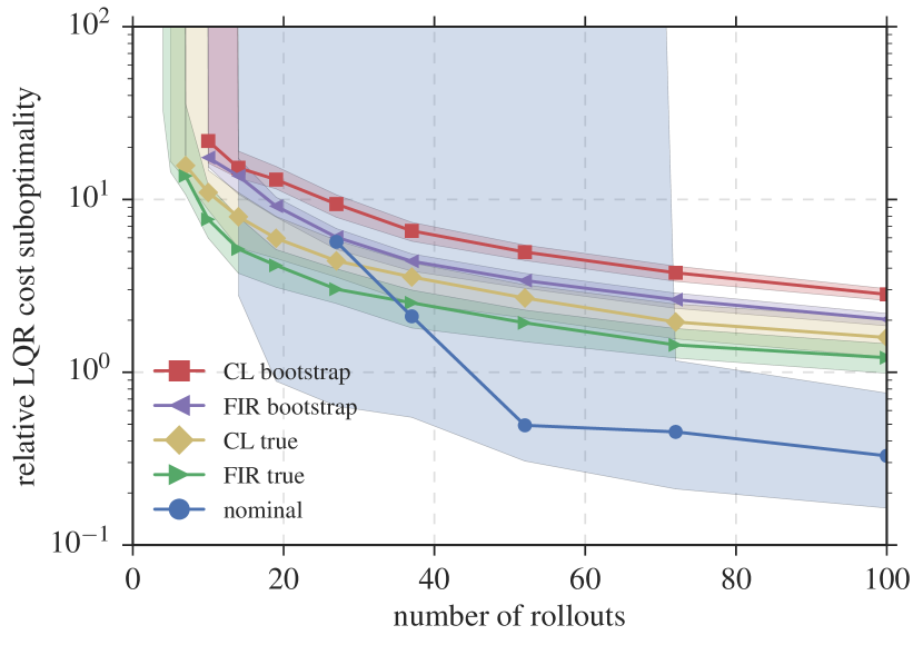
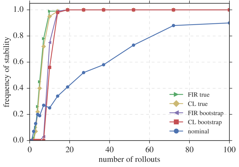
(a) LQR Cost Suboptimality

Refer to caption

(b) Frequency of Finding Stabilizing Controller

Refer to caption

Figure 2: The performance of controllers synthesized on the results of the 100 identification experiments is plotted against the number of rollouts. Controllers are synthesis nominally, using FIR truncation, and using the common Lyapunov (CL) relaxation. In (a), the median suboptimality of nominal and robustly synthesized controllers are compared, with shaded regions displaying quartiles, which go off to infinity in the case that a stabilizing controller was not found. In (b), the frequency that the synthesis methods found stabilizing controllers.
(a) LQR Cost Suboptimality Bound

Refer to caption

(b) LQR Cost Suboptimality

Refer to caption

Figure 3: The performance of controllers synthesized with varying FIR filter lengths on the results of 10 of the identification experiments using true errors. The median suboptimality of robustly synthesized controllers does not appear to change for FIR lengths greater than 32, and the common Lyapunov (CL) synthesis tracks the performance in both upper bound and actual cost.

LQR Cost Suboptimality

Refer to caption

Figure 4: The performance of controllers synthesized on the results of 100 identification experiments is plotted against the number of rollouts. The plot compares the median suboptimality of nominal controllers with fixed-γ𝛾\gamma robustly synthesized controllers (γ=0.999𝛾0.999\gamma=0.999).

7 Conclusions and Future Work

Coarse-ID control provides a straightforward approach to merging nonasymptotic methods from system identification with contemporary Systems Level Synthesis approaches to robust control. Indeed, many of the principles of Coarse-ID control were well established in the 90s [12, 13, 30], but fusing together an end-to-end result required contemporary analysis of random matrices and a new perspective on controller synthesis. These results can be extended in a variety of directions, and we close this paper with a discussion of some of the short-comings of our approach and of several possible applications of the Coarse-ID framework to other control settings.

Other performance metrics.

Though we focused exclusively on LQR in this paper, we note that all of our results on robust synthesis and end-to-end performance analysis extend to other metrics popular in control. Indeed, any norm on the system responses {Φx(k),Φu(k)}subscriptΦ𝑥𝑘subscriptΦ𝑢𝑘\{\Phi_{x}(k),\Phi_{u}(k)\} can be solved robustly using our approach; Lemma 3.4 holds for any norm. In turn, we can mimic the derivation in Section 3 to yield a constrained optimization problem with respect to the nominal dynamics and a norm on the uncertainty 𝚫^^𝚫\mathbf{\hat{\Delta}}. This means that our suboptimality bound in Corollary 4.3 holds true when we replace 2(𝕋)subscript2𝕋\mathcal{H}_{2}(\mathbb{T}) with (𝕋)subscript𝕋\mathcal{H}_{\infty}(\mathbb{T}). Furthermore, similar results can be derived for other norms, so long as care is placed on the associated submultiplicative properties of the norms in question. For example, in follow up work we analyze robustness under the 1subscript1\mathcal{L}_{1} norm in the context of constraints on the states and control signals [15].

Improving the end-to-end analysis.

There are several places where our analysis could be substantially improved. The most obvious is that in our estimator for the state-transition matrices, our algorithm only uses the final time step of each rollout. This strategy is data inefficient, and empirically, accuracy only improves when including all of the data. Analyzing the full least squares estimator is non-trivial because the design matrix strongly depends on data to be estimated. This poses a challenging problem in random matrix theory that has applications in a variety of control and reinforcement learning settings. In follow up work we have begun to address this issue for stable linear systems [52].

In the context of SLS, we use a very coarse characterization of the plant uncertainty to bound the quantity in Lemma 3.4 and to yield a tractable optimization problem. Indeed, the only property we use about the error between our nominal system and the true system is that the maps

x(AA^)xandu(BB^)umaps-to𝑥𝐴^𝐴𝑥and𝑢maps-to𝐵^𝐵𝑢x\mapsto(A-\hat{A})x~{}~{}\mbox{and}~{}~{}u\mapsto(B-\hat{B})u

are contractions. Nowhere do we use the fact that these are linear operators, or even the fact that they are the same operator from time-step to time-step. Indeed, there are stronger bounds that could be engineered using the theory of Integral Quadratic Constraints [41] that would take into account these additional properties. Such tighter bounds could yield considerably less conservative control schemes in both theory and practice.

Additionally, it would be of interest to understand the loss in performance incurred by the common Lyapunov relaxation we use in our experiments. Empirically, we see that the approximation leads to good performance, suggesting that it does not introduce much conservatism into the synthesis task. Further, our numerical experiments suggest that optimizing a nominal cost subject to robust stability constraints, as opposed to directly optimizing the SLS upper bound, leads to better empirical performance. Future work will seek to understand whether this is a phenomenological observation specific to the systems used in our experiments, or if there is a deeper principle at play that leads to tighter sub-optimality guarantees.

Lower bounds.

Finding lower bounds for control problems when the model is unknown is an open question. Even for LQR, it is not at all clear how well the system (A,B)𝐴𝐵(A,B) needs to be known in order to attain good control performance. While we produce reasonable worst-case upper bounds for this problem, we know of no lower bounds. Such bounds would offer a reasonable benchmark for how well one could ever expect to do with no priors on the linear system dynamics.

Integrating Coarse-ID control in other control paradigms.

The end-to-end Coarse-ID control framework should be applicable in a variety of settings. For example, in Model Predictive Control (MPC), controller synthesis problems are approximately solved on finite time horizons, one step is taken, and then this process is repeated [7]. MPC is an effective solution which substitutes fast optimization solvers for clever, complex control design. We believe it will be straightforward to extend the Coarse-ID paradigm to MPC, using a similar perturbation argument as in Section 3. The main challenges in MPC lie in how to guarantee that safety constraints are maintained throughout execution without too much conservatism in control costs.

Another interesting investigation lies in the area of adaptive control, where we could investigate how to incorporate new data into coarse models to further refine constraint sets and costs. Indeed, some work has already been done in this space. We propose to investigate how to operationalize and extend the notion of optimistic exploration proposed in the context of continuous control by Abbasi-Yadkori and Szepesvari [1]. The idea behind optimistic improvement is to select the model that would give the best optimization cost if the current model was true. In this way, we fail fast, either receiving a good cost or learning quickly that our model is incorrect. It would be worth investigating whether the Coarse-ID framework can make it simple to update a least squares estimate for the system parameters and then provide an efficient mechanism for choosing the next optimistic control.

Finally, Coarse-ID control could be relevant to nonlinear control applications. In nonlinear control, iterative LQR schemes are remarkably effective [36]. Hence, it would be interesting to understand how parametric model errors can be estimated and mitigated in a control loop that employs iterative LQR or similar dynamic programming methods.

Sample complexities of reinforcement learning for continuous control.

Finally, we imagine that the analysis in this paper may be useful for understanding popular reinforcement learning algorithms that are also being tested for continuous control. Reinforcement learning directly attacks a control cost in question without resorting to any specific identification scheme. While this suffers from the drawback that generally speaking, no parameter convergence can be guaranteed, it is ideally suited to ignoring modes that do not affect control performance. For instance, it might not be important to get a good estimate of very stable modes or of lightly damped modes that do not substantially affect the performance.

There are two parallel problems here. First, it would be of interest to determine system identification algorithms that are tuned to particular control tasks. In the Coarse-ID control approach, the estimation and control are completely decoupled. However, it may be beneficial to inform the identification algorithm about the desired cost, resulting in improved sample complexity.

From a different perspective, Policy Gradient and Q-Learning methods applied to LQR could yield important insights about the pros and cons of such methods. There are classic papers [10] on Q-Learning for LQR, but these use asymptotic analysis. Recently, the first such analysis for Policy Gradient has appeared, though the precise scaling with respect to system parameters is not yet understood [21]. Providing clean nonasymptotic bounds here could help provide a rapprochement between machine learning and adaptive control, with optimization negotiating the truce.

Acknowledgements

We thank Ross Boczar, Qingqing Huang, Laurent Lessard, Michael Littman, Manfred Morari, Andrew Packard, Anders Rantzer, Daniel Russo, and Ludwig Schmidt for many helpful comments and suggestions. We also thank the anonymous referees for making several suggestions that have significantly improved the paper and its presentation. SD is supported by an NSF Graduate Research Fellowship under Grant No. DGE 1752814. NM is generously funded by grants from the AFOSR and NSF, and by gifts from Huawei and Google. BR is generously supported by NSF award CCF-1359814, ONR awards N00014-14-1-0024 and N00014-17-1-2191, the DARPA Fundamental Limits of Learning (Fun LoL) Program, a Sloan Research Fellowship, and a Google Faculty Award.

References

  • Abbasi-Yadkori and Szepesvári [2011] Y. Abbasi-Yadkori and C. Szepesvári. Regret Bounds for the Adaptive Control of Linear Quadratic Systems. In Conference on Learning Theory, 2011.
  • Abeille and Lazaric [2017] M. Abeille and A. Lazaric. Thompson Sampling for Linear-Quadratic Control Problems. In AISTATS, 2017.
  • Abeille and Lazaric [2018] M. Abeille and A. Lazaric. Improved Regret Bounds for Thompson Sampling in Linear Quadratic Control Problems. In International Conference on Machine Learning, 2018.
  • Anderson and Matni [2017] J. Anderson and N. Matni. Structured State Space Realizations for SLS Distributed Controllers. In Allerton, 2017.
  • ApS [2015] M. ApS. The MOSEK optimization toolbox for MATLAB manual. Version 8.1 (Revision 25)., 2015. URL http://docs.mosek.com/8.1/toolbox/index.html.
  • Bento et al. [2010] J. Bento, M. Ibrahimi, and A. Montanari. Learning Networks of Stochastic Differential Equations. In Neural Information Processing Systems, 2010.
  • Borrelli et al. [2017] F. Borrelli, A. Bemporad, and M. Morari. Predictive Control for Linear and Hybrid Systems. 2017.
  • Box et al. [2008] G. E. P. Box, G. M. Jenkins, and G. C. Reinsel. Time Series Analysis: Forecasting and Control. 2008.
  • Braatz et al. [1994] R. P. Braatz, P. M. Young, J. C. Doyle, and M. Morari. Computational Complexity of μ𝜇\mu Calculation. IEEE Transactions on Automatic Control, 39(5), 1994.
  • Bradtke et al. [1994] S. J. Bradtke, B. E. Ydstie, and A. G. Barto. Adaptive linear quadratic control using policy iteration. In American Control Conference, 1994.
  • Campi and Weyer [2002] M. C. Campi and E. Weyer. Finite Sample Properties of System Identification Methods. IEEE Transactions on Automatic Control, 47(8), 2002.
  • Chen and Gu [2000] J. Chen and G. Gu. Control-Oriented System Identification: An subscript\mathcal{H}_{\infty} Approach. 2000.
  • Chen and Nett [1993] J. Chen and C. N. Nett. The Carathéodory-Fejér Problem and subscript\mathcal{H}_{\infty} Identification: A Time Domain Approach. In IEEE Conference on Decision and Control, 1993.
  • Dahleh and Diaz-Bobillo [1994] M. A. Dahleh and I. J. Diaz-Bobillo. Control of Uncertain Systems: A Linear Programming Approach. 1994.
  • Dean et al. [2018] S. Dean, S. Tu, N. Matni, and B. Recht. Safely Learning to Control the Constrained Linear Quadratic Regulator. arXiv:1809.10121, 2018.
  • Doyle [1982] J. Doyle. Analysis of feedback systems with structured uncertainties. IEE Proceedings D - Control Theory and Applications, 129(6), 1982. ISSN 0143-7054. doi: 10.1049/ip-d.1982.0053.
  • Duan et al. [2016] Y. Duan, X. Chen, R. Houthooft, J. Schulman, and P. Abbeel. Benchmarking Deep Reinforcement Learning for Continuous Control. In International Conference on Machine Learning, 2016.
  • Dumitrescu [2007] B. Dumitrescu. Positive trigonometric polynomials and signal processing applications. 2007.
  • Efron [1979] B. Efron. Bootstrap Methods: Another Look at the Jackknife. The Annals of Statistics, 7(1), 1979.
  • Fan et al. [1991] M. K. H. Fan, A. L. Tits, and J. C. Doyle. Robustness in the presence of mixed parametric uncertainty and unmodeled dynamics. IEEE Transactions on Automatic Control, 36(1), 1991. ISSN 0018-9286. doi: 10.1109/9.62265.
  • Fazel et al. [2018] M. Fazel, R. Ge, S. M. Kakade, and M. Mesbahi. Global Convergence of Policy Gradient Methods for the Linear Quadratic Regulator . In International Conference on Machine Learning, 2018.
  • Feron [1997] E. Feron. Analysis of Robust 2subscript2\mathcal{H}_{2} Performance Using Multiplier Theory. SIAM Journal on Control and Optimization, 35(1), 1997.
  • Fiechter [1997] C.-N. Fiechter. PAC Adaptive Control of Linear Systems. In Conference on Learning Theory, 1997.
  • Goldenshluger [1998] A. Goldenshluger. Nonparametric Estimation of Transfer Functions: Rates of Convergence and Adaptation. IEEE Transactions on Information Theory, 44(2), 1998.
  • Goldenshluger and Zeevi [2001] A. Goldenshluger and A. Zeevi. Nonasymptotic bounds for autoregressive time series modeling. The Annals of Statistics, 29(2), 2001.
  • Hall [2013] P. Hall. The Bootstrap and Edgeworth Expansion. Springer Science & Business Media, 2013.
  • Hardt et al. [2016] M. Hardt, T. Ma, and B. Recht. Gradient Descent Learns Linear Dynamical Systems. arXiv:1609.05191, 2016.
  • Hazan et al. [2017] E. Hazan, K. Singh, and C. Zhang. Learning Linear Dynamical Systems via Spectral Filtering. In Neural Information Processing Systems, 2017.
  • Hazan et al. [2018] E. Hazan, H. Lee, K. Singh, C. Zhang, and Y. Zhang. Spectral Filtering for General Linear Dynamical Systems. arXiv:1802.03981, 2018.
  • Helmicki et al. [1991] A. J. Helmicki, C. A. Jacobson, and C. N. Nett. Control Oriented System Identification: A Worst-Case/Deterministic Approach in subscript\mathcal{H}_{\infty}. IEEE Transactions on Automatic Control, 36(10), 1991.
  • Ibrahimi et al. [2012] M. Ibrahimi, A. Javanmard, and B. V. Roy. Efficient Reinforcement Learning for High Dimensional Linear Quadratic Systems. In Neural Information Processing Systems, 2012.
  • Jiang et al. [2017] N. Jiang, A. Krishnamurthy, A. Agarwal, J. Langford, and R. E. Schapire. Contextual Decision Processes with Low Bellman Rank are PAC-Learnable. In International Conference on Machine Learning, 2017.
  • Jonas et al. [2017] E. Jonas, Q. Pu, S. Venkataraman, I. Stoica, and B. Recht. Occupy the Cloud: Distributed Computing for the 99%. In ACM Symposium on Cloud Computing, 2017.
  • Kuznetsov and Mohri [2017] V. Kuznetsov and M. Mohri. Generalization bounds for non-stationary mixing processes. Machine Learning, 106(1), 2017.
  • Levine et al. [2016] S. Levine, C. Finn, T. Darrell, and P. Abbeel. End-to-End Training of Deep Visuomotor Policies. Journal of Machine Learning Research, 17(39), 2016.
  • Li and Todorov [2004] W. Li and E. Todorov. Iterative Linear Quadratic Regulator Design for Nonlinear Biological Movement Systems. In International Conference on Informatics in Control, Automation and Robotics, 2004.
  • Ljung [1999] L. Ljung. System Identification: Theory for the User. 1999.
  • Löfberg [2004] J. Löfberg. YALMIP : A toolbox for modeling and optimization in MATLAB. In IEEE International Symposium on Computer Aided Control System Design, 2004.
  • Matni et al. [2017] N. Matni, Y.-S. Wang, and J. Anderson. Scalable system level synthesis for virtually localizable systems. In IEEE Conference on Decision and Control, 2017.
  • McDonald et al. [2017] D. J. McDonald, C. R. Shalizi, and M. Schervish. Nonparametric Risk Bounds for Time-Series Forecasting. Journal of Machine Learning Research, 18, 2017.
  • Megretski and Rantzer [1997] A. Megretski and A. Rantzer. System analysis via integral quadratic constraints. IEEE Transactions on Automatic Control, 42(6), 1997.
  • Mnih et al. [2015] V. Mnih, K. Kavukcuoglu, D. Silver, A. A. Rusu, J. Veness, M. G. Bellemare, A. Graves, M. Riedmiller, A. K. Fidjeland, G. Ostrovski, S. Petersen, C. Beattie, A. Sadik, I. Antonoglou, H. King, D. Kumaran, D. Wierstra, S. Legg, D. H. I. Antonoglou, D. Wierstra, and M. A. Riedmiller. Human-level control through deep reinforcement learning. Nature, 2015.
  • Mohri and Rostamizadeh [2010] M. Mohri and A. Rostamizadeh. Stability Bounds for Stationary φ𝜑\varphi-mixing and β𝛽\beta-mixing Processes. Journal of Machine Learning Research, 11, 2010.
  • Ouyang et al. [2017] Y. Ouyang, M. Gagrani, and R. Jain. Control of Unknown Linear Systems with Thompson Sampling. In Allerton, 2017.
  • Packard and Doyle [1993] A. Packard and J. Doyle. The Complex Structured Singular Value. Automatica, 29(1), 1993.
  • Paganini [1995] F. Paganini. Necessary and Sufficient Conditions for Robust 2subscript2\mathcal{H}_{2} Performance. In IEEE Conference on Decision and Control, 1995.
  • Postoyan et al. [2017] R. Postoyan, L. Buşoniu, D. Nešić, and J. Daafouz. Stability Analysis of Discrete-Time Infinite-Horizon Optimal Control With Discounted Cost. IEEE Transactions on Automatic Control, 62(6), 2017.
  • Qiu et al. [1995] L. Qiu, B. Bernhardsson, A. Rantzer, E. J. Davison, P. Young, and J. Doyle. A formula for computation of the real stability radius. Automatica, 31(6):879–890, 1995.
  • Russo et al. [2017] D. Russo, B. V. Roy, A. Kazerouni, and I. Osband. A Tutorial on Thompson Sampling. arXiv:1707.02038, 2017.
  • Shao and Tu [2012] J. Shao and D. Tu. The Jackknife and Bootstrap. Springer Science & Business Media, 2012.
  • Silver et al. [2016] D. Silver, A. Huang, C. J. Maddison, A. Guez, L. Sifre, G. van den Driessche, J. Schrittwieser, I. Antonoglou, V. Panneershevlvam, M. Lanctot, S. Dieleman, D. Grewe, J. Nham, N. Kalchbrenner, I. Sutskever, T. Lillicrap, M. Leach, K. Kavukcuoglu, T. Graepel, and D. Hassabis. Mastering the game of go with deep neural networks and tree search. Nature, 2016.
  • Simchowitz et al. [2018] M. Simchowitz, H. Mania, S. Tu, M. I. Jordan, and B. Recht. Learning Without Mixing: Towards A Sharp Analysis of Linear System Identification. 2018.
  • Sznaier et al. [2002] M. Sznaier, T. Amishima, P. A. Parrilo, and J. Tierno. A convex approach to robust 2subscript2\mathcal{H}_{2} performance analysis. Automatica, 38(6), 2002.
  • Tu et al. [2017] S. Tu, R. Boczar, A. Packard, and B. Recht. Non-Asymptotic Analysis of Robust Control from Coarse-Grained Identification. arXiv:1707.04791, 2017.
  • Van Der Vaart and Wellner [1996] A. W. Van Der Vaart and J. A. Wellner. Weak Convergence and Empirical Processes. 1996.
  • Vershynin [2010] R. Vershynin. Introduction to the non-asymptotic analysis of random matrices. arXiv:1011.3027, 2010.
  • Vidyasagar and Karandikar [2008] M. Vidyasagar and R. L. Karandikar. A learning theory approach to system identification and stochastic adaptive control. Journal of Process Control, 18(3), 2008.
  • Wainwright [2019] M. J. Wainwright. High-dimensional Statistics: A Non-Asymptotic Viewpoint. Cambridge University Press, 2019.
  • Wang et al. [2016] Y.-S. Wang, N. Matni, and J. C. Doyle. A System Level Approach to Controller Synthesis. arXiv:1610.04815, 2016.
  • Wu and Packard [1995] F. Wu and A. Packard. Optimal LQG performance of linear uncertain systems using state-feedback. In American Control Conference, 1995.
  • Youla et al. [1976] D. Youla, H. Jabr, and J. Bongiorno. Modern Wiener-Hopf design of optimal controllers–Part II: The multivariable case. IEEE Transactions on Automatic Control, 21(3), 1976.
  • Young et al. [1991] P. M. Young, M. P. Newlin, and J. C. Doyle. μ𝜇\mu Analysis with Real Parametric Uncertainty. In IEEE Conference on Decision and Control, 1991.
  • Yu [1994] B. Yu. Rates of Convergence for Empirical Processes of Stationary Mixing Sequences. The Annals of Probability, 22(1), 1994.
  • Zhou et al. [1995] K. Zhou, J. C. Doyle, and K. Glover. Robust and Optimal Control. 1995.

Appendix A Proof of Lemma 2.1

First, recall Bernstein’s lemma. Let X1,,Xpsubscript𝑋1subscript𝑋𝑝X_{1},...,X_{p} be zero-mean independent r.v.s satisfying the Orlicz norm bound Xiψ1Ksubscriptdelimited-∥∥subscript𝑋𝑖subscript𝜓1𝐾\lVert X_{i}\rVert_{\psi_{1}}\leq K. Then as long as p2log(1/δ)𝑝21𝛿p\geq 2\log(1/\delta), with probability at least 1δ1𝛿1-\delta,

i=1pXiK2nlog(1/δ).superscriptsubscript𝑖1𝑝subscript𝑋𝑖𝐾2𝑛1𝛿\displaystyle\sum_{i=1}^{p}X_{i}\leq K\sqrt{2n\log(1/\delta)}\>.

Next, let Q𝑄Q be an m×n𝑚𝑛m\times n matrix. Let u1,,uMεsubscript𝑢1subscript𝑢subscript𝑀𝜀u_{1},...,u_{M_{\varepsilon}} be a ε𝜀\varepsilon-net for the m𝑚m-dimensional 2subscript2\ell_{2} ball, and similarly let v1,,vNεsubscript𝑣1subscript𝑣subscript𝑁𝜀v_{1},...,v_{N_{\varepsilon}} be a ε𝜀\varepsilon covering for the n𝑛n-dimensional 2subscript2\ell_{2} ball. For each u2=1subscriptdelimited-∥∥𝑢21\lVert u\rVert_{2}=1 and v2=1subscriptdelimited-∥∥𝑣21\lVert v\rVert_{2}=1, let uisubscript𝑢𝑖u_{i}, vjsubscript𝑣𝑗v_{j} denote the elements in the respective nets such that uui2εsubscriptdelimited-∥∥𝑢subscript𝑢𝑖2𝜀\lVert u-u_{i}\rVert_{2}\leq\varepsilon and vvj2εsubscriptdelimited-∥∥𝑣subscript𝑣𝑗2𝜀\lVert v-v_{j}\rVert_{2}\leq\varepsilon. Then,

uQvsuperscript𝑢𝑄𝑣\displaystyle u^{*}Qv =(uui+ui)Qv=(uui)Qv+uiQ(vvj+vj)absentsuperscript𝑢subscript𝑢𝑖subscript𝑢𝑖𝑄𝑣superscript𝑢subscript𝑢𝑖𝑄𝑣superscriptsubscript𝑢𝑖𝑄𝑣subscript𝑣𝑗subscript𝑣𝑗\displaystyle=(u-u_{i}+u_{i})^{*}Qv=(u-u_{i})^{*}Qv+u_{i}^{*}Q(v-v_{j}+v_{j})
=(uui)Qv+uiQ(vvj)+uiQvj.absentsuperscript𝑢subscript𝑢𝑖𝑄𝑣superscriptsubscript𝑢𝑖𝑄𝑣subscript𝑣𝑗superscriptsubscript𝑢𝑖𝑄subscript𝑣𝑗\displaystyle=(u-u_{i})^{*}Qv+u_{i}^{*}Q(v-v_{j})+u_{i}^{*}Qv_{j}\>.

Hence,

uQv2εQ2+uiQvj2εQ2+max1iMε,1jNεuiQvj.superscript𝑢𝑄𝑣2𝜀subscriptdelimited-∥∥𝑄2superscriptsubscript𝑢𝑖𝑄subscript𝑣𝑗2𝜀subscriptdelimited-∥∥𝑄2subscriptformulae-sequence1𝑖subscript𝑀𝜀1𝑗subscript𝑁𝜀superscriptsubscript𝑢𝑖𝑄subscript𝑣𝑗\displaystyle u^{*}Qv\leq 2\varepsilon\lVert Q\rVert_{2}+u_{i}^{*}Qv_{j}\leq 2\varepsilon\lVert Q\rVert_{2}+\max_{1\leq i\leq M_{\varepsilon},1\leq j\leq N_{\varepsilon}}u_{i}^{*}Qv_{j}\>.

Since u,v𝑢𝑣u,v are arbitrary on the sphere,

Q2112εmax1iMε,1jNεuiQvj.subscriptdelimited-∥∥𝑄2112𝜀subscriptformulae-sequence1𝑖subscript𝑀𝜀1𝑗subscript𝑁𝜀superscriptsubscript𝑢𝑖𝑄subscript𝑣𝑗\displaystyle\lVert Q\rVert_{2}\leq\frac{1}{1-2\varepsilon}\max_{1\leq i\leq M_{\varepsilon},1\leq j\leq N_{\varepsilon}}u_{i}^{*}Qv_{j}\>.

Now we study the problem at hand. Choose ε=1/4𝜀14\varepsilon=1/4. By a standard volume comparison argument, we have that Mε9msubscript𝑀𝜀superscript9𝑚M_{\varepsilon}\leq 9^{m} and Nε9nsubscript𝑁𝜀superscript9𝑛N_{\varepsilon}\leq 9^{n}, and that

k=1Nfkgk22max1iMε,1jNεk=1N(uifk)(gkvj).subscriptdelimited-∥∥superscriptsubscript𝑘1𝑁subscript𝑓𝑘superscriptsubscript𝑔𝑘22subscriptformulae-sequence1𝑖subscript𝑀𝜀1𝑗subscript𝑁𝜀superscriptsubscript𝑘1𝑁superscriptsubscript𝑢𝑖subscript𝑓𝑘superscriptsubscript𝑔𝑘subscript𝑣𝑗\displaystyle\left\lVert\sum_{k=1}^{N}f_{k}g_{k}^{*}\right\rVert_{2}\leq 2\max_{1\leq i\leq M_{\varepsilon},1\leq j\leq N_{\varepsilon}}\sum_{k=1}^{N}(u_{i}^{*}f_{k})(g_{k}^{*}v_{j})\>.

Note that uifkN(0,uiΣfui)similar-tosuperscriptsubscript𝑢𝑖subscript𝑓𝑘𝑁0superscriptsubscript𝑢𝑖subscriptΣ𝑓subscript𝑢𝑖u_{i}^{*}f_{k}\sim N(0,u_{i}^{*}\Sigma_{f}u_{i}) and gkvjN(0,vjΣgvj)similar-tosuperscriptsubscript𝑔𝑘subscript𝑣𝑗𝑁0superscriptsubscript𝑣𝑗subscriptΣ𝑔subscript𝑣𝑗g_{k}^{*}v_{j}\sim N(0,v_{j}^{*}\Sigma_{g}v_{j}). By independence of fksubscript𝑓𝑘f_{k} and gksubscript𝑔𝑘g_{k}, (uifk)(gkvj)superscriptsubscript𝑢𝑖subscript𝑓𝑘superscriptsubscript𝑔𝑘subscript𝑣𝑗(u_{i}^{*}f_{k})(g_{k}^{*}v_{j}) is a zero mean sub-Exponential random variable, and therefore (uifk)(gkvj)ψ12Σf21/2Σg21/2subscriptdelimited-∥∥superscriptsubscript𝑢𝑖subscript𝑓𝑘superscriptsubscript𝑔𝑘subscript𝑣𝑗subscript𝜓12superscriptsubscriptdelimited-∥∥subscriptΣ𝑓212superscriptsubscriptdelimited-∥∥subscriptΣ𝑔212\lVert(u_{i}^{*}f_{k})(g_{k}^{*}v_{j})\rVert_{\psi_{1}}\leq\sqrt{2}\lVert\Sigma_{f}\rVert_{2}^{1/2}\lVert\Sigma_{g}\rVert_{2}^{1/2}. Hence, for each pair ui,vjsubscript𝑢𝑖subscript𝑣𝑗u_{i},v_{j} we have with probability at least 1δ/9m+n1𝛿superscript9𝑚𝑛1-\delta/9^{m+n},

k=1N(uifk)(gkvj)2Σf21/2Σg21/2N(m+n)log(9/δ).superscriptsubscript𝑘1𝑁superscriptsubscript𝑢𝑖subscript𝑓𝑘superscriptsubscript𝑔𝑘subscript𝑣𝑗2superscriptsubscriptdelimited-∥∥subscriptΣ𝑓212superscriptsubscriptdelimited-∥∥subscriptΣ𝑔212𝑁𝑚𝑛9𝛿\displaystyle\sum_{k=1}^{N}(u_{i}^{*}f_{k})(g_{k}^{*}v_{j})\leq 2\lVert\Sigma_{f}\rVert_{2}^{1/2}\lVert\Sigma_{g}\rVert_{2}^{1/2}\sqrt{N(m+n)\log(9/\delta)}\>.

Taking a union bound over all pairs in the ε𝜀\varepsilon-net yields the claim.

Appendix B Proof of Proposition 2.4

For this proof we need a lemma similar to Lemma 2.1. The following is a standard result in high-dimensional statistics [58], and we state it here without proof.

Lemma B.1.

Let WN×n𝑊superscript𝑁𝑛W\in\mathbb{R}^{N\times n} be a matrix with each entry i.i.d. 𝒩(0,σw2)𝒩0superscriptsubscript𝜎𝑤2\mathcal{N}(0,\sigma_{w}^{2}). Then, with probability 1δ1𝛿1-\delta, we have

W2σw(N+n+2log(1/δ)).subscriptnorm𝑊2subscript𝜎𝑤𝑁𝑛21𝛿\displaystyle\|W\|_{2}\leq\sigma_{w}(\sqrt{N}+\sqrt{n}+\sqrt{2\log(1/\delta)}).

As before we use Z𝑍Z to denote the N×(n+p)𝑁𝑛𝑝N\times(n+p) matrix with rows equal to z=[(x())(u())]superscriptsubscript𝑧topmatrixsuperscriptsuperscript𝑥topsuperscriptsuperscript𝑢topz_{\ell}^{\top}=\begin{bmatrix}(x^{(\ell)})^{\top}&(u^{(\ell)})^{\top}\end{bmatrix}. Also, we denote by W𝑊W the N×n𝑁𝑛N\times n matrix with columns equal to w()superscript𝑤w^{(\ell)}. Therefore, the error matrix for the ordinary least squares estimator satisfies

E=[(A^A)(B^B)]=(ZZ)1ZW,𝐸matrixsuperscript^𝐴𝐴topsuperscript^𝐵𝐵topsuperscriptsuperscript𝑍top𝑍1superscript𝑍top𝑊\displaystyle E=\begin{bmatrix}(\widehat{A}-A)^{\top}\\ (\widehat{B}-B)^{\top}\end{bmatrix}=(Z^{\top}Z)^{-1}Z^{\top}W,

when the matrix Z𝑍Z has rank n+p𝑛𝑝n+p. Under the assumption that Nn+p𝑁𝑛𝑝N\geq n+p we consider the singular value decomposition Z=UΛV𝑍𝑈Λsuperscript𝑉topZ=U\Lambda V^{\top}, where V,Λ(n+p)×(n+p)𝑉Λsuperscript𝑛𝑝𝑛𝑝V,\Lambda\in\mathbb{R}^{(n+p)\times(n+p)} and UN×(n+p)𝑈superscript𝑁𝑛𝑝U\in\mathbb{R}^{N\times(n+p)}. Therefore, when ΛΛ\Lambda is invertible,

E=V(ΛΛ)1ΛUW=VΛ1UW.𝐸𝑉superscriptsuperscriptΛtopΛ1superscriptΛtopsuperscript𝑈top𝑊𝑉superscriptΛ1superscript𝑈top𝑊\displaystyle E=V(\Lambda^{\top}\Lambda)^{-1}\Lambda^{\top}U^{\top}W=V\Lambda^{-1}U^{\top}W.

This implies that

EE𝐸superscript𝐸top\displaystyle EE^{\top} =VΛ1UWWUΛ1VUW22VΛ2V=UW22(ZZ)1.absent𝑉superscriptΛ1superscript𝑈top𝑊superscript𝑊top𝑈superscriptΛ1superscript𝑉topprecedes-or-equalssuperscriptsubscriptnormsuperscript𝑈top𝑊22𝑉superscriptΛ2superscript𝑉topsuperscriptsubscriptnormsuperscript𝑈top𝑊22superscriptsuperscript𝑍top𝑍1\displaystyle=V\Lambda^{-1}U^{\top}WW^{\top}U\Lambda^{-1}V^{\top}\preceq\|U^{\top}W\|_{2}^{2}V\Lambda^{-2}V^{\top}=\|U^{\top}W\|_{2}^{2}(Z^{\top}Z)^{-1}.

Since the columns of U𝑈U are orthonormal, it follows that the entries of UWsuperscript𝑈top𝑊U^{\top}W are i.i.d. 𝒩(0,σw2)𝒩0superscriptsubscript𝜎𝑤2\mathcal{N}(0,\sigma_{w}^{2}). Hence, the conclusion follows by Lemma B.1.

Appendix C Derivation of the LQR cost as an 2subscript2\mathcal{H}_{2} norm

In this section, we consider the transfer function description of the infinite horizon LQR optimal control problem. In particular, we show how it can be recast as an equivalent 2subscript2\mathcal{H}_{2} optimal control problem in terms of the system response variables defined in Theorem 3.1.

Recall that stable and achievable system responses (𝚽x,𝚽u)subscript𝚽𝑥subscript𝚽𝑢(\mathbf{\Phi}_{x},\mathbf{\Phi}_{u}), as characterized in equation (3.6), describe the closed-loop map from disturbance signal 𝐰𝐰\mathbf{w} to the state and control action (𝐱,𝐮)𝐱𝐮(\mathbf{x},\mathbf{u}) achieved by the controller 𝐊=𝚽u𝚽x1𝐊subscript𝚽𝑢superscriptsubscript𝚽𝑥1\mathbf{K}=\mathbf{\Phi}_{u}\mathbf{\Phi}_{x}^{-1}, i.e.,

[𝐱𝐮]=[𝚽x𝚽u]𝐰.matrix𝐱𝐮matrixsubscript𝚽𝑥subscript𝚽𝑢𝐰\begin{bmatrix}\mathbf{x}\\ \mathbf{u}\end{bmatrix}=\begin{bmatrix}\mathbf{\Phi}_{x}\\ \mathbf{\Phi}_{u}\end{bmatrix}\mathbf{w}.

Letting 𝚽x=t=1Φx(t)ztsubscript𝚽𝑥superscriptsubscript𝑡1subscriptΦ𝑥𝑡superscript𝑧𝑡\mathbf{\Phi}_{x}=\sum_{t=1}^{\infty}\Phi_{x}(t)z^{-t} and 𝚽u=t=1Φu(t)ztsubscript𝚽𝑢superscriptsubscript𝑡1subscriptΦ𝑢𝑡superscript𝑧𝑡\mathbf{\Phi}_{u}=\sum_{t=1}^{\infty}\Phi_{u}(t)z^{-t}, we can then equivalently write for any t1𝑡1t\geq 1

[xtut]=k=1t[Φx(k)Φu(k)]wtk.matrixsubscript𝑥𝑡subscript𝑢𝑡superscriptsubscript𝑘1𝑡matrixsubscriptΦ𝑥𝑘subscriptΦ𝑢𝑘subscript𝑤𝑡𝑘\begin{bmatrix}x_{t}\\ u_{t}\end{bmatrix}=\sum_{k=1}^{t}\begin{bmatrix}\Phi_{x}(k)\\ \Phi_{u}(k)\end{bmatrix}w_{t-k}. (C.1)

For a disturbance process distributed as wt i.i.d.𝒩(0,σw2In)superscriptsimilar-to i.i.d.subscript𝑤𝑡𝒩0superscriptsubscript𝜎𝑤2subscript𝐼𝑛w_{t}\stackrel{{\scriptstyle\mathclap{\text{\scriptsize{ \tiny i.i.d.}}}}}{{\sim}}\mathcal{N}(0,\sigma_{w}^{2}I_{n}), it follows from equation (C.1) that

𝔼[xtQxt]𝔼delimited-[]superscriptsubscript𝑥𝑡𝑄subscript𝑥𝑡\displaystyle\mathbb{E}\left[x_{t}^{*}Qx_{t}\right] =σw2k=1t𝐓𝐫(Φx(k)QΦx(k)),absentsuperscriptsubscript𝜎𝑤2superscriptsubscript𝑘1𝑡𝐓𝐫subscriptΦ𝑥superscript𝑘𝑄subscriptΦ𝑥𝑘\displaystyle=\sigma_{w}^{2}\sum_{k=1}^{t}\operatorname*{\mathbf{Tr}}(\Phi_{x}(k)^{*}Q\Phi_{x}(k))\>,
𝔼[utRut]𝔼delimited-[]superscriptsubscript𝑢𝑡𝑅subscript𝑢𝑡\displaystyle\mathbb{E}\left[u_{t}^{*}Ru_{t}\right] =σw2k=1t𝐓𝐫(Φu(k)RΦu(k)).absentsuperscriptsubscript𝜎𝑤2superscriptsubscript𝑘1𝑡𝐓𝐫subscriptΦ𝑢superscript𝑘𝑅subscriptΦ𝑢𝑘\displaystyle=\sigma_{w}^{2}\sum_{k=1}^{t}\operatorname*{\mathbf{Tr}}(\Phi_{u}(k)^{*}R\Phi_{u}(k))\>.

We can then write

limT1Tt=1T𝔼[xtQxt+utRut]subscript𝑇1𝑇superscriptsubscript𝑡1𝑇𝔼delimited-[]superscriptsubscript𝑥𝑡𝑄subscript𝑥𝑡superscriptsubscript𝑢𝑡𝑅subscript𝑢𝑡\displaystyle\lim_{T\to\infty}\frac{1}{T}\sum_{t=1}^{T}\mathbb{E}\left[x_{t}^{*}Qx_{t}+u_{t}^{*}Ru_{t}\right] =σw2[t=1𝐓𝐫(Φx(t)QΦx(t))+𝐓𝐫(Φu(t)RΦu(t))]absentsuperscriptsubscript𝜎𝑤2delimited-[]superscriptsubscript𝑡1𝐓𝐫subscriptΦ𝑥superscript𝑡𝑄subscriptΦ𝑥𝑡𝐓𝐫subscriptΦ𝑢superscript𝑡𝑅subscriptΦ𝑢𝑡\displaystyle=\sigma_{w}^{2}\left[\sum_{t=1}^{\infty}\operatorname*{\mathbf{Tr}}(\Phi_{x}(t)^{*}Q\Phi_{x}(t))+\operatorname*{\mathbf{Tr}}(\Phi_{u}(t)^{*}R\Phi_{u}(t))\right]
=σw2t=1[Q1200R12][Φx(t)Φu(t)]F2absentsuperscriptsubscript𝜎𝑤2superscriptsubscript𝑡1superscriptsubscriptdelimited-∥∥matrixsuperscript𝑄1200superscript𝑅12matrixsubscriptΦ𝑥𝑡subscriptΦ𝑢𝑡𝐹2\displaystyle=\sigma_{w}^{2}\sum_{t=1}^{\infty}\left\lVert\begin{bmatrix}Q^{\frac{1}{2}}&0\\ 0&R^{\frac{1}{2}}\end{bmatrix}\begin{bmatrix}\Phi_{x}(t)\\ \Phi_{u}(t)\end{bmatrix}\right\rVert_{F}^{2}
=σw22π𝕋[Q1200R12][𝚽x𝚽u]F2𝑑zabsentsuperscriptsubscript𝜎𝑤22𝜋subscript𝕋superscriptsubscriptdelimited-∥∥matrixsuperscript𝑄1200superscript𝑅12matrixsubscript𝚽𝑥subscript𝚽𝑢𝐹2differential-d𝑧\displaystyle=\frac{\sigma_{w}^{2}}{2\pi}\int_{\mathbb{T}}\left\lVert\begin{bmatrix}Q^{\frac{1}{2}}&0\\ 0&R^{\frac{1}{2}}\end{bmatrix}\begin{bmatrix}\mathbf{\Phi}_{x}\\ \mathbf{\Phi}_{u}\end{bmatrix}\right\rVert_{F}^{2}\;dz
=σw2[Q1200R12][𝚽x𝚽u]22,absentsuperscriptsubscript𝜎𝑤2superscriptsubscriptdelimited-∥∥matrixsuperscript𝑄1200superscript𝑅12matrixsubscript𝚽𝑥subscript𝚽𝑢subscript22\displaystyle=\sigma_{w}^{2}\left\lVert\begin{bmatrix}Q^{\frac{1}{2}}&0\\ 0&R^{\frac{1}{2}}\end{bmatrix}\begin{bmatrix}\mathbf{\Phi}_{x}\\ \mathbf{\Phi}_{u}\end{bmatrix}\right\rVert_{\mathcal{H}_{2}}^{2}\>,

where the second to last equality is due to Parseval’s Theorem.

Appendix D Proof of Theorem 5.1

To understand the effect of restricting the optimization to FIR transfer functions we need to understand the decay of the transfer functions A^+B^Ksubscript^𝐴^𝐵subscript𝐾\mathfrak{R}_{\widehat{A}+\widehat{B}K_{\star}} and KA^+B^Ksubscript𝐾subscript^𝐴^𝐵subscript𝐾K_{\star}\mathfrak{R}_{\widehat{A}+\widehat{B}K_{\star}}. To this end we consider C>0subscript𝐶0C_{\star}>0 and ρ(0,1)subscript𝜌01\rho_{\star}\in(0,1) such that (A+BK)t2Cρtsubscriptnormsuperscript𝐴𝐵subscript𝐾𝑡2subscript𝐶superscriptsubscript𝜌𝑡\|(A+BK_{\star})^{t}\|_{2}\leq C_{\star}\rho_{\star}^{t} for all t0𝑡0t\geq 0. Such Csubscript𝐶C_{\star} and ρsubscript𝜌\rho_{\star} exist because Ksubscript𝐾K_{\star} stabilizes the system (A,B)𝐴𝐵(A,B). The next lemma quantifies how well Ksubscript𝐾K_{\star} stabilizes the system (A^,B^)^𝐴^𝐵(\widehat{A},\widehat{B}) when the estimation error is small.

Lemma D.1.

Suppose ϵA+ϵBK21ρ2Csubscriptitalic-ϵ𝐴subscriptitalic-ϵ𝐵subscriptnormsubscript𝐾21subscript𝜌2subscript𝐶\epsilon_{A}+\epsilon_{B}\|K_{\star}\|_{2}\leq\frac{1-\rho_{\star}}{2C_{\star}}. Then,

(A^+B^K)t2C(1+ρ2)t, for all t0.subscriptnormsuperscript^𝐴^𝐵subscript𝐾𝑡2subscript𝐶superscript1subscript𝜌2𝑡, for all 𝑡0\displaystyle\|(\widehat{A}+\widehat{B}K_{\star})^{t}\|_{2}\leq C_{\star}\left(\frac{1+\rho_{\star}}{2}\right)^{t}\;\text{, for all }\;t\geq 0.
Proof.

The claim is obvious when t=0𝑡0t=0. Fix an integer t1𝑡1t\geq 1 and denote M=A+BK𝑀𝐴𝐵subscript𝐾M=A+BK_{\star}. Then, if Δ=ΔA+ΔBKΔsubscriptΔ𝐴subscriptΔ𝐵subscript𝐾\Delta=\Delta_{A}+\Delta_{B}K_{\star}, we have A^+B^K=M+Δ^𝐴^𝐵subscript𝐾𝑀Δ\widehat{A}+\widehat{B}K_{\star}=M+\Delta.

Consider the expansion of (M+Δ)tsuperscript𝑀Δ𝑡(M+\Delta)^{t} into 2ksuperscript2𝑘2^{k} terms. Label all these terms as Ti,jsubscript𝑇𝑖𝑗T_{i,j} for i=0,,t𝑖0𝑡i=0,...,t and j=1,,(ti)𝑗1binomial𝑡𝑖j=1,...,{t\choose i} where i𝑖i denotes the degree of ΔΔ\Delta in the term. Using the fact that Mt2Cρtsubscriptdelimited-∥∥superscript𝑀𝑡2subscript𝐶superscriptsubscript𝜌𝑡\lVert M^{t}\rVert_{2}\leq C_{\star}\rho_{\star}^{t} for all t0𝑡0t\geq 0, we have Ti,j2Ci+1ρtiΔ2isubscriptdelimited-∥∥subscript𝑇𝑖𝑗2superscript𝐶𝑖1superscript𝜌𝑡𝑖superscriptsubscriptdelimited-∥∥Δ2𝑖\lVert T_{i,j}\rVert_{2}\leq C^{i+1}\rho^{t-i}\lVert\Delta\rVert_{2}^{i}. Hence by triangle inequality:

(M+Δ)t2subscriptdelimited-∥∥superscript𝑀Δ𝑡2\displaystyle\lVert(M+\Delta)^{t}\rVert_{2} i=0tjTi,j2absentsuperscriptsubscript𝑖0𝑡subscript𝑗subscriptdelimited-∥∥subscript𝑇𝑖𝑗2\displaystyle\leq\sum_{i=0}^{t}\sum_{j}\lVert T_{i,j}\rVert_{2}
i=0t(ti)Ci+1ρtiΔ2iabsentsuperscriptsubscript𝑖0𝑡binomial𝑡𝑖superscriptsubscript𝐶𝑖1superscriptsubscript𝜌𝑡𝑖subscriptsuperscriptdelimited-∥∥Δ𝑖2\displaystyle\leq\sum_{i=0}^{t}{t\choose i}C_{\star}^{i+1}\rho_{\star}^{t-i}\lVert\Delta\rVert^{i}_{2}
=Ci=0t(ti)(CΔ2)iρtiabsentsubscript𝐶superscriptsubscript𝑖0𝑡binomial𝑡𝑖superscriptsubscript𝐶subscriptdelimited-∥∥Δ2𝑖superscriptsubscript𝜌𝑡𝑖\displaystyle=C_{\star}\sum_{i=0}^{t}{t\choose i}(C_{\star}\lVert\Delta\rVert_{2})^{i}\rho_{\star}^{t-i}
=C(CΔ2+ρ)tabsentsubscript𝐶superscriptsubscript𝐶subscriptdelimited-∥∥Δ2subscript𝜌𝑡\displaystyle=C_{\star}(C_{\star}\lVert\Delta\rVert_{2}+\rho_{\star})^{t}
C(1+ρ2)t,absentsubscript𝐶superscript1subscript𝜌2𝑡\displaystyle\leq C_{\star}\left(\frac{1+\rho_{\star}}{2}\right)^{t}\>,

where the last inequality uses the fact Δ2ϵA+ϵBK21ρ2Csubscriptdelimited-∥∥Δ2subscriptitalic-ϵ𝐴subscriptitalic-ϵ𝐵subscriptdelimited-∥∥subscript𝐾21subscript𝜌2subscript𝐶\lVert\Delta\rVert_{2}\leq\epsilon_{A}+\epsilon_{B}\lVert K_{\star}\rVert_{2}\leq\frac{1-\rho_{\star}}{2C_{\star}}. ∎

For the remainder of this discussion, we use the following notation to denote the restriction of a system response to its first L𝐿L time-steps:

𝚽x(1:L)=t=1L1ztΦx(t),𝚽u(1:L)=t=1L1ztΦu(t).\mathbf{\Phi}_{x}(1:L)=\sum_{t=1}^{L}\frac{1}{z^{t}}\Phi_{x}(t),\ \mathbf{\Phi}_{u}(1:L)=\sum_{t=1}^{L}\frac{1}{z^{t}}\Phi_{u}(t). (D.1)

To prove Theorem 5.1 we must relate the optimal controller Ksubscript𝐾K_{\star} with the optimal solution of the optimization problem (5.2). In the next lemma we use Ksubscript𝐾K_{\star} to construct a feasible solution for problem (5.2). As before, we denote ζ=(ϵA+ϵBK2)A+BK𝜁subscriptitalic-ϵ𝐴subscriptitalic-ϵ𝐵subscriptdelimited-∥∥subscript𝐾2subscriptnormsubscript𝐴𝐵subscript𝐾subscript\zeta=(\epsilon_{A}+\epsilon_{B}\lVert K_{\star}\rVert_{2})\|\mathfrak{R}_{A+BK_{\star}}\|_{\mathcal{H}_{\infty}}.

Lemma D.2.

Set α=1/2𝛼12\alpha=1/2 in problem (5.2), and assume that ϵA+ϵBK21ρ2Csubscriptitalic-ϵ𝐴subscriptitalic-ϵ𝐵subscriptnormsubscript𝐾21subscript𝜌2subscript𝐶\epsilon_{A}+\epsilon_{B}\|K_{\star}\|_{2}\leq\frac{1-\rho_{\star}}{2C_{\star}}, ζ<1/5𝜁15\zeta<1/5, and

L4log(Cζ)1ρ.𝐿4subscript𝐶𝜁1subscript𝜌L\geq\frac{4\log\left(\frac{C_{\star}}{\zeta}\right)}{1-\rho_{\star}}. (D.2)

Then, optimization problem (5.2) is feasible, and the following is one such feasible solution:

𝚽~x=A^+B^K(1:L),𝚽~u=KA^+B^K(1:L),V~=A^+B^K(L+1),γ~=4ζ1ζ.\widetilde{\mathbf{\Phi}}_{x}=\mathfrak{R}_{\widehat{A}+\widehat{B}K_{\star}}(1:L),~{}~{}\widetilde{\mathbf{\Phi}}_{u}=K_{\star}\mathfrak{R}_{\widehat{A}+\widehat{B}K_{\star}}(1:L),~{}~{}\widetilde{V}=-\mathfrak{R}_{\widehat{A}+\widehat{B}K_{\star}}(L+1),~{}~{}\tilde{\gamma}=\frac{4\zeta}{1-\zeta}. (D.3)
Proof.

From Lemma D.1 and the assumption on ζ𝜁\zeta we have that (A^+B^K)t2C(1+ρ2)tsubscriptdelimited-∥∥superscript^𝐴^𝐵subscript𝐾𝑡2subscript𝐶superscript1subscript𝜌2𝑡\lVert(\widehat{A}+\widehat{B}K_{\star})^{t}\rVert_{2}\leq C_{\star}\left(\frac{1+\rho_{\star}}{2}\right)^{t} for all t0𝑡0t\geq 0. In particular, since A^+B^K(L+1)=(A^+B^K)Lsubscript^𝐴^𝐵subscript𝐾𝐿1superscript^𝐴^𝐵subscript𝐾𝐿\mathfrak{R}_{\widehat{A}+\widehat{B}K_{\star}}(L+1)=(\widehat{A}+\widehat{B}K_{\star})^{L}, we have V~=(A^+B^K)LC(1+ρ2)Lζdelimited-∥∥~𝑉delimited-∥∥superscript^𝐴^𝐵subscript𝐾𝐿subscript𝐶superscript1subscript𝜌2𝐿𝜁\lVert\widetilde{V}\rVert=\lVert(\widehat{A}+\widehat{B}K_{\star})^{L}\rVert\leq C_{\star}\left(\frac{1+\rho_{\star}}{2}\right)^{L}\leq\zeta. The last inequality is true because we assumed L𝐿L is sufficiently large.

Once again, since A^+B^K(L+1)=(A^+B^K)Lsubscript^𝐴^𝐵subscript𝐾𝐿1superscript^𝐴^𝐵subscript𝐾𝐿\mathfrak{R}_{\widehat{A}+\widehat{B}K_{\star}}(L+1)=(\widehat{A}+\widehat{B}K_{\star})^{L}, it can be easily seen that our choice of 𝚽~xsubscript~𝚽𝑥\widetilde{\mathbf{\Phi}}_{x}, 𝚽~usubscript~𝚽𝑢\widetilde{\mathbf{\Phi}}_{u}, and V~~𝑉\widetilde{V} satisfy the linear constraint of problem (5.2). It remains to prove that

2[ϵA𝚽xϵB𝚽u]+V~2γ~<1.2subscriptnormmatrixsubscriptitalic-ϵ𝐴subscript𝚽𝑥subscriptitalic-ϵ𝐵subscript𝚽𝑢subscriptsubscriptdelimited-∥∥~𝑉2~𝛾1\displaystyle\sqrt{2}\left\|\begin{bmatrix}{\epsilon_{A}}{\mathbf{\Phi}_{x}}\\ {\epsilon_{B}}{\mathbf{\Phi}_{u}}\end{bmatrix}\right\|_{\mathcal{H}_{\infty}}+\lVert\widetilde{V}\rVert_{2}\leq\tilde{\gamma}<1.

The second inequality holds because of our assumption on ζ𝜁\zeta. We already know that V~2ζsubscriptdelimited-∥∥~𝑉2𝜁\lVert\widetilde{V}\rVert_{2}\leq\zeta. Now, we bound:

[ϵA𝚽~xϵB𝚽~u]subscriptnormmatrixsubscriptitalic-ϵ𝐴subscript~𝚽𝑥subscriptitalic-ϵ𝐵subscript~𝚽𝑢subscript\displaystyle\left\|\begin{bmatrix}{\epsilon_{A}}{\widetilde{\mathbf{\Phi}}_{x}}\\ {\epsilon_{B}}{\widetilde{\mathbf{\Phi}}_{u}}\end{bmatrix}\right\|_{\mathcal{H}_{\infty}} (ϵA+ϵBK2)A^+B^K(1:L)\displaystyle\leq(\epsilon_{A}+\epsilon_{B}\lVert K_{\star}\rVert_{2})\|\mathfrak{R}_{\widehat{A}+\widehat{B}K_{\star}}(1:L)\|_{\mathcal{H}_{\infty}}
(ϵA+ϵBK2)(A^+B^K+A^+B^K(L+1:)).\displaystyle\leq(\epsilon_{A}+\epsilon_{B}\lVert K_{\star}\rVert_{2})(\|\mathfrak{R}_{\widehat{A}+\widehat{B}K_{\star}}\|_{\mathcal{H}_{\infty}}+\|\mathfrak{R}_{\widehat{A}+\widehat{B}K_{\star}}(L+1:\infty)\|_{\mathcal{H}_{\infty}}).

These inequalities follow from the definition of (𝚽~x,𝚽~u)subscript~𝚽𝑥subscript~𝚽𝑢(\widetilde{\mathbf{\Phi}}_{x},\widetilde{\mathbf{\Phi}}_{u}) and the triangle inequality.

Now, we recall that A^+B^K=A+BK(I+𝚫)1subscript^𝐴^𝐵subscript𝐾subscript𝐴𝐵subscript𝐾superscript𝐼𝚫1\mathfrak{R}_{\widehat{A}+\widehat{B}K_{\star}}=\mathfrak{R}_{A+BK_{\star}}(I+\mathbf{\Delta})^{-1}, where 𝚫=(ΔA+ΔBK)A+BK𝚫subscriptΔ𝐴subscriptΔ𝐵subscript𝐾subscript𝐴𝐵subscript𝐾\mathbf{\Delta}=-(\Delta_{A}+\Delta_{B}K_{\star})\mathfrak{R}_{A+BK_{\star}}. Then, since 𝚫ζsubscriptnorm𝚫subscript𝜁\|\mathbf{\Delta}\|_{\mathcal{H}_{\infty}}\leq\zeta (due to Proposition 3.15), we have A^+B^K11ζA+BKsubscriptnormsubscript^𝐴^𝐵subscript𝐾subscript11𝜁subscriptnormsubscript𝐴𝐵subscript𝐾subscript\|\mathfrak{R}_{\widehat{A}+\widehat{B}K_{\star}}\|_{\mathcal{H}_{\infty}}\leq\frac{1}{1-\zeta}\|\mathfrak{R}_{A+BK_{\star}}\|_{\mathcal{H}_{\infty}}.

We can upper bound

A^+B^K(L+1:)t=L+1A^+B^K(t)2C(1+ρ2)Lt=0(1+ρ2)t=2C1ρ(1+ρ2)L.\displaystyle\|\mathfrak{R}_{\widehat{A}+\widehat{B}K_{\star}}(L+1:\infty)\|_{\mathcal{H}_{\infty}}\leq\sum_{t=L+1}^{\infty}\lVert\mathfrak{R}_{\widehat{A}+\widehat{B}K_{\star}}({t})\rVert_{2}\leq C_{\star}\left(\frac{1+\rho_{\star}}{2}\right)^{L}\sum_{t=0}^{\infty}\left(\frac{1+\rho_{\star}}{2}\right)^{t}=\frac{2C_{\star}}{1-\rho_{\star}}\left(\frac{1+\rho_{\star}}{2}\right)^{L}.

Then, since we assumed that ϵAsubscriptitalic-ϵ𝐴\epsilon_{A} and ϵBsubscriptitalic-ϵ𝐵\epsilon_{B} are sufficiently small and that L𝐿L is sufficiently large, we obatin

(ϵA+ϵBK2)A^+B^K(L+1:)ζ.\displaystyle(\epsilon_{A}+\epsilon_{B}\lVert K_{\star}\rVert_{2})\|\mathfrak{R}_{\widehat{A}+\widehat{B}K_{\star}}(L+1:\infty)\|_{\mathcal{H}_{\infty}}\leq\zeta.

Therefore,

[ϵA𝚽~xϵB𝚽~u]subscriptnormmatrixsubscriptitalic-ϵ𝐴subscript~𝚽𝑥subscriptitalic-ϵ𝐵subscript~𝚽𝑢subscript\displaystyle\left\|\begin{bmatrix}{\epsilon_{A}}{\widetilde{\mathbf{\Phi}}_{x}}\\ {\epsilon_{B}}{\widetilde{\mathbf{\Phi}}_{u}}\end{bmatrix}\right\|_{\mathcal{H}_{\infty}} ζ1ζ+ζ2ζ1ζ.absent𝜁1𝜁𝜁2𝜁1𝜁\displaystyle\leq\frac{\zeta}{1-\zeta}+\zeta\leq\frac{2\zeta}{1-\zeta}.

The conclusion follows. ∎

Proof of Theorem 5.1.

As all of the assumptions of Lemma D.2 are satisfied, optimization problem (5.2) is feasible. We denote (𝚽x,𝚽u,V,γ)superscriptsubscript𝚽𝑥superscriptsubscript𝚽𝑢subscript𝑉subscript𝛾(\mathbf{\Phi}_{x}^{\star},\mathbf{\Phi}_{u}^{\star},V_{\star},\gamma_{\star}) the optimal solution of problem (5.2). We denote

𝚫^:=ΔA𝚽x+ΔB𝚽u+1zLV.assign^𝚫subscriptΔ𝐴superscriptsubscript𝚽𝑥subscriptΔ𝐵superscriptsubscript𝚽𝑢1superscript𝑧𝐿subscript𝑉\hat{\mathbf{\Delta}}:=\Delta_{A}\mathbf{\Phi}_{x}^{\star}+\Delta_{B}\mathbf{\Phi}_{u}^{\star}+\frac{1}{z^{L}}V_{\star}.

Then, we have

[zIAB][𝚽x𝚽u]=I+𝚫^.matrix𝑧𝐼𝐴𝐵matrixsuperscriptsubscript𝚽𝑥superscriptsubscript𝚽𝑢𝐼^𝚫\displaystyle\begin{bmatrix}zI-A&-B\end{bmatrix}\begin{bmatrix}\mathbf{\Phi}_{x}^{\star}\\ \mathbf{\Phi}_{u}^{\star}\end{bmatrix}=I+\hat{\mathbf{\Delta}}.

Applying the triangle inequality, and leveraging Proposition 3.15, we can verify that

𝚫^2[ϵA𝚽xϵB𝚽u]+V2γ<1,subscriptnorm^𝚫subscript2subscriptnormmatrixsubscriptitalic-ϵ𝐴superscriptsubscript𝚽𝑥subscriptitalic-ϵ𝐵superscriptsubscript𝚽𝑢subscriptsubscriptdelimited-∥∥subscript𝑉2subscript𝛾1\|\hat{\mathbf{\Delta}}\|_{\mathcal{H}_{\infty}}\leq\sqrt{2}\left\|\begin{bmatrix}\epsilon_{A}\mathbf{\Phi}_{x}^{\star}\\ \epsilon_{B}\mathbf{\Phi}_{u}^{\star}\end{bmatrix}\right\|_{\mathcal{H}_{\infty}}+\lVert V_{\star}\rVert_{2}\leq\gamma_{\star}<1,

where the last two inequalities are true because the optimal solution is a feasible point of the optimization problem (5.2).

We now apply Lemma 3.4 to characterize the response achieved by the FIR approximate controller 𝐊Lsubscript𝐊𝐿\mathbf{K}_{L} on the true system (A,B)𝐴𝐵(A,B):

J(A,B,𝐊L)𝐽𝐴𝐵subscript𝐊𝐿\displaystyle J(A,B,\mathbf{K}_{L}) =[Q1200R12][𝚽x𝚽u](I+𝚫^)12absentsubscriptnormmatrixsuperscript𝑄1200superscript𝑅12matrixsuperscriptsubscript𝚽𝑥superscriptsubscript𝚽𝑢superscript𝐼^𝚫1subscript2\displaystyle=\left\|\begin{bmatrix}Q^{\frac{1}{2}}&0\\ 0&R^{\frac{1}{2}}\end{bmatrix}\begin{bmatrix}\mathbf{\Phi}_{x}^{\star}\\ \mathbf{\Phi}_{u}^{\star}\end{bmatrix}(I+\hat{\mathbf{\Delta}})^{-1}\right\|_{\mathcal{H}_{2}}
11γ[Q1200R12][𝚽x𝚽u]2.absent11subscript𝛾subscriptnormmatrixsuperscript𝑄1200superscript𝑅12matrixsuperscriptsubscript𝚽𝑥superscriptsubscript𝚽𝑢subscript2\displaystyle\leq\frac{1}{1-\gamma_{\star}}\left\|\begin{bmatrix}Q^{\frac{1}{2}}&0\\ 0&R^{\frac{1}{2}}\end{bmatrix}\begin{bmatrix}{\mathbf{\Phi}_{x}^{\star}}\\ {\mathbf{\Phi}_{u}^{\star}}\end{bmatrix}\right\|_{\mathcal{H}_{2}}.

Denote by (𝚽~x,𝚽~u,V~,γ~)subscript~𝚽𝑥subscript~𝚽𝑢~𝑉~𝛾(\widetilde{\mathbf{\Phi}}_{x},\widetilde{\mathbf{\Phi}}_{u},\widetilde{V},\tilde{\gamma}) the feasible solution constructed in Lemma D.2, and let JL(A^,B^,K)subscript𝐽𝐿^𝐴^𝐵subscript𝐾J_{L}(\widehat{A},\widehat{B},K_{\star}) denote the truncation of the LQR cost achieved by controller Ksubscript𝐾K_{\star} on system (A^,B^)^𝐴^𝐵(\widehat{A},\widehat{B}) to its first L𝐿L time-steps.

Then,

11γ[Q1200R12][𝚽x𝚽u]211subscript𝛾subscriptnormmatrixsuperscript𝑄1200superscript𝑅12matrixsuperscriptsubscript𝚽𝑥superscriptsubscript𝚽𝑢subscript2\displaystyle\frac{1}{1-\gamma_{\star}}\left\|\begin{bmatrix}Q^{\frac{1}{2}}&0\\ 0&R^{\frac{1}{2}}\end{bmatrix}\begin{bmatrix}{\mathbf{\Phi}_{x}^{\star}}\\ {\mathbf{\Phi}_{u}^{\star}}\end{bmatrix}\right\|_{\mathcal{H}_{2}} 11γ~[Q1200R12][𝚽~x𝚽~u]2absent11~𝛾subscriptnormmatrixsuperscript𝑄1200superscript𝑅12matrixsubscript~𝚽𝑥subscript~𝚽𝑢subscript2\displaystyle\leq\frac{1}{1-\tilde{\gamma}}\left\|\begin{bmatrix}Q^{\frac{1}{2}}&0\\ 0&R^{\frac{1}{2}}\end{bmatrix}\begin{bmatrix}{\widetilde{\mathbf{\Phi}}_{x}}\\ {\widetilde{\mathbf{\Phi}}_{u}}\end{bmatrix}\right\|_{\mathcal{H}_{2}}
=11γ~JL(A^,B^,K)absent11~𝛾subscript𝐽𝐿^𝐴^𝐵subscript𝐾\displaystyle=\frac{1}{1-\tilde{\gamma}}{J_{L}(\widehat{A},\widehat{B},K_{\star})}
11γ~J(A^,B^,K)absent11~𝛾𝐽^𝐴^𝐵subscript𝐾\displaystyle\leq\frac{1}{1-\tilde{\gamma}}{J(\widehat{A},\widehat{B},K_{\star})}
11γ~11𝚫J,absent11~𝛾11subscriptnorm𝚫subscriptsubscript𝐽\displaystyle\leq\frac{1}{1-\tilde{\gamma}}\frac{1}{1-\|\mathbf{\Delta}\|_{\mathcal{H}_{\infty}}}{J_{\star}},

where 𝚫=(ΔA+ΔBK)A+BK𝚫subscriptΔ𝐴subscriptΔ𝐵subscript𝐾subscript𝐴𝐵subscript𝐾\mathbf{\Delta}=-(\Delta_{A}+\Delta_{B}K_{\star})\mathfrak{R}_{A+BK_{\star}}. The first inequality follows from the optimality of (𝚽x,𝚽u,V,γ)superscriptsubscript𝚽𝑥superscriptsubscript𝚽𝑢subscript𝑉subscript𝛾(\mathbf{\Phi}_{x}^{\star},\mathbf{\Phi}_{u}^{\star},V_{\star},\gamma_{\star}), the equality and second inequality from the fact that (𝚽~x,𝚽~u)subscript~𝚽𝑥subscript~𝚽𝑢(\widetilde{\mathbf{\Phi}}_{x},\widetilde{\mathbf{\Phi}}_{u}) are truncations of the response of Ksubscript𝐾K_{\star} on (A^,B^)^𝐴^𝐵(\widehat{A},\widehat{B}) to the first L𝐿L time steps, and the final inequality by following similar arguments to the proof of Theorem 4.1, and in applying Theorem 3.8.

Noting that

𝚫=(ΔA+ΔBK)A+BKζ<1,subscriptnorm𝚫subscriptsubscriptnormsubscriptΔ𝐴subscriptΔ𝐵subscript𝐾subscript𝐴𝐵subscript𝐾subscript𝜁1\|\mathbf{\Delta}\|_{\mathcal{H}_{\infty}}=\left\|({\Delta_{A}}+{\Delta_{B}}K_{\star})\mathfrak{R}_{A+BK_{\star}}\right\|_{\mathcal{H}_{\infty}}\leq\zeta<1,

we then have that

J(A,B,𝐊L)11γ~11ζJ,𝐽𝐴𝐵subscript𝐊𝐿11~𝛾11𝜁subscript𝐽{J(A,B,\mathbf{K}_{L})}\leq\frac{1}{1-\tilde{\gamma}}\frac{1}{1-\zeta}{J_{\star}},

Recalling that γ~=4ζ1ζ~𝛾4𝜁1𝜁\tilde{\gamma}=\frac{4\zeta}{1-\zeta}, we obtain

J(A,B,𝐊L)JJ1ζ15ζ11ζ1=5ζ(15ζ)10ζ,𝐽𝐴𝐵subscript𝐊𝐿subscript𝐽subscript𝐽1𝜁15𝜁11𝜁15𝜁15𝜁10𝜁\displaystyle\frac{J(A,B,\mathbf{K}_{L})-J_{\star}}{J_{\star}}\leq\frac{1-\zeta}{1-5\zeta}\frac{1}{1-\zeta}-1=\frac{5\zeta}{(1-5\zeta)}\leq 10\zeta,

where the last equality is true when ζ1/10𝜁110\zeta\leq 1/10. The conclusion follows.

Appendix E A Common Lyapunov Relaxation for Proportional Control

We unpack each of the norms in (5.4) as linear matrix inequalities. First, by the KYP Lemma, the subscript\mathcal{H}_{\infty} constraint is satisfied if and only if there exists a matrix Psubscript𝑃P_{\infty} satisfying

[(A^+B^K)P(A^+B^K)P(A^+B^K)PP(A^+B^K)P]+[γ2[ϵAαϵB1αK][ϵAαϵB1αK]00I]0.precedes-or-equalsmatrixsuperscript^𝐴^𝐵𝐾subscript𝑃^𝐴^𝐵𝐾subscript𝑃superscript^𝐴^𝐵𝐾subscript𝑃subscript𝑃^𝐴^𝐵𝐾subscript𝑃matrixsuperscript𝛾2superscriptmatrixsubscriptitalic-ϵ𝐴𝛼subscriptitalic-ϵ𝐵1𝛼𝐾matrixsubscriptitalic-ϵ𝐴𝛼subscriptitalic-ϵ𝐵1𝛼𝐾00𝐼0\displaystyle\begin{bmatrix}(\widehat{A}+\widehat{B}K)^{*}P_{\infty}(\widehat{A}+\widehat{B}K)-P_{\infty}&(\widehat{A}+\widehat{B}K)^{*}P_{\infty}\\ P_{\infty}(\widehat{A}+\widehat{B}K)&P_{\infty}\end{bmatrix}+\begin{bmatrix}\gamma^{-2}\begin{bmatrix}\tfrac{\epsilon_{A}}{\sqrt{\alpha}}\\ \tfrac{\epsilon_{B}}{\sqrt{1-\alpha}}K\end{bmatrix}^{*}\begin{bmatrix}\tfrac{\epsilon_{A}}{\sqrt{\alpha}}\\ \tfrac{\epsilon_{B}}{\sqrt{1-\alpha}}K\end{bmatrix}&0\\ 0&-I\end{bmatrix}\preceq 0\>.

Applying the Schur complement Lemma, we can reformulate this as the equivalent matrix inequality

[P100(A^+B^K)I0γ2I0ϵAαI000γ2IϵB1αK0(A^+B^K)ϵAαIϵB1αKP0I000I]0.precedes-or-equalsmatrixsuperscriptsubscript𝑃100^𝐴^𝐵𝐾𝐼0superscript𝛾2𝐼0subscriptitalic-ϵ𝐴𝛼𝐼000superscript𝛾2𝐼subscriptitalic-ϵ𝐵1𝛼𝐾0superscript^𝐴^𝐵𝐾subscriptitalic-ϵ𝐴𝛼𝐼subscriptitalic-ϵ𝐵1𝛼superscript𝐾subscript𝑃0𝐼000𝐼0\displaystyle\begin{bmatrix}-P_{\infty}^{-1}&0&0&(\widehat{A}+\widehat{B}K)&I\\ 0&-\gamma^{2}I&0&\tfrac{\epsilon_{A}}{\sqrt{\alpha}}I&0\\ 0&0&-\gamma^{2}I&\tfrac{\epsilon_{B}}{\sqrt{1-\alpha}}K&0\\ (\widehat{A}+\widehat{B}K)^{*}&\tfrac{\epsilon_{A}}{\sqrt{\alpha}}I&\tfrac{\epsilon_{B}}{\sqrt{1-\alpha}}K^{*}&-P_{\infty}&0\\ I&0&0&0&-I\end{bmatrix}\preceq 0\>.

Then, conjugating by the matrix diag(I,I,P1,I)diag𝐼𝐼superscriptsubscript𝑃1𝐼\operatorname{diag}(I,I,P_{\infty}^{-1},I) and setting X=P1subscript𝑋superscriptsubscript𝑃1X_{\infty}=P_{\infty}^{-1}, we are left with

[X00(A^+B^K)XI0γ2I0ϵAαX000γ2IϵB1αKX0X(A^+B^K)ϵAαXϵB1αXKX0I000I]0.precedes-or-equalsmatrixsubscript𝑋00^𝐴^𝐵𝐾subscript𝑋𝐼0superscript𝛾2𝐼0subscriptitalic-ϵ𝐴𝛼subscript𝑋000superscript𝛾2𝐼subscriptitalic-ϵ𝐵1𝛼𝐾subscript𝑋0subscript𝑋superscript^𝐴^𝐵𝐾subscriptitalic-ϵ𝐴𝛼subscript𝑋subscriptitalic-ϵ𝐵1𝛼subscript𝑋superscript𝐾subscript𝑋0𝐼000𝐼0\displaystyle\begin{bmatrix}-X_{\infty}&0&0&(\widehat{A}+\widehat{B}K)X_{\infty}&I\\ 0&-\gamma^{2}I&0&\tfrac{\epsilon_{A}}{\sqrt{\alpha}}X_{\infty}&0\\ 0&0&-\gamma^{2}I&\tfrac{\epsilon_{B}}{\sqrt{1-\alpha}}KX_{\infty}&0\\ X_{\infty}(\widehat{A}+\widehat{B}K)^{*}&\tfrac{\epsilon_{A}}{\sqrt{\alpha}}X_{\infty}&\tfrac{\epsilon_{B}}{\sqrt{1-\alpha}}X_{\infty}K^{*}&-X_{\infty}&0\\ I&0&0&0&-I\end{bmatrix}\preceq 0\>.

Finally, applying the Schur complement lemma again gives the more compact inequality

[X+I00(A^+B^K)X0γ2I0ϵAαX00γ2IϵB1αKXX(A^+B^K)ϵAαXϵB1αXKX]0.precedes-or-equalsmatrixsubscript𝑋𝐼00^𝐴^𝐵𝐾subscript𝑋0superscript𝛾2𝐼0subscriptitalic-ϵ𝐴𝛼subscript𝑋00superscript𝛾2𝐼subscriptitalic-ϵ𝐵1𝛼𝐾subscript𝑋subscript𝑋superscript^𝐴^𝐵𝐾subscriptitalic-ϵ𝐴𝛼subscript𝑋subscriptitalic-ϵ𝐵1𝛼subscript𝑋superscript𝐾subscript𝑋0\displaystyle\begin{bmatrix}-X_{\infty}+I&0&0&(\widehat{A}+\widehat{B}K)X_{\infty}\\ 0&-\gamma^{2}I&0&\tfrac{\epsilon_{A}}{\sqrt{\alpha}}X_{\infty}\\ 0&0&-\gamma^{2}I&\tfrac{\epsilon_{B}}{\sqrt{1-\alpha}}KX_{\infty}\\ X_{\infty}(\widehat{A}+\widehat{B}K)^{*}&\tfrac{\epsilon_{A}}{\sqrt{\alpha}}X_{\infty}&\tfrac{\epsilon_{B}}{\sqrt{1-\alpha}}X_{\infty}K^{*}&-X_{\infty}\\ \end{bmatrix}\preceq 0\>.

For convenience, we permute the rows of this inequality and conjugate by diag(I,I,αI,1αI)diag𝐼𝐼𝛼𝐼1𝛼𝐼\operatorname{diag}(I,I,\sqrt{\alpha}I,\sqrt{1-\alpha}I) and use the equivalent form

[X+I(A^+B^K)X00X(A^+B^K)XϵAXϵBXK0ϵAXαγ2I00ϵBKX0(1α)γ2I]0.precedes-or-equalsmatrixsubscript𝑋𝐼^𝐴^𝐵𝐾subscript𝑋00subscript𝑋superscript^𝐴^𝐵𝐾subscript𝑋subscriptitalic-ϵ𝐴subscript𝑋subscriptitalic-ϵ𝐵subscript𝑋superscript𝐾0subscriptitalic-ϵ𝐴subscript𝑋𝛼superscript𝛾2𝐼00subscriptitalic-ϵ𝐵𝐾subscript𝑋01𝛼superscript𝛾2𝐼0\displaystyle\begin{bmatrix}-X_{\infty}+I&(\widehat{A}+\widehat{B}K)X_{\infty}&0&0\\ X_{\infty}(\widehat{A}+\widehat{B}K)^{*}&-X_{\infty}&\epsilon_{A}X_{\infty}&\epsilon_{B}X_{\infty}K^{*}\\ 0&\epsilon_{A}X_{\infty}&-\alpha\gamma^{2}I&0\\ 0&\epsilon_{B}KX_{\infty}&0&-(1-\alpha)\gamma^{2}I\end{bmatrix}\preceq 0\>.

For the 2subscript2\mathcal{H}_{2} norm, we have that under proportional control K𝐾K, the average cost is given by Trace((Q+KRK)X2)Trace𝑄superscript𝐾𝑅𝐾subscript𝑋2\operatorname{Trace}((Q+K^{*}RK)X_{2}) where X2subscript𝑋2X_{2} is the steady state covariance. That is, X2subscript𝑋2X_{2} satisfies the Lyapunov equation

X2=(A^+B^K)X2(A^+B^K)+I.subscript𝑋2^𝐴^𝐵𝐾subscript𝑋2superscript^𝐴^𝐵𝐾𝐼\displaystyle X_{2}=(\widehat{A}+\widehat{B}K)X_{2}(\widehat{A}+\widehat{B}K)^{*}+I\,.

But note that we can relax this expression to a matrix inequality

X2(A^+B^K)X2(A^+B^K)+I,succeeds-or-equalssubscript𝑋2^𝐴^𝐵𝐾subscript𝑋2superscript^𝐴^𝐵𝐾𝐼\displaystyle X_{2}\succeq(\widehat{A}+\widehat{B}K)X_{2}(\widehat{A}+\widehat{B}K)^{*}+I\>, (E.1)

and Trace((Q+KRK)X2)Trace𝑄superscript𝐾𝑅𝐾subscript𝑋2\operatorname{Trace}((Q+K^{*}RK)X_{2}) will remain an upper bound on the squared 2subscript2\mathcal{H}_{2} norm. Rewriting this matrix inequality with Schur complements and combining with our derivation for the subscript\mathcal{H}_{\infty} norm, we can reformulate (5.4) as a nonconvex semidefinite program

minimizeX2,X,K,γ1(1γ)2Trace((Q+KRK)X2)subject to[X2I(A^+B^K)X2X2(A^+B^K)X2]0[XI(A^+B^K)X00X(A^+B^K)XϵAXϵBXK0ϵAXαγ2I00ϵBKX0(1α)γ2I]0.subscriptminimizesubscript𝑋2subscript𝑋𝐾𝛾1superscript1𝛾2Trace𝑄superscript𝐾𝑅𝐾subscript𝑋2subject tosucceeds-or-equalsmatrixsubscript𝑋2𝐼^𝐴^𝐵𝐾subscript𝑋2subscript𝑋2superscript^𝐴^𝐵𝐾subscript𝑋20missing-subexpressionsucceeds-or-equalsmatrixsubscript𝑋𝐼^𝐴^𝐵𝐾subscript𝑋00subscript𝑋superscript^𝐴^𝐵𝐾subscript𝑋subscriptitalic-ϵ𝐴subscript𝑋subscriptitalic-ϵ𝐵subscript𝑋superscript𝐾0subscriptitalic-ϵ𝐴subscript𝑋𝛼superscript𝛾2𝐼00subscriptitalic-ϵ𝐵𝐾subscript𝑋01𝛼superscript𝛾2𝐼0\displaystyle\begin{array}[]{ll}\operatorname{minimize}\limits_{X_{2},X_{\infty},K,\gamma}&\frac{1}{(1-\gamma)^{2}}\operatorname{Trace}((Q+K^{*}RK)X_{2})\\ \mbox{subject to}&\begin{bmatrix}X_{2}-I&(\widehat{A}+\widehat{B}K)X_{2}\\ X_{2}(\widehat{A}+\widehat{B}K)^{*}&X_{2}\end{bmatrix}\succeq 0\\ &\begin{bmatrix}X_{\infty}-I&(\widehat{A}+\widehat{B}K)X_{\infty}&0&0\\ X_{\infty}(\widehat{A}+\widehat{B}K)^{*}&X_{\infty}&\epsilon_{A}X_{\infty}&\epsilon_{B}X_{\infty}K^{*}\\ 0&\epsilon_{A}X_{\infty}&\alpha\gamma^{2}I&0\\ 0&\epsilon_{B}KX_{\infty}&0&(1-\alpha)\gamma^{2}I\end{bmatrix}\succeq 0\>.\end{array} (E.5)

The common Lyapunov relaxation simply imposes that X2=Xsubscript𝑋2subscript𝑋X_{2}=X_{\infty}. Under this identification, we note that the first LMI becomes redundant and we are left with the SDP

minimizeX,K,γ1(1γ)2Trace((Q+KRK)X)subject to[XI(A^+B^K)X00X(A^+B^K)XϵAXϵBXK0ϵAXαγ2I00ϵBKX0(1α)γ2I]0.subscriptminimize𝑋𝐾𝛾1superscript1𝛾2Trace𝑄superscript𝐾𝑅𝐾𝑋subject tosucceeds-or-equalsmatrix𝑋𝐼^𝐴^𝐵𝐾𝑋00𝑋superscript^𝐴^𝐵𝐾𝑋subscriptitalic-ϵ𝐴𝑋subscriptitalic-ϵ𝐵𝑋superscript𝐾0subscriptitalic-ϵ𝐴𝑋𝛼superscript𝛾2𝐼00subscriptitalic-ϵ𝐵𝐾𝑋01𝛼superscript𝛾2𝐼0\displaystyle\begin{array}[]{ll}\operatorname{minimize}\limits_{X,K,\gamma}&\frac{1}{(1-\gamma)^{2}}\operatorname{Trace}((Q+K^{*}RK)X)\\ \mbox{subject to}&\begin{bmatrix}X-I&(\widehat{A}+\widehat{B}K)X&0&0\\ X(\widehat{A}+\widehat{B}K)^{*}&X&\epsilon_{A}X&\epsilon_{B}XK^{*}\\ 0&\epsilon_{A}X&\alpha\gamma^{2}I&0\\ 0&\epsilon_{B}KX&0&(1-\alpha)\gamma^{2}I\end{bmatrix}\succeq 0\>.\end{array}

Now though this appears to be nonconvex, we can perform the standard variable substitution Z=KX𝑍𝐾𝑋Z=KX and rewrite the cost to yield (5.8).

Appendix F Numerical Bootstrap Validation

We evaluate the efficacy of the bootstrap procedure introduced in Algorithm 2. Recall that even though we provide theoretical bounds in Proposition 1.1, for practical purposes and for handling dependent data, we want bounds that are the least conservative possible.

For given state dimension n𝑛n, input dimension p𝑝p, and scalar ρ𝜌\rho, we generate upper triangular matrices An×n𝐴superscript𝑛𝑛A\in\mathbb{R}^{n\times n} with all diagonal entries equal to ρ𝜌\rho and the upper triangular entries i.i.d. samples from 𝒩(0,1)𝒩01\mathcal{N}(0,1), clipped at magnitude 111. By construction, matrices will have spectral radius ρ𝜌\rho. The entries of Bn×p𝐵superscript𝑛𝑝B\in\mathbb{R}^{n\times p} were sampled i.i.d. from 𝒩(0,1)𝒩01\mathcal{N}(0,1), clipped at magnitude 111. The variance terms σu2superscriptsubscript𝜎𝑢2\sigma_{u}^{2} and σw2superscriptsubscript𝜎𝑤2\sigma_{w}^{2} were fixed to be 111.

Recall from Section 2.3 that M𝑀M represents the number of trials used for the bootstrap estimation, and ϵ^Asubscript^italic-ϵ𝐴\widehat{\epsilon}_{A}, ϵ^Bsubscript^italic-ϵ𝐵\widehat{\epsilon}_{B} are the bootstrap estimates for ϵAsubscriptitalic-ϵ𝐴\epsilon_{A}, ϵBsubscriptitalic-ϵ𝐵\epsilon_{B}. To check the validity of the bootstrap procedure we empirically estimate the fraction of time A𝐴A and B𝐵B lie in the balls BA^(ϵ^A)subscript𝐵^𝐴subscript^italic-ϵ𝐴B_{\widehat{A}}(\widehat{\epsilon}_{A}) and BB^(ϵ^B)subscript𝐵^𝐵subscript^italic-ϵ𝐵B_{\widehat{B}}(\widehat{\epsilon}_{B}), where BX(r)={X:XX2r}subscript𝐵𝑋𝑟conditional-setsuperscript𝑋subscriptnormsuperscript𝑋𝑋2𝑟B_{X}(r)=\{X^{\prime}\colon\|X^{\prime}-X\|_{2}\leq r\}.

Our findings are summarized in Figures 5 and 6. Although not plotted, the theoretical bounds found in Section 2 would be orders of magnitude larger than the true ϵAsubscriptitalic-ϵ𝐴\epsilon_{A} and ϵBsubscriptitalic-ϵ𝐵\epsilon_{B}, while the bootstrap bounds offer a good approximation.
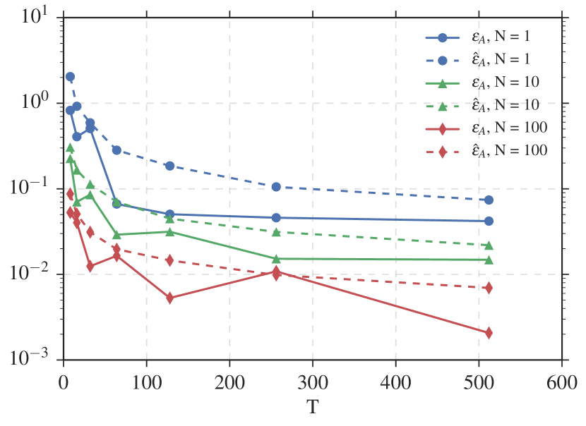
(a) Estimation Error in A𝐴A

Refer to caption

(b) Correctness of Bootstrap Estimate

Refer to caption

(c) Estimation Error in B𝐵B

Refer to caption

(d) Correctness of Bootstrap Estimate

Refer to caption

Figure 5: In these simulations: n=3𝑛3n=3, p=1𝑝1p=1, ρ=0.9𝜌0.9\rho=0.9, and M=2000𝑀2000M=2000. In (a), the spectral distances to A𝐴A (shown in the solid lines) are compared with the bootstrap estimates (shown in the dashed lines). In (b), the probability A𝐴A lies in BA^(ϵ^A)subscript𝐵^𝐴subscript^italic-ϵ𝐴B_{\widehat{A}}(\widehat{\epsilon}_{A}) estimated from 200020002000 trials. In (c), the spectral distances to Bsubscript𝐵B_{*} are compared with the bootstrap estimates. In (d), the probability B𝐵B lies in BB^(ϵ^B)subscript𝐵^𝐵subscript^italic-ϵ𝐵B_{\widehat{B}}(\widehat{\epsilon}_{B}) estimated from 200020002000 trials.
(a) Estimation Error in A𝐴A

Refer to caption

(b) Correctness of Bootstrap Estimate

Refer to caption

(c) Estimation Error in B𝐵B

Refer to caption

(d) Correctness of Bootstrap Estimate

Refer to caption

Figure 6: In these simulations: n=6𝑛6n=6, p=2𝑝2p=2, ρ=1.01𝜌1.01\rho=1.01, and M=2000𝑀2000M=2000. In (a), the spectral distances to A𝐴A are compared with the bootstrap estimates. In (b), the probability A𝐴A lies in BA^(ϵ^A)subscript𝐵^𝐴subscript^italic-ϵ𝐴B_{\widehat{A}}(\widehat{\epsilon}_{A}) estimated from 200020002000 trials. In (c), the spectral distances to B𝐵B are compared with the bootstrap estimates. In (d), the probability B𝐵B lies in BB^(ϵ^B)subscript𝐵^𝐵subscript^italic-ϵ𝐵B_{\widehat{B}}(\widehat{\epsilon}_{B}) estimated from 200020002000 trials.

Appendix G Experiments with Varying Rollout Lengths

Here we include results of experiments in which we fix the number of trials (N=6𝑁6N=6) and vary the rollout length. Figure 7 displays the estimation errors. The estimation errors on A𝐴A decrease more quickly than in the fixed rollout length case, consistent with the idea that longer rollouts of easily excitable systems allow for better identification due to higher signal to noise ratio. Figure 8 shows that stabilizing performance of the nominal is somewhat better than in the fixed rollout length case (Figure 2). This fact is likely related to the smaller errors on the estimation of A𝐴A (Figure 7).

(a) Least Squares Estimation Errors

Refer to caption

(b) Accuracy of Bootstrap Estimates

Refer to caption

Figure 7: The resulting errors from 100 identification experiments with with a total of N=6𝑁6N=6 rollouts is plotted against the length rollouts. In (a), the median of the least squares estimation errors decreases with T𝑇T. In (b), the ratio of the bootstrap estimates to the true estimates. Shaded regions display quartiles.
(a) LQR Cost Suboptimality

Refer to caption

(b) Frequency of Stabilization

Refer to caption

Figure 8: The performance of controllers synthesized on the results of the 100 identification experiments is plotted against the length of rollouts. In (a), the median suboptimality of nominal and robustly synthesized controllers are compared, with shaded regions displaying quartiles, which go off to infinity when stabilizing controllers are not frequently found. In (b), the frequency synthesis methods found stabilizing controllers.