Scale-dependent bias and bispectrum in neutrino separate universe simulations

Abstract

Cosmic background neutrinos have a large velocity dispersion, which causes the evolution of long-wavelength density perturbations to depend on scale. This scale-dependent growth leads to the well-known suppression in the linear theory matter power spectrum that is used to probe neutrino mass. In this paper, we study the impact of long-wavelength density perturbations on small-scale structure formation. By performing separate universe simulations where the long-wavelength mode is absorbed into the local expansion, we measure the responses of the cold dark matter (CDM) power spectrum and halo mass function, which correspond to the squeezed-limit bispectrum and halo bias. We find that the scale-dependent evolution of the long-wavelength modes causes these quantities to depend on scale and provide simple expressions to model them in terms of scale and the amount of massive neutrinos. Importantly, this scale-dependent bias reduces the suppression in the linear halo power spectrum due to massive neutrinos by 13 and 26% for objects of bias $\bar{b}=2$ and $\bar{b}\gg 1$, respectively. We demonstrate with high statistical significance that the scale-dependent halo bias cannot be modeled by the CDM and neutrino density transfer functions at the time when the halos are identified. This reinforces the importance of the temporal nonlocality of structure formation, especially when the growth is scale dependent.

I Introduction

Neutrinos are one of the most abundant particles in the universe, but are the least explored species in the Standard Model of particle physics. The solar Ahmad et al. (2002); Fukuda et al. (2002); Altmann et al. (2005); Abdurashitov et al. (2002) and atmospheric oscillation experiments Fukuda et al. (1998); Ashie et al. (2005); Sanchez et al. (2003) have revealed the two mass-squared differences, but the individual masses and their hierarchy are yet to be determined. Cosmological observables are primarily sensitive to the sum of neutrino masses hence offer a complementary probe of neutrinos. Thus, measuring the total neutrino mass is one of the most important goals of future CMB Henderson et al. (2016); Benson et al. (2014); Abazajian et al. (2016) and large-scale structure experiments Aghamousa et al. (2016); Ellis et al. (2014); Abate et al. (2012); Spergel et al. (2015); Laureijs et al. (2011).

The effect of massive neutrinos on cosmology is extensively studied (see e.g. Refs. Lesgourgues and Pastor (2006); Wong (2011) for reviews). At the background level, the expansion history changes due to the presence of neutrinos, and so the effect can, in principle, be probed by measuring the Hubble rate at various redshifts. At the growth level, due to the high velocity dispersion, massive neutrinos possess a free-streaming scale that acts as a Jeans scale below which they no longer cluster with the cold dark matter (CDM). As a result, the density perturbations become scale dependent, and the feature is imprinted on the matter power spectrum Hu and Eisenstein (1998); Eisenstein and Hu (1997) as well as the halo bias in the spherical collapse model LoVerde (2014a). While the effect at the linear order is well understood, the nonlinear nature of large-scale structure requires treatment beyond the leading order effect. In the mildly nonlinear regime one can tackle the problem using perturbative approaches Shoji and Komatsu (2010); Blas et al. (2014); Führer and Wong (2015); Dupuy and Bernardeau (2015); Archidiacono and Hannestad (2016); Levi and Vlah (2016); Inman and Pen (2017), but $N$-body simulations are still necessary to capture the fully nonlinear behavior, especially for accurately modeling the unprecedentedly precise data from future observations. Moreover, even in the linear regime, the biased tracers of large-scale structure such as galaxies and dark matter halos are themselves nonlinear objects.

The most straightforward way to include massive neutrinos in $N$-body simulations is to treat them as a different species of particles that have different mass than CDM particles Bird et al. (2012); Hannestad et al. (2012); Wagner et al. (2012); Villaescusa-Navarro et al. (2013, 2014); Castorina et al. (2014); Costanzi et al. (2013); Castorina et al. (2015). Due to the large thermal motion, however, massive neutrinos occupy the six-dimensional initial phase space (unlike CDM which occupy an effectively three dimensional initial subspace), one either needs many more particles for neutrinos than CDM to reduce the effect of Poisson shot noise or has to start simulations at later times and approximate the neutrinos as cold dark matter. There are many approaches put forward to bypass the difficulty. Refs. Agarwal and Feldman (2011); Heitmann et al. (2016) include the effect of massive neutrinos in the background evolution and initial conditions, but simulate only the dynamics of CDM+baryons. In Refs. Inman et al. (2015); Yu et al. (2016); Emberson et al. (2016), neutrinos are treated as a distinct species and injected into CDM simulations at later redshift. Hybrid approaches solve the coupled neutrino linear fluid equation Brandbyge and Hannestad (2010) or Boltzmann equation Ali-Haimoud and Bird (2012) with the nonlinear CDM evolution in $N$-body simulations. Recently, Ref. Banerjee and Dalal (2016) combined the particle and fluid descriptions to better estimate the properties of the thermal species and reduce the effect of shot noise.

In this paper, we present a complementary approach to modeling neutrinos in simulations, the separate universe (SU) approach. In the SU approach, a long-wavelength perturbation changes the expansion history locally, and the local observer would measure a different set of cosmological parameters compared to the background universe that does not have any long-wavelength perturbation. As a result, the small-scale structure formation in the SU would be influenced, or respond, accordingly. Applying this technique in $N$-body simulations, the response can be measured deep into the nonlinear regime where perturbation theory breaks down McDonald (2003); Sirko (2005); Gnedin et al. (2011); Li et al. (2014); Wagner et al. (2015a). Specifically, the SU simulations have enabled studies on the power spectrum covariance Li et al. (2014); Barreira and Schmidt (2017a), the squeezed-limit $n$-point function Wagner et al. (2015b); Barreira and Schmidt (2017b), the halo bias Li et al. (2016); Lazeyras et al. (2016); Baldauf et al. (2016), and the Lyman-$\alpha$ forest McDonald (2003); Cieplak and Slosar (2016); Chiang et al. (2017); Chiang and Slosar (2017). The only limitations for SU simulations in $\Lambda$CDM are the usual ones for any simulation: the resolution and the extent to which baryonic and astrophysical effects are modeled in the deeply nonlinear regime.

In the universe with CDM and massive neutrinos, the growth of density perturbations is scale dependent due to the free-streaming length of massive neutrinos. Thus, for SUs with scale-dependent density perturbations, the expansion histories are affected differently depending on the wavelengths, and so is the response of the small-scale structure formation. While it is nontrivial to find the corresponding densities and curvature of the Friedmann equation in the SUs with additional components that have Jeans scales Dai et al. (2015); Hu et al. (2016); Hu and Joyce (2017), it is easy to match the local Hubble expansion. Ref. Chiang et al. (2016) uses quintessence SU simulations to show that this approach provides excellent agreement between the power spectrum response and the position-dependent power spectrum (which is equivalent to the squeezed-limit bispectrum Chiang et al. (2014, 2015)) as well as the response and clustering biases in the sub-Jeans limit as long as the Jeans scale is much larger than the scales of interest. The goal of this paper is to generalize SU simulations for massive neutrinos to study the scale-dependent responses for long modes with different wavelengths where the free-streaming scale plays the role of the Jeans scale.

The rest of the paper is organized as follows. In Sec. II we construct SUs with massive neutrinos for different long-wavelength density perturbations and compute the responses of the linear growth. In Sec. III we implement the SU approach with massive neutrinos in $N$-body simulations. We present the results of the neutrino SU simulations in Sec. IV and Sec. V for power spectrum response and response bias, respectively. In Sec. VI we show how the linear halo power spectrum and the leading-order CDM squeezed-limit bispectrum are changed by the scale-dependent response. We discuss the results in Sec. VII. In App. A we demonstrate the choices of initial and horizon entry redshifts have minimum effects on solving the small-scale growth response. In App. B we derive the small-scale growths using the second-order Lagrangian perturbation theory with long-wavelength density perturbations in matter-radiation dominated universe. In App. C we discuss the two main caveats of neutrino SU simulations, that neutrino clustering is neglected within the simulations and that a separation of scales is assumed between the SU observables and the long-wavelength mode. In App. D we layout the detailed setup for numerically evaluating the spherical collapse in neutrino SU, which is compared against simulations in Sec. V. In App. E, we compare our predicted scale-dependent linear bias to $N$-body simulations that contain massive neutrino particles.

Throughout the paper, unless otherwise stated, we adopt a spatially flat $\nu\Lambda{\rm CDM}$ cosmology with a Hubble constant $h=0.7$, baryon density $\Omega_{b}=0.05$, CDM density $\Omega_{c}=0.25$, the CMB temperature $T_{\rm cmb}=2.725$ K, helium fraction $Y_{\rm He}=0.24$, and initial curvature power spectrum with the spectral index $n_{s}=0.95$ and amplitude which sets $\sigma_{8}=0.83$ today for the power spectrum of CDM+baryons. We assume a degenerate neutrino mass spectrum with each neutrino having $m_{\nu}=0.05~{}{\rm eV}$. This choice will produce a free-streaming scale consistent with that in the minimal mass normal and inverted hierarchies. For this scenario, the free-streaming scale is also still in the linear regime and the neutrino nonlinear clustering can be neglected (see App. C for detailed discussion). Depending on the number of massive neutrinos, $\Omega_{\Lambda}$ and the power spectrum normalization would change accordingly. We choose to fix $\Omega_{bc}=\Omega_{b}+\Omega_{c}$ since the particle mass of the simulation is given by $\Omega_{bc}$ (see Sec. III for more details), and to fix $\sigma_{8}$ since the nonlinear scale to the leading order is set by $\sigma_{8}$. In order to enhance the amplitude of the neutrinos effects so that they can be measured with a small set of simulations we shall study two cosmologies with $N_{\nu}=14$ and 28 massive neutrinos, which can be converted to $f_{\nu}$ by

$$f_{\nu}=\frac{\Omega_{\nu}}{\Omega_{bc}+\Omega_{\nu}}=\frac{N_{\nu}\frac{m_{\nu}}{93~{}{\rm eV}}}{\Omega_{bc}h^{2}+N_{\nu}\frac{m_{\nu}}{93~{}{\rm eV}}}\,,$$ (1)

and the corresponding values are 0.049 and 0.093, respectively. Finally, given our use of $N$-body techniques, in the following we will often refer to CDM+baryons as CDM.

II Neutrino separate universe

The construction of the SU with components other than CDM that possess Jeans scales has been studied extensively in Ref. Hu et al. (2016). Here we briefly summarize the expansion history of the SU in Sec. II.1, and focus on the discussion of the small-scale growth in the neutrino SU in Sec. II.2.

II.1 Expansion History

In the separate universe (SU) picture, an observer sitting in a long-wavelength density perturbation $\delta_{c}$ would measure the local mean density $\bar{\rho}_{cW}(a)$ as

$$\bar{\rho}_{cW}(a)=\bar{\rho}_{c}(a)\left[1+\delta_{c}(a)\right]\,,$$ (2)

where $\bar{\rho}_{c}$ is the global mean density, and the subscript $W$ denotes the windowed average across the scale much smaller than that of $\delta_{c}$. Note that the subscript $c$ denotes CDM+baryons under the assumption that baryons trace the CDM at large scales. While the SU picture does not require this assumption to be valid on small scales, in our $N$-body simulations we do combine them into a single CDM-like component. We therefore refer to this component as CDM in the following for simplicity. Since the total amount of CDM is conserved, this observer would find the local scale factor of the SU as

$$a_{W}=a\left[1+\delta_{c}(a)\right]^{-1/3}\approx a\left[1-\frac{1}{3}\delta_{c}(a)\right]\,,$$ (3)

which leads to the local Hubble expansion of the SU

$$H_{W}=\frac{\dot{a}_{W}}{a_{W}}=H-\frac{1}{3}\dot{\delta}_{c}=H\left(1-\frac{1}{3}\delta^{\prime}_{c}\right)\,,$$ (4)

with ${}^{\prime}\equiv d/d\ln a$. At early times

$$\lim_{a\to 0}\delta_{c}(a)\to 0\,,\quad\lim_{a\to 0}a_{W}\to a\,,\quad\lim_{a\to 0}H_{W}\to H\,,$$ (5)

and the physical conditions in local and global cosmology coincide. Notice that we implicitly assume that there is a universal time coordinate between the local SU and global universe, hence in the relativistic limit $\delta_{c}$ is the synchronous-gauge density perturbation Hu et al. (2016).

As we can see above, the construction of the SU only requires $\delta_{c}(a)$. While other components affect the evolution of $\delta_{c}(a)$, they do not enter explicitly into $a_{W}$. If these components influence the small-scale structure formation only through the local expansion, then the effect should be completely characterized by $\delta_{c}(a)$. The local scale factor $a_{W}$ does not even have to follow a Friedmann equation with the corresponding local densities and curvature which is only guaranteed above the Jeans scale Gnedin et al. (2011); Hu et al. (2016). Using quintessence as an example, it has been shown in Ref. Chiang et al. (2016) that the effect of the Jeans length on the small-scale observables can indeed be modeled accurately by $N$-body simulations with the SU expansion even below the Jeans scale where the SU technique might naively be supposed to fail.

In general $\delta_{c}(a)$ depends on wavelength, so $\delta_{c}(a)$ with different wavelengths would correspond to different SUs. Therefore, even if $\delta_{c}(a)$ of different wavelengths have the same value at the final time, their evolutionary histories are still distinct. This indicates the importance of the temporal nonlocality in structure formation. As a result, the response of the small-scale observable will become scale dependent, with the scale being the wavelength of the long mode. We shall demonstrate these scale-dependent responses in Sec. IV and Sec. V.

II.2 Small-scale linear growth

Massive neutrinos provide a perfect arena to explore the scale dependence of the response of the small-scale observables to the large-scale density perturbation. Due to their high velocity dispersion, neutrinos do not cluster with CDM on scales smaller than the free-streaming scale Lesgourgues and Pastor (2006)

$$k_{\rm fs}(z)=0.0287\frac{\sqrt{\Omega_{\Lambda}+\Omega_{m}(1+z)^{3}}}{(1+z)^{2}}~{}{\rm Mpc}^{-1}\,,$$ (6)

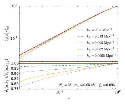
for our choice of $m_{\nu}$. Below this scale the fluctuations are washed out by free-streaming. As a result, the evolution of $\delta_{c}$ becomes scale dependent, and so does the corresponding SU. We use CLASS Blas et al. (2011); Lesgourgues and Tram (2011) to compute $\delta_{c}$ (including both CDM and baryons) as a function of the scale factor $a$ and the large-scale wavenumber $k_{L}$. Fig. 1 shows $\delta_{c}(a)/\delta_{c0}$ for different $k_{L}$ with $N_{\nu}=28$, where $\delta_{c0}=\delta_{c}(a=1)$. Modes with smaller $k_{L}$ grow faster than those of larger $k_{L}$ since neutrinos cluster with CDM on scales larger than the free-streaming scale, and the free-streaming scale decreases with time. With the evolution of $\delta_{c}(a)$, we can straightforwardly construct the SU expansion using Eqs. (3)–(4) for various $k_{L}$.

Figure 1: (Top) Evolution of $\delta_{c}(a)$, including both CDM and baryons, normalized to $\delta_{c0}=\delta_{c}(a=1)$ for different long-wavelengths $k_{L}$ with $N_{\nu}=28$. (Bottom) Ratios of $\delta_{c}(a)$ to that of $k_{L\downarrow}=5\times 10^{-2}~{}{\rm Mpc}^{-1}$.

Since in the SU approximation only CDM clusters, the small-scale linear growth in the SU, $D_{W}$, is given by

$$\frac{d^{2}D_{W}}{d\ln a_{W}^{2}}+\left(2+\frac{d\ln H_{W}}{d\ln a_{W}}\right)\frac{dD_{W}}{d\ln a_{W}}=\frac{3}{2}\frac{H_{0W}^{2}}{H_{W}^{2}}\frac{\Omega_{cW}}{a_{W}^{3}}D_{W}\,,$$ (7)

where $\Omega_{cW}H_{0W}^{2}=\Omega_{c}H_{0}^{2}$ is the background physical CDM energy density. Rewriting in terms of the global scale factor, we have

$$D^{\prime\prime}+\left(2+\frac{H^{\prime}}{H}\right)D^{\prime}-\frac{3}{2}\Omega_{c}(a)D=0\,,$$ (8)

$$\epsilon^{\prime\prime}+\left(2+\frac{H^{\prime}}{H}\right)\epsilon^{\prime}-\frac{3}{2}\Omega_{c}(a)\epsilon=\frac{2}{3}\delta_{c}^{\prime}D^{\prime}+\frac{3}{2}\Omega_{c}(a)\delta_{c}D\,,$$ (9)

where $D$ is the linear growth for sub-Jeans scale perturbations in the global universe, $\epsilon=D_{W}-D$ is the perturbation on $D$ due to $\delta_{c}$, and $\Omega_{c}(a)=(\Omega_{c}H_{0}^{2})/(H^{2}a^{3})$ is the CDM energy density in units of the critical energy density as a function of time. Note that the scale independence of both $D$ and $D_{W}$ is due to the SU approximation, since the full growth in cosmology with massive neutrinos is scale dependent. In other words, we only consider the growth with scale much smaller than the neutrino free-streaming scale ($k\gg k_{\rm fs}$), and in this limit it is scale independent. The challenge for solving Eq. (9) is to set up the initial condition for $\epsilon$. Specifically, as we have $f_{\nu}\gtrsim 0.05$ ($N_{\nu}=14$ and 28), at higher redshift massive neutrinos have even larger contribution to the total energy density compared to CDM, and so one cannot assume the SU being matter dominated to set up the initial condition of $\epsilon$.

Instead, let us consider setting up the initial condition at $a_{i}$ with $a_{\rm eq}\gg a_{i}$, and so the universe was radiation dominated and neutrinos were relativistic. During this epoch, $2+H^{\prime}/H\propto a_{i}/a_{\rm eq}\to 0$ and $\Omega_{c}(a)\propto a_{i}/a_{\rm eq}\to 0$, so the solution of the background growth is

$$D=C_{1}\ln\frac{a}{a_{H}}\,,$$ (10)

where $C_{1}$ and $a_{H}$ are integration constants. When solving the full perturbation equations from super to sub horizon $a_{H}$ is fixed to be approximately the scale factor at horizon-entry for the small-scale mode (see Ref. Hu and Sugiyama (1996) Eq. B12) and we have assumed $a_{i}\gg a_{H}$ in order to approximate these equations in Eq. (8) by dropping radiation clustering. Plugging Eq. (10) into Eq. (9), we require

$$\epsilon^{\prime\prime}=\frac{2}{3}\delta_{c}^{\prime}D^{\prime}=\frac{2}{3}C_{1}\delta_{c}^{\prime}$$ (11)

in the radiation-dominated universe. Assuming that the long-wavelength mode is super-horizon during this time, we also have $\delta_{c}\propto a^{2}$, which leads to

$$\epsilon=\frac{1}{3}C_{1}\delta_{c}+C_{2}+C_{3}\ln a\,,$$ (12)

where $C_{2}$ and $C_{3}$ are integration constants. As $\delta_{c}$ grows as $a^{2}$, the $C_{2}$ and $C_{3}$ terms should be negligible for any reasonable choice of parameters, and we only keep the $C_{1}$ term. Furthermore, $C_{1}$ is equivalent to an overall normalization which drops out once normalized to the final conditions, hence it is sufficient to describe the initial conditions as

$$D_{i}=\ln\frac{a_{i}}{a_{H}}\,,\quad\epsilon_{i}=\frac{1}{3}\delta_{c}(a_{i})D^{\prime}_{i}\,.$$ (13)

In App. A, we show that the results are insensitive to the choices of $a_{i}$ and $a_{H}$, hence we fix $a_{i}=10^{-6}$ and $a_{H}=10^{-10}$, which satisfies $a_{\rm eq}\gg a_{i}\gg a_{H}$.

Figure 2: Responses of the small-scale linear growth to the long-wavelength $\delta_{c}$ for different $k_{L}$ as a function of global scale factor for $N_{\nu}=28$. The horizontal dashed line represents the response in the matter-dominated SU, i.e. 13/21.

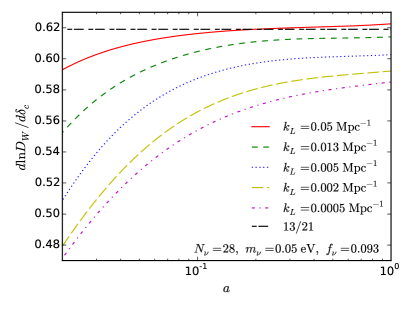
Fig. 2 shows the response of the linear growth for different $k_{L}$ as a function of the global scale factor for $N_{\nu}=28$. The horizontal dashed line represents the response in the matter-dominated SU, i.e. 13/21. As we can see, the smaller the $k_{L}$, the smaller the response. This is because on large scales neutrinos cluster with CDM, hence the SU is closer to the fiducial universe. We also find that in no case is the matter-dominated response appropriate since even at high redshift the radiation plays a role in the response which cannot be neglected when considering the effect of neutrinos.

III Separate universe simulations

To extend the treatment of the response of small-scale structure to the long-wavelength density perturbation into the nonlinear regime, we perform $N$-body simulations in SUs with different long-wavelength modes. Ref. Chiang et al. (2016) presented in detail the technique of running SU simulations with components other than CDM. In short, one first computes a table of $(a_{W},H_{W})$, passes it to the $N$-body code, and interpolates $H_{W}(a_{W})$ when necessary. Note that $H_{W}$ contains the energy density of the relativistic components, i.e. photons and neutrino.

The rest of the setup follows the standard procedure of SU simulations. Specifically, for constructing the initial conditions, we choose the initial power spectrum in the SU to be

$$P_{W}(k,a_{Wi})=P(k,a_{0})\left[\frac{D_{W}(a_{Wi})}{D(a_{0})}\right]^{2}\,,$$ (14)

where we set $a_{Wi}=0.02$ to be the initial scale factor of the SU and $a_{0}=1$ is the scale factor today in the global universe. Since CDM+baryons is the only component that clusters in SU approximation, we use the linear CDM+baryon transfer function from CLASS to calculate the linear power spectrum for the initial conditions, in cosmology with the corresponding numbers of massive neutrinos. To avoid confusion, in this paper we use units of comoving $[{\rm Mpc}^{-1}]$, and convert for code purposes as necessary. We then generate the initial conditions using realizations of Gaussian random fields for the primordial fluctuations, and evolve to $a_{Wi}$ using the second-order Lagrangian perturbation theory (2LPT) Crocce et al. (2006). In App. B, we derive the second-order growth under 2LPT with long-wavelength perturbations in matter-radiation dominated SUs, and the results are used to set up the initial conditions of SUs. The simulations are carried out by Gadget-2 Springel (2005) from $a_{Wi}$ to the final scale factor $a_{W0}=a_{0}(1-\delta_{c0}/3)$, corresponding to the same physical time as $a_{0}$.

We identify halos using the Amiga Halo Finder Gill et al. (2004); Knollmann and Knebe (2009), and use its dark energy feature to input the table of $(a_{W},H_{W},\Omega_{cW})$ in the corresponding SU. To account for the fact that in overdense and underdense SUs the thresholds for forming halos decrease and increase respectively, we set the density threshold in the SU to be

$$\Delta_{W}=\frac{\Delta}{1+\delta_{c}(a)}\approx\Delta\left[1-\delta_{c}(a)\right]\,,$$ (15)

with $\Delta=200$. We set the minimum number of particles for halos to be 100 for our halo catalogs, but to be conservative we only report the result with halos having more than 400 particles.

We run two sets of cosmologies, $N_{\nu}=14$ and 28 (corresponding to $f_{\nu}=0.049$ and 0.093), for the neutrino SU simulations. For both cosmologies we fix the box size $L$ and the number of particles $N_{p}^{3}$. Since the particle mass of the simulation is proportional to $\Omega_{bc}L^{3}/N_{p}^{3}$, fixing $\Omega_{bc}=0.3$ results in the identical mass resolution for the two $N_{\nu}$. We choose $L=700~{}{\rm Mpc}$, which is large enough so that the response in the linear regime can be obtained at $z=0$. Note that this box size is larger than the free-streaming scale of massive neutrinos of $0.05~{}{\rm eV}$, which is roughly $R_{\rm fs}=200~{}{\rm Mpc}$ today Lesgourgues and Pastor (2006). We set the number of particles to be $N_{p}^{3}=640^{3}$, hence the minimum halo mass we report in this paper is $2\times 10^{13}~{}M_{\odot}$.

For the long-wavelength perturbations, we set $\delta_{c0}=0$ and $\pm 0.01$. In order to sample the scale dependence of the response well, we run five different $k_{L}$ ($0.05-0.0005~{}{\rm Mpc}^{-1}$) for $N_{\nu}=28$; for $N_{\nu}=14$ we only run two limiting $k_{L}$ to quantify the dependence of the response on $N_{\nu}$, or equivalently $f_{\nu}$. For each choice of $N_{\nu}$ and $k_{L}$ we have $N_{s}=40$ sets of SU simulations for $\delta_{c0}=0,\pm 0.01$. To better quantify the scale dependence of the halo bias, which does not require simulations of $\delta_{c0}=0$ with our analysis method (see Sec. V.1 for detail), we additionally run 40 sets of SU simulations for $N_{\nu}=14$ and $28$ for $\delta_{c0}=\pm 0.01$. For each set of SU simulations (with or without $\delta_{c0}=0$), we adopt the same Gaussian realization so the cosmic variance largely cancels. The details of the neutrino SU simulations are summarized in Tab. 1. To simplify the notation, hereafter we denote $k_{L\uparrow}=0.0005~{}{\rm Mpc}^{-1}$ and $k_{L\downarrow}=0.05~{}{\rm Mpc}^{-1}$.

$N_{\nu}$	$\delta_{c0}$	$k_{L}\,[{\rm Mpc}^{-1}]$	$L\,{[{\rm Mpc}]}$​	$N_{p}$	$N_{s}$
14	0	$0.05,0.0005$	700	$640^{3}$	40
28	0	$0.05,0.013,0.005,0.002,0.0005$	700	$640^{3}$	40
14	$\pm 0.01$	$0.05,0.0005$	700	$640^{3}$	80
28	$\pm 0.01$	$0.05,0.013,0.005,0.002,0.0005$	700	$640^{3}$	80

Table 1: Summary of the neutrino SU simulations.

We point out that there are two main caveats in our neutrino SU simulations. First, within the SU, only CDM clusters, and the other components are smooth. Our simulation box, however, is larger than the neutrino free-streaming scale, so the neutrino clustering is missing on scales larger than the free-streaming scale of Eq. (6). Second, we assume that the wavelength of $\delta_{c}$ is much larger than the simulation box size, hence the curvature of $\delta_{c}$ is ignored. This is a good approximation when $k_{L}\ll\pi/L\approx 0.0045~{}{\rm Mpc}^{-1}$, but will be violated for larger $k_{L}$. In App. C, we discuss these two systematics in detail, and argue that neutrino clustering can be ignored for $k\gtrsim 0.05~{}{\rm Mpc}^{-1}$, while the corrections due to ignoring the curvature of $\delta_{c}$ are $\mathcal{O}(k_{L}^{2}R_{M}^{2})$ for halo bias with $R_{M}$ being the Lagrangian radius of halo with mass $M$ and $\mathcal{O}(k_{L}^{2}/k^{2})$ for power spectrum response with $k$ being the wavenumber of the small-scale power spectrum. For halo bias both systematics are negligible since the Lagrangian radii of halos of interest are $\lesssim 10~{}{\rm Mpc}$; for power spectrum response to avoid the systematics we only report results for $k\geq 0.05~{}{\rm Mpc}^{-1}$.

IV Power spectrum response

We now calibrate the response of the power spectrum to $\delta_{c}$ for different $N_{\nu}$ and $k_{L}$. In Sec. IV.1, we show the measurement of the power spectrum response in the neutrino SU simulations. In particular, we shall demonstrate with high statistical significance that the larger the scale of $k_{L}$, the smaller the power spectrum response until it is much larger than the neutrino free-streaming scale. In Sec. IV.2, we study the dependence of the growth response on $k_{L}$ and $N_{\nu}$.

IV.1 Growth response

In the presence of a long-wavelength $\delta_{c}$, the locally measured power spectrum differs from the global one. We can quantify the fractional difference between the local and global power spectra by

$$\frac{\Delta P}{P}\approx\frac{d\ln P}{d\delta_{c}}\delta_{c}\equiv R_{\rm tot}\delta_{c}\,,$$ (16)

where we define $R_{\rm tot}$ as the “response” of the local power spectrum to $\delta_{c}$. Refs. Barreira and Schmidt (2017b, a) provide a rigorous embedding of power spectrum response into the perturbative framework, and can be generalized to higher-oder responses. At leading order $R_{\rm tot}$ is independent of the amplitude of $\delta_{c}$, hence we can use the SU simulations with $\delta_{c0}=0,\pm 0.01$ to calibrate the response. This effect can also be measured in big $N$-body simulations by the bispectrum in the squeezed limit with the angle average of the cosine between the long and short modes (see e.g. Ref. Chiang et al. (2014))

$$\lim_{k_{L}\to 0}B(k,k^{\prime},k_{L})\equiv B^{\rm sq}(k,k_{L})=R_{\rm tot}P(k_{L})P(k)\,,$$ (17)

where $k_{L}$ corresponds to the mode of $\delta_{c}$ and $k\approx k^{\prime}$ corresponds to the mode of $P$ averaged over direction. Note that unless otherwise stated, we denote the CDM+baryon power spectrum and bispectrum without subscript for compactness.

In the $\Lambda$CDM cosmology, the evolution of $\delta_{c}$ is independent of the wavenumber of the large-scale mode $k_{L}$, and so as $R_{\rm tot}$. As a result, $R_{\rm tot}$ depends only on time and the small-scale wavenumber $k$. If the universe, however, has additional components that cluster and remain smooth above and below Jeans scales, such as quintessence or massive neutrinos, then both $\delta_{c}$ and $R_{\rm tot}$ would depend on $k_{L}$ (see Ref. Chiang et al. (2016) for the scale-dependent response in quintessence SU). Therefore, $R_{\rm tot}=R_{\rm tot}(k,k_{L},a)$. This also indicates that the reduced squeezed-limit bispectrum would depend on $k_{L}$.

Figure 3: Growth response measured from 40 sets of neutrino separate universe simulations as a function of small-scale $k$ for different large-scale $k_{L}$ (denoted by various colors). The top and bottom panels show $N_{\nu}=14$ and 28 ($f_{\nu}=0.049$ and 0.093), and the left and right panels show $z=3$ and 1. The lines with shaded areas show the measurement from simulations with the error on the mean, whereas the lines without shaded areas show the analytic calculation with the 1-loop power spectrum response (see the text for details).

Physically, the total response can be separated into three pieces Li et al. (2014):

$$R_{\rm tot}=R_{\rm growth}+R_{\rm dilation}+R_{\bar{\rho}}\,.$$ (18)

$R_{\rm growth}$ specifies the change due to the growth of the small-scale density fluctuation between the separate and global universes at a fixed comoving $k$; $R_{\rm dilation}$ describes the change of comoving $k$ between separate and global universes due to different expansion histories; $R_{\bar{\rho}}$ accounts for the different mean densities in separate and global universes used to define the small-scale density fluctuation. Note that $R_{\rm dilation}$ and $R_{\bar{\rho}}$ are nondynamical effects and can be computed without additional simulations, as we shall discuss in detail in Sec. VI. On the other hand, the growth response is dynamical and so requires $N$-body simulations for an accurate estimate.

In order to measure the growth response from SU simulations, we distribute the dark matter particles onto a $640^{3}$ grid using the cloud-in-cell density assignment to construct the density fluctuation, and Fourier transform the fluctuation with FFTW fft to estimate the power spectrum $\hat{P}(k,a)$. We then estimate the growth response by

$$\hat{R}_{\rm growth}(k,k_{L},a)\equiv\frac{\hat{P}(k,a|\delta_{c0}^{+}(k_{L}))-\hat{P}(k,a|\delta_{c0}^{-}(k_{L}))}{2\hat{P}(k,a|\delta_{c0}^{0})\delta_{c}(k_{L},a)}\,,$$ (19)

where $\delta_{c0}^{0,\pm}=0$, $\pm 0.01$.

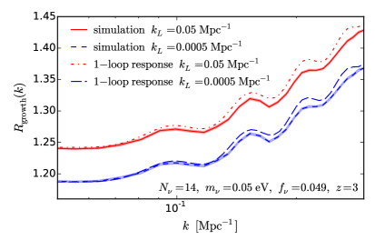
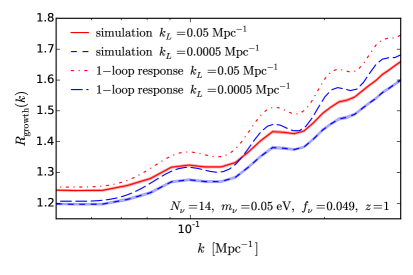
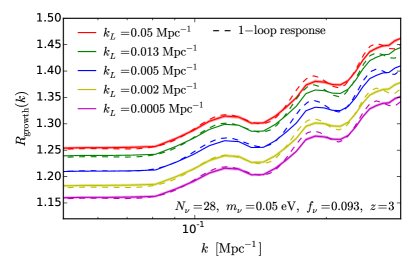
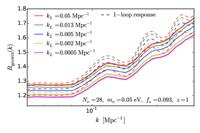
The lines with shaded areas in Fig. 3 show the mean of the growth response measured from neutrino SU simulations as a function of small-scale $k$ for different large-scale $k_{L}$ (denoted by various colors), and the shaded areas represent the error on the mean. The top and bottom panels show $N_{\nu}=14$ and 28, and the left and right panels show $z=3$ and 1. We show the results at higher redshifts and on larger scales ($k\leq 0.3~{}{\rm Mpc}^{-1}$) because it is the regime in which the 1-loop calculation has the predicting power, which will be discussed in the following. We find with high statistical significance that the growth response indeed depends on the large-scale wavenumber $k_{L}$ for all redshifts and small scales. Note especially that for $k\gtrsim 0.1~{}{\rm Mpc}^{-1}$, where the systematics due to small-scale neutrino clustering and the curvature of the long-wavelength mode can be ignored, the dependence of $R_{\rm growth}$ on $k_{L}$ persists and is similar in amplitude.

To better understand the measurement from neutrino SU simulations quantitatively, we compute the growth response using perturbation theory. Specifically, in perturbation theory the growth response can be modeled as

$$R_{\rm growth}(k,k_{L},a)=\frac{d\ln P(k,a)}{d\ln D_{W}(a)}\left[\frac{d\ln D_{W}}{d\delta_{c}}(k_{L},a)\right]\,,$$ (20)

where the second term in the right-hand side is computed in Fig. 2. Note that in Eq. (20) the dependencies on $k$ and $k_{L}$ are separated into the first and second terms in the right-hand side. In the linear regime, $P\approx P_{\rm lin}$ is proportional to $D_{W}^{2}$ and so

$$\frac{d\ln P_{\rm lin}(k,a)}{d\ln D_{W}(a)}=2\,.$$ (21)

In the mildly nonlinear regime, we utilize the 1-loop power spectrum in the standard perturbation theory (see e.g. Ref. Jeong and Komatsu (2006)): $P_{\rm 1-loop}=P_{\rm lin}+P_{22}+2P_{13}$, where $P_{22}$ and $P_{13}$ are the nonlinear correction and proportional to $D_{W}^{4}$ if $\Omega_{cW}(a_{W})/f_{W}^{2}(a_{W})\approx 1$. As a result,

$$\frac{d\ln P_{\rm 1-loop}(k,a)}{d\ln D_{W}(a)}=2\left[1+\frac{P_{22}(k,a)+2P_{13}(k,a)}{P_{\rm 1-loop}(k,a)}\right]\,.$$ (22)

The lines without shaded areas in Fig. 3 show the growth response computed from the 1-loop power spectrum using Eq. (22) and Fig. 2. On large scale, the nonlinear correction becomes subdominant, and the 1-loop calculation approaches to the linear prediction and becomes $k$ independent. We find that the 1-loop calculation is generally in good agreement with the measurement, especially at $z=3$, as would be expected and hence validates the SU simulations. On smaller scales and at lower redshift, the nonlinearities are too large to be modeled by the perturbation theory, hence we find a more significant difference.

IV.2 Dependence on $k_{L}$ and $N_{\nu}$

We have shown in Fig. 3 that the small-scale growth responds differently to $\delta_{c}$ with various $k_{L}$. To better study this feature, let us define the “growth response step” as the ratio of the growth response with respect to that of $k_{L\uparrow}=0.0005~{}{\rm Mpc}^{-1}$, i.e.

$$R_{\rm growth}(k,k_{L},N_{\nu},a)/R_{\rm growth}(k,k_{L\uparrow},N_{\nu},a)\,.$$ (23)

We first examine the dependence of the step on the small-scale $k$ by fixing $N_{\nu}$ and $k_{L}$, and we find that it is fairly independent of $k$. More precisely, at $z=0$ the step between $k_{L\uparrow}$ and $k_{L\downarrow}=0.05~{}{\rm Mpc}^{-1}$ departs from a scale-independent constant at the 10% level for $k\lesssim 0.6~{}{\rm Mpc}^{-1}$. This is not surprising: in Fig. 3 $R_{\rm growth}$ of different $k_{L}$ have similar scale dependence in $k$. Thus, in the following we fix $k=0.252~{}{\rm Mpc}^{-1}$ to avoid the systematics from neutrino clustering as well as the curvature of $\delta_{c}$, and focus on the dependencies of $k_{L}$ and the number of massive neutrinos $N_{\nu}$.

Figure 4: Growth response step at $z=1$ (left) and 0 (right) for $N_{\nu}=28$ as a function of the large-scale mode $k_{L}$. The blue data points show the measurement from SU simulations with the small-scale mode $k=0.252~{}{\rm Mpc}^{-1}$, whereas the red solid line shows the numerical calculation of $d\ln D_{W}/d\delta_{c}$ normalized at $k_{L\uparrow}=0.0005~{}{\rm Mpc}^{-1}$. The error bars show the error on the mean.

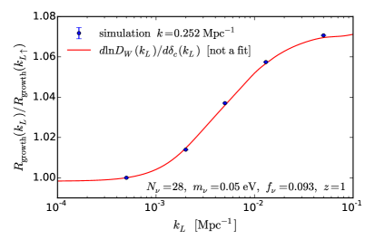
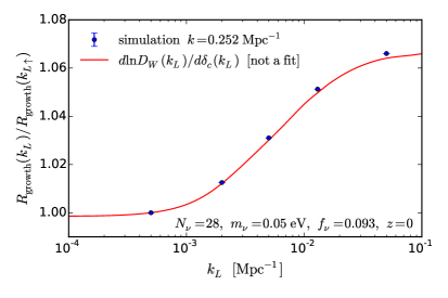
Fig. 4 shows the growth response step for $N_{\nu}=28$ as a function of $k_{L}$. The blue data points with error bars show the measurement of the step from neutrino SU simulations at $z=1$ (left) and 0 (right). Note that by definition the error bars of the step are zero at $k_{L\uparrow}$. For the other $k_{L}$, the small error bars are the outcome of the highly correlated growth responses, since we use the same random realizations for different $k_{L}$. We find that the dependence of the growth response step on $k_{L}$ is statistically significant, indicating that the growth response is indeed affected by the temporal evolution of $\delta_{c}$.

Given the independence of the step on the small-scale $k$ and the good agreement with perturbation theory for linear $k$ demonstrated in the previous section, the response of the linear growth function should provide an accurate calibration of its shape and amplitude. We follow the procedures in Sec. II.2 to numerically compute $d\ln D_{W}/d\delta_{c}$ with $N_{\nu}=28$ for various $k_{L}$, and normalize it at $k_{L\uparrow}$. The result is shown as the red solid line in Fig. 4, and we find it is in excellent agreement with the measurement. Notice that the red line is slightly less than unity on large scale, because we normalize the step at $k_{L\uparrow}$. Should we normalize the step feature with a smaller $k_{L}$, the red line would approach to unity on large scale.

Figure 5: Growth response step between $k_{L\uparrow}=0.0005~{}{\rm Mpc}^{-1}$ and $k_{L\downarrow}=0.05~{}{\rm Mpc}^{-1}$ at $z=1$ (left) and 0 (right) as a function of the number of massive neutrinos $N_{\nu}$, with the corresponding $f_{\nu}$ labeled on the top $x$-axis. The blue data points show the measurement from SU simulations with the small-scale mode $k=0.252~{}{\rm Mpc}^{-1}$; the red solid line shows the numerical calculation of $d\ln D_{W}/d\delta_{c}$ normalized at $k_{L\uparrow}$; the green dashed line shows the linear relation of the two data points. The error bars show the error on the mean.

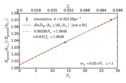
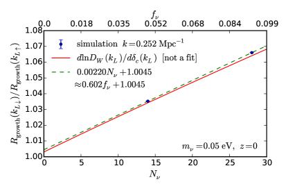
We next examine the growth response step between $k_{L\uparrow}$ and $k_{L\downarrow}$ as a function of $N_{\nu}$, i.e. $R_{\rm growth}(k_{L\downarrow},N_{\nu})/R_{\rm growth}(k_{L\uparrow},N_{\nu})$. The blue data points in Fig. 5 show the measurement from neutrino SU simulations at $z=1$ (left) and 0 (right), with the corresponding $f_{\nu}$ labeled on the top $x$-axis. It is evident that the growth response step is non-zero, and the larger the $N_{\nu}$ the larger the step size. Assuming that the measured growth response step is linear in $N_{\nu}$, we can solve the slope and the intercept, and the result is shown as the green dashed line, with the values given in the legend. To convert $N_{\nu}$ to the commonly used $f_{\nu}$, we use Eq. (1) and take the limit that $f_{\nu}\ll 1$, which leads to $N_{\nu}\approx 274f_{\nu}$. We find that the slope of the measured growth response step for artificially large $N_{\nu}$ in terms of $f_{\nu}$ is approximately 0.6. Interestingly the best fit does not go to unity at $N_{\nu}=0$ though this value is far from the simulated values.

To avoid extrapolation from the simulated values of $N_{\nu}$, we can also model the growth response step by numerically evaluating $d\ln D_{W}/d\delta_{c}$ at $k_{L\uparrow}$ and $k_{L\downarrow}$ as a function of $N_{\nu}$. Note that we only vary the number of massive neutrinos, not their mass, and correspondingly do not include massless neutrinos when $N_{\nu}<3$. The result is shown as the red solid line in Fig. 5, which is in good agreement with the measurement. If we solve the slope $A$ in terms of $f_{\nu}$ and intercept $(1+B)$ for the red solid line in the limit that $f_{\nu}\ll 1$, then we get $A=0.68,0.63$ and $B=0.0048,0.0030$ for $z=1,0$.

In this model we can interpret the non-zero $B$ intercept of the step in the $N_{\nu}=0$ limit as due to photons. Photons possess a Jeans scale of the sound horizon before recombination and the horizon after and cause their own growth response. If the calculation is done in the universe without photons, then the growth response step would go to unity at $N_{\nu}=0$, since the growth of the long-wavelength modes in $\Lambda$CDM cosmology is scale independent. Note also that these values are obtained assuming $m_{\nu}=0.05~{}{\rm eV}$ with the change in $f_{\nu}$ coming from the number of massive neutrinos. For a different neutrino mass, we expect the growth response step between the super- and sub-Jeans limits can still be approximated by the same slope, but the scale of the transition in $k_{L}$ would shift due to the a different free-streaming scale.

V Scale-Dependent Bias

Let us now turn to the response of the halo mass function, which determines the relationship between the number density of halos and the long-wavelength density fluctuation $\delta_{c}$, i.e. the linear density bias of halos. In Sec. V.1, we discuss the analysis of the response bias from SU simulations. In Sec. V.2, we present the response bias from the neutrino SU simulations, and study its dependence on $k_{L}$ and $N_{\nu}$. As in the previous section, we shall demonstrate with high statistical significance that the response bias is scale dependent due to the presence of the neutrino free-streaming scale. In Sec. V.3, we compare the response bias with different bias models and discuss the importance of temporal nonlocality in producing scale-dependent bias.

V.1 Response bias

The linear bias of halos can be regarded as the linear response of the halo abundance of mass $M$ to the long-wavelength density perturbation, i.e.

$$b(M)\equiv\frac{d\delta_{h}(M)}{d\delta_{c}}=\frac{d\ln n_{\ln M}(M)}{d\delta_{c}}\,,$$ (24)

where $n_{\ln M}(M)=-dn(M)/d\ln M$ is the differential halo mass function and $n(M)$ is the cumulative halo mass function. We refer to this as “response bias”. Physically, the enhanced growth in a SU with $\delta_{c}>0$ makes massive halos more abundant compared to their counterparts with $\delta_{c}<0$, making their number density fluctuation a biased tracer of $\delta_{c}$. Therefore, by measuring how the halo mass function is affected by $\delta_{c}$ in SU simulations, we have a direct calibration of the halo bias without the standard clustering measurement Li et al. (2016); Lazeyras et al. (2016); Baldauf et al. (2016).

While we do not write it explicitly in Eq. (24), $\delta_{c}$ is a function of the wavenumber of the long mode $k_{L}$ when its growth depends on scale. For example, if there are additional components that possess Jeans scales, such as quintessence, then the growth becomes scale dependent and so $b(M)$ would depend on $k_{L}$ contrary to the expectations of purely spatial and temporally local bias Chiang et al. (2016). The SU simulations thus allow us to study the scale-dependent bias due to the free-streaming length of massive neutrinos LoVerde (2014a).

The most straightforward way of measuring the response of the halo mass function is to bin the halo abundance in halo mass and compare it for different $\delta_{c}$. This, however, is inefficient since we can only measure the effect if the change in halo mass moves it across the mass bins. Instead, we adopt the abundance matching technique introduced in Ref. Li et al. (2016) to characterize the response bias. Specifically, for each set of $\delta_{c0}=\pm 0.01$ SU simulation we first bootstrap resample the total 80 realizations and combine the halo catalogs sorted in mass. We then measure the discrete threshold mass shift by

$$s_{i}(\ln M_{i})=\frac{\ln M_{i}^{+}-\ln M_{i}^{-}}{2|\delta_{c}|}\,,$$ (25)

where $M_{i}^{\pm}$ are the masses of the $i^{\rm th}$ most massive halo in the $\delta_{c0}=\pm 0.01$ SU sample and $M_{i}=(M_{i}^{+}M_{i}^{-})^{1/2}$. Next we use a smoothing spline function with two knots per dex in halo mass to estimate the continuous threshold mass shift $\hat{s}(\ln M)$ as well as the cumulative halo mass function $\hat{n}(\ln M)$ using all $M_{i}$ entry by entry. The derivative of the smooth cumulative mass function fit gives the differential mass function $\hat{n}_{\ln M}=-d\hat{n}/d\ln M$. The cumulative Lagrangian bias of halos with mass greater than threshold mass $M$, denoted with an overbar, can thus be estimated as

$$\hat{\bar{b}}^{L}(M)=\frac{\hat{n}_{\ln M}(\ln M)\hat{s}(\ln M)}{\hat{n}(\ln M)}\,.$$ (26)

Eq. (26) measures the Lagrangian bias since the SU simulations are performed with the same comoving instead of physical volume, and we obtain the cumulative Eulerian bias by transforming from Lagrangian to Eulerian coordinates:

$$\hat{\bar{b}}(M)=1+\hat{\bar{b}}^{L}(M)\,.$$ (27)

Finally, repeating the procedure with different resamplings for 8,000 times, we have an estimate of the error on the mean.

V.2 Scale dependence

Figure 6: Lagrangian response bias measured from 80 sets of neutrino separate universe simulations as a function of halo mass. The top and bottom panels show $N_{\nu}=14$ and 28 ($f_{\nu}=0.049$ and 0.093); the left and right panels show $z=1$ and 0. In each panel, the top plot shows the response bias $\bar{b}^{L}(M)$, and the bottom plot shows the ratios of the biases with respect to $k_{L\uparrow}=0.0005~{}{\rm Mpc}^{-1}$, i.e. $\bar{b}^{L}(k_{L})/\bar{b}^{L}(k_{L\uparrow})$. The lines and shaded region show the smoothed estimate and the bootstrap error on the mean.

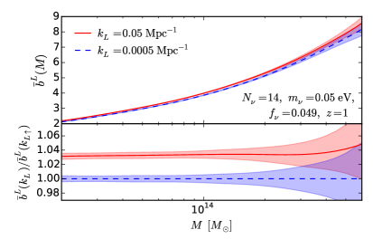
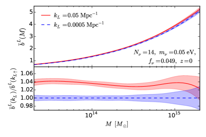
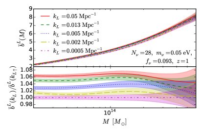
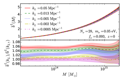
The response bias as measured from the SU simulations shows a statistically significant scale dependence where the bias increases with $k_{L}$ and $N_{\nu}$ in a manner nearly independent of halo mass. Fig. 6 shows the Lagrangian response bias measured from the 80 sets of neutrino SU simulations as a function of halo mass. The top and bottom panels show $N_{\nu}=14$ and 28, whereas the left and right panels show $z=1$ and 0. In each panel the top and bottom plots show the response bias $\bar{b}^{L}(M)$ and the ratio $\bar{b}^{L}(k_{L})/\bar{b}^{L}(k_{L\uparrow})$. The lines and shaded region show the smoothed estimate and the bootstrap error. We find that for a fixed $N_{\nu}$, the response bias systematically increases with $k_{L}$, apparent especially for $N_{\nu}=28$ where the five values of $k_{L}$ more fully map out a larger net effect, indicating that $\bar{b}^{L}$ is indeed scale dependent.

The scale dependence increases with $N_{\nu}$ and does not evolve much between $z=1$ and 0 or with mass, although the uncertainty increases at the high-mass end due to rarity of such objects. Note that the mild oscillations in the ratio for $N_{\nu}=14$ at $z=0$ are still statistically consistent with being independent of halo mass due to the correlations inherent in our estimation technique.

Figure 7: Lagrangian response bias step at $z=1$ (left) and 0 (right) for $N_{\nu}=28$ ($f_{\nu}=0.093$) as a function of the large-scale mode $k_{L}$. Different colored symbols represent halo catalogs of different masses, with the error bars showing the bootstrap error on the mean. The black dashed and magenta dot-dashed lines show the modeling from spherical collapse ($\bar{b}_{S}^{L}$) and universal mass function ($\bar{b}_{D}^{L}$) bias models (see detailed discussion in Sec. V.3).

Figure 8: Lagrangian response bias step between $k_{L\uparrow}=0.0005~{}{\rm Mpc}^{-1}$ and $k_{L\downarrow}=0.05~{}{\rm Mpc}^{-1}$ at $z=1$ (left) and 0 (right) as a function of the number of massive neutrinos $N_{\nu}$, with the corresponding $f_{\nu}$ labeled on the top $x$-axis. Different colored symbols represent halo catalogs of different masses, and the error bars show the bootstrap error on the mean. The cyan dotted line is a fit to all the colored symbols with the slope and the intercept shown in the legend, which provides a rough estimate of the magnitude of the effect. The black dashed and magenta dot-dashed lines show the predictions from spherical collapse ($\bar{b}_{S}^{L}$) and universal mass function ($\bar{b}_{D}^{L}$) bias models (see detailed discussion in Sec. V.3).

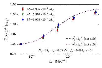
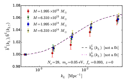
In order to quantify the scale dependence of bias further, we first isolate the scale dependence by taking the ratio with respect to the smallest wavenumber in the simulations $k_{L\uparrow}=0.0005~{}{\rm Mpc}^{-1}$, i.e.

$$\bar{b}^{L}(M,k_{L},N_{\nu},a)/\bar{b}^{L}(M,k_{L\uparrow},N_{\nu},a)\,,$$ (28)

for various choices of $M$. The uncertainty in this ratio becomes large for high-mass halos, again due to their rarity, and for low-mass halos, likely due to the inability of mass ordering to identifying the “same” halos in the $\delta_{c0}=\pm 0.01$ SU halo catalogs due to mergers and accretion. For these reasons we take $M=2\times 10^{13}$, $6.3\times 10^{13}$, and $2\times 10^{14}~{}M_{\odot}$ at $z=1$, and the same for $z=0$ with the addition of $6.3\times 10^{14}~{}M_{\odot}$. Note that since we measure the cumulative bias, $\bar{b}^{L}(M)$ of different masses are correlated.

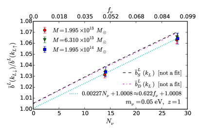
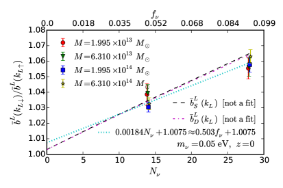
The colored symbols in Fig. 7 show the response bias step for $N_{\nu}=28$ as a function of the long mode $k_{L}$ for halos with different masses. The uncertainty on the response bias is larger than that of the growth response, but a similar step-like feature is still evident. Note that the error bar is for the ratio with respect to $k_{L\uparrow}$, so by definition the uncertainly is zero at $k_{L\uparrow}$. This step feature is at most weakly dependent on mass, but the dependence can also be a consequence of the estimation technique, i.e. the mild oscillations of the ratio of the response bias shown in Fig. 6.

We next examine the $N_{\nu}$ dependence of the full amplitude of the step, as quantified by the bias ratio between the largest and smallest wavenumbers i.e. $\bar{b}^{L}(k_{L\downarrow},N_{\nu})/\bar{b}^{L}(k_{L\uparrow},N_{\nu})$, and the result is shown in Fig. 8. The results are consistent with a linear dependence on $N_{\nu}$ that is weakly dependent on mass. To guide the eye, we fit all the data points in Fig. 8 to a linear relation. Note that this is not strictly correct due to the correlation of the cumulative biases of halos with different mass cuts, but it suffices for a rough estimation. The cyan dotted line in Fig. 8 shows the fit from all the colored symbols, with the slope and intercept shown in the legend. Note that as in the power spectrum response, the intercept at $N_{\nu}=0$ needs not vanish since the photons can also produce scale-dependent bias. We shall discuss the interpretation of these results next.

V.3 Bias models

The behavior of scale-dependent bias uncovered in the SU simulations above both illuminate the assumptions behind, and are illuminated by the predictions of, various bias models. Here we consider how three types of models commonly found in the literature can be extended to accommodate scale-dependent bias: spherical collapse, universal mass function, and scale-free linear bias with respect to multiple tracers. We call these $\bar{b}_{S}^{L}$, $\bar{b}_{D}^{L}$, and $\bar{b}_{T}$ respectively.

Scale-dependent spherical collapse bias is based on calculating the effect of $\delta_{c}$ on the collapse of a spherical tophat overdensity in the SU and we implement it here by assuming that the collapse depends on the CDM alone. Specifically, the Lagrangian bias with respect to CDM is given by

$$\bar{b}^{L}_{S}(M,k_{L})=\frac{d\ln n(M)}{d\delta_{c}}=\frac{d\ln n(M)}{d\delta_{\rm crit}}\frac{d\delta_{\rm crit}}{d\delta_{c}}(k_{L})\,,$$ (29)

where $\delta_{\rm crit}$ is the linearly extrapolated density threshold for collapse and $d\ln n/d\delta_{\rm crit}$ depends only on the halo mass. In the presence of massive neutrinos, the response of $\delta_{\rm crit}$ with respect to $\delta_{c}$ becomes scale dependent LoVerde (2014b, a), and the scale dependence of the halo bias is entirely characterized by $d\delta_{\rm crit}/d\delta_{c}$. In App. D we outline in detail the setup for numerically evaluating $d\delta_{\rm crit}/d\delta_{c}$. The resulting prediction for the step in the Lagrangian bias

$$\frac{\bar{b}^{L}_{S}(M,k_{L})}{\bar{b}^{L}_{S}(M,k_{L\uparrow})}=\frac{\left[d\delta_{\rm crit}/d\delta_{c}\right](k_{L})}{\left[d\delta_{\rm crit}/d\delta_{c}\right](k_{L\uparrow})}\,,$$ (30)

is shown as the black dashed line in Fig. 7. Note that with no free parameters, the spherical collapse model captures the main trends of scale-dependent bias quite well. In particular this model predicts that the scale dependence of the bias is independent of halo mass and helps explain the weak dependence seen in the SU simulations.

Another simple model of bias which we call the universal mass function bias, $\bar{b}_{D}^{L}$, comes from assuming that the mass function is a universal functional of the power spectrum. In the SU picture, this should be the local power spectrum $P_{W}$ so that

$$\bar{b}_{D}^{L}(M,k_{L})=\frac{d\ln n(M;P_{W})}{d\delta_{c}}(k_{L})\propto\frac{d\ln D_{W}}{d\delta_{c}}(k_{L})\,,$$ (31)

where the mass-dependent proportionality approximately holds regardless of whether $P_{W}$ is considered to be the linear or nonlinear power spectrum as shown in Sec. IV. Like the spherical collapse model, the step of $\bar{b}_{D}^{L}$ does not contain free parameters, i.e.

$$\frac{\bar{b}_{D}^{L}(M,k_{L})}{\bar{b}_{D}^{L}(M,k_{L\uparrow})}=\frac{\left[d\ln D_{W}/d\delta_{c}\right](k_{L})}{\left[d\ln D_{W}/d\delta_{c}\right](k_{L\uparrow})}\,.$$ (32)

In this model, the scale dependence of bias is directly inherited from the scale dependence of the power spectrum response, which itself is a proxy for the response of small-scale structure responsible for halo formation. It therefore plays a role similar to $\delta_{\rm crit}$ in the spherical collapse model and indeed we find in Fig. 7 that the growth response (magenta dot-dashed line) and spherical collapse predictions are similar

$$\frac{d\ln D_{W}}{d\delta_{c}}(k_{L})\approx\frac{d\delta_{\rm crit}}{d\delta_{c}}(k_{L})\,,$$ (33)

and describe the SU simulations results equally well.

Figure 9: Comparison of the best-fit transfer function bias model (dashed lines; see the text for detailed description of the model) at $z=1$ (left) and 0 (right) to the measured Lagrangian response bias step from neutrino separate universe simulations as in Fig. 6. Note that the data points of a given mass are highly correlated in $k_{L}$ due to the same random realizations used in separate universe simulations which forbids the large change in slope that would be required to move the curves towards the central points. See Fig. 10, which displays the same fitting result with less correlation by taking the difference of neighboring data points, for a better visual representation.

The third type is based on the assumption that bias is temporally and spatially local, and hence scale free, but that halos can be biased with respect to multiple species of matter separately, in this case CDM and neutrinos $\delta_{h}=b_{c}\delta_{c}+b_{\nu}\delta_{\nu}$. Therefore, the Eulerian bias with respect to CDM, i.e. $\delta_{h}(M,k_{L})=\bar{b}_{T}(M,k_{L})\delta_{c}(k_{L})$, can be written as

$$\bar{b}_{T}(M,k_{L})=b_{c}(M)+b_{\nu}(M)\frac{T_{\nu}(k_{L})}{T_{c}(k_{L})}\,,$$ (34)

where $b_{c}$ and $b_{\nu}$ are bias parameters depending on halo mass, and the scale dependence is encoded in the neutrino and CDM+baryon transfer functions, which are computed using CLASS. To compare with the step of the Lagrangian bias, the transfer function bias can be written as

$$\frac{\bar{b}_{T}(M,k_{L})-1}{\bar{b}_{T}(M,k_{L\uparrow})-1}=\frac{\tilde{b}_{c}+T_{\nu}(k_{L})/T_{c}(k_{L})}{\tilde{b}_{c}+T_{\nu}(k_{L\uparrow})/T_{c}(k_{L\uparrow})}\,,$$ (35)

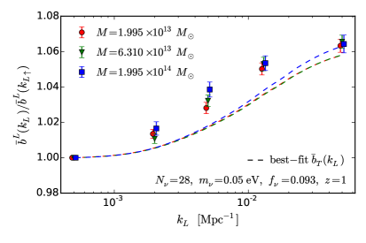
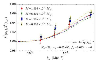
where $\tilde{b}_{c}=(b_{c}-1)/b_{\nu}$. Therefore, the step of the transfer function bias model has one fitting parameter $\tilde{b}_{c}$ which controls the amplitude of the scale dependence but crucially the shape cannot be adjusted. The $\bar{b}_{T}$ model with the best-fit $\tilde{b}_{c}$ is shown in Fig. 9 and is a poor fit to the simulations especially at $z=1$. Note that despite having an adjustable amplitude parameter the best fit systematically undershoots the step results because of their strong constraint on the shape of the step. The large correlation in the data points means that the slope of the step is much better constrained than $\chi$-by-eye would suggest.

To obtain a better visual representation of the problem, we take the the difference of the Lagrangian response bias step between neighboring points, i.e. $\left[\bar{b}^{L}(k_{L,i})-\bar{b}^{L}(k_{L,i-1})\right]/\bar{b}^{L}(k_{L\uparrow})$, where $i=0\cdots 4$ corresponds to $k_{L,i}=0.0005$, 0.002, 0.005, 0.013, and $0.05~{}{\rm Mpc}^{-1}$. This largely reduces the correlation between data points (the typical absolute values of the correlation drops from 0.6 to 0.2), while keeping the fitting unchanged. The top panel in Fig. 10 shows the comparison at $z=1$ (left) and 0 (right) between the measurement and the $\bar{b}_{T}(k_{L})$ model, and the bottom panel shows the comparison with the $\bar{b}_{S}^{L}(k_{L})$ and $\bar{b}_{D}^{L}(k_{L})$ models. We can see that the problem with $\bar{b}_{T}$ is that the slope monotonically rises with $k_{L}$ whereas the data prefer a decline by the highest point for most masses and redshifts. This problem does not occur for $\bar{b}_{S}^{L}$ and $\bar{b}_{D}^{L}$ which have the right shape for the scale dependence.

Figure 10: Difference of the Lagrangian response bias step between neighboring points, i.e. $\left[\bar{b}^{L}(k_{L,i})-\bar{b}^{L}(k_{L,i-1})\right]/\bar{b}^{L}(k_{L\uparrow})$, where $i=0,\cdots,4$ corresponds to $k_{L,i}=0.0005$, 0.002, 0.005, 0.013, and $0.05~{}{\rm Mpc}^{-1}$, at $z=1$ (left) and 0 (right). The top panel show the comparison between the measurement from the neutrino SU simulations and the best-fit transfer function bias model ($\bar{b}_{T}$); the bottom panel shows the comparison with the spherical collapse ($\bar{b}^{L}_{S}$) and universal mass function bias models ($\bar{b}^{L}_{D}$). Taking the difference of the neighboring points largely reduces the correlation between data points and exposes, e.g. the strong constraint at $i=4$ and the cause of the poor $\bar{b}_{T}$ fit in Fig. 9.

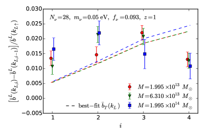
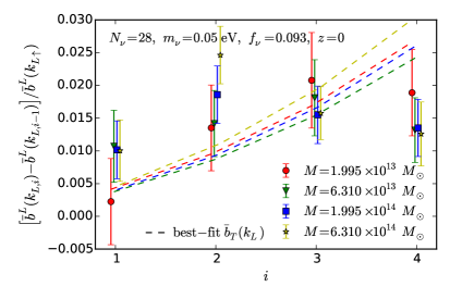
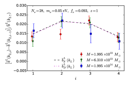
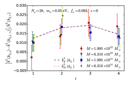
We can further quantify how well the models fit the measurement including the covariance between points by computing

$$\chi^{2} = \sum_{ij}\left[C^{-1}\right]_{ij}\left[D(k_{L,i})-M(k_{L,i})\right]$$ (36)

$$\times\left[D(k_{L,i})-M(k_{L,i})\right]\,,$$

where $i,j$ run over the five values of $k_{L}$, $D(k_{L,i})=\langle\hat{\bar{b}}^{L}(k_{L,i})/\hat{\bar{b}}^{L}(k_{L\uparrow})\rangle$ is the mean of the measured Lagrangian response bias step, $C^{-1}$ is the inverse covariance matrix of $D$, and $M$ is the model of $\bar{b}_{S}^{L}$, $\bar{b}_{D}^{L}$, and $\bar{b}_{T}$. Since we adopt the same Gaussian random realizations for setting up the initial conditions of SU simulations with different $k_{L}$, $D$ of different $k_{L}$ are highly correlated and so it is necessary to use the full covariance matrix to unbiasedly compute $\chi^{2}$. We estimate the covariance matrix by bootstrap resampling the identical realizations for all five $k_{L}$ and repeating the procedure 8,000 times. By definition the first data point of the Lagrangian response bias step has zero variance and no contribution to $\chi^{2}$ (see Fig. 7), so we only consider the rest of the four $k_{L}$. For $\bar{b}_{T}(k_{L})$, there is one fitting parameter so the degrees of freedom (d.o.f.) is three; $\bar{b}_{S}^{L}(k_{L})$ and $\bar{b}_{D}^{L}(k_{L})$ do not contain fitting parameters so d.o.f. is four.

$~{}z~{}$	$~{}M\ [M_{\odot}]~{}$	$~{}\bar{b}_{S}^{L}(k)~{}$	$~{}\bar{b}_{D}^{L}(k)~{}$	$~{}\bar{b}_{T}(k)~{}$
1	$2.0\times 10^{13}$	2.17	1.89	9.92
	$6.3\times 10^{13}$	0.74	0.61	12.6
	$2.0\times 10^{14}$	0.86	0.81	14.7
0	$2.0\times 10^{13}$	1.37	1.28	0.77
	$6.3\times 10^{13}$	0.78	0.65	2.64
	$2.0\times 10^{14}$	0.85	0.75	7.19
	$6.3\times 10^{14}$	0.64	0.66	9.80

Table 2: Summary of the reduced $\chi^{2}$ ($\chi^{2}$/d.o.f.) for the three bias models. Both $\bar{b}_{S}^{L}(k)$ and $\bar{b}_{D}^{L}(k)$ have d.o.f.=4, whereas $\bar{b}_{T}(k)$ has d.o.f.=3.

Tab. 2 summarizes the reduced $\chi^{2}$ ($\chi^{2}$/d.o.f.) for the three bias models. We find that even with one additional fitting parameter, $\bar{b}_{T}(k_{L})$ is generally a very poor fit, especially for halos with high bias, i.e. at high redshift and with high mass. It only works well for halos with the lowest mass at $z=0$. We can therefore rule out transfer function bias as a model for the scale-dependent bias of the SU simulations with high confidence. On the other hand, $\bar{b}_{S}^{L}(k_{L})$ and $\bar{b}_{D}^{L}(k_{L})$ give reasonable values of reduced $\chi^{2}$ except for halos with mass $2\times 10^{13}~{}M_{\odot}$ at $z=1$. Note that the bootstrap construction of the covariance is a noisy estimate so even this case is not necessarily significant. In Fig. 8, we also show that $\bar{b}_{S}^{L}$ and $\bar{b}_{D}^{L}$ predict fairly well the linear trend of the step amplitude with $N_{\nu}$.

The transfer function model fails because it has a transition centered at higher $k_{L}$ than the data requires. The transfer function ratio represents the ratio of CDM and neutrino linear density fluctuations at the observed redshift. Since the free-streaming scale, above which the two are the same, decreases with time this model underestimates the effect of scale-dependent growth at earlier times. On the other hand, both the spherical collapse and universal mass function models automatically incorporate the whole past growth history of the long-wavelength mode. This distinction is even more dramatic at $a\gg 1$ when the transfer functions coincide across the whole linear regime so that $\bar{b}_{T}$ predicts no scale-dependent bias. In the spherical collapse and universal mass function models, once the scale dependence is imprinted in the Lagrangian bias, it remains although in the Eulerian bias it can only be measured for sufficiently rare, high-mass halos where the Lagrangian bias is large compared to unity.

More generally, the failure of the transfer function model indicates that halo bias is temporally nonlocal Hui and Parfrey (2008); Parfrey et al. (2011); LoVerde (2014a, b); Senatore (2015). It is not sufficient to know the properties of the long-wavelength perturbation at just the observation epoch. To make a precise prediction of the scale-dependent bias, one needs to know the whole growth history of $\delta_{c}(a)$.

VI Effects on observables

Because of the scale-dependent responses, the small-scale observables are affected correspondingly. In this section we study how the linear halo power spectrum and squeezed-limit bispectrum are influenced.

Let us start with the linear halo power spectrum. In Sec. V, we have shown that the Lagrangian bias follows to good approximation the growth response $d\ln D_{W}/d\delta_{c}$ as a function of $k_{L}$ which in turn takes the form of a step across the neutrino free-streaming scale of amplitude

$$\frac{\bar{b}^{L}(k_{L\downarrow})}{\bar{b}^{L}(k_{L\uparrow})}=1+Af_{\nu}+B\,,$$ (37)

with $A\approx 0.6$ and $B\approx 0.003$ calculated from $d\ln D_{W}/d\delta_{c}$ at $z=0$. This allows us to extrapolate the simulation results which have an unrealistic $N_{\nu}=14$ and 28 to more relevant lower values. In this section we choose $m_{\nu}=0.05~{}{\rm eV}$, $N_{\nu}=3$, $\Omega_{b}=0.05$, and $\Omega_{c}=0.25$, which corresponds to $f_{\nu}=0.011$. Note that the crude empirical fit to the response bias results give slightly different values of $A\approx 0.5$ and $B\approx 0.0075$, predicting a larger effect in the untested but cosmologically relevant region of $N_{\nu}\lesssim 10$. A finite $B$ represents the scale-dependent bias from the photons rather than neutrinos. To be conservative, when displaying results in this section we set $A=0.6$ and $B=0$ to focus on the neutrino induced bias effects, though we leave our expressions general. Also note that the scaling with $f_{\nu}$ in Eq. (37) is at fixed $m_{\nu}$ and varying $N_{\nu}$. This should not be conflated with fixed $N_{\nu}$ and varying $m_{\nu}$, which would change the free-streaming scale.

Figure 11: Step in bias between $k_{L\uparrow}=0.0005~{}{\rm Mpc}^{-1}$ and $k_{L\downarrow}=0.05~{}{\rm Mpc}^{-1}$ as a function of Eulerian bias $\bar{b}$ (evaluated at $k_{L\uparrow}$) for $A=0.6$, $B=0$, and $f_{\nu}=0.011$. The blue dashed and red solid lines show the Lagrangian and Eulerian bias, respectively. The green circle and black star correspond respectively to $\bar{b}=2$ (LRG/CMASS) and 3.5 (quasar).

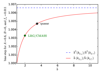
The observed halo bias is in Eulerian space, so we convert the step amplitude in the Lagrangian bias to equivalent in the Eulerian bias

$$\frac{\bar{b}(k_{L\downarrow})}{\bar{b}(k_{L\uparrow})}\> =\frac{\bar{b}^{L}(k_{L\downarrow})+1}{\bar{b}^{L}(k_{L\uparrow})+1}=\left(1-\frac{1}{\bar{b}}\right)\frac{\bar{b}^{L}(k_{L\downarrow})}{\bar{b}^{L}(k_{L\uparrow})}+\frac{1}{\bar{b}}$$

$$=\left(1-\frac{1}{\bar{b}}\right)(1+Af_{\nu}+B)+\frac{1}{\bar{b}}\,,$$ (38)

where $\bar{b}$ is the Eulerian bias evaluated as $k_{L\uparrow}$. Fig. 11 shows the Eulerian (red solid) and Lagrangian (blue dashed) bias step as a function of $\bar{b}$ for $A=0.6$, $B=0$, and $f_{\nu}=0.011$. Unlike the Lagrangian bias step, the Eulerian bias step shows a strong dependence on the value of the bias and hence halo mass. For $\bar{b}=1$, the Lagrangian bias is zero, so the scale dependence vanishes; for $\bar{b}\gg 1$, the Eulerian bias step approaches to the Lagrangian bias step, meaning the impact of the scale-dependent bias on the clustering of halos is most significant in high bias, high mass objects for $\bar{b}\geq 1$. The green circle and black star correspond to objects of $\bar{b}=2$ (LRG/CMASS Marin (2011); Gil-Marín et al. (2015)) and 3.5 (quasar Eftekharzadeh et al. (2015)). While the net effect for $f_{\nu}=0.011$ is quite small, we shall see next that it has a significant effect on the linear halo power spectrum relative to the also small step in the linear CDM power spectrum.

Figure 12: Decrease of linear halo power spectrum suppression due to neutrino scale-dependent bias at $k_{L\downarrow}$, i.e. $R_{hh}$, as a function of $\bar{b}$ for $A=0.6$. The green circle and black star correspond to $\bar{b}=2$ (LRG/CMASS) and 3.5 (quasar).

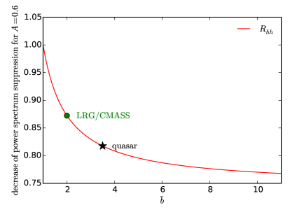
Since our bias is defined with respect to the underlying CDM(+baryon) field instead of total matter (including massive neutrinos), the linear halo power spectrum is given by $P_{hh}=\bar{b}^{2}P_{cc}$, where $P_{cc}(k)$ is the linear CDM power spectrum. Neutrinos suppress the growth of CDM perturbations and produce a downward step in its power spectrum with respect to the $m_{\nu}=0$ model with the same total nonrelativistic matter. The amplitude of the full step is approximately $\Delta P_{cc}/P_{cc}\approx-6f_{\nu}$, but as we have seen in Sec. V the step in the CDM transfer function is not fully complete by $k_{L\downarrow}$ where the step in bias is essentially complete. For an accurate comparison, we use CLASS to compute the linear power spectrum for $N_{\nu}=3$ massless neutrinos with $\Omega_{c}=0.253$, and find

$$\frac{P_{cc}(k_{L\downarrow})}{P_{cc}^{m_{\nu}=0}(k_{L\downarrow})}\approx 1-4.7f_{\nu}\,.$$ (39)

Using Eq. (38) and linearizing in $f_{\nu}$, we find the suppression in linear halo power spectrum becomes

$$\frac{P_{hh}(k_{L\downarrow})}{P_{hh}^{m_{\nu}=0}(k_{L\downarrow})}\approx 1-4.7R_{hh}(\bar{b})f_{\nu}+2\left(1-\frac{1}{\bar{b}}\right)B\,,$$ (40)

where

$$R_{hh}(\bar{b})=1-\frac{2A}{4.7}\left(1-\frac{1}{\bar{b}}\right)\,.$$ (41)

The decrease of the linear halo power spectrum suppression relative to CDM due to neutrino induced scale-dependent bias is captured by $R_{hh}(\bar{b})$. Fig. 12 shows $R_{hh}(\bar{b})$ for $A=0.6$. We find that for LRG/CMASS and quasars the decrease of linear halo power spectrum suppression is 13% and 18%, respectively. In the limit that $\bar{b}\gg 1$, the reduction is 26%. Of course the observed halo and mass power spectra also involve nonlinear corrections with their own scale dependence. Nonetheless the scale-dependent linear bias thus should be taken into account whenever neutrino growth suppression is considered in galaxy survey data for any $f_{\nu}$ if the free-streaming scale is deep in the linear regime as it is for $m_{\nu}=0.05~{}{\rm eV}$.

Let us now turn to the squeezed-limit bispectrum. Unlike the linear halo power spectrum, the halo bispectrum at the leading order contains the contribution from the nonlinear bias, which can be regarded as the response of the linear bias to $\delta_{c}$ (e.g. Ref. Chiang (2017)). Accurate calibration of higher-order responses requires SU simulations with larger $|\delta_{c0}|$ Wagner et al. (2015b); Lazeyras et al. (2016). Lacking such simulations, we thus consider only one piece of the halo bispectrum and set $B_{hhh}^{\rm sq}(k,k_{L})=\bar{b}^{2}(k)\bar{b}(k_{L})B_{ccc}^{\rm sq}(k,k_{L})$ with $B_{ccc}$ being the CDM bispectrum. Furthermore, to highlight the effect from the scale-dependent growth response, we only show the result for the CDM squeezed-limit bispectrum, i.e.

$$B^{\rm sq}_{ccc}(k,k_{L})\> =\langle P_{cc}(k|\tilde{\delta}_{c}(k_{L}))\tilde{\delta}_{c}(k_{L})\rangle$$

$$=R_{\rm tot}(k,k_{L})P_{cc}(k)P_{cc}(k_{L})\,,$$ (42)

where $k$ and $k_{L}$ are the small- and large-scale modes, $P_{cc}(k|\tilde{\delta}_{c}(k_{L}))$ is the CDM power spectrum in the presence of a single long-wavelength mode of Fourier amplitude $\tilde{\delta}_{c}$ and wavenumber $k_{L}$. As pointed out in Sec. IV.1, the total power spectrum response $R_{\rm tot}$ contains the contributions from the growth response $R_{\rm growth}$, that can be measured from the SU simulations, as well as dilation and reference-density effects. To the leading order, $R_{\rm dilation}$ and $R_{\bar{\rho}}$ are given by

$$R_{\rm dilation}(k)=-\frac{1}{3}\frac{d\ln k^{3}P(k)}{d\ln k}\,,\quad R_{\bar{\rho}}=2\,,$$ (43)

which are independent of $k_{L}$. Therefore, the step feature in the squeezed-limit bispectrum due to the scale-dependent growth response is diluted by $R_{\rm dilation}$ and $R_{\bar{\rho}}$.

Figure 13: Step of CDM power spectrum response as a function of the long mode $k_{L}$. The red solid, green dashed, and blue dot-dashed lines show the step of the total power spectrum response, equivalent to the reduced squeezed-limit bispectrum, with the short mode $k=0.2$, 0.3, and 0.4 Mpc, whereas the black dotted line shows the growth response alone.

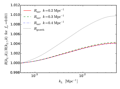
In Sec. IV.2 we have shown that the growth responses measured from the SU simulations of $N_{\nu}=14$ and 28 are in excellent agreement with the analytic calculation. Thus, for $f_{\nu}=0.011$ cosmology we assume $R_{\rm growth}=2(d\ln D_{W}/d\delta_{c})$, which depends only on $k_{L}$. For $R_{\rm dilation}$, we use the spectral index of the CDM power spectrum, which depends on $k$. Fig. 13 shows the power spectrum response as a function of the long mode $k_{L}$. The red solid, green dashed, and blue dot-dashed lines show the step of the total power spectrum response, equivalent to the reduced squeezed-limit bispectrum, with the short mode $k=0.2$, 0.3, and $0.4~{}{\rm Mpc}^{-1}$, whereas the black dotted line shows the growth response alone. As expected, $R_{\rm dilation}$ and $R_{\bar{\rho}}$ dilute the dependence on $k_{L}$, and compared to $R_{\rm growth}$ the step size is reduced by 60%. Albeit small, the scale dependence is a distinct feature due to massive neutrinos, hence can serve as an independent probe. On the other hand, we find that $R_{\rm tot}$ depends only weakly on $k$. This is because for $k\gtrsim 0.2~{}{\rm Mpc}^{-1}$ the baryonic acoustic oscillation is less prominent, and so the spectral index is closer to a constant.

Our discussion focuses on the galaxy squeezed-limit bispectrum, but the derivation is similar for the galaxy-galaxy-lensing bispectrum (see Ref. Chiang and Slosar (2017) for the cross-correlation between Lyman-$\alpha$ power spectrum and lensing convergence), where the lensing convergence provides the long mode. Since lensing measures the total matter fluctuation along the line-of-sight, the bispectrum is schematically given by $B^{\rm sq}_{hhm}(k,k_{L})=\bar{b}^{2}(k)B^{\rm sq}_{ccm}(k,k_{L})$, where the CDM-CDM-matter squeezed-limit bispectrum is given by

$$B^{\rm sq}_{ccm}(k,k_{L})\> \equiv\langle P_{cc}(k|\tilde{\delta}_{m}(k_{L}))\tilde{\delta}_{m}(k_{L})\rangle$$

$$=R_{\rm tot}(k,k_{L})P_{cc}(k)P_{cm}(k_{L})\,.$$ (44)

Here we have assumed that since the perturbations are adiabatic, there is a one-to-one relation between the long-wavelength $\tilde{\delta}_{m}$ and $\tilde{\delta}_{c}$ given by the linear transfer functions so that

$$\frac{d\ln P_{cc}(k)}{d\delta_{m}}(k_{L})\> =R_{\rm tot}(k,k_{L})\frac{T_{c}(k_{L})}{T_{m}(k_{L})}\,,$$

$$P_{cm}(k_{L})\> =\frac{T_{c}(k_{L})}{T_{m}(k_{L})}P_{mm}(k_{L})\,.$$ (45)

We find that the only difference between the $B^{\rm sq}_{ccc}$ and $B^{\rm sq}_{ccm}$ is the large-scale power spectra, i.e. $P_{cc}(k_{L})$ versus $P_{cm}(k_{L})$.

VII Discussion

Massive neutrinos provide an ideal arena to explore the scale dependence of the response of small-scale structure formation to the large-scale density environment. Due to their large thermal velocities, massive neutrino fluctuations track the CDM only on scales larger than the free-streaming scale with smaller-scale fluctuations washed out. As a result, the growth of CDM perturbations becomes scale dependent. The response of small-scale observables to these long-wavelength perturbations consequently becomes scale dependent as well. These effects can be captured in the separate universe (SU) technique by absorbing the long-wavelength perturbations into the local expansion.

Using the SU technique, we perform $N$-body simulations in overdense and underdense SUs with different wavelengths of the large-scale CDM density perturbations in a universe with massive neutrinos. By differencing pairs of overdense and underdense SU simulations with the same Gaussian realizations of initial phases, we measure how the power spectrum and halo mass function respond to large-scale CDM density perturbations of different wavelengths, which give rise to the squeezed-limit bispectrum and the halo bias, respectively. Due to the cancellation of the cosmic variance, the SU simulations yield a precise characterization of the scale dependence of these responses.

Specifically, for the cosmology with $m_{\nu}=0.05~{}{\rm eV}$ but an artificially high number of neutrinos totaling a fraction $f_{\nu}=0.093$ of the matter, we perform SU simulations for five long-wavelength perturbations (from $k_{L\uparrow}=0.0005~{}{\rm Mpc}^{-1}$ to $k_{L\downarrow}=0.05~{}{\rm Mpc}^{-1}$) spanning the free-streaming transition. Scale dependence in the responses for the power spectrum and Lagrangian bias are detected with high significance (see Fig. 4 and Fig. 7). Interestingly, we find that the scale dependence in both cases can be described well with just the linear growth response, which can be calculated without simulations and with no free parameters. For Lagrangian bias, this result follows if the mass function is universal in the local power spectrum but is also equally consistent with the spherical collapse model. To further confirm this result, we also perform SU simulations with $f_{\nu}=0.049$ for $k_{L\uparrow}$ and $k_{L\downarrow}$ (see Fig. 5 and Fig. 8) and show that they are consistent with the linear growth response as well, implying a scaling of the steps across the free streaming scale of $\sim 0.6f_{\nu}$. This scaling allows us to extrapolate our results to a more realistic case of three massive neutrinos of $0.05~{}{\rm eV}$ with $f_{\nu}=0.011$.

There are two important implications of our results. First, the scale-dependent responses due to massive neutrinos produce new features in the halo power spectrum and squeezed-limit bispectrum, and the effects are shown in Figs. 12-13 with $f_{\nu}=0.011$. For the linear halo power spectrum, we find that the scale-dependent bias reduces the difference between linear power spectra of massive and massless neutrinos by 13 and 26% for objects of $\bar{b}=2$ and $\bar{b}\gg 1$, respectively independently of $f_{\nu}$. The larger the halo mass (hence the halo bias), the larger effect due to the scale-dependent bias. This effect must be taken into account for future surveys that use the halo power spectrum to constrain neutrino mass LoVerde (2016). For the CDM-CDM-CDM reduced squeezed-limit bispectrum, we find that the step size is around 4% with a weak dependence on the small-scale mode $k$. The effect is small because the dilation and reference-density responses dilute the scale dependence from the growth response. Albeit small, the scale dependence is a distinct characteristic due to massive neutrinos can be used as an independent probe.

Second, we find that halo bias is temporally nonlocal. For the same value of the CDM density fluctuations at two different wavenumbers, the bias differs due to the evolutionary histories of the modes. A local model of density bias, even one that allows for local bias with respect to the different density components cannot describe this effect. Specifically, we demonstrate in Figs. 9-10 that the transfer function bias $\bar{b}_{T}(k)=b_{c}+b_{\nu}\left[T_{\nu}(k)/T_{c}(k)\right]$, where $b_{c}$ and $b_{\nu}$ are the CDM and neutrino bias parameters and $T_{c}$ and $T_{\nu}$ are the CDM+baryon and neutrinos transfer functions, is a poor fit to the scale-dependent bias measured from our SU simulations for any $b_{c}$ and $b_{\nu}$. Therefore, the standard Lagrangian picture that the halo statistics at any time are determined entirely by the linear density field at a single epoch is falsified in this case where the free-streaming or Jeans scale is deeply in the linear regime.

Our SU simulations assume a fixed and low value of the individual neutrino masses $m_{\nu}=0.05~{}{\rm eV}$ and should not be naively extrapolated to higher values. Since the SU ignores small-scale neutrino clustering, the free-streaming scale must be much larger than the scale of the observables. For $m_{\nu}=0.05~{}{\rm eV}$ we argue in App. C that neutrino clustering can be neglected for $k\gtrsim 0.05~{}{\rm Mpc}^{-1}$. Furthermore, since we approximate the long-wavelength mode as spatially constant, it must also be much larger than the region that encompasses the small-scale observables. Specifically for halo bias, corrections will enter at $\mathcal{O}(k_{L}^{2}R_{M}^{2})$ with $R_{M}$ being the Lagrangian radius of halo with mass $M$ and for the power spectrum response $\mathcal{O}(k_{L}^{2}/k^{2})$ with $k_{L}$ and $k$ being the wavenumbers of the large- and small-scale modes respectively.

With too small a free-streaming scale, these limitations would make it impossible to track responses across the free-streaming scale with the SU technique. Even for $m_{\nu}=0.05~{}{\rm eV}$, we expect there to be some correction to our results from the clustering of slow neutrinos in the tail of the neutrino distribution function (see discussion in Ref. Senatore and Zaldarriaga (2017)) and the scale dependence of power spectra from nonlinearity. In App. E we compare our prediction to one of the best suites of $N$-body simulations with massive neutrino particles, and find that it is equally consistent with the neutrino particle simulations as the scale-independent linear bias. As discussed in more detail there, to distinguish our novel scale dependence it is necessary to run neutrino particle simulations of a few Gpc, to see the full scale dependence at large scales, and with high enough $f_{\nu}$ or a large enough number of simulations to robustly constrain the $\mathcal{O}(f_{\nu})$ corrections discussed here. Note that $f_{\nu}$ should be increased while keeping $m_{\nu}\sim 0.05$ eV so that the free-streaming scale and nonlinear clustering of neutrinos are not qualitatively changed. We leave the detailed comparison between our SU results with other techniques of simulating massive neutrinos for future work.

Appendix A Robustness to initial conditions

In this appendix we test the choice of initial and horizon-entry scale factors, $a_{i}$ and $a_{H}$, for solving the differential equation of the small-scale growth, i.e. Eqs. (8)–(9). We shall particularly focus on the growth response at $a\geq 0.02$, as it corresponds to the quantity observable and time of interest.

Figure 14: Fractional difference of the growth response of various $a_{H}$ to that with $a_{H}=10^{-10}$, for fixed $a_{i}=10^{-6}$ and two limiting $k_{L}$.

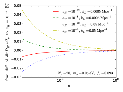
Following the discussion in Sec. II.2, we have the constraint $a_{\rm eq}\gg a_{i}\gg a_{H}$. Let us start by fixing $a_{i}=10^{-6}$ and varying $a_{H}=10^{-12}$, $10^{-10}$, and $10^{-8}$. Fig. 14 shows the fractional difference of the growth response of various $a_{H}$ to that with $a_{H}=10^{-10}$, for fixed $a_{i}=10^{-6}$ and two limiting $k_{L}$. We find that for all cases the differences are less than 0.05%, and the agreement is better for $a$ approaching to unity. This demonstrates that the difference due to $a_{H}$ can be safely neglected and justifies our choice of $a_{H}=10^{-10}$ in the main text.

Figure 15: Same as Fig. 14, but for various $a_{i}$ to that with $a_{i}=10^{-6}$, for fixed $a_{H}=10^{-10}$.

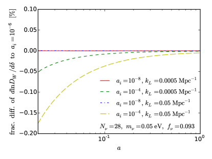
We next fix $a_{H}=10^{-10}$, and compute the growth response with $a_{i}=10^{-4}$, $10^{-6}$, and $10^{-8}$. Note that unlike the $a_{H}$ dependence, which corresponds to a true dependence on the short-wavelength $k$ that cannot be captured in our SU implementation, this tests a purely computational error from assuming $a_{i}\ll a_{\rm eq}$ in the derivation. Fig. 15 shows the fractional difference of the growth response of various $a_{i}$ to that with $a_{i}=10^{-6}$, for fixed $a_{H}=10^{-10}$ and two limiting $k_{L}$. We first find that the agreement is good between $a_{i}=10^{-6}$ and $10^{-8}$, indicating the convergence for even earlier $a_{i}$. Between $a_{i}=10^{-6}$ and $10^{-4}$, the differences at $a=0.02$ (initial redshift of the SU simulations) are apparent. This justifies our choice of $a_{i}=10^{-6}$ used in the main text.

Appendix B 2LPT in the separate universe

In this appendix, we derive the small-scale growth of the displacement field under the framework of 2LPT, assuming that CDM is the only component that clusters (e.g. below the Jeans scales of all other clustering components), in order to set up the initial conditions of the SU simulations. Following the standard convention in App. D of Ref. Scoccimarro (1998), we define $D_{1}$ and $D_{2}$ to be the growths of the first and second order perturbations of the displacement field. In the absence of the long-wavelength perturbation $\delta_{c}$, the evolution of $D_{1}$ and $D_{2}$ are given by

$$D^{\prime\prime}_{1}+\left(2+\frac{H^{\prime}}{H}\right)D^{\prime}_{1}-\frac{3}{2}\Omega_{c}(a)D_{1}=0\,,$$ (46)

$$D^{\prime\prime}_{2}+\left(2+\frac{H^{\prime}}{H}\right)D^{\prime}_{2}-\frac{3}{2}\Omega_{c}(a)D_{2}=-\frac{3}{2}\Omega_{c}(a)D_{1}^{2}\,.$$ (47)

Note that the equation of the first order growth is identical to Eq. (8). If we set the initial conditions of the differential equations at $a_{i}$ during the matter-dominated epoch, then $H^{\prime}/H=-3/2$ and if CDM dominates the matter density then $\Omega_{c}(a)=1$; hence we obtain the standard results (e.g. Bouchet et al. (1995); Scoccimarro (1998); Crocce et al. (2006)):

$$D_{1}(a_{i})=a_{i}\,,\quad D^{\prime}_{1}(a_{i})=a_{i}\,,$$

$$D_{2}(a_{i})=-\frac{3}{7}a_{i}^{2}\,,\quad D^{\prime}_{2}(a_{i})=-\frac{6}{7}a_{i}^{2}\,.$$ (48)

On the other hand, if $a_{i}$ is in the radiation-dominated epoch, then $(2+H^{\prime}/H)\propto a_{i}/a_{\rm eq}\to 0$ and $\Omega_{c}(a)\propto a_{i}/a_{\rm eq}\to 0$, and the solutions to the small-scale growths become

$$D_{1}(a_{i})=\ln\frac{a_{i}}{a_{H}}\,,\quad D^{\prime}_{1}(a_{i})=1\,,$$

$$D_{2}(a_{i})=-\frac{3}{2}\Omega_{c}(a)\left[\left(\ln\frac{a_{i}}{a_{H}}\right)^{2}-4\ln\frac{a_{i}}{a_{H}}+6\right]\,,$$

$$D^{\prime}_{2}(a_{i})=-\frac{3}{2}\Omega_{c}(a)\left[\left(\ln\frac{a_{i}}{a_{H}}\right)^{2}-2\ln\frac{a_{i}}{a_{H}}+2\right]\,.$$ (49)

Let us now turn to the universe with a long-wavelength perturbation $\delta_{c}$. Within the SUs the small-scale growths of 2LPT follow

$$\frac{d^{2}D_{W1}}{d\ln a_{W}^{2}}+\left(2+\frac{d\ln H_{W}}{d\ln a_{W}}\right)\frac{dD_{W1}}{d\ln a_{W}}$$

$$\hskip 14.22636pt-\frac{3}{2}\frac{H_{0W}^{2}}{H_{W}^{2}}\frac{\Omega_{cW}}{a_{W}^{3}}D_{W1}=0\,,$$ (50)

$$\frac{d^{2}D_{W2}}{d\ln a_{W}^{2}}+\left(2+\frac{d\ln H_{W}}{d\ln a_{W}}\right)\frac{dD_{W2}}{d\ln a_{W}}$$

$$\hskip 14.22636pt-\frac{3}{2}\frac{H_{0W}^{2}}{H_{W}^{2}}\frac{\Omega_{cW}}{a_{W}^{3}}D_{W2}=-\frac{3}{2}\frac{H_{0W}^{2}}{H_{W}^{2}}\frac{\Omega_{cW}}{a_{W}^{3}}D_{W1}^{2}\,.$$ (51)

Rewriting the differential equations in terms of the global coordinate and linearizing in $\delta_{c}$, we have the perturbations to the growths $\epsilon_{1}=D_{W1}-D_{1}$ and $\epsilon_{2}=D_{W2}-D_{2}$ to be

$$\epsilon^{\prime\prime}_{1}+\left(2+\frac{H^{\prime}}{H}\right)\epsilon^{\prime}_{1}-\frac{3}{2}\Omega_{c}(a)\epsilon_{1}$$

$$\hskip 14.22636pt=\frac{2}{3}\delta_{c}^{\prime}D^{\prime}_{1}+\frac{3}{2}\Omega_{c}(a)\delta_{c}D_{1}\,,$$ (52)

$$\epsilon^{\prime\prime}_{2}+\left(2+\frac{H^{\prime}}{H}\right)\epsilon^{\prime}_{2}-\frac{3}{2}\Omega_{c}(a)\epsilon_{2}$$

$$\hskip 14.22636pt=\frac{2}{3}\delta_{c}^{\prime}D^{\prime}_{2}+\frac{3}{2}\Omega_{c}(a)\left[\delta_{c}(D_{2}-D_{1}^{2})-2D_{1}\epsilon_{1}\right]\,.$$ (53)

To solve $\epsilon_{1}$ and $\epsilon_{2}$ in the matter-dominated universe, we assume that $\delta_{c}$ is sub-horizon and so proportional to $a$, which leads to

$$\epsilon_{1}(a_{i})=\frac{13}{21}\delta_{c}(a_{i})D_{1}(a_{i})\,,\quad\epsilon^{\prime}_{1}(a_{i})=\frac{26}{21}\delta_{c}(a_{i})D_{1}(a_{i})\,,$$

$$\epsilon_{2}(a_{i})=\frac{32}{27}\delta_{c}(a_{i})D_{2}(a_{i})\,,\quad\epsilon^{\prime}_{2}(a_{i})=\frac{32}{9}\delta_{c}(a_{i})D_{2}(a_{i})\,.$$ (54)

On the other hand, for the radiation-dominated universe we assume that $\delta_{c}$ is super-horizon and so proportional to $a^{2}$. This then leads to

$$\epsilon_{1}(a_{i})=\frac{1}{3}\delta_{c}(a_{i})D^{\prime}_{1}(a_{i})\,,\quad\epsilon^{\prime}_{1}(a_{i})=\frac{2}{3}\delta_{c}(a_{i})D^{\prime}_{1}(a_{i})\,,$$

$$\epsilon_{2}(a_{i})=-\frac{3}{2}\Omega_{c}(a_{i})\delta_{c}(a_{i})\left[D^{\prime}_{1}(a_{i})\right]^{2}$$

$$\hskip 36.98866pt\left[\frac{7}{27}\ln\left(\frac{a_{i}}{a_{H}}\right)^{2}-\frac{46}{81}\ln\frac{a_{i}}{a_{H}}+\frac{50}{81}\right]\,,$$

$$\epsilon^{\prime}_{2}(a_{i})=-\frac{3}{2}\Omega_{c}(a_{i})\delta_{c}(a_{i})\left[D^{\prime}_{1}(a_{i})\right]^{2}$$

$$\hskip 36.98866pt\left[\frac{7}{9}\ln\left(\frac{a_{i}}{a_{H}}\right)^{2}-\frac{32}{27}\ln\frac{a_{i}}{a_{H}}+\frac{104}{81}\right]\,.$$ (55)

Note that the results of $D_{1}(a_{i})$ and $\epsilon_{1}(a_{i})$ are identical to Eq. (13).

For our SU simulations, we first set the initial conditions of the small-scale growths at $a_{i}=10^{-6}$, with $a_{H}=10^{-10}$. We then evolve the differential equations to the initial redshift of the simulations at $a_{Wi}(\delta_{c0})=0.02$. Since usually the code for setting up the initial conditions of $N$-body simulations uses growth rate for the velocities of particles, we rewrite

$$f_{W1}\> =\frac{d\ln D_{W1}}{d\ln a_{W}}=\left(1+\frac{1}{3}\delta^{\prime}_{c}\right)\frac{D^{\prime}_{1}+\epsilon^{\prime}_{1}}{D_{1}+\epsilon_{1}}\,,$$

$$f_{W2}\> =\frac{d\ln D_{W2}}{d\ln a_{W}}=\left(1+\frac{1}{3}\delta^{\prime}_{c}\right)\frac{D^{\prime}_{2}+\epsilon^{\prime}_{2}}{D_{2}+\epsilon_{2}}\,.$$ (56)

Appendix C Separate universe systematics

C.1 Neutrino clustering

Figure 16: Ratio of the typical amplitude of (linear) neutrino perturbations to total matter perturbations. This quantifies the error (in units of $f_{\nu}$) induced on the density field on scale $k$ from assuming that neutrinos are completely smooth in our simulations. This plot uses $N_{\nu}=28$ neutrinos $(f_{\nu}=0.093)$ but we find that the results are only weakly dependent on the number of neutrinos.

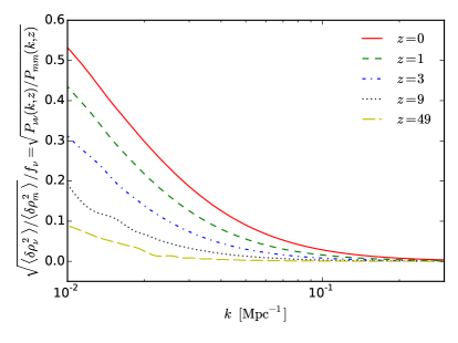
The separate universe approach used in this paper assumes that the neutrino energy density is completely smooth within the simulations box. For our choice of box size $L=700$ Mpc, neutrinos are clustered at late times on the largest scales so our simulations are missing some neutrino perturbations on the largest scales. These scales are in the linear regime so we can straightforwardly estimate the scale at which neutrino perturbations are important from their fractional contribution to the total gravitational potential as a function of $k$ using the linear power spectrum

$$\frac{\Delta\Phi_{\nu}(k)}{\Phi}\approx\sqrt{\frac{\langle\delta\rho_{\nu}(k)^{2}\rangle}{\langle\delta\rho_{m}(k)^{2}\rangle}}=f_{\nu}\sqrt{\frac{P_{\nu\nu}(k)}{P_{mm}(k)}}\,.$$ (57)

This quantity is plotted in Fig. 16. We can see that so long as we restrict our attention to $k\gtrsim 0.05~{}{\rm Mpc}^{-1}$ the error due to neglecting neutrino clustering should be $\lesssim 0.1f_{\nu}$. Note that the “missing” neutrino perturbations are absent in each of the SU simulations ($\delta_{c0}=\pm 0.01,0$ for each $k_{L}$) so the absolute error on the response quantities determined from differences between simulations should be even smaller. In this paper we only report the power spectrum response with $k\geq 0.05~{}{\rm Mpc}^{-1}$.

Figure 17: The velocity distribution of a single species of neutrinos with mass $0.05~{}{\rm eV}$ at several redshifts. Vertical dashed lines show the escape velocities of dark matter halos of several masses.

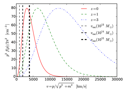
We have seen that the error from neglecting the large-scale linear theory neutrino perturbations should be small ($\mathcal{O}(0.1f_{\nu})$). On smaller scales where the CDM perturbations have become nonlinear, however, one could worry that the gravitational potentials are strong enough to cause significant clustering of slow-moving neutrinos.

In Fig. 17, we show the mean velocity distribution of neutrinos at several epochs in comparison with the escape velocities of dark matter halos. We define the escape velocities as $v_{\rm sec}\equiv\sqrt{2[\Phi(r=\infty)-\Phi(r=R_{s})]}$ where $\Phi$ is the gravitational potential of a Navarro, Frenk, and White dark matter halo Navarro et al. (1997) and $R_{s}$ is the scale radius of the halo. At the latest times, a significant fraction of neutrinos can indeed become bound, or at least significantly deflected, by nonlinear structure. On the other hand, the relative contribution of these neutrinos to the total gravitational potential remains small since the CDM perturbations on the same scale are large. For instance, for halos with virial masses $M=10^{13}$, $10^{14}$, and $10^{15}M_{\odot}$, the local overdensity of neutrino mass for each mass state is approximately $10^{8}$, $3\times 10^{9}$, and $10^{11}~{}M_{\odot}$ respectively LoVerde and Zaldarriaga (2014). Hence, even for our simulations with $N_{\nu}=28$, the fractional correction to the gravitational potential, and therefore the evolution the CDM particles is $\sim 0.003f_{\nu}$, $0.01f_{\nu}$, and $0.03f_{\nu}$ for the halo masses $M=10^{13}$, $10^{14}$, and $10^{15}M_{\odot}$. This estimate is consistent with Ref. LoVerde (2014b), which found that the effects of neutrino clustering around CDM halos was negligible in spherical collapse calculations so long as the individual neutrino mass $m_{\nu}\lesssim 0.2~{}{\rm eV}$. We thus consider it a safe assumption to ignore the effect of neutrino clustering on halo response bias.

C.2 Large-scale averaging

In the SU approximation we take the wavelength of the large-scale density perturbation to be sufficiently larger than the scale of interest for small-scale observables that its spatially varying amplitude can be replaced by its locally averaged value. In other words we conflate $\delta_{c}$ with $\delta_{cW}$ where

$$\delta_{cW}({\bf x}_{0})=\int d^{3}xW_{R}({\bf x}_{0}-{\bf x})\delta_{c}({\bf x})\,,$$ (58)

and $W_{R}$ is some spherically symmetric window with support on $|{\bf x}_{0}-{\bf x}|\lesssim R$ which is normalized to integrate to unity. In Fourier space

$$\tilde{\delta}_{cW}({\bf k})=\tilde{W}_{R}({\bf k})\tilde{\delta}_{c}({\bf k})\,,$$ (59)

and for wavelengths that are long compared to $R$

$$\lim_{kR\rightarrow 0}\tilde{\delta}_{cW}({\bf k})=\left[1+{\cal O}(k^{2}R^{2})\right]\tilde{\delta}_{c}({\bf k})\,.$$ (60)

At a fixed $k=k_{L}$, the SU approximation is limited to observables that are sensitive to only a region $R\ll 1/k_{L}$. For the halo mass function a rough indication of the region of influence is the Lagrangian radius of the halo $R_{M}$. For the power spectrum the typical scale is $R\sim 1/k$. We thus conclude that averaging errors on the response bias scale as $\mathcal{O}(k_{L}^{2}R_{M}^{2})$, and those on the squeezed bispectrum as $\mathcal{O}(k_{L}^{2}/k^{2})$. Note that these scalings apply to both neutrino and $\Lambda$CDM separate universe simulations but for the former we take $k_{L}\gtrsim k_{\rm fs}$ in order to measure the scale dependence of the responses.

Appendix D Spherical collapse bias

We follow the method of Ref. LoVerde (2014a) to make spherical collapse calculations of the Lagrangian response bias. A region of size $R$ containing a constant mass $M$ of CDM will evolve according to

$$\ddot{R}=\> -\frac{GM(<R)}{R^{2}}$$ (61)

$$-\frac{4\pi G}{3}\sum_{x}\left[\rho_{x}(t)+\delta\rho_{x}+3P_{x}(t)+3\delta P_{x}\right]R\,,$$

where $\dot{\,}\equiv d/dt$, $\rho_{x}$ and $P_{x}$ are the energy density and pressure of any non-CDM components of the universe and $\delta\rho_{x}$, and $\delta P_{x}$ are long-wavelength perturbations in the energy density and pressure of $x$. Using $M=\frac{4}{3}\pi R^{3}\rho_{c}(1+\delta)$, and factoring out a long-wavelength CDM perturbation from $\delta$ allows this equation to be rewritten in terms of the fluctuation from the local mean $\delta_{S}$, defined via $(1+\delta)=[1+\delta_{c}(a)](1+\delta_{S})$ as

$$\frac{d^{2}\delta_{S}}{d\ln a_{W}^{2}}+\left(2+\frac{d\ln H_{W}}{d\ln a_{W}}\right)\frac{d\delta_{S}}{d\ln a_{W}}-\frac{4}{3}\frac{\left(\frac{d\delta_{S}}{d\ln a_{W}}\right)^{2}}{1+\delta_{S}}$$

$$\hskip 14.22636pt\qquad=\frac{3}{2}\frac{\Omega_{cW}H_{0W}^{2}}{a_{W}^{3}H_{W}^{2}}\delta_{S}(1+\delta_{S})\,,$$ (62)

where $a_{W}=a[1-\delta_{c}(a)/3]$, as before. This equation is equivalent to Eq. (61) and can be viewed as a nonlinear generalization of Eq. (7) (for spherical density perturbations). Eq. (62) is identical to the usual nonlinear equation for a spherical density perturbation and the solutions are independent of $M$. For given initial conditions $\delta_{Si}=\delta_{S}(a_{Wi})$ and $\left[d\ln\delta_{S}/d\ln a_{W}\right](a_{Wi})$, it can be solved to determine $a_{{\rm coll},W}$, the SU scale factor at which $\delta_{S}\rightarrow\infty$.

Following our calculations for $D_{W}$ and App. A, we start at $a_{i}=10^{-6}$ with initial velocity

$$\frac{d\ln\delta_{S}}{d\ln a_{W}}(a_{i})=\frac{d\ln D_{W}}{d\ln a_{W}}(a_{i})\,.$$ (63)

We iteratively solve Eq. (62) to determine the initial density perturbation $\delta_{Si}$ that will “collapse” at global scale factor $a_{\rm coll}$ for each $\delta_{c}(a,k_{L})$. Our criteria for collapse is that $d\ln\delta_{S}/d\ln a_{W}=100$. The linearly extrapolated threshold for collapse is given by $\delta_{\rm crit}\equiv\left[D(a_{\rm coll})/D(a_{i})\right]\delta_{Si}$, where the initial value of $\delta_{Si}$ that produces collapse at $a_{\rm coll}$ is a function of the long-wavelength mode $\delta_{c}(a)$. From this we compute

$$\frac{\delta\delta_{\rm crit}}{\delta\delta_{c}}(a_{\rm coll})=\frac{\delta_{\rm crit}(\delta_{c})-\delta_{\rm crit}(-\delta_{c})}{2\delta_{c}(a_{\rm coll})}\,,$$ (64)

and define the Lagrangian bias with respect to CDM as

$$\bar{b}_{S}^{L}=\frac{\partial\ln n(M)}{\partial\delta_{\rm crit}}\frac{\delta\delta_{\rm crit}}{\delta\delta_{c}}(k_{L})\,.$$ (65)

Appendix E Comparison of scale-dependent bias with neutrino particle simulations

In this appendix we compare the scale-dependent bias model based on the response of the halo mass function in SU simulations to the clustering bias measured from $N$-body simulations with massive neutrino particles in Ref. Villaescusa-Navarro et al. (2017). This simulation suite is one of the largest to date and contains 100 realizations of $1~{}h^{-1}~{}{\rm Gpc}$ boxes. The cosmological parameters are $h=0.6711$, $\Omega_{b}=0.049$, and $\Omega_{c}=0.2649$, with three massive neutrinos of 0.05 eV, corresponding to $f_{\nu}=0.011$. The halos are identified with the Friends-of-Friends algorithm Davis et al. (1985), and to be conservative we only consider halos with more than 100 dark matter particles, corresponding to a minimum halo mass of $9.673\times 10^{13}~{}M_{\odot}$. The clustering bias is measured with respect to CDM, i.e. $\bar{q}(k)=P_{ch}(k)/P_{cc}(k)$. We use a Fourier bin of $0.002~{}h~{}{\rm Mpc}^{-1}$ so that the data point are dense enough while we still have enough realizations to estimate the covariance matrix.

We fit the mean of the measured clustering bias to two linear bias models. The first one is that the linear bias is scale independent, hence the total bias is given by

$$\bar{b}(k)=\bar{b}_{1}+\bar{b}_{k^{2}}k^{2}\,,$$ (66)

where the $k^{2}$ term absorbs the loop corrections in the large-scale limit Assassi et al. (2014). We also explore the inclusion of additional $\bar{b}_{k^{4}}k^{4}$ but find no significant difference, so we present the simpler model. The second one is our predicted scale dependence, and the model is given by

$$\bar{b}(k)=1+\bar{b}^{L}_{1}f(k)+\bar{b}_{k^{2}}k^{2}\,,$$ (67)

where we set $f(k)=[d\ln D_{W}/d\delta_{c}](k)/[d\ln D_{W}/d\delta_{c}](k_{\uparrow})$. To compute $f(k)$ we use the same cosmology as in Ref. Villaescusa-Navarro et al. (2017). Note that this model is identical to $\bar{b}^{L}_{D}$ defined in Eq. (31) with an additional $\bar{b}_{k^{2}}$ accounting for the nonlinear correction. Both models contain two free parameters, and we find the parameters by minimizing

$$\chi^{2}=\sum_{ij}[\bar{q}(k_{i})-\bar{b}(k_{i})][\bar{q}(k_{j})-\bar{b}(k_{j})][C^{-1}(\bar{q})]_{ij}\,,$$ (68)

where $C(\bar{q})$ is the covariance of $\bar{q}$ estimated from 100 realizations. We set $k_{\rm max}=0.05~{}h~{}{\rm Mpc}^{-1}$, and confirm that the conclusion is insensitive to the choice of fitting range.

Figure 18: Comparison of the clustering bias measured from $N$-body simulations with massive neutrino particles and the two bias models at $z=1$ (left) and 0 (right). The data points show the mean of simulations with error bar showing the error on the mean, whereas the red solid and blue dashed lines show the best-fit scale-independent and scale-dependent linear bias models with $k_{\rm max}=0.05~{}{\rm Mpc}^{-1}$. The corresponding $\chi^{2}$ values are shown in the legend, with d.o.f.=33.

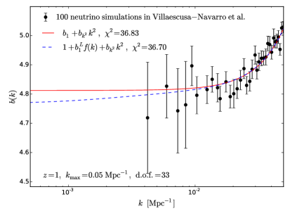
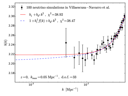
Fig. 18 shows the results at $z=1$ (left) and 0 (right). The data point show the mean of the measurement from 100 realizations with the error on the mean, and the red solid and blue dashed lines show the two models correspondingly. There are 35 data points with two fitting parameters, so the number of degrees of freedom (d.o.f.) is 33. The $\chi^{2}$ values from fitting the mean of the clustering bias to the models are shown in the legend. First we find that the reduced $\chi^{2}$ is close to unity, indicating that the models describe simulations results well. More importantly, we find that the $\chi^{2}$ values between the two models are close, implying that the simulations do not have enough statistical power to distinguish one from another. Namely, both scale-independent and scale-dependent linear bias models are equally consistent with the simulations.

There are two main reasons that the simulations cannot distinguish the two models. First, the scale dependence we predict is on large scale, and even the fundamental mode of the simulation box of $1~{}h^{-1}~{}{\rm Gpc}$ cannot probe the full effect. This can clearly be seen in Fig. 18: at $k\gtrsim 0.01~{}{\rm Mpc}^{-1}$ the two models are almost identical. Note that the large-scale difference between the two bias models will approach to a constant because the response becomes scale independent when $k\ll k_{\rm fs}$. Therefore, to probe this effect we need simulations with box size of a few Gpc. Second, people usually increase $f_{\nu}$ by increasing the neutrino mass instead of number. For larger neutrino mass, the free-streaming length approach to nonlinear scale, so it is challenging to separate the scale-dependent linear bias and nonlinear bias. Moreover, the neutrino clustering becomes important for larger neutrino mass, hence the approximation breaks down and our prediction is invalid. Therefore, an ideal set of simulations to detect this effect is to have a few Gpc box size and $0.05~{}{\rm eV}$ of massive neutrinos mass with $f_{\nu}=5-10\%$. This study is beyond the scope of this paper and is work in progress.

References

- Ahmad et al. (2002) Q. R. Ahmad et al. (SNO), Phys. Rev. Lett. 89, 011301 (2002), arXiv:nucl-ex/0204008 [nucl-ex] .
- Fukuda et al. (2002) S. Fukuda et al. (Super-Kamiokande), Phys. Lett. B539, 179 (2002), arXiv:hep-ex/0205075 [hep-ex] .
- Altmann et al. (2005) M. Altmann et al. (GNO), Phys. Lett. B616, 174 (2005), arXiv:hep-ex/0504037 [hep-ex] .
- Abdurashitov et al. (2002) J. N. Abdurashitov et al. (SAGE), J. Exp. Theor. Phys. 95, 181 (2002), [Zh. Eksp. Teor. Fiz.122,211(2002)], arXiv:astro-ph/0204245 [astro-ph] .
- Fukuda et al. (1998) Y. Fukuda et al. (Super-Kamiokande), Phys. Rev. Lett. 81, 1562 (1998), arXiv:hep-ex/9807003 [hep-ex] .
- Ashie et al. (2005) Y. Ashie et al. (Super-Kamiokande), Phys. Rev. D71, 112005 (2005), arXiv:hep-ex/0501064 [hep-ex] .
- Sanchez et al. (2003) M. C. Sanchez et al. (Soudan 2), Phys. Rev. D68, 113004 (2003), arXiv:hep-ex/0307069 [hep-ex] .
- Henderson et al. (2016) S. W. Henderson et al., Proceedings, 16th International Workshop on Low Temperature Detectors (LTD 16): Grenoble, France, July 20-24, 2015, J. Low. Temp. Phys. 184, 772 (2016), arXiv:1510.02809 [astro-ph.IM] .
- Benson et al. (2014) B. A. Benson et al. (SPT-3G), Proceedings, SPIE Astronomical Telescopes + Instrumentation 2014: Millimeter, Submillimeter, and Far-Infrared Detectors and Instrumentation for Astronomy VII: Montreal, Quebec, Canada, June 24-27, 2014, Proc. SPIE Int. Soc. Opt. Eng. 9153, 91531P (2014), arXiv:1407.2973 [astro-ph.IM] .
- Abazajian et al. (2016) K. N. Abazajian et al. (CMB-S4), (2016), arXiv:1610.02743 [astro-ph.CO] .
- Aghamousa et al. (2016) A. Aghamousa et al. (DESI), (2016), arXiv:1611.00036 [astro-ph.IM] .
- Ellis et al. (2014) R. Ellis et al. (PFS Team), Publ. Astron. Soc. Jap. 66, R1 (2014), arXiv:1206.0737 [astro-ph.CO] .
- Abate et al. (2012) A. Abate et al. (LSST Dark Energy Science), (2012), arXiv:1211.0310 [astro-ph.CO] .
- Spergel et al. (2015) D. Spergel et al., (2015), arXiv:1503.03757 [astro-ph.IM] .
- Laureijs et al. (2011) R. Laureijs et al. (EUCLID), (2011), arXiv:1110.3193 [astro-ph.CO] .
- Lesgourgues and Pastor (2006) J. Lesgourgues and S. Pastor, Phys. Rept. 429, 307 (2006), arXiv:astro-ph/0603494 [astro-ph] .
- Wong (2011) Y. Y. Y. Wong, Ann. Rev. Nucl. Part. Sci. 61, 69 (2011), arXiv:1111.1436 [astro-ph.CO] .
- Hu and Eisenstein (1998) W. Hu and D. J. Eisenstein, Astrophys. J. 498, 497 (1998), arXiv:astro-ph/9710216 [astro-ph] .
- Eisenstein and Hu (1997) D. J. Eisenstein and W. Hu, Astrophys. J. 511, 5 (1997), arXiv:astro-ph/9710252 [astro-ph] .
- LoVerde (2014a) M. LoVerde, Phys. Rev. D90, 083530 (2014a), arXiv:1405.4855 [astro-ph.CO] .
- Shoji and Komatsu (2010) M. Shoji and E. Komatsu, Phys. Rev. D81, 123516 (2010), [Erratum: Phys. Rev.D82,089901(2010)], arXiv:1003.0942 [astro-ph.CO] .
- Blas et al. (2014) D. Blas, M. Garny, T. Konstandin, and J. Lesgourgues, JCAP 1411, 039 (2014), arXiv:1408.2995 [astro-ph.CO] .
- Führer and Wong (2015) F. Führer and Y. Y. Y. Wong, JCAP 1503, 046 (2015), arXiv:1412.2764 [astro-ph.CO] .
- Dupuy and Bernardeau (2015) H. Dupuy and F. Bernardeau, JCAP 1508, 053 (2015), arXiv:1503.05707 [astro-ph.CO] .
- Archidiacono and Hannestad (2016) M. Archidiacono and S. Hannestad, JCAP 1606, 018 (2016), arXiv:1510.02907 [astro-ph.CO] .
- Levi and Vlah (2016) M. Levi and Z. Vlah, (2016), arXiv:1605.09417 [astro-ph.CO] .
- Inman and Pen (2017) D. Inman and U.-L. Pen, Phys. Rev. D95, 063535 (2017), arXiv:1609.09469 [astro-ph.CO] .
- Bird et al. (2012) S. Bird, M. Viel, and M. G. Haehnelt, Mon. Not. Roy. Astron. Soc. 420, 2551 (2012), arXiv:1109.4416 [astro-ph.CO] .
- Hannestad et al. (2012) S. Hannestad, T. Haugbolle, and C. Schultz, JCAP 1202, 045 (2012), arXiv:1110.1257 [astro-ph.CO] .
- Wagner et al. (2012) C. Wagner, L. Verde, and R. Jimenez, Astrophys. J. 752, L31 (2012), arXiv:1203.5342 [astro-ph.CO] .
- Villaescusa-Navarro et al. (2013) F. Villaescusa-Navarro, S. Bird, C. Pena-Garay, and M. Viel, JCAP 1303, 019 (2013), arXiv:1212.4855 [astro-ph.CO] .
- Villaescusa-Navarro et al. (2014) F. Villaescusa-Navarro, F. Marulli, M. Viel, E. Branchini, E. Castorina, E. Sefusatti, and S. Saito, JCAP 1403, 011 (2014), arXiv:1311.0866 [astro-ph.CO] .
- Castorina et al. (2014) E. Castorina, E. Sefusatti, R. K. Sheth, F. Villaescusa-Navarro, and M. Viel, JCAP 1402, 049 (2014), arXiv:1311.1212 [astro-ph.CO] .
- Costanzi et al. (2013) M. Costanzi, F. Villaescusa-Navarro, M. Viel, J.-Q. Xia, S. Borgani, E. Castorina, and E. Sefusatti, JCAP 1312, 012 (2013), arXiv:1311.1514 [astro-ph.CO] .
- Castorina et al. (2015) E. Castorina, C. Carbone, J. Bel, E. Sefusatti, and K. Dolag, JCAP 1507, 043 (2015), arXiv:1505.07148 [astro-ph.CO] .
- Agarwal and Feldman (2011) S. Agarwal and H. A. Feldman, Mon. Not. Roy. Astron. Soc. 410, 1647 (2011), arXiv:1006.0689 [astro-ph.CO] .
- Heitmann et al. (2016) K. Heitmann et al., Astrophys. J. 820, 108 (2016), arXiv:1508.02654 [astro-ph.CO] .
- Inman et al. (2015) D. Inman, J. D. Emberson, U.-L. Pen, A. Farchi, H.-R. Yu, and J. Harnois-Déraps, Phys. Rev. D92, 023502 (2015), arXiv:1503.07480 [astro-ph.CO] .
- Yu et al. (2016) H.-R. Yu et al., (2016), arXiv:1609.08968 [astro-ph.CO] .
- Emberson et al. (2016) J. D. Emberson et al., (2016), arXiv:1611.01545 [astro-ph.CO] .
- Brandbyge and Hannestad (2010) J. Brandbyge and S. Hannestad, JCAP 1001, 021 (2010), arXiv:0908.1969 [astro-ph.CO] .
- Ali-Haimoud and Bird (2012) Y. Ali-Haimoud and S. Bird, Mon. Not. Roy. Astron. Soc. 428, 3375 (2012), arXiv:1209.0461 [astro-ph.CO] .
- Banerjee and Dalal (2016) A. Banerjee and N. Dalal, JCAP 1611, 015 (2016), arXiv:1606.06167 [astro-ph.CO] .
- McDonald (2003) P. McDonald, Astrophys. J. 585, 34 (2003), arXiv:astro-ph/0108064 [astro-ph] .
- Sirko (2005) E. Sirko, Astrophys. J. 634, 728 (2005), arXiv:astro-ph/0503106 [astro-ph] .
- Gnedin et al. (2011) N. Y. Gnedin, A. V. Kravtsov, and D. H. Rudd, Astrophys. J. Suppl. 194, 46 (2011), arXiv:1104.1428 [astro-ph.CO] .
- Li et al. (2014) Y. Li, W. Hu, and M. Takada, Phys. Rev. D89, 083519 (2014), arXiv:1401.0385 [astro-ph.CO] .
- Wagner et al. (2015a) C. Wagner, F. Schmidt, C.-T. Chiang, and E. Komatsu, Mon. Not. Roy. Astron. Soc. 448, L11 (2015a), arXiv:1409.6294 [astro-ph.CO] .
- Barreira and Schmidt (2017a) A. Barreira and F. Schmidt, (2017a), arXiv:1705.01092 [astro-ph.CO] .
- Wagner et al. (2015b) C. Wagner, F. Schmidt, C.-T. Chiang, and E. Komatsu, JCAP 1508, 042 (2015b), arXiv:1503.03487 [astro-ph.CO] .
- Barreira and Schmidt (2017b) A. Barreira and F. Schmidt, JCAP 1706, 053 (2017b), arXiv:1703.09212 [astro-ph.CO] .
- Li et al. (2016) Y. Li, W. Hu, and M. Takada, Phys. Rev. D93, 063507 (2016), arXiv:1511.01454 [astro-ph.CO] .
- Lazeyras et al. (2016) T. Lazeyras, C. Wagner, T. Baldauf, and F. Schmidt, JCAP 1602, 018 (2016), arXiv:1511.01096 [astro-ph.CO] .
- Baldauf et al. (2016) T. Baldauf, U. Seljak, L. Senatore, and M. Zaldarriaga, JCAP 1609, 007 (2016), arXiv:1511.01465 [astro-ph.CO] .
- Cieplak and Slosar (2016) A. M. Cieplak and A. Slosar, JCAP 1603, 016 (2016), arXiv:1509.07875 [astro-ph.CO] .
- Chiang et al. (2017) C.-T. Chiang, A. M. Cieplak, F. Schmidt, and A. Slosar, (2017), arXiv:1701.03375 [astro-ph.CO] .
- Chiang and Slosar (2017) C.-T. Chiang and A. Slosar, (2017), arXiv:1708.07512 [astro-ph.CO] .
- Dai et al. (2015) L. Dai, E. Pajer, and F. Schmidt, JCAP 1510, 059 (2015), arXiv:1504.00351 [astro-ph.CO] .
- Hu et al. (2016) W. Hu, C.-T. Chiang, Y. Li, and M. LoVerde, Phys. Rev. D94, 023002 (2016), arXiv:1605.01412 [astro-ph.CO] .
- Hu and Joyce (2017) W. Hu and A. Joyce, Phys. Rev. D95, 043529 (2017), arXiv:1612.02454 [astro-ph.CO] .
- Chiang et al. (2016) C.-T. Chiang, Y. Li, W. Hu, and M. LoVerde, Phys. Rev. D94, 123502 (2016), arXiv:1609.01701 [astro-ph.CO] .
- Chiang et al. (2014) C.-T. Chiang, C. Wagner, F. Schmidt, and E. Komatsu, JCAP 1405, 048 (2014), arXiv:1403.3411 [astro-ph.CO] .
- Chiang et al. (2015) C.-T. Chiang, C. Wagner, A. G. Sánchez, F. Schmidt, and E. Komatsu, JCAP 1509, 028 (2015), arXiv:1504.03322 [astro-ph.CO] .
- Blas et al. (2011) D. Blas, J. Lesgourgues, and T. Tram, JCAP 1107, 034 (2011), arXiv:1104.2933 [astro-ph.CO] .
- Lesgourgues and Tram (2011) J. Lesgourgues and T. Tram, JCAP 1109, 032 (2011), arXiv:1104.2935 [astro-ph.CO] .
- Hu and Sugiyama (1996) W. Hu and N. Sugiyama, Astrophys. J. 471, 542 (1996), arXiv:astro-ph/9510117 [astro-ph] .
- Crocce et al. (2006) M. Crocce, S. Pueblas, and R. Scoccimarro, Mon. Not. Roy. Astron. Soc. 373, 369 (2006), arXiv:astro-ph/0606505 [astro-ph] .
- Springel (2005) V. Springel, Mon. Not. Roy. Astron. Soc. 364, 1105 (2005), arXiv:astro-ph/0505010 [astro-ph] .
- Gill et al. (2004) S. P. D. Gill, A. Knebe, and B. K. Gibson, Mon. Not. Roy. Astron. Soc. 351, 399 (2004), arXiv:astro-ph/0404258 [astro-ph] .
- Knollmann and Knebe (2009) S. R. Knollmann and A. Knebe, Astrophys. J. Suppl. 182, 608 (2009), arXiv:0904.3662 [astro-ph.CO] .
- (71) “FFTW,” http://www.fftw.org.
- Jeong and Komatsu (2006) D. Jeong and E. Komatsu, Astrophys. J. 651, 619 (2006), arXiv:astro-ph/0604075 [astro-ph] .
- LoVerde (2014b) M. LoVerde, Phys. Rev. D90, 083518 (2014b), arXiv:1405.4858 [astro-ph.CO] .
- Hui and Parfrey (2008) L. Hui and K. P. Parfrey, Phys. Rev. D77, 043527 (2008), arXiv:0712.1162 [astro-ph] .
- Parfrey et al. (2011) K. Parfrey, L. Hui, and R. K. Sheth, Phys. Rev. D83, 063511 (2011), arXiv:1012.1335 [astro-ph.CO] .
- Senatore (2015) L. Senatore, JCAP 1511, 007 (2015), arXiv:1406.7843 [astro-ph.CO] .
- Marin (2011) F. Marin, Astrophys. J. 737, 97 (2011), arXiv:1011.4530 [astro-ph.CO] .
- Gil-Marín et al. (2015) H. Gil-Marín, J. Noreña, L. Verde, W. J. Percival, C. Wagner, M. Manera, and D. P. Schneider, Mon. Not. Roy. Astron. Soc. 451, 539 (2015), arXiv:1407.5668 [astro-ph.CO] .
- Eftekharzadeh et al. (2015) S. Eftekharzadeh, A. D. Myers, M. White, D. H. Weinberg, D. P. Schneider, Y. Shen, A. Font-Ribera, N. P. Ross, I. Paris, and A. Streblyanska, Mon. Not. Roy. Astron. Soc. 453, 2779 (2015), arXiv:1507.08380 [astro-ph.CO] .
- Hu et al. (1998) W. Hu, D. J. Eisenstein, and M. Tegmark, Phys. Rev. Lett. 80, 5255 (1998), arXiv:astro-ph/9712057 [astro-ph] .
- Chiang (2017) C.-T. Chiang, Phys. Rev. D95, 123517 (2017), arXiv:1701.03374 [astro-ph.CO] .
- LoVerde (2016) M. LoVerde, Phys. Rev. D93, 103526 (2016), arXiv:1602.08108 [astro-ph.CO] .
- Senatore and Zaldarriaga (2017) L. Senatore and M. Zaldarriaga, (2017), arXiv:1707.04698 [astro-ph.CO] .
- Villaescusa-Navarro et al. (2017) F. Villaescusa-Navarro, A. Banerjee, N. Dalal, E. Castorina, R. Scoccimarro, R. Angulo, and D. N. Spergel, (2017), arXiv:1708.01154 [astro-ph.CO] .
- Scoccimarro (1998) R. Scoccimarro, Mon. Not. Roy. Astron. Soc. 299, 1097 (1998), arXiv:astro-ph/9711187 [astro-ph] .
- Bouchet et al. (1995) F. R. Bouchet, S. Colombi, E. Hivon, and R. Juszkiewicz, Astron. Astrophys. 296, 575 (1995), arXiv:astro-ph/9406013 [astro-ph] .
- Navarro et al. (1997) J. F. Navarro, C. S. Frenk, and S. D. M. White, Astrophys. J. 490, 493 (1997), arXiv:astro-ph/9611107 [astro-ph] .
- LoVerde and Zaldarriaga (2014) M. LoVerde and M. Zaldarriaga, Phys. Rev. D89, 063502 (2014), arXiv:1310.6459 [astro-ph.CO] .
- Davis et al. (1985) M. Davis, G. Efstathiou, C. S. Frenk, and S. D. M. White, Astrophys. J. 292, 371 (1985).
- Assassi et al. (2014) V. Assassi, D. Baumann, D. Green, and M. Zaldarriaga, JCAP 1408, 056 (2014), arXiv:1402.5916 [astro-ph.CO] .