Topological critical slowing down:
variations on a toy model
Abstract
Numerical simulations of lattice quantum field theories whose continuum counterparts possess classical solutions with non-trivial topology face a severe critical slowing down as the continuum limit is approached. Standard Monte-Carlo algorithms develop a loss of ergodicity, with the system remaining frozen in configurations with fixed topology. We analyze the problem in a simple toy model, consisting of the path integral formulation of a quantum mechanical particle constrained to move on a circumference. More specifically, we implement for this toy model various techniques which have been proposed to solve or alleviate the problem for more complex systems, like non-abelian gauge theories, and compare them both in the regime of low temperature and in that of very high temperature. Among the various techniques, we consider also a new algorithm which completely solves the freezing problem, but unfortunately is specifically tailored for this particular model and not easily exportable to more complex systems.
I Introduction
Numerical Monte-Carlo simulations of lattice gauge theories are currently one of the most important tools for the non-perturbative study of quantum field theories for fundamental interactions and condensed matter systems. The general idea of the method is to reduce the computation of the path integral to the sampling of a finite dimensional probability distribution, a task that can be performed through Markov chain Monte-Carlo (MCMC).
In some cases, some hard problems are found which prevent a full exploitation of numerical simulations. A particularly severe problem that is sometimes encountered is the loss of the positivity of the probability distribution, a fact generically indicated as “sign problem”. This happens for the cases of QCD at finite baryon density or in the presence of a term and in many condensed matter models Aarts (2016); Loh et al. (1990); Troyer and Wiese (2005). In some other cases the problem is simply the presence of long autocorrelation times, related to some particular slow modes, leading eventually to a loss of ergodicity and thus to a breakdown of the algorithm. Such a behaviour is common to many complex systems and it appears, for instance, close to a phase transition Berg (2004); Newman and Barkema (2001).
A well known problem of the second type is related to the presence of classical solutions with non-trivial topology. In the continuum, the space of field configurations contributing to the path integral divides in homotopy classes, each class being characterized by the value of a topological invariant taking only discrete (typically integer) values. On a discrete space-time the concept of homotopy, which strictly speaking is lost, is recovered as the continuum limit is approached. Since the typical MCMC algorithms move in the configuration space in an approximately continuous way, close to the continuum they become completely unable to change the topology of the field.
This problem severely affects the study of -dependence in QCD Alles et al. (1996); Schaefer et al. (2011); Bonati et al. (2016a) and in many QCD-like models Campostrini et al. (1992); Del Debbio et al. (2002, 2004); Flynn et al. , the most relevant case being the study of the axion potential at finite temperature Berkowitz et al. (2015); Borsanyi et al. (2016a); Kitano and Yamada (2015); Trunin et al. (2016); Bonati et al. (2016a); Petreczky et al. (2016); Frison et al. (2016); Borsanyi et al. (2016b). Several methods and new algorithms have been proposed to solve or at least alleviate this problem, however no comparative investigation of the efficiency of these proposals exists in the literature so far. The purpose of this study is to make a critical comparison of the various techniques in one of the simplest model where an analogous problem appears: the numerical simulation of the thermal path integral of a quantum particle constrained to move on a circumference; we will consider both the free case and the case in which a potential is present (quantum pendulum).
The use of such a simple model will enable us to extract the autocorrelation time of the topological susceptibility for several values of the lattice spacing and to study its critical behaviour as the continuum limit is approached. This behaviour (e.g. exponential or power-law in ) is expected to be characteristic of the updating scheme, independently of the specific model adopted as far as topologically stable classical solutions exist. Let us stress that, instead, the prefactor in front of the leading -dependence, which eventually fixes what is the best algorithm to be chosen for a given value of , is likely dependent on the chosen model. However our main focus here is on the approach to the continuum limit: that is pre-factor independent and contains relevant information which is expected to be model independent.
We will show that all methods proposed so far to sample the configuration space present some residual critical slowing down as the continuum limit is approached, even if some of them reduce autocorrelation times by several orders of magnitude with respect to standard local algorithms. We will also present a new algorithm, which is based on the idea that the correct way to deal with the problem is to invent some non-local move in configuration space, capable of jumping directly from one topological sector into another one. Such a move can be easily found in the simple model studied in this paper and completely kills the critical slowing down of the topological modes. The basic idea of this update scheme seems to be applicable also to more interesting theories, like 4d non-abelian gauge theories, however its actual implementation requires further studies to overcome some technical difficulties.
The paper is organized as follows: in Sec. II we introduce the model and we review some basic facts about the dependence, while in Sec. III the discretization to be used in the simulations is described. With Sec. IV.1 we start the analysis of the different algorithms that can be used to numerically investigate the topological properties of the model at , providing results for the autocorrelation times obtained by using the different approaches (standard Metropolis, tailor method, slab method, open boundary conditions, parallel tempering). In Sec. IV.6 we study instead the high-temperature limit of the model, that presents peculiar difficulties. Finally in Sec. V we present our conclusions.
II The model and some of its properties
The fact that a simple unidimensional quantum mechanical model can have some common features with four-dimensional non-abelian gauge theories can be at a first sight quite surprising, however (as far as the dependence is concerned) what matters is topology: for a quantum particle moving on the circumference, the topology of the configuration space, ; for a 4d non-abelian quantum field theory, the topology of the gauge group, .
Let us consider the case first; here and in the following we set . The thermal partition function of a quantum free particle of mass , moving along a circumference of radius at temperature , can be written as a sum over energy (angular momentum) eigenstates
| (1) |
while in the path integral approach
| (2) | ||||
where is the Euclidean action, the path integral extends over periodic paths, , and is characterized by the fact that only continuous paths, even if not differentiable, contribute to it. For that reason, analogously to what happens for the configurations contributing to the path integral of non-abelian gauge theories, paths divide in homotopy classes (topological sectors), classified by a topological number , which corresponds to the number of times the path winds around the circumference while winding around the Euclidean time circle.
Further insight in the origin of these common features, including the introduction of the parameter, is obtained by means of the canonical quantization approach Jackiw (1980); Treiman et al. (1985). The Hamiltonian of a quantum particle moving on a circumference commutes with the unitary operator that implements the translation , where is the angle that parametrizes the position on the circumference. As a consequence we can use a base of common eigenvectors of and and restrict ourselves to the subspace corresponding to the eigenvalue of . The same argument can be applied to the case of 4d non-abelian gauge theories: local gauge invariance, in the form of the Gauss law, implies that local gauge transformations act trivially on the whole Hilbert space, but the theory is invariant also under transformations having nontrivial behaviour at infinity. The operator that implements these “large” gauge transformations is the analogous of the operator in the quantum mechanics example (for more details see, e.g., Ref. Smilga (2001); Strocchi (2013)).
To see that the restriction to the -sector of the Hilbert space is equivalent to the introduction of a -term in the Lagrangian it is convenient to use the path integral formulation. We can use the identity to fix the constraint , thus obtaining
| (3) | ||||
where is the original unconstrained Lagrangian.
The restriction can be interpreted also as a modification of the properties of the physical states for translations , i.e. from standard periodic boundary conditions (b.c.) to b.c. which are periodic up to a phase factor . There are various ways to realize that in practice. If the particle has an electric charge , the introduction of a magnetic flux piercing the circle is equivalent to the introduction of a non-zero . The same happens when considering a reference frame rotating around the axis of the circumference with angular velocity (see e.g Krauth (2006)). It should be noted that, analogously to what happens in non-abelian gauge theories, a non-zero term modifies the Lagrangian by adding a total derivative to it, therefore it is completely irrelevant at the classical level, and only plays a role at the quantum level because of the non-trivial topology of the configuration space.
In order to simplify the notation we introduce the variable defined by and in the following we will use a system of units such that . With these conventions the Hamiltonian operator can be written as
| (4) |
where , is a function of period and the wave function satisfies the boundary conditions ; the corresponding Lagrangian is
| (5) |
The partition function can be rewritten in the path integral formalism by means of the Euclidean Lagrangian as ()
| (6) |
where the functional integration extends over all functions (with the extrema and identified) satisfying the boundary condition and the Euclidean Lagrangian is given by
| (7) |
Note that the term becomes imaginary after the analytical continuation to Euclidean time, because it involves a total time derivative; this will have important consequences in the following.
Also for generic values of only continuous trajectories have a non-vanishing weight in the integral, so that paths can be grouped into homotopy classes labelled by the number of times a path winds around the circumference while winding once around the Euclidean time. The integral can thus be decomposed into a sum over the different topologies and an integration over quantum fluctuations in each fixed topological sector. As usual in the context of the semiclassical approximation (see, e.g., Ref. Coleman (1988)), it is convenient to select as representatives of the homotopy classes the paths having the smaller values of the Euclidean action, that correspond to the solutions of the Euclidean equations of motions.
This model presents some interesting features even in the non-interacting limit : in this case the partition function at temperature is given in the Hamiltonian formalism by
| (8) |
The solution of the Euclidean equation of motion having winding number is
| (9) |
and the corresponding Euclidean action determines the semiclassical exponential weight of the configuration in the partition function ( is the exponent in Eq. (10)). When the action is quadratic in the field the semiclassical approximation is in fact exact, the integral over the fluctuations at fixed topology is Gaussian and gives a prefactor of the form , so that we finally obtain from the Lagrangian formalism
| (10) |
which could have been also obtained directly from Eq. (8) by using the Poisson summation formula. Eq. (10) gives a dual representation of the partition function in Eq. (8), in which the high and low limit are exchanged. Indeed, in Eq. (8) only a few terms of the sum are relevant at low , while at high all terms contribute and the sum can be changed into an integral, exactly the opposite happens in the sum over topological sectors in Eq. (10).
From the partition function we can obtain the free energy density
| (11) |
that encodes the dependence of the theory. Although for the model studied in this paper and there is no need to differentiate between intensive and extensive quantities, we will use the intensive lower-case letters to conform to standard notations. Two properties of the free energy density that are evident in the non-interacting case but are true also in more general cases are the following:
-
•
;
-
•
.
It is simple to show that the first property is valid if the potential appearing in the Lagrangian Eq. (5) satisfies (i.e. if is parity invariant): it is sufficient to perform in the path-integral the change of variable and realize that this corresponds to the substitution in the action. That is a simple consequence of the fact that in Euclidean time the term becomes imaginary (see Eq. (7)): the complex exponential induces cancellations in the path-integral expression of the partition function and thus ; a fact that, when the term is interpreted in terms of a non-zero magnetic flux, is equivalent to a diamagnetic behavior for the charged particle on the circumference. Both these properties remain true also in the case of 4d non-abelian gauge theories and the proof is basically the same; the fact that the free energy has a minimum at is related to the Vafa-Witten theorem Vafa and Witten (1984) and it is at the basis of the Peccei-Quinn solution of the strong CP problem Peccei and Quinn (1977a, b).
For generic values, the free energy density cannot be written in closed form using elementary transcendental functions even for the non-interacting case111In fact it can be written in terms of the Jacobi function and the relation between Eqs. (8),(10) in nothing but the fundamental functional equation for Bellman (2013); Whittaker and Watson (1996)., however there are two notable limits in which this is possible: the very low and very high temperature cases. In the extreme low temperature regime we see from Eq. (8) that for each value only a single eigenstate contributes and we obtain the expression
| (12) |
that is singular at , where a crossing of two energy levels happens. Large arguments suggest such a multi-branched -dependence to be present also in 4d Yang-Mills theories at zero temperature Witten (1980, 1998), with a spontaneous breaking of the CP symmetry taking place at Gaiotto et al. (2017); the singularity at is present also in QCD for some values of the quark masses Di Vecchia and Veneziano (1980); Gaiotto et al. ; Di Vecchia et al. (2017).
In the opposite limit, using Eq. (10) we see that only the modes with have non-negligible contribution to the dependence and we obtain
| (13) |
Such an expression is reminiscent of the Dilute Instanton Gas Approximation in the high temperature phase of 4d non-abelian gauge theories Gross et al. (1981), however the underlying physics is different, basically because an underlying spatial volume which diverges in the thermodynamic limit is missing in the simple 1D model. In the present model the term is a consequence of the fact that at most a single “instanton” is present, while in the 4d case it is a consequence of the fact that instantons are almost independent of each other at high temperature. This makes the system behave “as if” a single instanton were present, although an increasingly large number of them is in fact present as the thermodynamic limit is approached.
A parametrization that is commonly used to describe the -dependence of the free energy density in the general case is Vicari and Panagopoulos (2009)
| (14) |
where is the so-called topological susceptibility and the coefficients parametrize higher order terms in . As previously noted, in the Euclidean path-integral formulation the -term in the Lagrangian becomes imaginary; this implies that simulations cannot be performed directly at non-vanishing real values because of a sign problem that hinders the applicability of standard importance sampling MCMC.
The most commonly used method to compute the coefficients and appearing in Eq. (14) is thus to write them in terms of expectation values computed at : it is indeed easy to verify that the first few terms are given by
| (15) |
and in general is proportional to the -th cumulant of the winding number distribution at . From Eqs. (12)-(13) we can see that for the low and high temperature regimes of the non-interacting theory we have respectively
| (16) | ||||
A different approach that can be used to extract these coefficients is to perform simulations at imaginary values of the parameter (analytic continuation method Azcoiti et al. (2002); Alles and Papa (2008); Alles et al. (2014); Panagopoulos and Vicari (2011); D’Elia and Negro (2012, 2013); Bonati et al. (2016b, c)). Although this approach presents some technical advantages with respect to the Taylor expansion method, the observed critical slowing down close to the continuum limit is the same in both approaches, so in this paper we will concentrate just on simulations performed at .
III Discretization
The first step to be accomplished in order to perform numerical simulations of a model by using path-integral techniques is to write down the discretized form of the Euclidean action. For the case of the Lagrangian Eq. (7) this is quite a simple task, since it is sufficient to use finite differences instead of derivatives. The only subtlety stems from the fact that the theory is defined on a circumference, thus an ambiguity is present in the definition of the distance between two points. In order to resolve this ambiguity we introduce the following definition of distance (with sign) on the circumference of length 1, that correspond to the oriented shortest path between and :
| (17) |
With this definition the discretized Euclidean action can be written in the form
| (18) | ||||
where , , is the lattice spacing in the temporal direction222Notice that is a dimensionless parameter. Indeed, without fixing and we would have obtained in place of , which is the dimensionless ratio between the lattice spacing and the typical time scale of the quantum system. Therefore, with the chosen units, means that the discretization scale is much smaller than the physical time scale. and we will almost always use the thermal boundary conditions . The last term in Eq. (18) is the discretizaton of the winding number , that in this simple system takes integer values also at non-vanishing lattice spacing333Without the proper definition of distance given in Eq. (17), the discretized topological charge appearing in Eq. (18) would be strictly zero. (contrary to what happens in 4d gauge theories, see, e.g., Ref. Vicari and Panagopoulos (2009)). In the following we will study the system at with the potential
| (19) |
that for reduces to the non-interacting case, and we will be mainly interested in the integrated autocorrelation time of the topological susceptibility, that will be denoted simply by . Another parameter that is fundamental in order to asses the efficiency of the update methods is obviously the CPU-time required to perform a single update step. However, for the quantum particle moving on a circumference, the computational complexity of the various update schemes investigated is practically the same, with some caution needed only for the cases of open boundary conditions and parallel tempering, as will be discussed later on.
In order to estimate integrated autocorrelation times several procedures exist. The standard way, stemming from its very definition, is to directly integrate the autocorrelation function:
| (20) |
where is a generic primary observable and and denote two generic draws of the observable taken along the Monte-Carlo simulation at Markov chain steps apart from each other. The numerical computation of this sum requires some care and standard methods exist to optimize the integration range, in order to minimize the final error Madras and Sokal (1988); Wolff (2004). We used the Python implementation described in De Palma et al. , that is freely available under the MIT License.
However, probably the most straightforward and practical procedure is to use the relation Berg (2004); Muller-Krumbhaar and Binder (1973)
| (21) |
where is the correct standard error for estimated by properly taking into account autocorrelations, is the size of the sample, and is the naive standard error computed without taking autocorrelations into account. To use this expression we need the value of , that can be computed using standard blocking and resampling procedures (see, e.g., Ref. Berg (2004); Newman and Barkema (2001)). In all the cases in which both methods were applicable, we verified that the autocorrelation times estimated by using the two procedures were compatible with each other444Some caution is however needed in the choice of the parameter that enters the automatic windowing procedure of Wolff (2004): this parameter is typically set to but in some cases it was necessary to use values up to for the integral of the autocorrelation function to reach a plateau around the point automatically chosen by the algorithm (for a different approach to this problem see Schaefer et al. (2011)).. Moreover in all the cases we used time-histories long at least for the largest values of the autocorrelation time.
In the following section we will describe the results obtained for the autocorrelation time of the topological susceptibility using different algorithms. In all these sections, apart from Sec. IV.6, we will consider the low temperature regime of the theory, fixing the temporal extent of the lattice to the value . This corresponds to a temperature , which for and in the chosen units corresponds to , where is the energy gap between the ground state and the first excited state of the free system, so that is indeed quite small. We verified to be deep in the low temperature region for all the values of the parameter used in our simulations.
IV Comparison of different approaches
IV.1 Variation 1: Standard Metropolis
The first adopted algorithm was the standard Metropolis one Metropolis et al. (1953): we used a 5 hit scheme, with sites updated in lexicographic order and the proposed update being of the form
| (22) |
where is a random number and is a parameter.
By increasing the value of larger variations are proposed, that could help in reducing autocorrelations, however large values of have smaller acceptance rates. In order to investigate the continuum limit of the autocorrelation time we have to fix the dependence of the parameter on the lattice spacing . Given the form of the action in Eq. (18) it is natural to guess that using the acceptance rate will be constant as Creutz and Freedman (1981), and this is indeed what we numerically found. This is however not a priori the optimal choice if our aim is to reduce the autocorrelation of the topological susceptibility. From some test runs we concluded that the dependence of on is practically negligible and that large values of correspond to significantly smaller autocorrelation times, despite the fact that the acceptance rate is smaller. For this reason we decided to fix the value in our simulation for all the lattice spacings studied.
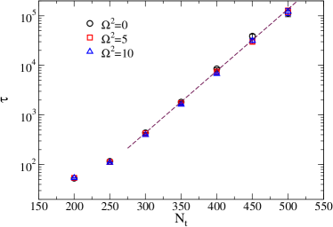
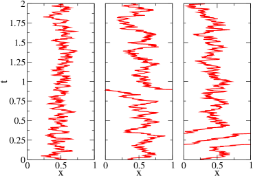
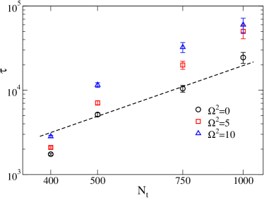
In Fig. 1 we display the scaling of the autocorrelation time of the topological susceptibility as a function of the inverse of the lattice spacing (remember that ) for simulations performed using Metropolis updates with . The autocorrelation time is well described by an exponential function in , which is consistent with the results obtained in models Campostrini et al. (1992); Flynn et al. , Yang-Mills theories Del Debbio et al. (2002, 2004) and QCD Alles et al. (1996); Schaefer et al. (2011); Bonati et al. (2016a). The critical slowing down of the winding number emerges, as one approaches the continuum limit, because for very small lattice spacing the local updates effectively become continuum diffusive processes. However, in order to change the value of the winding number by such a type of process, one necessarily has to go across paths (or configurations, in the case of a field theory) developing a discontinuity (a cut) somewhere and thus corresponding to very large values of the action.
Let us discuss this point more in details: some examples of topologically nontrivial paths obtained in our MC simulations are shown in Fig. 2. From these figures it is easy to understand that, in order to change the value of the winding number by a local Metropolis step, it is necessary to accept an update in which two temporally consecutive points become very far apart from each other, i.e. . This is however very unlikely to happen because of the large action of this configuration. From this very simple argument one can guess the exponent of the exponential slowing down shown in Fig. 1 to be given roughly by
| (23) |
which is indeed of the same order of magnitude of the observed value 0.0290(5) (see Fig. 1).
We thus have a consistent picture in which the “barriers” that prevent the changes of the winding number correspond to the very high values of the action of the configurations one is constrained to go through when moving from one topological sector to the other by a local algorithm. Since a shift of the action of each topological sector as a whole does not touch significantly the weights of those unlikely configurations, it does not remove the barriers. As a consequence, it is to be expected that a naive application of the multicanonical update Berg and Neuhaus (1992) or similar approaches (like e.g. metadynamics Laio and Parrinello (2002); Laio and Gervasio (2008)) would not help in removing the critical slowing down, and this is indeed what we observed.
On the other hand the situation for these classes of update schemes seems to be better in field theories where one has to deal with non-integer valued definitions of the winding number in the discretized theory, since a potential based on a real valued charge can make some distinction, at least in principle, between different configurations belonging to the same topological sector. Indeed, very promising results were obtained in Ref. Laio et al. (2016) for 2D models, where the metadynamics was coupled to a discretization of the winding number that is not strictly integer at non-vanishing lattice spacing. Encouraging preliminary results obtained using a conceptually related method, the density of state approach (see e.g. Wang and Landau (2001); Langfeld et al. (2012)), have been recently presented in Cossu et al. (2017).
IV.2 Variation 2: Tailor method
In this section we are going to describe a method that is specifically targeted at reducing the topological slowing down for the quantum particle moving on a circumference. The idea is similar, in some sense, to the one used in cluster updates of spin systems (see, e.g., Ref. Newman and Barkema (2001)), i.e. to make use of non-local updates to improve the decorrelation.
The critical slowing down of the winding number was linked in the previous section to the necessity of passing through discontinuities to change the topology when using a local algorithm. However a non-local update could in principle be able to move from one sector to the other in one single step, by crossing through the barrier in a sort of tunnel effect. To remove the slowing down such a step must be able to connect paths which, while belonging to different topological sectors (typically adjacent ones), have equal or similar actions.
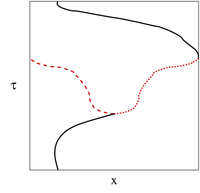
One can likely invent several kinds of step like that. The one we propose here, which is specifically devised for the case, is based on the idea that if we take a piece of a path and modify it in such a way that for each (a reflection around some point will make the job) the action of that piece will remain the same, while its contribution to the winding will change sign. If we can cut away a piece from a starting path, reflect it and sew it back to the uncut part with a minimal loss of continuity in the cut regions, we will be able to make a big step in winding number while leaving the action almost unchanged.
Of course, this sort of path surgery technique will work only for well chosen paths and cut points. In Fig. 3 we show an example which clarifies the conditions: the cut piece of path must wind a half-integer number of times around the circumference, i.e its end points must be diametrically opposite to each other, so that, after reflection, it can be sewed back to the uncut path exactly; that also means that will change by an integer number, by in particular. Because of this underlying pictorial representation, we have named this technique as the “tailor method”.
The above idea can lead to a well defined microcanonical step in the case of continuous paths. We have now to properly implement it in the case of discrete paths, and in a way such that detailed balance is satisfied. More in detail, the algorithm is the following:
-
1.
randomly choose a value , to which the value of the path is associated. Because of the periodic boundary condition in the time direction, up to an irrelevant shift of indices we can assume in the following .
-
2.
Find the first value such that
(24) where is a fixed parameter. If no such point exists abort the update.
-
3.
Propose the update consisting of the change
(25) for all in .
-
4.
Accept or reject the proposed update with a Metropolis test.
It is easy to see that this algorithm satisfies detailed balance and that, when the update is accepted, the winding number is changed by ; moreover, when , the action of the proposed configuration differs from the old one only because of the joint at , so the acceptance probability is expected to be reasonably large, at least in the non-interacting case. Actually, in the continuum limit the acceptance will be exactly one since the algorithm becomes microcanonical (at least for ): in some sense, this kind of update performs at its best right in the continuum limit. Since this algorithms is almost microcanonical it must be obviously used together with other more standard algorithms which can efficiently update the action. Finally we note that the computational burden required for such a non-local update is approximately the same as the one needed to perform a Metropolis sweep for all the points of the lattice.
The algorithm just described could remind the reader of the cluster algorithms defined by embedding discrete Ising-like variable in a continuum model Wolff (1989); Brower and Tamayo (1989) and, in particular, of the cluster algorithm described in Evertz et al. (1991) for the solid on solid model of surface growth; there is however an important difference. The general aim of these cluster algorithms is to perform non-local updates on large scale clusters to reduce the autocorrelation times of local observables. In our case this is not enough and we also have to ensure that during the update the winding number is changed, which is not guaranteed just by the fact that the updated region is macroscopically large. In particular we expect the standard stochastic way of building up the cluster to be less efficient than the deterministic one explained before to decorrelate topological variables.
The tailor algorithm can be extended without change to the case. In this case we expect a loss of performance because of different effects: on one hand, the action of the path will change after the step, because of the potential term, so that the acceptance will diminish; on the other hand, large values of will suppress large scale fluctuations of the path, hence the probability of finding diametrically opposite points. However, in both cases the problem is not related to the microscopic scale, so that the scaling of the performance to the continuum limit is expected to be equally good.
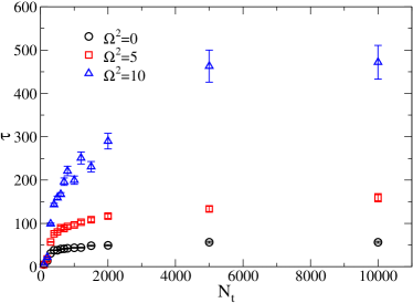
In our implementation we used and a non-local update was proposed every Metropolis updates ( hits with ). The integrated autocorrelation time of the topological susceptibility is reported in units of the elementary updates in Fig. 4, obtained using a statistics of elementary updates (of which were non-local tailor updates), from which we can see that the topological slowing down problem is completely resolved by using the tailor update method. A nontrivial dependence of the autocorrelation time on the parameter is observed, which is easy to understand based on the discussion above. Indeed for the values found for the acceptance of a tailor move have been respectively . However, the good news are that a sort of saturation of the autocorrelation time towards the continuum limit is observed in all cases, independently of the value of .
Given the resolutive nature of this kind of algorithm, it would be a blessing if an analogous one could be found for field theories with a similar problem of autocorrelation of topological modes, like QCD. It is important to stress that for the specific toy model studied in this paper it is surely possible to find other specific algorithms that drastically reduce or completely remove the critical slowing down: given the simplicity of the model it would for example be reasonably simple to implement multilevel/multigrid algorithm like the ones described in Ceperley and Pollock (1986); Goodman and Sokal (1986); Ceperley (1995); Goodman and Sokal (1989), not to mention the possibility of performing the sampling directly in momentum space. However these methods are known since quite long times and their applicability to theories involving gauge degrees of freedom revealed to be very limited. On the contrary, the idea of finding a global field transformation over a region of spacetime which changes the sign of the winding density while leaving the action unchanged is easily extendable: time reversal could for example be used for 4d gauge theories. What is significantly less easy, in higher dimensions, is to be successful in finding the region of space-time which can be cut away and then sewed back after the field transformation, in such a way that it fits almost perfectly with the rest, so that the global action change is negligible. For that reason, while keep thinking about this idea is surely worth doing, let us now turn to more conventional algorithmic improvements, which are more easily extendable to the case of field theories.
IV.3 Variation 3: Slab method
The idea of looking at sub-volumes to estimate the topological susceptibility is around since some time Shuryak and Verbaarschot (1995); de Forcrand et al. (1999) and was recently suggested as a way out of the freezing problem. The basic idea is quite simple and appealing: even if on the whole lattice the winding number does not change, we can look at local fluctuations and try to extract information from them.
The way in which this general idea was applied in Refs. Bietenholz et al. (2015, 2016) is the following: if we know the probability distribution of having a winding number in the volume , we can obtain the probability of having winding number in the volume (with ) when the total winding is frozen to the value as
| (26) |
If we now assume that it can be shown that, when on the whole volume,
| (27) |
and the value of can thus be extracted from sub-volume measurements.
The distribution of the topological charge can be quite often approximated, at least as a first approximation, by a Gaussian behaviour, however this is by no mean guaranteed. The accuracy of this approximation can be quantitatively assessed by looking at the coefficients defined in Eq. (14): since they are proportional to the cumulants of the winding number distribution, they indeed measure how close this distribution is to a Gaussian.
For the case of the quantum particle on a circumference we can see from Eq. (16) that, for the non-interacting case, the distribution is well approximated by a continuum Gaussian in the low temperature regime (it is exactly Gaussian at zero temperature), while this is no more the case in the high temperature regime. Something very similar happens also for 4d Yang-Mills theories and QCD: in the low temperature phase the value of is very small and in fact it goes to zero when the number of color increases Witten (1980, 1998); Di Vecchia and Veneziano (1980); Bonati et al. (2016b, c), in the high temperature phase the same values as in Eq. (16) are expected Gross et al. (1981); Bonati et al. (2013); Bonati (2015); Borsanyi et al. (2016a); Bonati et al. (2016a), that differs significantly from the Gaussian ones.
For the case of the quantum mechanical particle moving on circumference at low temperature, significant non-gaussianities are expected also in the presence of a non-vanishing external potential; for this reason in the following of this section we will restrict to the case , in order to use the simple expression Eq. (27). It seems reasonable that the formalism can be extended to take into account also the first few corrections to non-gaussianity, parametrized, e.g., by and , but we will not pursue this generalization in the present work.
To test the slab method we used lattice spacings small enough that no change of the winding number was expected to happen in the updates accumulated (that in all the cases was also a posteriori verified). For the update we used the same recipe as in the standard Metropolis case, the lattice temporal extent was fixed once again to and results corresponding to the different slab sizes (i.e. ) are completely independent from each other, since they were extracted from independent runs. It should be noted that, while this is not the procedure that would be adopted for computationally more intensive models, our interest here is just in the continuum scaling of the autocorrelation time of topological observables measured at fixed slab size .
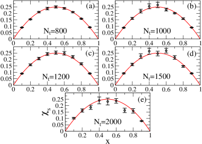
In Fig. 5 we show the fits that have been used to extract from . For all values smaller than 2000 the functional form in Eq. (27) well describes the dependence of and the values of the topological susceptibility extracted from the fits are compatible with the expected value within errors. This is not the case for , for which we obtained the quite large vale and the topological susceptibility estimate . This could be related to the fact that errors corresponding to the different determinations are for very inhomogeneous, and a fit to all the values at fixed common statistics is likely not the best choice. Of course this could become a problem in QCD, where all the slab measures would be extracted not from independent runs but from the same configurations, thus having always the same statistics for all the values. The autocorrelation of the slab measurements is shown in Fig. 6 for the case of data corresponding to and .
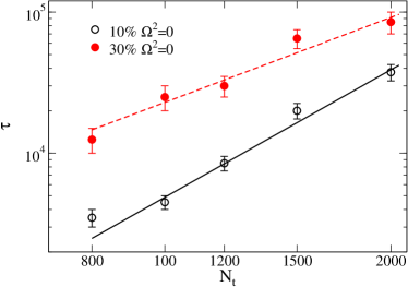
of the form to the data, while the dashed red line is a fit to the data obtained by using the functional form .
The behaviour displayed in Fig. 6 is quite easy to understand. Smaller slabs correspond to smaller autocorrelation times since they are more sensitive to the local fluctuation of the density of winding number; note however that, because of the thermal boundary conditions in time and of the fixed global topology, slices and are completely equivalent, the “worst case” being thus .
Although we do not have data precise enough to draw firm conclusions on the scaling behaviour of the autocorrelation times in the case of the slab method, it seems that autocorrelation times at fixed values are reasonably described by a power law behaviour in , with a power in the range . For the case at low temperature it is thus clear that the slab method improves a lot on the standard Metropolis algorithm.
How to extend in a systematic way this method to the case in which the probability distribution of the winding number is non-Gaussian is surely something worth further investigation. However it has to be remarked that, for theories that are not defined on a compact space, the probability distribution of the topological charge always pointwise converges to a Gaussian distribution in the thermodynamic limit555This fact is sometimes used in the literature to argue that the coefficients vanish, however this is not the case: all the cumulants grow with the volume in the thermodynamic limit and the coefficients stay constant as .. As a consequence it seems reasonable that the slab method can be safely applied whenever one is interested just in the topological susceptibility, provided the volume is large enough (i.e. ).
IV.4 Variation 4: Open boundary conditions
The fact that the winding number is an integer number is obviously related, for the model studied in this paper, to the thermal boundary conditions in time. Analogously, in 4d non-abelian gauge theories the topological charge is almost integer on the lattice due to the thermal boundary condition in the time direction and to the periodic boundary conditions in the space directions, that are typically used in order to minimize finite size effects.
Given these premises it is natural to think that the critical slowing down of the topological susceptibility could be alleviated by using different boundary conditions, that do not constraint the winding number to be integer (or almost integer). This idea was put forward in Luscher and Schaefer (2011), where the use of open boundary condition was suggested, and some interesting variations on the same theme can be found in Mages et al. (2017); Hasenbusch (2017).
The use of boundary conditions different from the thermal one in the temporal direction obviously prevent the study of the dependence of the system. However we expect the physics to be recovered independently of the specific boundary condition adopted, if the temporal extent of the lattice is large enough. In this way we move the topological slowing down problem from the ultraviolet to the infrared: the winding number is no more discrete and there can be a winding number density inflow or outflow from the boundary, however we lose translation invariance and, to avoid contaminations from surface states, we have to analyze only the part of the lattice that is far from the boundary.
The autocorrelation time of the winding number in the bulk region of the lattice is thus related to two different phenomena: the inflow/outflow from the boundary and the diffusion from the boundary to the bulk McGlynn and Mawhinney (2014). Assuming the diffusivity of the topological charge density to be well defined in the continuum limit, we thus expect the autocorrelation time of the topological susceptibility in the bulk to scale as .
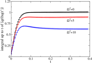
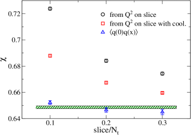
When using open boundary conditions, we want to extract information only from the part of the lattice that is far enough from the boundary as not to be influenced by its presence; as a consequence the topological susceptibility cannot be computed simply by using Eq. (15). Making use of the integral of the topological charge density restricted to a given sub-volume does not help either: we have to disentangle the true contribution of the topological susceptibility from the one of the charges that fluctuate across the boundary of the sub-volume, see Fig. 7. The best way to compute the topological susceptibility in this case is to write it as the integral of the two point function of the topological charge density (in the present case the topological charge density is simply ):
| (28) |
In this equation “” is a point in the middle of the lattice, and the lattice has to be large enough for the asymptotic value of the integral to be reached before the effects of the boundary become appreciable.
The integrand of Eq. (28) is however a very singular object for Vicari (1999); Seiler (2002): even for (at ) we have in the continuum . On the other hand, in the lattice theory, the integral in Eq. (28) reduces to a finite sum and, for this sum to converge to the integral in the continuum limit, the integrand must be well behaved as . The usual procedure that is used in cases like this is smoothing.
Many flavours of smoothing exist, like cooling Berg (1981); Iwasaki and Yoshie (1983); Itoh et al. (1984); Teper (1985); Ilgenfritz et al. (1986), smearing Albanese et al. (1987); Hasenfratz and Knechtli (2001); Morningstar and Peardon (2004) or the gradient flow Luscher (2010a, b), but the main idea is always to reduce the ultraviolet noise in a local way. While the different variants use different strategies in order to smooth the configuration (e.g., by taking local averages or by minimizing the action), in all the cases the net effect is to introduce a length and to suppress all the field fluctuations on length-scales smaller than . In order for the lattice sum to converge to the integral in Eq. (28), it is important to keep fixed in physical units as the lattice spacing is reduced.
All the smoothing algorithms have been shown to produce compatible results when their parameters are properly rescaled Bonati and D’Elia (2014); Alexandrou et al. (2015, ); Berg and Clarke (2017), so we used the computationally cheapest procedure: cooling. In order to keep fixed toward the continuum limit we rescaled the number of iterations of the cooling procedure according to the relation
| (29) |
where “round” denote the rounding to the closest integer. We then a posteriori verified that with this prescription the two point correlator smoothly converges to its continuum limit, i.e. is indeed fixed in physical unit.
For the system studied in this paper open boundary conditions in the time direction can be easily implemented by restricting the first summation in Eq. (18) to the values ; the algorithm used for the update was the same adopted for the standard Metropolis update.
The typical behaviour of the integral of two point correlation function is displayed in Fig. (8), from which we see that the integral reaches its asymptotic value around and for and respectively. This implies that a lattice extent is large enough also when using open boundary conditions.
In Fig. 9 we show the scaling of the susceptibility autocorrelation time with the inverse lattice spacing for the three cases , obtained from runs consisting of complete Metropolis sweep of the lattice. A fit using the expected behaviour is also displayed, that well describes the data for small lattice spacing values. The use of the open boundary condition thus reduces the exponential critical slowing down of periodic boundary conditions to a quadratic behaviour in the inverse of the lattice spacing.
This is obviously a great improvement, that however comes together with some difficulties. For the case of the quantum particle on a circumference the main difficulty is the impossibility of studying the thermodynamics of the model. Such a problem is obviously related to the simplicity of the model and it is not present e.g., for the case of 4d non-abelian gauge theories, in which one can use the open boundary conditions in the spatial directions. While this approach should generically work, it could present some difficulties close to a second order phase transition.
Another source of technical difficulty is related to the definition of the observables: while for the susceptibility it is relatively easy to use Eq. (28), the computation along the same lines of the higher cumulants of the winding number (needed, e.g., to extract the values of the coefficients) becomes increasingly difficult.
As observed in Sec. III the autocorrelation time is not the only figure of merit to be considered to evaluate the effectiveness of an update scheme, another important one being the CPU-time required to perform a single update. In particular one is typically interested in minimizing the statistical error attainable for unit of CPU-time at fixed external parameters (e.g. fixed lattice size). For the case of open boundary conditions a comparison with the standard Metropolis update is thus complicated by two facts:
- •
-
•
a priori different lattice sizes have to be used in the two cases to have similar finite size effects.
For the case studied in this paper these two points turned out not to be particularly important: the lattices used for the periodic boundary simulations were large enough to be used without introducing appreciable systematical errors also for the runs with open boundary conditions; moreover the variances of the two estimators adopted for the topological susceptibility were about the same. However, while the critical scaling of the autocorrelation time should be the same also for other models, these two properties cannot be expected to hold true in general.
IV.5 Variation 5: Parallel tempering
Tempering methods have been introduced in the context of the Monte Carlo simulation of spin glasses, where an exponential critical slowing down is also present, and they are based on an extended state space approach. This allows to mix together in a stochastically exact way slowly and quickly decorrelating simulations.
The tempering approach was applied for the first time to the problem of the freezing of the topological charge in Vicari (1993), where simulated tempering Marinari and Parisi (1992) was shown to be useful for the case of the 2d model, however a systematic study of its effectiveness has never been undertaken since then. More recently tempering was used to reduce the finite size effects associated with the open boundary conditions Hasenbusch (2017).
The version of tempering that we used is parallel tempering, introduced in Swendsen and Wang (1986) and later improved in Hukushima and Nemoto (1996). In this approach several simulations are performed in parallel, each one using different values of the global parameter that triggers the slowing down, in our case the lattice spacing. The global distribution of the whole system is given by the product of the distributions of the single systems. For most of the time the different simulations evolve independently of each other, but sometimes an exchange is proposed between the configurations corresponding to different lattice spacing values: of course this implies that the same value of be used for all copies, so that different lattice spacings will also correspond to different , i.e. different temperatures. The exchange of the configurations and , corresponding to lattice spacings and respectively, is accepted or rejected by a Metropolis step with acceptance probability
| (30) |
where we denoted by the value of the discretized action in Eq. (18) computed using the configuration and the value of the lattice spacing (obviously for to be real). It is easily shown that the algorithm defined in this way satisfies the detailed balance condition (see, e.g., Refs. Berg (2004); Newman and Barkema (2001)) and the advantage of the method is that the exchanges drastically reduce the autocorrelation times, since “slow” simulations are speeded up by the exchanges with the “fast” ones.
Let us assume that we are interested in simulating a lattice spacing at which the standard Metropolis algorithm decorrelates too slowly. To make use of the parallel tempering approach we have first of all to select a value at which the Metropolis algorithm is efficient, then we need to select values of the lattice spacing satisfying
| (31) |
How to select the interpolating values is a non-trivial problem, since the choice of these values strongly affects the efficiency of the algorithm.
A criterion that is commonly used to guide the choice of the intermediate values is the requirement that the probability of the exchange has to be -independent. Indeed, one can guess the autocorrelation time to be approximately given by the time required for a given configuration to reach the “quickly decorrelating” simulation, decorrelate and come back. If the acceptance probability for the various exchanges are all equal, the configuration will perform a random walk between the different copies, and the autocorrelation will be given by
| (32) |
The missing proportionality factor is determined by the acceptance ratio of the exchange step, which fixes the diffusion constant of the random walk: if adjacent lattice spacings are chosen far apart from each other, the exchange will lead to a significant increase of the global action and will be rejected most of the times.
In general it is not easy to identify intermediate values satisfying the previous requirements and several procedures exist to optimize their choice (see, e.g., Ref. Katzgraber et al. (2006); Bittner et al. (2008); Hasenbusch and Schaefer (2010)). For the case studied in this paper, however, the choice is much simpler: if we consider for the sake of the simplicity the case , the typical action of a configuration at lattice spacing is of the order of , where the typical squared displacement of the variable is of the order of . If we now consider another configuration sampled at lattice spacing and exchange them, the sum of the actions before the exchange will be of the order of , while after the exchange it will be of the order of where . The acceptance probability will thus be , with of the order of . As previously noted, for the exchange to be accepted the two lattice spacings cannot be too different from each other: has minimum at and diverges to positive values for or . This argument is obviously only approximate, since we completely neglected the role of fluctuations, however it provides an indication that the acceptance rate has to be a function of (something that we also verified numerically), meaning that in order to have equal acceptances one needs to have equal ratios between adjacent lattice spacings. The lattice spacing thus plays the same role as the temperature in a system with temperature independent specific heat, where it is known that the optimal choice is to use interpolating temperatures in geometric progression (see, e.g., Ref. Predescu et al. (2004)). As a consequence we used for the intermediate lattice spacings the values
| (33) |
To completely fix the update scheme we still have to set the value of in Eq. (33). Of course, one would like to have as small as possible in order to reduce the number of independent simulations and save computer time, however, if is too small, the ratio between adjacent lattice spacings becomes too large and the acceptance probability negligible. It is also intuitively clear that will have to be larger and larger as goes to zero with fixed, i.e. as the system gets larger and larger in lattice units, since the action is an extensive quantity. More precisely, it is a standard result (see, e.g., Ref. Hukushima and Nemoto (1996)) that, for the acceptance probability of the exchange to remain constant as , the number of copies has to scale asymptotically as follows:
| (34) |
In fact we found that, for the lattice sizes we used, the previous relation is not precise enough; for that reason, to keep the exchange acceptance probability constant as goes to zero we used the empirical formula
| (35) |
where is the constant appearing in Eq. (33) and the constant was fixed to after some preliminary tests. Using Eq. (33) we can see that the previous relation implies for the value
| (36) |
that for (with fixed) is consistent with Eq. (34).
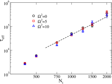
The largest lattice spacing was fixed in all the runs to , a value for which the autocorrelation time of the standard Monte Carlo update is around 10, and an exchange of the configurations corresponding to neighbouring lattice spacing values was proposed every 20 standard update sweeps. Following Eq. (36) a number of copies going from 15 to 70 was used depending on the value and, in order to keep into account the higher computational intensity of a parallel tempering run with respect to an ordinary Monte Carlo, we introduce the effective autocorrelation time defined by
| (37) |
where is the integrated autocorrelation time (in units of the elementary Metropolis update sweeps) of the topological susceptibility obtained from the run at smallest lattice spacing of the parallel tempering.
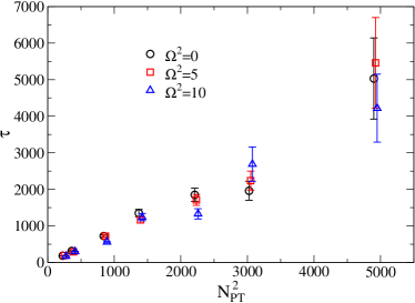
The numerical estimates of shown in Fig. (10) are obtained from simulations with a statistics of elementary updates (i.e. parallel tempering exchange steps) for each replica and again a great improvement with respect to the standard Metropolis update is clear. The behaviour of the data is roughly compatible with the scaling , slightly worse than the expected that can be obtained from Eqs. (32), (34), (37). This discrepancy is easily explained by the previous observation that our lattices are not large enough for the asymptotic expression Eq. (34) to be trusted, indeed the scaling form is instead nicely verified, as shown in Fig. 11.
IV.6 Variation 6: The very high temperature case
The numerical study of the very high temperature regime presents additional problems with respect to the low temperature case: the topological susceptibility approaches zero at high temperature, which means that the probability of observing the value of the winding number gets strongly peaked at . Indeed from Eq. (10) we can see that in the case
| (38) |
As a consequence it is very difficult to reliably estimate the values of and of the coefficients, since unfeasibly long runs are needed to compute the momenta .
For the simple case of the quantum particle moving on a circumference the high temperature problem is exacerbated by the fact that the physical volume is fixed from the beginning ( with our conventions). In 4d non-abelian gauge theories the topological susceptibility also goes to zero in the high temperature limit Gross et al. (1981); Alles et al. (1997a, b, 2000); Bonati (2015); Berkowitz et al. (2015); Bonati et al. (2016a), however the thermodynamic limit has to be performed. As a consequence, for any fixed value of (although very small) one can find a volume large enough to observe with a significant probability states with (i.e. ). While this is true in theory, in practice the size of the lattices is limited by computer resources and as a consequence also in 4d non-abelian gauge theories the study of the topological properties in the high temperature phase is particularly problematic.
The practical consequences of this problem are analogous to the ones of the freezing problem, however it has to be stressed that these two complications have completely different origins: freezing is a purely algorithmic sampling problem of the Monte Carlo, while the fact that gets strongly peaked at zero is a physical fact related to the behaviour of the topological susceptibility. It is interesting to note that none of the algorithms used so far in this paper is sufficient to study the high temperature regime, where the lattice spacing is small enough for the topological freezing to be present and .
In order to perform simulations in this regime it is first of all necessary to enhance the probability of the states, and the multicanonical approach is the best suited for this purpose. We thus add to the Euclidean action a term corresponding to the potential
| (39) |
where and are parameters of the algorithm and this potential will enter the reweight analysis procedure. The adopted values for these parameters are and (this is the optimal value for according to Eq. (38)) and simulations have been performed using the same procedure as for the simple Metropolis update. No particular optimization of the simulation parameters has been investigated, since in this section we are more interested in a proof of principle about the feasibility, rather than in an actual optimization of the runs.
As previously noted the use of the multicanonical ensemble does not solve the freezing problem, so we have to use some other algorithmic improvement on top of the multicanonical approach. The tailor method cannot be used for this purpose, since the typical configurations of the path-integral Monte-Carlo are almost straight at high temperature, also when the multicanonical term Eq. (39) is present in the Euclidean action. As a consequence it is very unlikely to find the two diametrically opposite points that are needed for the tailor update to succeed.
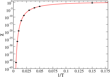
In order to avoid the freezing problem we thus adopted parallel tempering in combination with multicanonical sampling. To verify that this approach indeed allows to efficiently perform simulations in the high temperature region we used a lattice with temporal extent and lattice spacings in the range , corresponding to . We did not perform any optimization of the parameters entering in the parallel tempering, and in all the cases we just used and .
The results obtained for the topological susceptibility (with a statistics of elementary updates for each replica) using this approach are shown in Fig. 12 together with the theoretical expectation for the non-interacting case Eq. (16). The presence of a non-vanishing is in this case completely irrelevant and numerical simulations correctly reproduce the theoretical predictions over 40 orders of magnitude. Although no specific optimization of the simulation parameters has been pursued, in all cases was in the range , with a very slow increase as the lattice spacing is decreased. For the copies with the largest lattice spacings (corresponding to the lowest temperatures) we tried to also add in the simulation a tailor update step, whose effect was to reduced the autocorrelation times by an additional factor .
V Conclusions
In this study, we have considered a quantum mechanical problem which furnishes one of the simplest examples of path integral characterized by a topological classification of the configurations, and by the possible introduction of a topological term. After reviewing its main properties and some interesting exact duality relations connecting the high temperature and the low temperature regime, our main focus has been on the numerical investigation of the discretized path integral by Monte-Carlo simulations.
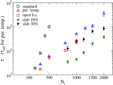
Indeed, a hard algorithmic problem which this humble model shares with nobler examples, like QCD, is the emergence of a critical slowing down of topological modes as the continuum limit is approached, leading eventually to the impossibility of properly sampling the path integral. For that reason, we have decided to explore several algorithmic improvements, some of them already proposed in the context of QCD and other field theories, in order to perform a systematic and comparative investigation of them. A summary of our results, obtained both for the free case and in the presence of a -like potential, is reported in Figs. 13 and 14.
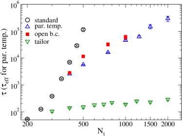
When investigating a simplified toy model in place of a more complex theory, one always faces the risk of saying something which is relevant just to the toy model and not to the original problem. We have not spent much efforts in avoiding this risk, indeed the best algorithm we have developed for the toy model is what we have named the “tailor method”, which by means of clever cuts and seams of selected pieces of configurations, achieves a direct tunneling between adjacent topological sectors which eliminates completely the problem of the so-called topological barriers. We have argued that, while the underlying symmetry concepts at the basis of the method could be exported to more complex cases, finding the proper cuts and seams is a significantly harder task in more than one space-time dimension.
However, we think that some of our findings could indeed be quite relevant also for theories like QCD. At the slab method, the method of open boundary conditions and parallel tempering provide the best results, achieving comparable efficiency in reducing the autocorrelation time of the topological susceptibility, greatly improving on the basic Metropolis scheme. From our results we obviously can not draw firm conclusions on which of these algorithms would best perform in a realistic simulation of a Yang-Mills theory or QCD, since non-universal features (like e.g. the prefactor of the scaling laws of ) could be significantly different, and the relative computational weight of the different approaches can become different from one. However parallel tempering appears to be the most flexible method of this group: the slab method is (at least in its present form) limited to the case of a Gaussian probability distribution, while the use of open boundary conditions could create some technical difficulties close to a second order phase transition and in the computation of the coefficients.
The situation is quite different when one considers the high- regime. In this case one has a new hard problem, in addition to the freezing one, namely the exponential suppression of the weight of topological sectors with , which therefore require exponentially large statistics in order to be properly sampled. Some of the methods explored at low , like the slab method and open boundary conditions, are not available in this case for the model studied here, because of the short time direction and of the absence of other space-time dimensions. The optimal strategy we have found to defeat both problems at the same time is to make use of parallel tempering in the context of a multicanonical simulation (metadynamics would work equally well). We believe that this could be a good suggestion to approach the equivalent problem one has to face in exploring the topological properties of QCD in the very high temperature regime, something which is very relevant in the context of axion phenomenology Berkowitz et al. (2015); Borsanyi et al. (2016a); Kitano and Yamada (2015); Trunin et al. (2016); Bonati et al. (2016a); Petreczky et al. (2016); Frison et al. (2016); Borsanyi et al. (2016b).
Acknowledgement We thank Francesco Sanfilippo for many useful discussions. CB wishes to thank Barbara De Palma for clarifying discussions.
References
- Aarts (2016) G. Aarts, Proceedings, 13th International Workshop on Hadron Physics: Angra dos Reis, Rio de Janeiro, Brazil, March 22-27, 2015, J. Phys. Conf. Ser. 706, 022004 (2016), arXiv:1512.05145 [hep-lat] .
- Loh et al. (1990) E. Y. J. Loh, J. E. Gubernatis, R. T. Scalettar, S. R. White, D. J. Scalapino, and R. L. Sugar, Phys. Rev. B 41, 9301 (1990).
- Troyer and Wiese (2005) M. Troyer and U.-J. Wiese, Phys. Rev. Lett. 94, 170201 (2005), arXiv:cond-mat/0408370 [cond-mat] .
- Berg (2004) B. A. Berg, Markov Chain Monte Carlo Simulations and Their Statistical Analysis (World Scientific, 2004).
- Newman and Barkema (2001) M. E. J. Newman and G. T. Barkema, Monte Carlo Methods in Statistical Physics (Clarendon Press, 2001).
- Alles et al. (1996) B. Alles, G. Boyd, M. D’Elia, A. Di Giacomo, and E. Vicari, Phys. Lett. B389, 107 (1996), arXiv:hep-lat/9607049 [hep-lat] .
- Schaefer et al. (2011) S. Schaefer, R. Sommer, and F. Virotta (ALPHA), Nucl. Phys. B 845, 93 (2011), arXiv:1009.5228 [hep-lat] .
- Bonati et al. (2016a) C. Bonati, M. D’Elia, M. Mariti, G. Martinelli, M. Mesiti, F. Negro, F. Sanfilippo, and G. Villadoro, JHEP 03, 155 (2016a), arXiv:1512.06746 [hep-lat] .
- Campostrini et al. (1992) M. Campostrini, P. Rossi, and E. Vicari, Phys. Rev. D46, 2647 (1992).
- Del Debbio et al. (2002) L. Del Debbio, H. Panagopoulos, and E. Vicari, JHEP 08, 044 (2002), arXiv:hep-th/0204125 [hep-th] .
- Del Debbio et al. (2004) L. Del Debbio, G. M. Manca, and E. Vicari, Phys. Lett. B594, 315 (2004), arXiv:hep-lat/0403001 [hep-lat] .
- (12) J. Flynn, A. Juttner, A. Lawson, and F. Sanfilippo, “Precision study of critical slowing down in lattice simulations of the model,” 2015, arXiv:1504.06292 [hep-lat] .
- Berkowitz et al. (2015) E. Berkowitz, M. I. Buchoff, and E. Rinaldi, Phys. Rev. D92, 034507 (2015), arXiv:1505.07455 [hep-ph] .
- Borsanyi et al. (2016a) S. Borsanyi, M. Dierigl, Z. Fodor, S. D. Katz, S. W. Mages, D. Nogradi, J. Redondo, A. Ringwald, and K. K. Szabo, Phys. Lett. B752, 175 (2016a), arXiv:1508.06917 [hep-lat] .
- Kitano and Yamada (2015) R. Kitano and N. Yamada, JHEP 10, 136 (2015), arXiv:1506.00370 [hep-ph] .
- Trunin et al. (2016) A. Trunin, F. Burger, E.-M. Ilgenfritz, M. P. Lombardo, and M. Müller-Preussker, Proceedings, 15th International Conference on Strangeness in Quark Matter (SQM 2015): Dubna, Moscow region, Russia, July 6-11, 2015, J. Phys. Conf. Ser. 668, 012123 (2016), arXiv:1510.02265 [hep-lat] .
- Petreczky et al. (2016) P. Petreczky, H.-P. Schadler, and S. Sharma, Phys. Lett. B762, 498 (2016), arXiv:1606.03145 [hep-lat] .
- Frison et al. (2016) J. Frison, R. Kitano, H. Matsufuru, S. Mori, and N. Yamada, JHEP 09, 021 (2016), arXiv:1606.07175 [hep-lat] .
- Borsanyi et al. (2016b) S. Borsanyi et al., Nature 539, 69 (2016b), arXiv:1606.07494 [hep-lat] .
- Jackiw (1980) R. Jackiw, Rev. Mod. Phys. 52, 661 (1980).
- Treiman et al. (1985) S. B. Treiman, R. Jackiw, B. Zumino, and E. Witten, Current algebra and anomalies (Princeton University Press, 1985).
- Smilga (2001) A. Smilga, Lectures on Quantum Chrmodynamics (World Scientific, 2001).
- Strocchi (2013) F. Strocchi, An Introduction to Non-Perturbative Foundations of Quantum Field Theory (Oxford University Press, 2013).
- Krauth (2006) W. Krauth, Statistical Mechanics: Algorithms and Computations (Oxford University Press, 2006).
- Coleman (1988) S. Coleman, Aspects of symmetry (Cambridge University Press, 1988).
- Vafa and Witten (1984) C. Vafa and E. Witten, Phys. Rev. Lett. 53, 535 (1984).
- Peccei and Quinn (1977a) R. D. Peccei and H. R. Quinn, Phys. Rev. Lett. 38, 1440 (1977a).
- Peccei and Quinn (1977b) R. D. Peccei and H. R. Quinn, Phys. Rev. D 16, 1791 (1977b).
- Bellman (2013) R. Bellman, A Brief Introduction to Theta Functions (Dover Publications, 2013).
- Whittaker and Watson (1996) E. T. Whittaker and G. N. Watson, A course of modern analysis (Cambridge University Press, 1996).
- Witten (1980) E. Witten, Annals Phys. 128, 363 (1980).
- Witten (1998) E. Witten, Phys. Rev. Lett. 81, 2862 (1998), arXiv:hep-th/9807109 [hep-th] .
- Gaiotto et al. (2017) D. Gaiotto, A. Kapustin, Z. Komargodski, and N. Seiberg, JHEP 05, 091 (2017), arXiv:1703.00501 [hep-th] .
- Di Vecchia and Veneziano (1980) P. Di Vecchia and G. Veneziano, Nucl. Phys. B 171, 253 (1980).
- (35) D. Gaiotto, Z. Komargodski, and N. Seiberg, “Time-Reversal Breaking in QCD4, Walls, and Dualities in 2+1 Dimensions,” 2017, arXiv:1708.06806 [hep-th] .
- Di Vecchia et al. (2017) P. Di Vecchia, G. Rossi, G. Veneziano, and S. Yankielowicz, JHEP 12, 104 (2017), arXiv:1709.00731 [hep-th] .
- Gross et al. (1981) D. J. Gross, R. D. Pisarski, and L. G. Yaffe, Rev. Mod. Phys. 53, 43 (1981).
- Vicari and Panagopoulos (2009) E. Vicari and H. Panagopoulos, Phys. Rept. 470, 93 (2009), arXiv:0803.1593 [hep-th] .
- Azcoiti et al. (2002) V. Azcoiti, G. Di Carlo, A. Galante, and V. Laliena, Phys. Rev. Lett. 89, 141601 (2002), arXiv:hep-lat/0203017 [hep-lat] .
- Alles and Papa (2008) B. Alles and A. Papa, Phys. Rev. D77, 056008 (2008), arXiv:0711.1496 [cond-mat.stat-mech] .
- Alles et al. (2014) B. Alles, M. Giordano, and A. Papa, Phys. Rev. B90, 184421 (2014), arXiv:1409.1704 [hep-lat] .
- Panagopoulos and Vicari (2011) H. Panagopoulos and E. Vicari, JHEP 11, 119 (2011), arXiv:1109.6815 [hep-lat] .
- D’Elia and Negro (2012) M. D’Elia and F. Negro, Phys. Rev. Lett. 109, 072001 (2012), arXiv:1205.0538 [hep-lat] .
- D’Elia and Negro (2013) M. D’Elia and F. Negro, Phys. Rev. D88, 034503 (2013), arXiv:1306.2919 [hep-lat] .
- Bonati et al. (2016b) C. Bonati, M. D’Elia, and A. Scapellato, Phys. Rev. D93, 025028 (2016b), arXiv:1512.01544 [hep-lat] .
- Bonati et al. (2016c) C. Bonati, M. D’Elia, P. Rossi, and E. Vicari, Phys. Rev. D94, 085017 (2016c), arXiv:1607.06360 [hep-lat] .
- Madras and Sokal (1988) N. Madras and A. D. Sokal, J. Stat. Phys. 50, 109 (1988).
- Wolff (2004) U. Wolff (ALPHA), Comput. Phys. Commun. 156, 143 (2004), [Erratum: Comput. Phys. Commun. 176, 383 (2007)], arXiv:hep-lat/0306017 [hep-lat] .
- (49) B. De Palma, M. Erba, L. Mantovani, and N. Mosco, “A Python program for the implementation of the -method for Monte Carlo simulations,” 2017, arXiv:1703.02766 [hep-lat] .
- Muller-Krumbhaar and Binder (1973) H. Muller-Krumbhaar and K. Binder, J. Stat. Phys. 8, 1 (1973).
- Metropolis et al. (1953) N. Metropolis, A. W. Rosenbluth, M. N. Rosenbluth, A. H. Teller, and E. Teller, The J. of Chem. Phys. 21, 1087 (1953).
- Creutz and Freedman (1981) M. Creutz and B. Freedman, Annals of Phys. 132, 427 (1981).
- Berg and Neuhaus (1992) B. A. Berg and T. Neuhaus, Phys. Rev. Lett. 68, 9 (1992), arXiv:hep-lat/9202004 [hep-lat] .
- Laio and Parrinello (2002) A. Laio and M. Parrinello, Proceedings of the National Academy of Sciences 99, 12562 (2002), arXiv:0208352 [cond-mat] .
- Laio and Gervasio (2008) A. Laio and F. L. Gervasio, Rep. Prog. Phys. 71, 126601 (2008).
- Laio et al. (2016) A. Laio, G. Martinelli, and F. Sanfilippo, JHEP 07, 089 (2016), arXiv:1508.07270 [hep-lat] .
- Wang and Landau (2001) F. Wang and D. P. Landau, Phys. Rev. Lett. 86, 2050 (2001), arXiv:0011174 [cond-mat] .
- Langfeld et al. (2012) K. Langfeld, B. Lucini, and A. Rago, Phys. Rev. Lett. 109, 111601 (2012), arXiv:1204.3243 [hep-lat] .
- Cossu et al. (2017) G. Cossu, B. Lucini, R. Pellegrini, and A. Rago, in 35th International Symposium on Lattice Field Theory (Lattice 2017) Granada, Spain, June 18-24, 2017 (2017) arXiv:1710.06250 [hep-lat] .
- Wolff (1989) U. Wolff, Phys. Rev. Lett. 62, 361 (1989).
- Brower and Tamayo (1989) R. C. Brower and P. Tamayo, Phys. Rev. Lett. 62, 1087 (1989).
- Evertz et al. (1991) H. G. Evertz, M. Hasenbusch, M. Marcu, K. Pinn, and S. Solomon, Phys. Lett. 254B, 185 (1991).
- Ceperley and Pollock (1986) D. M. Ceperley and E. L. Pollock, Phys. Rev. Lett. 56, 351 (1986).
- Goodman and Sokal (1986) J. Goodman and A. D. Sokal, Phys. Rev. Lett. 56, 1015 (1986).
- Ceperley (1995) D. M. Ceperley, Rev. Mod. Phys. 67, 279 (1995).
- Goodman and Sokal (1989) J. Goodman and A. D. Sokal, Phys. Rev. D 40, 2035 (1989).
- Shuryak and Verbaarschot (1995) E. V. Shuryak and J. J. M. Verbaarschot, Phys. Rev. D 52, 295 (1995), arXiv:hep-lat/9409020 [hep-lat] .
- de Forcrand et al. (1999) P. de Forcrand, M. Garcia Perez, J. E. Hetrick, E. Laermann, J. F. Lagae, and I. O. Stamatescu, in Lattice Field Theory. Proceedings: 16th International Symposium, Lattice ’98, Boulder, USA, Jul 13-18, 1998, Vol. 73 (1999) pp. 578–580, [,578(1998)], arXiv:hep-lat/9810033 [hep-lat] .
- Bietenholz et al. (2015) W. Bietenholz, P. de Forcrand, and U. Gerber, JHEP 12, 070 (2015), arXiv:1509.06433 [hep-lat] .
- Bietenholz et al. (2016) W. Bietenholz, K. Cichy, P. de Forcrand, A. Dromard, and U. Gerber, in Proceedings, 34th International Symposium on Lattice Field Theory (Lattice 2016): Southampton, UK, July 24-30, 2016, Vol. LATTICE2016 (2016) p. 321, arXiv:1610.00685 [hep-lat] .
- Bonati et al. (2013) C. Bonati, M. D’Elia, H. Panagopoulos, and E. Vicari, Phys. Rev. Lett. 110, 252003 (2013), arXiv:1301.7640 [hep-lat] .
- Bonati (2015) C. Bonati, JHEP 03, 006 (2015), arXiv:1501.01172 [hep-lat] .
- Luscher and Schaefer (2011) M. Luscher and S. Schaefer, JHEP 07, 036 (2011), arXiv:1105.4749 [hep-lat] .
- Mages et al. (2017) S. Mages, B. C. Toth, S. Borsanyi, Z. Fodor, S. D. Katz, and K. K. Szabo, Phys. Rev. D 95, 094512 (2017), arXiv:1512.06804 [hep-lat] .
- Hasenbusch (2017) M. Hasenbusch, Phys. Rev. D96, 054504 (2017), arXiv:1706.04443 [hep-lat] .
- McGlynn and Mawhinney (2014) G. McGlynn and R. D. Mawhinney, Phys. Rev. D90, 074502 (2014), arXiv:1406.4551 [hep-lat] .
- Vicari (1999) E. Vicari, Nucl. Phys. B554, 301 (1999), arXiv:hep-lat/9901008 [hep-lat] .
- Seiler (2002) E. Seiler, Phys. Lett. B525, 355 (2002), arXiv:hep-th/0111125 [hep-th] .
- Berg (1981) B. Berg, Phys. Lett. 104B, 475 (1981).
- Iwasaki and Yoshie (1983) Y. Iwasaki and T. Yoshie, Phys. Lett. 131B, 159 (1983).
- Itoh et al. (1984) S. Itoh, Y. Iwasaki, and T. Yoshie, Phys. Lett. 147B, 141 (1984).
- Teper (1985) M. Teper, Phys. Lett. 162B, 357 (1985).
- Ilgenfritz et al. (1986) E.-M. Ilgenfritz, M. L. Laursen, G. Schierholz, M. Muller-Preussker, and H. Schiller, Proceedings, 23RD International Conference on High Energy Physics, JULY 16-23, 1986, Berkeley, CA, Nucl. Phys. B268, 693 (1986).
- Albanese et al. (1987) M. Albanese et al. (APE), Phys. Lett. B192, 163 (1987).
- Hasenfratz and Knechtli (2001) A. Hasenfratz and F. Knechtli, Phys. Rev. D64, 034504 (2001), arXiv:hep-lat/0103029 [hep-lat] .
- Morningstar and Peardon (2004) C. Morningstar and M. J. Peardon, Phys. Rev. D69, 054501 (2004), arXiv:hep-lat/0311018 [hep-lat] .
- Luscher (2010a) M. Luscher, Commun. Math. Phys. 293, 899 (2010a), arXiv:0907.5491 [hep-lat] .
- Luscher (2010b) M. Luscher, JHEP 08, 071 (2010b), [Erratum: JHEP03,092(2014)], arXiv:1006.4518 [hep-lat] .
- Bonati and D’Elia (2014) C. Bonati and M. D’Elia, Phys. Rev. D89, 105005 (2014), arXiv:1401.2441 [hep-lat] .
- Alexandrou et al. (2015) C. Alexandrou, A. Athenodorou, and K. Jansen, Phys. Rev. D92, 125014 (2015), arXiv:1509.04259 [hep-lat] .
- (91) C. Alexandrou, A. Athenodorou, K. Cichy, A. Dromard, E. Garcia-Ramos, K. Jansen, U. Wenger, and F. Zimmermann, “Comparison of topological charge definitions in Lattice QCD,” 2017, arXiv:1708.00696 [hep-lat] .
- Berg and Clarke (2017) B. A. Berg and D. A. Clarke, Phys. Rev. D95, 094508 (2017), arXiv:1612.07347 [hep-lat] .
- Vicari (1993) E. Vicari, Phys. Lett. B309, 139 (1993), arXiv:hep-lat/9209025 [hep-lat] .
- Marinari and Parisi (1992) E. Marinari and G. Parisi, Europhys. Lett. 19, 451 (1992), arXiv:hep-lat/9205018 [hep-lat] .
- Swendsen and Wang (1986) R. H. Swendsen and J.-S. Wang, Phys. Rev. Lett. 57, 2607 (1986).
- Hukushima and Nemoto (1996) K. Hukushima and K. Nemoto, J. Phys. Soc. Jan. 65, 1604 (1996), arXiv:9512035 [cond-mat] .
- Katzgraber et al. (2006) H. G. Katzgraber, S. Trebst, D. A. Huse, and T. Matthias, J. Stat. Mech 2006, P03018 (2006), arXiv:0602085 [cond-mat] .
- Bittner et al. (2008) E. Bittner, A. Nussbaumer, and J. Janke, Phys. Rev. Lett 101, 130603 (2008), arXiv:0809.0571 [cond-mat] .
- Hasenbusch and Schaefer (2010) M. Hasenbusch and S. Schaefer, Phys. Rev. E 82, 046707 (2010), arXiv:1006.4247 [cond-mat.stat-mech] .
- Predescu et al. (2004) C. Predescu, M. Predescu, and C. V. Ciobanu, J. Chem. Phys. 120, 4119 (2004).
- Alles et al. (1997a) B. Alles, M. D’Elia, and A. Di Giacomo, Nucl. Phys. B494, 281 (1997a), [Erratum: Nucl. Phys.B679,397(2004)], arXiv:hep-lat/9605013 [hep-lat] .
- Alles et al. (1997b) B. Alles, M. D’Elia, and A. Di Giacomo, Phys. Lett. B412, 119 (1997b), arXiv:hep-lat/9706016 [hep-lat] .
- Alles et al. (2000) B. Alles, M. D’Elia, and A. Di Giacomo, Phys. Lett. B483, 139 (2000), arXiv:hep-lat/0004020 [hep-lat] .