DIeSEL: DIstributed SElf-Localization of a network of underwater vehicles

Abstract

How can teams of artificial agents localize and position themselves in GPS-denied environments? How can each agent determine its position from pairwise ranges, own velocity, and limited interaction with neighbors? This paper addresses this problem from an optimization point of view: we directly optimize the nonconvex maximum-likelihood estimator in the presence of range measurements contaminated with Gaussian noise, and we obtain a provably convergent, accurate and distributed positioning algorithm that outperforms the extended Kalman filter, a standard centralized solution for this problem.

I Introduction

The deployment of networked systems of agents that can interact with the physical world and carry out complex tasks in heterogeneous environments is currently a major driver for research and technological development. This trend is also seen in contemporary ocean applications and it propelled research projects on multi-vehicle systems like WiMUST (Al-Khatib et al. [1]). Our work concerns localization of (underwater) vehicle formations, a key subsystem needed in the absence of GPS to properly georeference any acquired data and also used in cooperative control algorithms.

Related work

The signal processing and control communities studied the network localization problem in many variants, like static or dynamic network localization, centralized or distributed computations, maximum-likelihood methods, approximation algorithms, or outlier robust methods.

The control community’s mainstream approach to localization relies on the robust and strong properties of the Kalman filter to dynamically compensate noise and bias. Recent approaches can be found in Pinheiro et al. [2] and Rad et al. [3]. In the first very recent paper, position and velocity are estimated from ranges, accelerometer readings and gyroscope measurements with an Extended Kalman filter. The authors of the second paper linearize the range-only dynamic network localization problem, solving it with a linear Kalman filter.

Our optimization-based approach is mainly inspired by the literature on sensor network localization, or static cooperative localization, using pairwise range measurements. Shang et al. [4] follow a multidimensional scaling approach, but multidimensional scaling works well only in networks with high connectivity — a property not encountered in practice in large-scale geometric networks. Biswas et al. [5] and Oğuz-Ekim et al. [6] proposed semi-definite and second order cone relaxations of the maximum likelihood estimator. Although more precise, these convexified problems get intractable even for a small number of nodes. The methods in Calafiore et al. [7] and Soares et al. [8] increase the precision of an initial good guess, but are prone to local minima if wrongly initialized. To disambiguate the spatial configuration, classic static range-based localization requires a minimum of three non-collinear anchors (i.e., reference points with known position) for a planar network and four anchors for a volumetric one. In practice, the number of anchors might be larger to attain the desired positioning accuracy. Lately, signal processing researchers produced solutions for dynamic network localization; Schlupkothen et al. [9] and Soares et al. [10] incorporated velocity information from past position estimates to bias the solution of a static relaxation of the localization problem via a regularization term.

In our work we exploit the fact that underwater vehicles are sophisticated nodes that often provide additional measurements besides ranges, such as depth (from pressure sensors) and relative velocity (from DVL). We leverage this side information to reduce the required number of anchors, which might be cumbersome or costly to deploy in underwater applications — for example, when anchors are GPS-enabled surface vehicles every reduction affords substantial savings in terms of logistics and budget.

Our approach

We adopt a data model for cooperative localization of underwater vehicle formations consisting of a modest number, or even a single anchor and measurements for ranges, depths, and vehicle velocities relative to the water, whenever these quantities are available. We formulate the problem as a maximum-likelihood estimation problem assuming noise on the range measurements. We derive a distributed algorithm to provably attain a stationary point of the nonconvex maximum-likelihood estimator.

II Problem formulation

We denote the measurement and communication graph connecting vehicles as $\mathcal{G}=(\mathcal{V},\mathcal{E})$, where the node set $\mathcal{V}=\{1,2,\cdots,n\}$ represents the ensemble of vehicles with unknown positions. Edge $i\sim j\in\mathcal{E}$ means that there is a range measurement and a communication link between nodes $i$ and $j$. The set of vehicles with known positions, also called anchors, is denoted $\mathcal{A}=\{1,\cdots,m\}$ and we assume $m$ small (as low as $m=1$). For each $i\in\mathcal{V}$, we let $\mathcal{A}_{i}\in\mathcal{A}$ be the subset of anchors (if any) relative to which node $i$ also possesses a noisy range measurement. To simplify notation, and without loss of generality, we omit the explicit dependency in time of graph $\mathcal{G}$.

Let $\mathbb{R}^{d}$ be the space of interest, where $d=2$ whenever the vehicles move in a planar configuration or when we have access to the depth of all vehicles, and $d=3$ otherwise, $p_{i}\in\mathbb{R}^{d}$ is the position of vehicle $i$ at some discrete time instant $t-T_{0}$, with $T_{0}$ as a convenient time window, $v^{I}_{i}(t)=v^{R}_{i}(t)+v_{f}$ is the inertial velocity at the discrete time instant $t$, where $v^{R}_{i}(t)$ is vehicle’s $i$ known velocity relative to the fluid, and $v_{f}\in\mathbb{R}^{d}$ is the unknown fluid velocity (current), assumed constant in space and time. We define $v_{i}(t)=\sum_{\tau=t-T_{0}}^{t}v_{i}^{R}(\tau)$. Thus, the position of node $i$ at a time $t$ is $x_{i}(t)=p_{i}+\sum_{\tau=t-T_{0}}^{t}v_{i}^{I}(\tau)\Delta T$, where $\Delta T$ is the sampling interval. Let $d_{ij}(t)$ be the noisy range measurement between vehicles $i$ and $j$ at time $t$, known by both $i$ and $j$. Without loss of generality, we assume $d_{ij}(t)=d_{ji}(t)$. Anchor positions are denoted by $a_{k}(t)\in\mathbb{R}^{d}$. Similarly, $r_{ik}(t)$ is the noisy range measurement between node $i$ and anchor $k$. Define $x(t)=\{x_{i}(t):i\in\mathcal{V}\}$ as the concatenation of all unknown vehicle positions at time $t$.

The distributed network localization problem addressed in this work consists in estimating the set of vehicles’ positions $x(t)$, from the available measurements $\{d_{ij}(t):i\sim j\}\cup\{r_{ik}(t):i\in\mathcal{V},k\in\mathcal{A}_{i}\}$, through cooperative message passing between neighboring sensors in the communication graph $\mathcal{G}$. Under the assumption of zero-mean, independent and identically-distributed, additive Gaussian measurement noise, the maximum likelihood estimator for the sensor positions at time $t$ is the solution of the optimization problem

$$\operatornamewithlimits{minimize}f_{T_{0},t}(x(t)),$$ (1)

where the cost is defined as

$$\begin{split}f_{T_{0},t}(x(t))=&\sum_{\tau=t-T_{0}}^{t}\left(\sum_{i\sim j}\frac{1}{2}(\|x_{i}(\tau)-x_{j}(\tau)\|-d_{ij}(\tau))^{2}+\right.\\ &\left.\sum_{i}\sum_{k\in\mathcal{A}_{i}}\frac{1}{2}(\|x_{i}(\tau)-a_{k}(\tau)\|-r_{ik}(\tau))^{2}\right).\end{split}$$ (2)

III Underwater localization

Define $x_{i}=\{x_{i}(\tau)\}$ and introduce two sets of auxiliary variables $y_{ij}=\{y_{ij}(\tau)\}$ and $w_{ik}=\{w_{ik}(\tau)\}$. Adopting the approach of [8] we can reformulate problem (1) as

$$\begin{split}\operatornamewithlimits{minimize}_{\{x_{i}\},\{y_{ij}\},\{w_{ik}\}}&\sum_{i\sim j}\sum_{\tau=t-T_{0}}^{t}\frac{1}{2}\|x_{i}(\tau)-x_{j}(\tau)-y_{ij}(\tau)\|^{2}+\\ &\sum_{i}\sum_{k\in\mathcal{A}_{i}}\sum_{\tau=t-T_{0}}^{t}\frac{1}{2}\|x_{i}(\tau)-a_{k}(\tau)-w_{ik}(\tau)\|^{2}\\ \operatornamewithlimits{\text{subject to}}&\|y_{ij}(\tau)\|=d_{ij}(\tau),\;\forall i\sim j\\ &\|w_{ik}(\tau)\|=r_{ik}(\tau),\;\forall i\in\mathcal{V},k\in\mathcal{A}_{i}.\end{split}$$ (3)

We now notice that the subtraction $x_{i}(\tau)-x_{j}(\tau)$ cancels out the fluid velocity, obtaining, for both node-node and node-anchor pairs,

$$\begin{split}x_{i}(\tau)-x_{j}(\tau)&=p_{i}-p_{j}+(v_{i}(\tau)-v_{j}(\tau))\Delta T\\ x_{i}(\tau)-a_{k}(\tau)&=p_{i}-q_{k}+(v_{i}(\tau)-u_{k}(\tau))\Delta T.\end{split}$$

where the anchor decomposed as $a_{k}(\tau)=q_{k}+u_{k}(\tau)\Delta T$ mirrors the aforementioned decomposition for nodes. Define the concatenation $z=(\{p_{i}\},\{y_{ij}\},\{w_{ik}\})$, where $y_{ij}=\{y_{ij}(\tau)\}$ and $w_{ik}=\{w_{ik}(\tau)\}$ stack $y_{ij}(\tau)$ and $w_{ik}(\tau)$ for all time instants from $\tau=t-T_{0}$ to $\tau=t$, and the constraint set

$$\mathcal{Z}=\{z:\|y_{ij}\|=d_{ij}\forall i\sim j,\|w_{ik}\|=r_{ik}\forall i\in\mathcal{V},k\in\mathcal{A}_{i}\}.$$ (4)

The terms in $\tau$ in the cost of problem (3) can be stacked, thus obtaining the problem

$$\begin{array}[]{rl}\operatornamewithlimits{minimize}&\frac{1}{2}\|DAp+\Delta v-y\|^{2}+\frac{1}{2}\|Ep-\alpha-w\|^{2},\\ \operatornamewithlimits{\text{subject to}}&(p,y,w)\in\mathcal{Z}\end{array}$$ (5)

where we denote matrix $A$ as the Kronecker product of the arc-node incidence matrix $C$ of the measurement graph $\mathcal{G}$ with the identity matrix $I_{d}$, matrix $D$ is a tall concatenation of identity matrices and matrix $E$ is a selector with zeros and ones. The constant $\Delta v$ is defined as

$$\Delta v=\{(v_{i}(\tau)-v_{j}(\tau))\Delta T,\text{ for all }\;i\sim j,t-T_{0}\leq\tau\leq t\},$$

and the anchor term’s non-optimized data term is

$$\begin{split}\alpha=&\{q_{k}-(v_{i}(\tau)-u_{k}(\tau))\Delta T,\\ &\text{ for all }\;i\in\mathcal{V},k\in\mathcal{A}_{i},t-T_{0}\geq\tau\geq t\}.\end{split}$$

With this notation, Problem (5) is equivalent to

$$\begin{array}[]{rl}\operatornamewithlimits{minimize}&\frac{1}{2}\left\|\begin{bmatrix}DA&-I&0\end{bmatrix}\begin{bmatrix}p\\ y\\ w\end{bmatrix}+\Delta v\right\|^{2}+\\ &\frac{1}{2}\left\|\begin{bmatrix}E&0&-I\end{bmatrix}\begin{bmatrix}p\\ y\\ w\end{bmatrix}-\alpha\right\|^{2}\\ \operatornamewithlimits{\text{subject to}}&(p,y,z)\in\mathcal{Z}.\end{array}$$

The cost can be further simplified as

$$\begin{array}[]{rl}\operatornamewithlimits{minimize}&F_{T_{0},t}(z)=\frac{1}{2}z^{T}Mz-b^{T}z\\ \operatornamewithlimits{\text{subject to}}&z\in\mathcal{Z}\end{array}$$ (6)

where matrix $M$ is

$$M=\begin{bmatrix}A^{T}D^{T}DA+E^{T}E&-A^{T}D^{T}&-E^{T}\\ -DA&I&0\\ -E&0&I\end{bmatrix},$$

and vector $b$ is

$$b=\begin{bmatrix}E^{T}\\ 0\\ -I\end{bmatrix}\alpha-\begin{bmatrix}A^{T}D^{T}\\ -I\\ 0\end{bmatrix}\Delta v.$$

The cost in problem (6) is quadratic, but as its minimization is constrained to a nonconvex set it retains the hardness of the original, equivalent, problem (1). Also, off-diagonal terms in matrix $M$ couple variables for the different vehicles, which impedes a distributed solution. In the next section we will approach these issues to achieve a distributed positioning algorithm with provable convergence.

IV Distributed underwater localization

Problem (6) is a quadratic cost constrained to a nonconvex set, which is a very hard optimization problem, in general. Further, the off-diagonal terms couple the vehicles’ variables, thus preventing a distributed solution. Nevertheless, we are now, at each time step, in the conditions of the algorithm presented in [8]. From here on we adapt the results of this reference to the current problem.

We now call the reader’s attention for the fact that every quadratic function has a Lipschitz continuous gradient, meaning that we can majorize our correlated quadratic with a diagonal scale term, the Lipschitz constant $L$ associated with the function’s gradient

$$\begin{split}F_{T_{0},t}(z)\leq&F_{T_{0},t}(z(\kappa))+\langle\nabla F_{T_{0},t}(z(\kappa)),z-z(\kappa)\rangle+\\ &\frac{L}{2}\|z-z(\kappa)\|^{2},\end{split}$$

valid for any points $z,$ and $z(k)$. We iteratively majorize the quadratic coupled cost by this quadratic diagonal upper bound of the cost, and then minimize the majorizer, under the framework of a Majorization-Minimization algorithm. Here the algorithm steps are denoted by $\kappa$, to avoid confusion with the discrete time running on $t$. Minimization of the majorizer can be written as

$$\begin{split}z(\kappa+1)=\operatornamewithlimits{argmin}_{z\in\mathcal{Z}}&F_{T_{0},t}(z(\kappa))+\langle\nabla F_{T_{0},t}(z(\kappa)),z-z(\kappa)\rangle+\\ &+\frac{L}{2}\|z-z(\kappa)\|^{2}.\end{split}$$ (7)

The solution to Problem (7) is the well-known projected gradient iteration

$$z(\kappa+1)=\mathrm{P}_{\mathcal{Z}}\left(z(\kappa)-\frac{1}{L}\nabla F_{T_{0},t}(z(\kappa))\right),$$ (8)

where $\mathrm{P}_{\mathcal{Z}}(z)$ is the projection of point $z$ onto set $\mathcal{Z}$. The gradient $\nabla F_{T_{0},t}(z)$ is simply

$$\nabla F_{T_{0},t}(z)=Mz-b,$$

and a Lipschitz constant $L$ associated with the gradient $\nabla F_{T_{0},t}(z)$ to compute the gradient step in (8) turns out to be $L=T_{0}(2\delta_{\mathrm{max}}+\max_{i}|\mathcal{A}_{i}|)+2$, where $\delta_{\mathrm{max}}$ is the maximum node degree in the network.

Algorithm 1 DIeSEL: Distributed Self-Localization

0:    $L;$ $z=(p,y,w);$$\beta_{i}=\frac{L-T_{0}(\delta_{i}-|\mathcal{A}_{i}|)}{L};$ $\{d_{ij}(t):i\sim j\in\mathcal{E}\};$ // acquired as time $t$ evolves$\{r_{ik}(t):i\in\mathcal{V},k\in\mathcal{A}\};$ // acquired as time $t$ evolves

0:  $\hat{z}=\{(p_{i},y_{ij},w_{ik})\}$

1:  for all $t\in\{T_{0},...\}$ do

2:     $\kappa=1$$\Delta v_{ij}=\{(v_{i}(\tau)-v_{j}(\tau))\Delta T,\text{ for all }t-T_{0}\leq\tau\leq t\}$ $\Delta u_{ik}=\{(v_{i}(\tau)-u_{k}(\tau))\Delta T,\text{ for all }t-T_{0}\leq\tau\leq t\}$

3:     while some stopping criterion is not met, each node $i$ do

4:        broadcast $p_{i}$ to all neighbors

5:        

$$\begin{split}p_{i}^{+}=&\beta_{i}p_{i}+\\ &\sum_{j\in\mathcal{N}_{i}}\sum_{\tau=t-T_{0}}^{t}\left(p_{j}+C_{(i\sim j,i)}y_{ij}(\tau)+\Delta v_{ij}(\tau)\right)+\\ &\sum_{k\in|\mathcal{A}_{i}|}\sum_{\tau=t-T_{0}}^{t}\left(a_{k}+w_{ik}(\tau)+\Delta u_{ik}(\tau)\right)\end{split}$$

6:        for all  $j$, $i\sim j$, and $\tau\in[t-T_{0};t]$ do

7:           

$$\begin{split}y_{ij}^{+}(\tau)=&\mathrm{P}_{\mathcal{Y}_{ij}(\tau)}\Big{(}\frac{L-1}{L}y_{ij}(\tau)+\\ &\frac{1}{L}C_{(i\sim j,i)}(p_{i}-p_{j}-\Delta v_{ij}(\tau))\Big{)}\end{split}$$

8:        end for

9:        for all  $k\in\mathcal{A}_{i}$, and $\tau\in[t-T_{0};t]$ do

10:           

$$w_{ik}^{+}(\tau)=\mathrm{P}_{\mathcal{W}_{ik}(\tau)}\left(\frac{L-1}{L}w_{ik}(\tau)+\frac{1}{L}(p_{i}-a_{k}-\Delta u_{ik}(\tau))\right)$$

11:        end for

12:        update $\kappa=\kappa+1;$ $(p_{i},y_{ij},w_{ik})=(p_{i}^{+},y_{ij}^{+},w_{ik}^{+})$

13:     end while

14:  end for

Algorithm 1 summarizes the distributed operation of our proposed method. Results presented in [11] guarantee convergence of the algorithm to a stationary point.

V Simulation results

To assess the quality of the algorithm we compared it with a centralized Extended Kalman Filter (EKF) and with a static optimization-based distributed algorithm, which only uses noisy ranges and anchor positions. The EKF parameters were tuned for every trajectory. For DIeSEL, we assigned the same time window $T_{0}=5$ for all trajectories, unless otherwise noted. The static range-only method has no parameters to tune.

We ran numerical simulations with a four-vehicle team where the center two vehicles are GPS-enabled (i.e., anchors). The other two navigate only with noisy range measurements and inertial velocities.

(a) Lap trajectory, with four vehicles (distances in meters).

(b) Descending helix.

(c) The lawn mower trajectory.

Figure 1: Trajectories for experimental evaluation. Each starting position is marked with a plus sign.

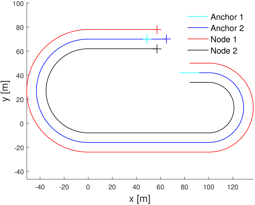
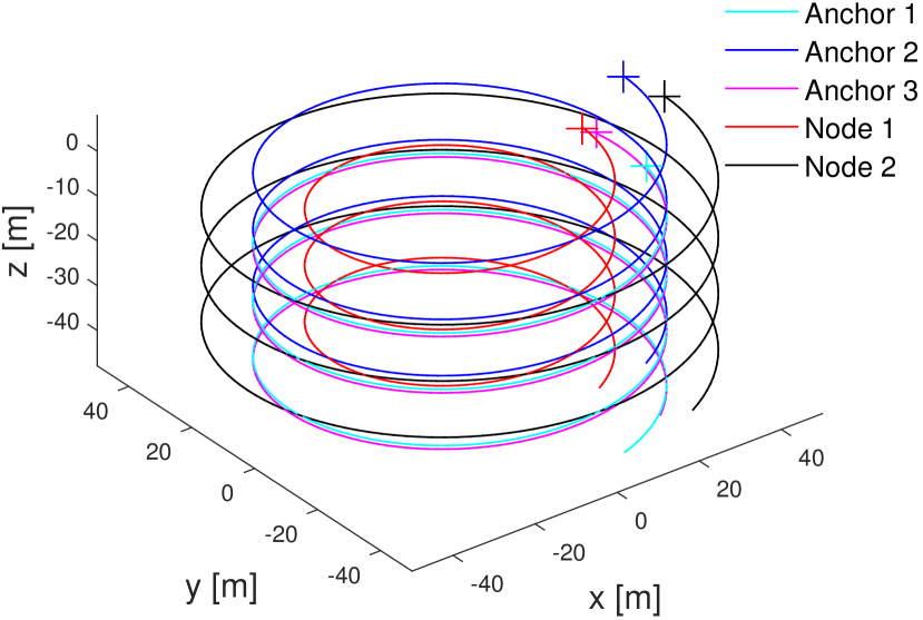
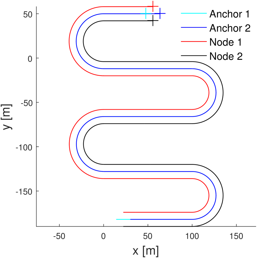
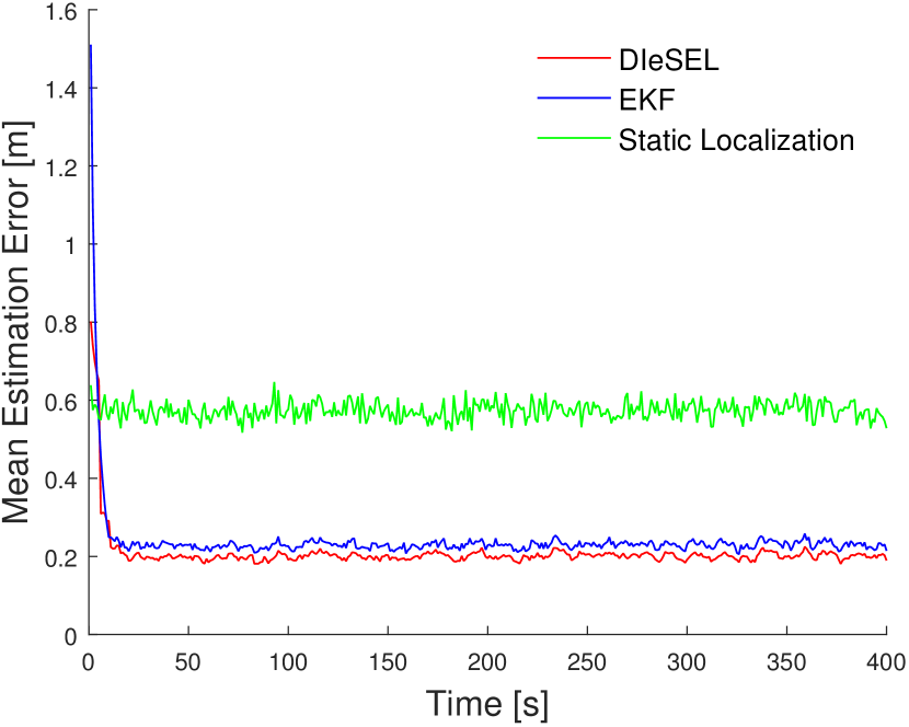
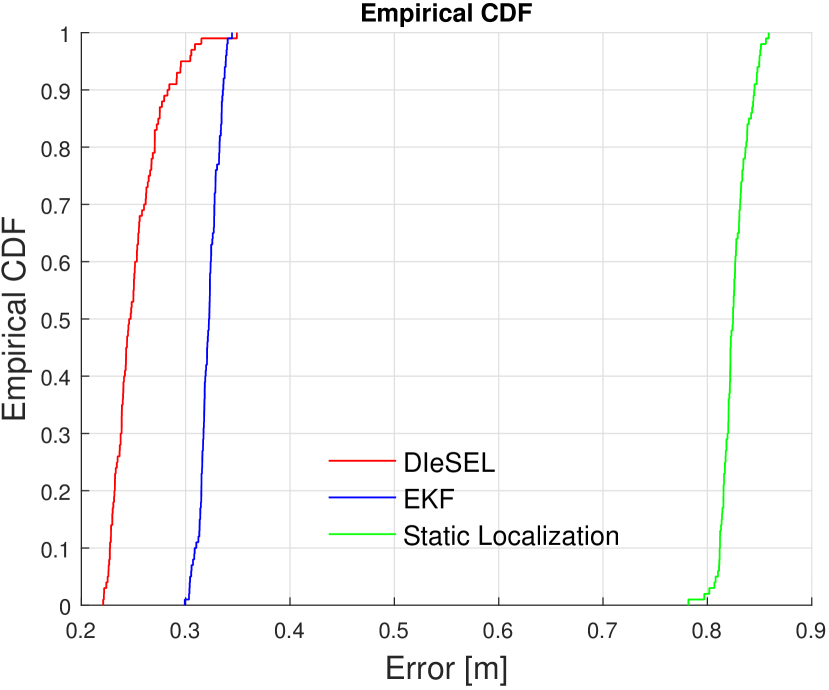
The test trajectories can be seen in Figure 1. Range noise is Gaussian with zero mean and standard deviation of 0.5m; speed is also contaminated with zero mean Gaussian noise with standard deviation of 0.01m/s. We used trajectories that could span a wide variety of AUV maneuvers: the lawnmowing, the lap and the 3D helix. Both the EKF and DIeSEL are initialized with a random position around the true initial point with a standard deviation of 2m. Figure 2 depicts the mean estimation error along the lap trajectory. We can observe that the DIeSEL error has a smaller transient and follows the trajectory with smaller value than the centralized EKF. Also, we can see that static range-only localization fares worse; this phenomenon is not unexpected: static range-only localization does not take advantage of the information of velocities and motion continuity.

Figure 2: Mean error throughout the lap trajectory. The static range-only localization method has the worst performance of the benchmark, motivated by the meagre data requirements, and by not considering motion in time. The EKF has a larger transient, and after 20 sec of the operation’s onset, DIeSEL’s error is already below the plateau of the EKF error of estimation, even when well tuned.

The normalized error per vehicle, per number of points in the trajectory is also quite revealing: Figure 3 shows that, albeit using less parameters, and being distributed, DIeSEL outperforms the EKF. In agreement with the plot in Figure 2, the comparison of empirical CDFs of the velocity- and motion-aware EKF and DIeSEL, and the static range-only localization shows the advantage of incorporating this available information.

Figure 3: Empirical CDF for the lap experiment with 100 Monte Carlo trials. The error is averaged per vehicle and per number of trajectory points. Using fewer parameters, the distributed DIeSEL algorithm outperforms the centralized EKF. Both outperform the optimization based static range-only localization.

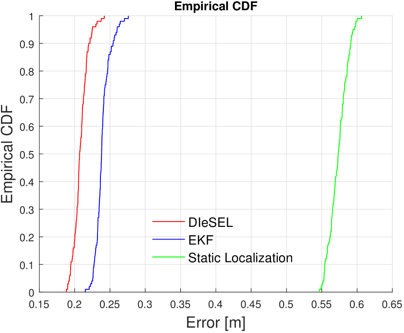
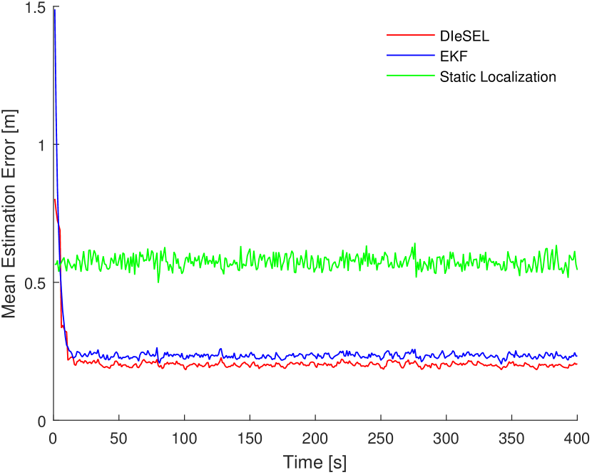
We performed the same numerical analysis for the lawnmowing trajectory. The mean estimation error depicted in Figure 4 confirms the findings for the lap. The empirical CDF in Figure 5 agrees with the corresponding results in the lap trials.

Figure 4: Mean error throughout the lawnmowing trajectory, averaged through 100 Monte Carlo trials. The static range-only localization method has, still, the worst performance of the benchmark. DIeSEL has the steepest response and the best mean estimation error.

Figure 5: Empirical CDF for 100 Monte Carlo trials on the lawnmowing trajectory. DIeSEL is the more precise algorithm, while static range-only localization fares the worst. The centralized EKF, when well tuned, can achieve at most the second best result.

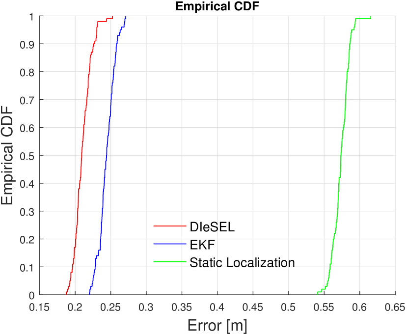
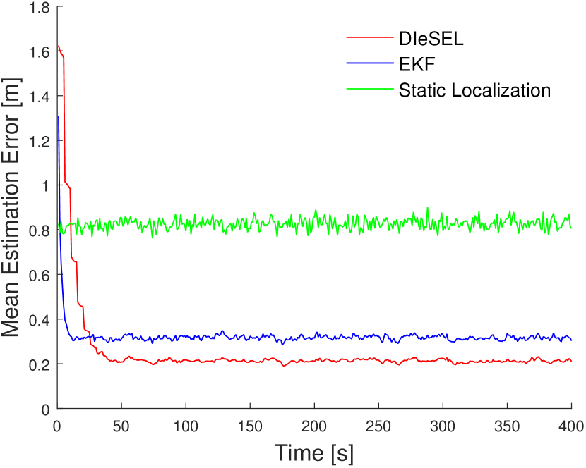
The results for the 3D helix also support the 2D results of our DIeSEL algorithm: Figure 6 shows a better tracking error, and the empirical CDF for 100 Monte Carlo trials in Figure 7 exhibits a more remarkable advantage of DIeSEL in terms of precision, when compared with the centralized EKF and static range-only localization.

Figure 6: Mean error throughout the helix trajectory. The EKF has a steepest response, mainly because the best parameter configuration weights much more the model than the measurements, so they are considered in a very low proportion in the estimation process. DIeSEL has the best trajectory following error.

Figure 7: Empirical CDF for the helix trajectory showing the averaged error on the number of vehicles and trajectory length. The distributed algorithm DIeSEL outperforms both the centralized EKF and static localization.

VI Final remarks

DIeSEL aims at precisely — and distributedly — localizing a moving network of agents in a GPS-denied environment, using a generic kinematic motion model, less dependent on the specific hardware available than the usual filtering approaches. The proposed algorithm optimizes the maximum likelihood estimation problem considering noisy Gaussian range measurements, providing a stable and convergent sequence of iterates. DIeSEL’s performance in numerical trials indicates that the performance is resilient to the choice of trajectory and has a fast transient; also the tracking error is smaller than a finely tuned centralized EKF, whereas DIeSEL worked out of the box with a small time window. With no other parameter to tune than a time window, the proposed DIeSEL algorithm finds the most precise position of agents in a cooperative network in the set of benchmark algorithms.

References

- [1] H. Al-Khatib, G. Antonelli, A. Caffaz, A. Caiti, G. Casalino, I. B. de Jong, H. Duarte, G. Indiveri, S. Jesus, K. Kebkal et al., “The widely scalable mobile underwater sonar technology (WiMUST) project: an overview,” in OCEANS 2015-Genova. IEEE, 2015, pp. 1–5.
- [2] B. C. Pinheiro, U. F. Moreno, J. T. B. de Sousa, and O. C. Rodríguez, “Kernel-function-based models for acoustic localization of underwater vehicles,” IEEE Journal of Oceanic Engineering, vol. PP, no. 99, pp. 1–16, 2016.
- [3] H. J. Rad, T. Van Waterschoot, and G. Leus, “Cooperative localization using efficient kalman filtering for mobile wireless sensor networks,” in Signal Processing Conference, 2011 19th European. IEEE, 2011, pp. 1984–1988.
- [4] Y. Shang, W. Rumi, Y. Zhang, and M. Fromherz, “Localization from connectivity in sensor networks,” Parallel and Distributed Systems, IEEE Transactions on, vol. 15, no. 11, pp. 961 – 974, Nov. 2004.
- [5] P. Biswas, T.-C. Liang, K.-C. Toh, Y. Ye, and T.-C. Wang, “Semidefinite programming approaches for sensor network localization with noisy distance measurements,” Automation Science and Engineering, IEEE Transactions on, vol. 3, no. 4, pp. 360 –371, Oct. 2006.
- [6] P. Oğuz-Ekim, J. Gomes, J. Xavier, and P. Oliveira, “Robust localization of nodes and time-recursive tracking in sensor networks using noisy range measurements,” Signal Processing, IEEE Transactions on, vol. 59, no. 8, pp. 3930 –3942, Aug. 2011.
- [7] G. Calafiore, L. Carlone, and M. Wei, “Distributed optimization techniques for range localization in networked systems,” in Decision and Control (CDC), 2010 49th IEEE Conference on, Dec. 2010, pp. 2221–2226.
- [8] C. Soares, J. Xavier, and J. Gomes, “Distributed, simple and stable network localization,” in Signal and Information Processing (GlobalSIP), 2014 IEEE Global Conference on, Dec 2014, pp. 764–768. [Online]. Available: http://bit.ly/SimpleStable14
- [9] S. Schlupkothen, G. Dartmann, and G. Ascheid, “A novel low-complexity numerical localization method for dynamic wireless sensor networks,” IEEE Transactions on Signal Processing, vol. 63, no. 15, pp. 4102–4114, Aug 2015.
- [10] C. Soares, J. Gomes, B. Ferreira, and J. P. Costeira, “LocDyn: Robust distributed localization for mobile underwater networks,” 2017, submitted. [Online]. Available: http://bit.ly/LocDynCS
- [11] A. Beck and Y. Eldar, “Sparsity constrained nonlinear optimization: Optimality conditions and algorithms,” SIAM Journal on Optimization, vol. 23, no. 3, pp. 1480–1509, 2013. [Online]. Available: http://dx.doi.org/10.1137/120869778