Multi-view pose estimation with mixtures-of-parts and adaptive viewpoint selection

Abstract

We propose a new method for human pose estimation which leverages information from multiple views to impose a strong prior on articulated pose. The novelty of the method concerns the types of coherence modelled. Consistency is maximised over the different views through different terms modelling classical geometric information (coherence of the resulting poses) as well as appearance information which is modelled as latent variables in the global energy function. Moreover, adequacy of each view is assessed and their contributions are adjusted accordingly. Experiments on the HumanEva and UMPM datasets show that the proposed method significantly decreases the estimation error compared to single-view results.

This paper is a preprint of a paper submitted to IET Computer Vision. If accepted, the copy of record will be available at the IET Digital Library.

1 Introduction

Human pose estimation is a building block in many industrial applications such as human-computer interaction, motion capture systems, etc. Whereas the problem has been almost solved for easy instances, such as cooperative settings in close distance and depth data without occlusions, other realistic configurations still present a significant challenge. In particular, pose estimation from RGB input in non-cooperative settings remains a difficult problem.

Methods range from unstructured and purely discriminative approaches in simple tasks on depth data, which allow real-time performance on low-cost hardware, up to complex methods imposing strong priors on pose. The latter are dominant on the more difficult RGB data but also increasingly popular on depth. These priors are often modelled as kinematic trees (as in the proposed method) or, using inverse rendering as geometric parametric models (see section 2 for related works).

In this paper, we leverage the information from multiple (RGB) views to impose a strong prior on articulated pose, targetting applications such as video surveillance from multiple cameras. Activity recognition in this context is frequently preceded by articulated pose estimation, which — in a non-cooperative environment such as surveillance — can strongly depend on the optimal viewpoint. Multi-view methods can often increase robustness w.r.t. occlusions.

In the proposed approach, kinematic trees model independent pose priors for each individual viewpoint, and additional terms favour consistency across views. The novelty of our contribution lies in the fact that consistency is not only forced geometrically on the solution, but also in the space of latent variables across views.

More precisely, a pose is modelled as mixtures of parts, each of which is assigned to a position. As in classical kinematic trees, deformation terms model relative positions of parts w.r.t. neighbours in the tree. In the lines of 262_yangramanan2013 , the deformations and the appearance terms depend on latent variables which switch between mixture components. This creates a powerful and expressive model with low-variance mixture components which are able to model precise relationships between appearance and deformations. Intuitively, and as an example, we could imagine relative positions of elbow and forearm to depend on a latent variable, which itself depends on the appearance of the elbow. It is easy to see that a stretched elbow requires a different relative position than a bent elbow.

In the proposed multi-view setting, positions, as well as latent variables, are modelled for each individual view. A global energy term favours a consistent pose over the complete set of views, including consistency of the latent part type variables which select mixture components. Here the premise is that appearance may certainly differ between viewpoints, but that a given pose is translated into a subset of consistent latent mixture components which can be learned.

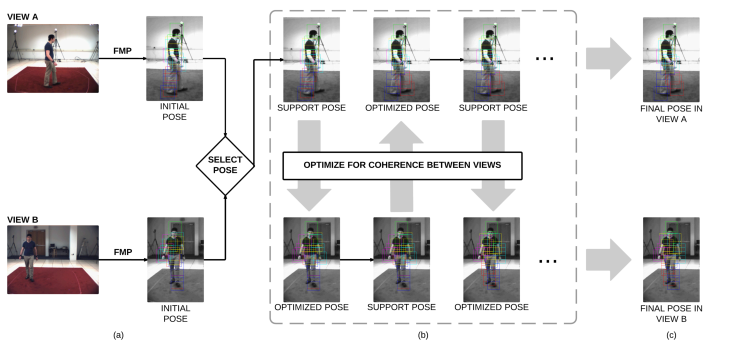
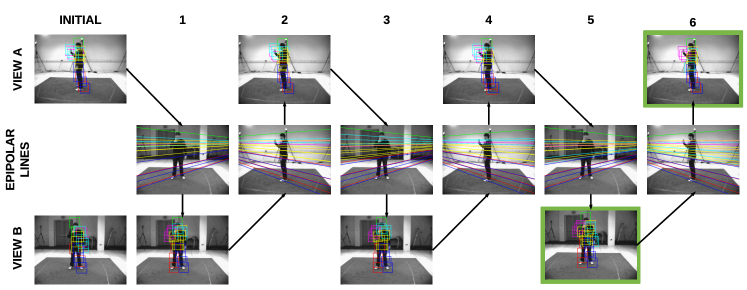
An overview of the proposed method can be seen in Fig. 1 which depicts the iterative nature of the multi-view pose estimation process. Basically, one of the single-view estimations is selected as the support pose and provides additional information to the other view. On each iteration, support and target poses are swapped so that both predictions improve over iterations. The optimisation loop continues until convergence, where a final pose is produced for each view.

As a summary, our main contributions are the following:

• We propose a global graphical model over multiple views including multiple constraints: geometrical constraints and constraints over the latent appearance space.

• We propose an iterative optimization routine.

• We introduce an adaptive viewpoint selection method, which removes viewpoints if the expected error is too high.

Figure 1: Overview of the model: a) Initial pose estimation running the single-view model on each view separately. The pose with the highest confidence score is selected as the support pose. b) Joint estimation loop with geometrical and appearance constraints provided by support pose. The newly obtained pose becomes the support pose at the end of each iteration and provides constraints for the other view. c) After convergence, the last two poses are returned as the final results. Best viewed in colour.

2 Related Work

Human pose estimation from RGB images has received increasing attention, we therefore restrict this section by excluding techniques that exploit depth images and focus on part-based models, generative and discriminative probabilistic models, tracking methods and deep neural networks.

Pictorial structures (PS) — are a dominant family of models. Based on the original idea in 250_pictorialstructures , they model an object as a combination of parts related to a star-shaped or tree-shaped structure and deformation costs. The problem is formulated as an energy function with terms for appearance similarity plus deformation terms between parts 319_sappJordanTaskar ; 315_dantone_pami2014 . Although efficient for inference, tree-structured models are known to suffer from the double-counting problem, especially for limb parts. To address this issue loopy constraints are commonly used, but they require diverse approximate inference strategies 331_NIPS2007_3271 ; 323_Zhang_2015_ICCV ; 268_cherian_2014_CVPR . The relationship between the non-adjacent body parts is discussed in 257_pishchulin_2013_CVPR where a fully-connected model is proposed. Due to mid-level representations conveyed by poselets, unary and binary terms are updated during test time and the model is reduced to a classical PS, which can be solved directly. 269_kiefel2014eccv proposes a PS-inspired model, with binary random variables for each part, they model the presence and absence for every position, scale and orientation. However, this results in a high number of variables which forces them to approximate inference.

Flexible Mixtures of Parts (FMP) — have been introduced by 262_yangramanan2013 , to tackle the limited expressiveness of tree-shaped models. Instead of orientations of parts, they proposed mixtures, which are obtained by clustering appearance information. A detailed review of the method can be found at section 3. Among extensions, 254_Eichner2013 proposed appearance sharing between independent samples to cluster similar background and foregrounds. 267_wang_2014_CVPR presented a method to estimate 3D pose from a single image where they use FMP and camera parameter estimation, in conjunction with anthropomorphic constraints. 292_cho_spl2015 proposed an improvement by aggregation of multiple hypotheses from the same view using kernel density approximation.

Multi-view settings — allow various methods to emerge, particularly for 3D pose estimation. 284_sigal2011 proposed a generalised version of PS, which also exploits temporal constraints. They employ graphs spanning multiple frames and inference is performed with non-parametric belief propagation. Among 3D extensions of PS, the burden of the infeasible 3D search space is handled by reducing it with discretisation 279_burenius2013 , supervoxels 301_schick2015 , triangulation of corresponding body parts from different viewpoints 314_belagiannis2015 or by using voxel-based annealing particle filtering 302_cantonferrer2009 . Recently, 300_zuffi2015 proposed a strategy similar to 3D-PS, but with a realistic body model, and inference is carried out with particle-based max-product belief propagation. Inferring 3D pose from multiple 2D poses is also common, with various underlying strategies such as hierarchical shape matching 287_hoffmanAndGavrila , random forests 280_kazemi2013 and optical flow 285_puwein2014 . 275_aminbmvc2013 introduced a scheme where PS is employed to estimate 2D poses, then incorporates them to obtain a 3D pose with geometrical constraints, colour and shape cues. Although being somewhat analogous to our proposition, 275_aminbmvc2013 does not consider cases where some viewpoints are more beneficial than others, which we leverage with adaptive viewpoint selection.

Temporal strategies — are commonly used for pose estimation and articulated tracking from videos. Using spatiotemporal links between the individual parts of consecutive frames seems promising, but intractability issues arise. To this end, 268_cherian_2014_CVPR opt for approximation with distance transform felzenszwalb2012distance . 323_Zhang_2015_ICCV reduce the graph by combining symmetrical parts of human body and generating part-based tracklets for temporal consistency. 325_Nie_2015_CVPR uses a spatiotemporal And/Or Graph to represent poses where only temporal links exist between parts. Recently 326_ParkRamanan_2015_CVPR proposed synthesising hypotheses by applying geometrical transformations to initially annotated pose and match next frame with the nearest neighbour search.

Discriminative approaches — learn a direct mapping from feature space to pose, often by avoiding any explicit body models (although models can be integrated). Silhouettes 329_agarwal-triggs_pami06 and edges 309_bo2008 are frequently used as image features in conjunction with learning strategies for probabilistic mapping, such as regression 329_agarwal-triggs_pami06 , Gaussian Processes 294_urtasun2008 and mixtures of Bayesian Experts 331_NIPS2007_3271 . Previous work shows that these approaches are usually computationally efficient and perform well in controlled environments, but they are highly dependent on the training data and therefore tend to generalise poorly in unconstrained settings.

Deep neural networks — have received remarkable attention recently which inevitably affected the pose estimation challenge. 253_ouyang_2014_CVPR address the problem by first obtaining 2D pose candidates with PS, then utilising a deep model the determine the final pose. 324_Fan_2015_CVPR feeds both local patches and their holistic views into the Convolutional Neural Networks (CNN), while 321_yannlecunNIPS2014 proposes a new architecture where deep CNNs are used in conjunction with Markov Random Fields. 263_toshev_2014_CVPR on the other hand, follow a more direct approach and employ a cascade of Deep Neural Network regressors to handle the pose estimation task. ChenYuille2014 uses a kinematic tree, where the same deep network learns unary terms as well as data dependent binary terms. Similar to our adaptive viewpoint selection scheme, predicting the estimation error during test time is explored by 466_Carreira_2016_CVPR ; however they employ a CNN to learn iterative corrections that converge towards the final estimation. Part mixtures is adopted in 471_Yang_2016_CVPR ; 465_Chu_2016_CVPR , where message passing is implemented as additional layers. State-of-the-art results on single-view benchmarks are achieved by 479_newell2016_ECCV , where multiple hourglass layer modules are stacked end-to-end.

Our method is based on FMP, which allows imposing a strong prior on pose, generalising it to multiple views. Compared to existing multi-view approaches, our method is not restricted to geometric coherence terms. We enforce coherence also in the space of latent variables (the mixture component selectors), which further improves performance. Additionally, we leverage the consistency between views by predicting the fitness of each view during test time.

3 Single view pose estimation

In the lines of 262_yangramanan2013 , an articulated pose in a single 2D image is modelled as a flexible mixture of parts (FMP). Related to deformable part models introduced by 147_Felzenszwalb_pami2010 , part-based models for articulated pose estimation are classically tree structured. Similarly, our model is a kinematic tree on which a global energy is defined including data attached unary terms and pairwise terms acting as a prior on body pose. The underlying graph is written as $G=(V,E)$, where vertices are parts and edges are defined on adjacency between parts.

Let $p_{i}=(x,y)$ be the pixel coordinates for part $i\in\{1,\ldots,K\}$ in image $I$. The values of $p_{i}$ are the desired result values over which we would like to optimise. Additional latent variables $t_{i}\in\{1,\ldots,T\}$ model a type of this part, which allows to model terms in the energy function for given types, effectively creating a powerful mixture model. In practice, the part types are set to clusters of appearance features during training time. In the single-view version, the energy function corresponds to the one given in 262_yangramanan2013 . Defined over a full pose $p=\{p_{i}\}$, input image $I$ and latent variables $t=\{t_{i}\}$, it is given as follows:

$$\begin{array}[]{ll}S(I,p,t)&=\sum_{i\in V}w_{i}^{t_{i}}\phi(I,p_{i})+\sum_{ij\in E}w_{ij}^{t_{i},t_{j}}\psi(p_{i}-p_{j})\\[5.0pt] &+\sum_{i\in V}b_{i}^{t_{i}}+\sum_{ij\in E}b_{ij}^{t_{i},t_{j}}\end{array}$$ (1)

The expression in the first sum corresponds to data attached terms, where $\phi(I,p_{i})$ are appearance features extracted at $p_{i}$ (HoG, see section 7). Note that the corresponding trained parameters $w_{i}^{t_{i}}$ depend on the latent part type $t_{i}$.

The pairwise terms in the next expression model the prior over body pose using a classical second degree deformation $\psi(p_{i}-p_{j})=[dx\ dx^{2}\ dy\ dy^{2}]^{T}$ where $dx=x_{i}{-}x_{j}$ and $dy=y_{i}{-}y_{j}$. They control the relative positions of the parts and act as a “switching” spring model, the switching controlled by the latent part types $t_{i}$.

The last two sums define a prior over part types including unary part type biases $b_{i}^{t_{i}}$ and pairwise part type terms $b_{ij}^{t_{i},t_{j}}$.

Although scale information is not specified in the equations, a pyramid is used in the implementation to address the various sizes of the subjects in the image. Inference in this model (and in our generalisation to multi-view problems) will be addressed in section 6.

(a)

(b)

(c)

Figure 2: Illustration of the learned multi-view consistency term over latent appearance (part types). The picture shows HoG filters of the same part (the shoulder). Filter pair (a – b) has been learned to be highly compatible (eventually across different viewpoints), whereas compatibility of pair (a – c) has been learned to be low, according to training data.

4 Multi-view pose estimation

We generalise the single-view model to multiple views and show that geometrical consistency constraints can be leveraged to improve estimation quality. Without loss of generality let us fix the number of views to two and consider a setup with calibrated cameras. In this case, a global energy function models the pose quality over a pair views $A$ and $B$, taking as input images $I^{A}$ and $I^{B}$ and estimating pose variables $p^{A}$ and $p^{B}$ while additionally optimising over latent part types $t^{A}$ and $t^{B}$:

$$\begin{array}[]{ll}S(I^{A},I^{B},p^{A},p^{B},t^{A},t^{B})&=\\[5.0pt] S(I^{A},p^{A},t^{A})&+\ S(I^{B},p^{B},t^{B})\\[5.0pt] +\alpha\sum_{i\in V}\boldsymbol{a_{i}}\xi(p_{i}^{A},p_{i}^{B})&+\ \beta\sum_{i\in V}\boldsymbol{a_{i}}\lambda(t_{i}^{A},t_{i}^{B})\\ \end{array}$$ (2)

Here, $S$ is the single pose energy from equation 1. The two additional terms $\xi$ and $\lambda$ ensure consistency of the pose over the two views, $\alpha$ and $\beta$ are the hyperparameters that controls the amount of influence of these terms, and $a_{i}$ are binary variables activating or deactivating consistency. All terms and symbols are described in the corresponding sections below.

4.1 Geometric constraints

Assuming temporal synchronisation, images $I^{A}$ and $I^{B}$ show the same articulated pose from two different viewpoints, which can be exploited. In particular, given calibrated cameras, points in a given view correspond to epipolar lines in the second view. The geometric term $\xi$ leverages this as follows:

$$\xi(p_{i}^{A},p_{i}^{B})=-d(p_{i}^{A},e(A,p_{i}^{B}))-d(p_{i}^{B},e(B,p_{i}^{A}))$$ (3)

where $e(A,p_{i}^{B})$ is the epipolar line in view $A$ of point $p_{i}$ in view $B$ and $d$ is the Euclidean squared distance between a point and a line. Thus, geometric constraints translate as additional energy to particular locations for both views in the global energy function.

4.2 Appearance constraints

The geometric constraints above are imposed on the solution (positions $p_{i}$). The term $\lambda$ adds additional constraints on the latent part type variables $t_{i}$, which further pushes the result to consistent solutions. Recall that the latent variables are clusters in feature space, i.e. they are related to types of appearance. Appearances might, of course, be different over views as a result of the deformation due to viewpoint changes. However, some changes in appearances will likely be due to the viewpoint change, whereas others will not. Intuitively, we can give the example of an open hand in view $A$, which will certainly have a different appearance in view $B$; however, the image will not likely be the one of a closed hand.

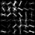
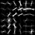
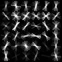
We model these constraints in a non-parametric way as a discrete distribution learned from training data, i.e. $\lambda(t_{i}^{A},t_{i}^{B})=p(t_{i}^{A},t_{i}^{B})$ (see section 5). Figure 2 illustrates this term using three filter examples shown for the learned model of part right shoulder. The $\lambda$ term is high between (2a) and (2b), but low between (2a) and (2c). Intuitively, (2a) and (2b) look like the same 3D object seen from different angles, whereas (2a) and (2c) do not.

4.3 Adaptive viewpoint selection

Geometric and appearance constraints rely on the accuracy of the initial single-view pose estimates. In certain cases, the multi-view scheme can propagate poorly estimated part positions over views, eventually deteriorating the multi-view result. To solve this problem, we would like to estimate beforehand, whether an additional view can contribute, i.e. increase performance, or whether it will deteriorate good estimations from a better view.

We propose an adaptive viewpoint selection mechanism and introduce a binary indicator vector (over parts) that switches on and off geometric and appearance constraints for each part during inference. If an indicator is switched off for a part, then the support pose does not have an effect on the optimised pose for this part. The binary indicator vector $\boldsymbol{a}$ is given as follows:

$$\boldsymbol{a}_{i}=\left\{\begin{array}[]{cc}0&\textrm{if }\sigma_{i}(p^{A},\theta)>\tau_{i}\ \textrm{or }\sigma_{i}(p^{B},\theta)>\tau_{i}\\ 1&\textrm{else}\\ \end{array}\right.$$ (4)

where $\tau_{i}$ is a threshold obtained from median part errors on the training set and $\sigma_{i}(p^{A},\theta)$ is a function with parameters $\theta$ that estimates the expected error committed by the single-view method for part $i$, given an initial estimate of the full pose $p^{A}$.

$\sigma$ is a mapping learned as a deep CNN taking image tiles cropped around the initial (single-view) detection $p^{A}$ as input. Training the network requires to minimise a loss over part estimation errors, i.e. an error over errors, as follows:

$${\min_{\theta}||\ \sigma(p^{A},\theta)-{\mathbf{e}}\ ||_{2}}$$ (5)

where ${\mathbf{e}}$ is the vector of ground truth errors obtained for the different parts by the single-view method, and $||\cdot||_{2}$ is the $L_{2}$ norm which is here taken over a vector holding estimations for individual parts. $\theta$ are the parameters of the deep network.

We argue that such a network is suitable to anticipate whether an individual part is useful for multi-view scheme, by implicitly learning multi-level features from an image tile. For example, self-occluded parts or other poor conditions would most likely to be associated with high error rates, whereas unobstructed views would yield low errors. Thresholding the output of the network, namely the error estimations ${\sigma}_{i}$, can provide the decision whether the support view has an influence for part $i$ or not.

5 Training

Single-view parameters

Appearance coefficients $w_{i}^{t_{i}}$, deformation coefficients $w_{ij}^{t_{i},t_{j}}$ and part type prior coefficients $b_{i}^{t_{i}}$ and $b_{ij}^{t_{i},t_{j}}$ are learned as in 262_yangramanan2013 : we proceed by supervised training with positive and negative samples, where the optimisation of the objective function is formulated as a structural SVM. Part type coefficients are learned w.r.t. their relative positions to their parents by clustering. This mixture of parts approach ensures the diversity of appearances of part types where their appearance is associated with their placement with reference to their parents; for example a left-oriented hand is usually seen on the left side of an elbow, while a upward facing hand is likely to occur above an elbow.

Consistency parameters

The discrete distribution $\lambda(t_{i}^{A},t_{i}^{B})=p(t_{i}^{A},t_{i}^{B})$ related to the appearance constraints between views is learned from training data as co-occurrences of part types between the viewpoint combinations. We propose a weakly-supervised training algorithm which supposes annotations of the pose (positions $p_{i}$) only, and which does not require ground truth of part types $t_{i}$. In particular, the single-view problem is solved on the images of two different viewpoints and the resulting poses are checked against the ground truth poses. If the error is small enough, the inferred latent variables $t_{i}$ are used for learning. The distribution $p(t_{i}^{A},t_{i}^{B})$ is thus estimated by histogramming eligible values for $t_{i}^{A}$ and $t_{i}^{B}$. Fig 2 shows an example of learned filters and their compatibility.

The hyper-parameters $\alpha$ and $\beta$ weighting the importance of the consistency prior are learned through cross-validation over a hold-out set (see section 7).

Viewpoint selection parameters

As seen in Section 4.3, $\sigma$ is a mapping that estimates error of a single-view pose estimation, given an image tile cropped around the bounding box. To determine $\sigma$, we use regression of the expected error and train a deep CNN. We use a VGG-16 network 500_SimonyanVGG2014_ICLR pre-trained on ImageNet and remove all the top fully connected layers and replace them with a single small hidden layer for regression. We finetune the last convolutional block of VGG and learn the weights of the newly added fully connected layers with augmented data (see section 7 for further details).

Figure 3: Illustration of the iterative optimisation process. The first and last rows are two respective viewpoints, the middle row shows epipolar lines overlaid over the respective viewpoint. Diagonal arrows show the pose that the epipolar lines are based on. Each column is an iteration and vertical arrows shows the resulting pose and epipolar lines used in joint estimation. Final poses are marked with green borders. Best viewed in colour.

HumanEva – PCP3D scores (%) of our model trained on subject 1, evaluated on subject 1 and all subjects combined, with PCP threshold $0.5$. Performance of is compared to Flexible Mixture of Parts (FMP) 262_yangramanan2013 method. Subject Sequence FMP 262_yangramanan2013 ———— Ours ———— Geom. +App. +Adap. S1 Box 77.34 82.70 83.87 85.31 All Box 67.14 69.45 70.23 71.57 S1 Gestures 78.91 84.27 84.08 88.14 All Gestures 74.68 77.38 78.81 80.34 S1 Jog 84.91 86.75 86.70 86.86 All Jog 77.52 80.16 79.84 80.97 S1 Walking 84.65 86.71 86.50 87.68 All Walking 78.49 81.69 81.96 83.17 S1 Overall 82.02 85.43 85.49 87.24 All Overall 74.86 77.62 78.11 79.40

UMPM – PCP3D scores (%) on all sequences with PCP threshold $0.5$, compared to Flexible Mixture of Parts (FMP) 262_yangramanan2013 method. Sequence FMP 262_yangramanan2013 ———— Ours ———— Geom. +App. +Adap. Chair 74.72 78.09 77.54 79.94 Grab 74.23 76.25 77.18 81.92 Orthosyn 72.47 74.65 75.22 76.48 Table 70.30 73.49 74.18 77.86 Triangle 73.69 77.26 77.81 83.81 Overall 73.07 75.91 76.37 80.04

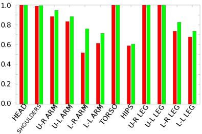
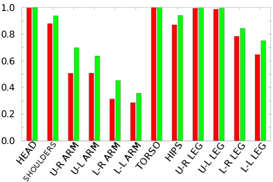
PCP3D scores (%) for all limb parts with PCP threshold $0.5$, compared to FMP262_yangramanan2013 on HumanEva and UMPM datasets.(U-L: upper left, U-R: upper right, L-L: lower left, L-R: lower right) Configuration U-R Arm U-L Arm L-R Arm L-L Arm U-R Leg U-L Leg L-R Leg L-L Leg FMP262_yangramanan2013 on HumanEva 88.4 83.4 51.8 61.4 100 100 73.6 67.9 Ours on HumanEva 94.5 88.3 76.1 71.5 100 100 82.7 73.6 FMP262_yangramanan2013 on UMPM 50.6 50.7 31.3 28.6 99.4 98.6 78.4 64.6 Ours on UMPM 69.8 63.6 45.2 35.6 99.6 99.5 84.4 75.1

6 Inference

Inference of the optimal pose pair requires maximising equation (2) over both poses $p_{i}^{A}$ and $p_{i}^{B}$ and over the full set of latent variables $t_{i}^{A}$ and $t_{i}^{B}$. Tractability depends on the structure of the graph, and on the clique functionals. Whereas the graph $G=(V,E)$ for the single-view problem (the graph underlying equation 1) is a tree, the graph of the multi-view problem contains cycles. This can be seen easily, as it is constructed as a union of two identical trees with additional edges between corresponding nodes, which are due to the consistency terms. Compared to the single-view problem, maximisation cannot be carried out exactly and efficiently with dynamic programming.

Several strategies are possible to maximise equation (2): approximative message passing (loopy belief propagation) is applicable for instance, which jointly optimises the full set of variables in an approximative way, starting from an initialisation. We instead chose an iterative scheme which calculates the exact solution for a subset of variables keeping the other variables fixed, and then alternates. In particular, as shown in figure 1, we optimise for a given view while keeping the variables of the other view (the “support view”) fixed. Removing an entire view from the optimisation space ensures that the graph over the remaining variables is restricted to a tree, which allows solving the sub-problem efficiently using dynamic programming.

Let us write $kids(i)$ for the child nodes of part $i$. The score of a part location $p_{i}$ for a given part type $t_{i}$ is computed as follows:

$$\begin{split}\textnormal{score}_{i}(t_{i}^{A},t_{i}^{B},p_{i}^{A},p_{i}^{B})&=b_{i}^{t_{i}^{A}}+w_{i}^{t_{i}}\cdot\phi(I^{A},p_{i}^{A})\\ &+b_{i}^{t_{i}^{B}}+w_{i}^{t_{i}}\cdot\phi(I^{B},p_{i}^{B})\\ &+\boldsymbol{a_{i}}(\alpha\xi(p_{i}^{A},p_{i}^{B})+\beta\lambda(t_{i}^{A},t_{i}^{B}))\\ &+\sum_{k\in kids(i)}m_{k}(t_{i}^{A},t_{i}^{B},p_{i}^{A},p_{i}^{B})\end{split}$$ (6)

with the message that part $i$ passes to its parent $j$ is defined as:

$$\begin{split}m_{i}(t_{j}^{A},t_{j}^{B},p_{j}^{A},p_{j}^{B})&=\max_{t_{i}^{A},t_{i}^{B}}\Big{[}b_{ij}^{t_{i}^{A},t_{j}^{A}}+b_{ij}^{t_{i}^{B},t_{j}^{B}}\\ &+\max_{p_{i}^{A},p_{i}^{B}}\textnormal{score}_{i}(t_{i}^{A},t_{i}^{B},p_{i}^{A},p_{i}^{B})\\ &+w_{ij}^{t_{i}^{A},t_{j}^{A}}\cdot\psi(p_{i}^{A},p_{j}^{A})+w_{ij}^{t_{i}^{B},t_{j}^{B}}\cdot\psi(p_{i}^{B},p_{j}^{B})\Big{]}\end{split}$$ (7)

As mentioned, one of the two sets $A$ and $B$ is kept constant at each time, which simplifies the equations (6, 7) to a single-view form, similar to 262_yangramanan2013 . Messages from all children of part $i$ are collected and summed with the bias term and filter response, resulting in the score for that pixel position and mixture pair. As classically done in deformable parts based models, the optimisation can be carried out with dynamic programming and the inner maximisation in equation (7) with min-convolutions (a distance transform, see felzenszwalb2012distance ).

The algorithm is initialised by solving the single-view problem independently for each viewpoint. The pose with the lowest estimated error (see section 4.3) is chosen as initial support pose, the pose of the other viewpoint being optimised in the first iteration. The iterative process is repeated on until convergence or a maximum number of iterations is reached. Optimising each sub-problem is classical, where the message passing scheme iterates from the leaf nodes to the root node. After thresholding to eliminate weak candidates and non-maximum suppression to discard similar ones, backtracking obtains the final pose.

7 Experiments

We evaluated our work on two datasets, HumanEva I 313_sigal2010humaneva and Utrecht Multi-Person Motion (UMPM) UMPM . Both datasets have been shot using several calibrated cameras. Ground truth joint locations were recorded with a motion capture system, with 20 and 15 joints, respectively.

For HumanEva set we only use three cameras (C1, C2 and C3), which are placed with 90 degrees offset. Three subjects (S1, S2 and S3) perform following activities: walking, boxing, jogging, gestures and throw-catch. There are three takes for each sequence, used for training, validation and test. Since the creators of HumanEva favour online evaluation, original test set does not contain ground truth joint positions. Following 275_aminbmvc2013 , we divided the original training set into training and validation sets and used the original validation set for testing. All hyper-parameters have been optimised over our validation set.

For UMPM set, all available cameras (F, L, R and S) were used. We considered all available sequences with one subject, which includes object interactions such as sitting on a chair, picking up a small object, leaning and lying on a table. The training, validation and test partitions were divided using 60%, 20% and 20% of the all available data, respectively. The HumanEva test set consists of 4493 images per camera, while UMPM test set has 6074 images per camera. The number of distinct images used in the tests sums up to 13479 and 24296, respectively.

Since our model is trained with 26 parts, we used a linear function to convert our box centres to the 20 joint locations for HumanEva and 15 joints locations for UMPM.

The data attached terms $\phi(.,.)$ in this work were based on HoG features from 169_HOG_dalaltriggs . Other features are possible, in particular learned deep feature extractors as in ChenYuille2014 or NeverovaArxiv2016handpose ; FourureNeurocomp2017 . This does not change the setup, and can be performed with finetuning of a pre-trained model for this case, where the amount of training data is relatively low.

We evaluate our multi-view approach against the single-view method given in 262_yangramanan2013 . We use two poses as input and evaluate on one of these two poses, varying over multiple configurations.

Parameters of the single-view model (Eq. 1) are learned on all activities of S1 for HumanEva. We took 100 frames with equal time intervals for every activity from three cameras for training, which sums up to 1500 images. The remainder of the data was set as the validation set. For UMPM, nearly 400 consecutive frames for each sequence were used as positive samples. As for the negative samples, background images from corresponding datasets were used in addition to the INRIA Person Database 169_HOG_dalaltriggs . Hyper-parameters $\alpha$ and $\beta$ of equation (2) were learned on validation sets.

(a) HumanEva, S1, all sequences

(b) UMPM, all sequences

Figure 4: PCP3D scores (%) for individual parts obtained by FMP262_yangramanan2013 (red) and ours (green) on both datasets. (U-L: upper left, U-R: upper right, L-L: lower left, L-R: lower right)

Figure 5: Qualitative comparison of all three subjects performing various activities from different viewpoints. Top: poses obtained with the single-view model 262_yangramanan2013 . Bottom: poses obtained with multi-view pose estimation. Best viewed in colour.

(a) HumanEva, S1, all sequences

(b) UMPM, all sequences

Figure 6: PCP3D curves (%) obtained by FMP262_yangramanan2013 (red) and ours (green) on both datasets, as a function of PCP threshold $\gamma$, which controls the ratio of the detected part segments to the ground truth to be considered correctly detected, as defined in Eq. (8).

To learn the weights of the error estimating CNN $\sigma_{i}(\cdot)$, training data sets were augmented with horizontal flip, Gaussian blur and additive noise. As mentioned earlier, we used a finetuned version of VGG-16 500_SimonyanVGG2014_ICLR model using pre-trained weights on ImageNet to estimate the part-based error of the single-view pose. We removed the fully connected layers and introduced our top model with a hidden layer of 1024 nodes, an output layer of $K$ nodes and parametric ReLU as non-linearity. First, weights of the complete VGG-16 network were frozen so that they are unaffected by the backpropagation and weights of the top model were roughly learnt with a high learning rate. Then, the top model were initialised with these weights, and the last convolutional blocks (namely the last three conv3-512 layers) were unfrozen for finetuning. We preferred stochastic gradient descent as optimisation algorithm with small learning rate to ensure that the weights of the last convolutional block are marginally updated. To prevent overfit to augmented data sets we applied strong regularisation and also employed Dropout 501_SrivastavaDropout2014_JMLR with a probability of 0.5.

For each multi-view arrangement, i.e. pair combinations of cameras, two pose estimations are produced. Since each view belongs to several multi-view arrangements, we end up with several pose candidates for the same viewpoint, e.g. we obtain two pose candidate for C1, once from the C1-C2 pair and once from the C3-C1 pair. These candidates are simply averaged and obtained 2D poses are triangulated non-linearly to obtain 3D pose for a single time frame. Following the literature on 3D pose estimation 279_burenius2013 ; 301_schick2015 we use the percentage of correctly detected parts in 3D (PCP3D), which is calculated as

$$\frac{\lVert\hat{s}_{n}-s_{n}\rVert+\lVert\hat{e}_{n}-e_{n}\rVert}{2}\leq\gamma\lVert\hat{s}_{n}-\hat{e}_{n}\rVert$$ (8)

where $s_{n}$ and $e_{n}$ are the estimated start and end 3D coordinates of the $n$’th part segment, and $\hat{s}_{n}$ and $\hat{e}_{n}$ are the ground truth 3D coordinates for the same part segment. By convention we take $\gamma=0.5$ in all our computations, unless specified otherwise.

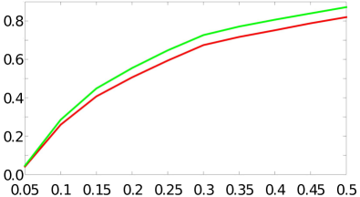
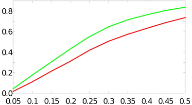
Performances — are shown in Table 5 as PCP3D scores on train subject S1 only and over all subjects; while table 5 shows PCP3D scores on UMPM test set. We provide three versions: geometric constraints only, geometric and appearance constraints combined, and both constraints with adaptive viewpoint selection. It is clear that in all cases and both data sets, the multi-view scheme significantly improves performance. Depending on the performed action, gains can be significant up to 9.2% in HumanEva and 10.1% in UMPM. The last columns of tables 5 and 5 show that the additional coherence terms decrease the error. Fig. 4 demonstrates that this error is distributed over all different parts of the body: we improve most on wrists and elbows, which are important joints for gesture and activity recognition, as seen in table 5. Plots for overall PCP3D curves w.r.t. various thresholds are also given in Fig. 6.

The adaptive viewpoint selection — effectively prevents erroneous consistency terms for certain parts dynamically, due to poor initial single-view estimations as discussed in Section 4.3, and shown in table 5.

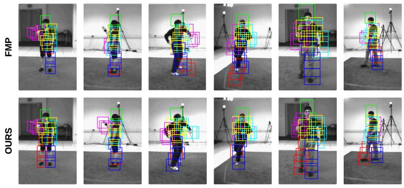
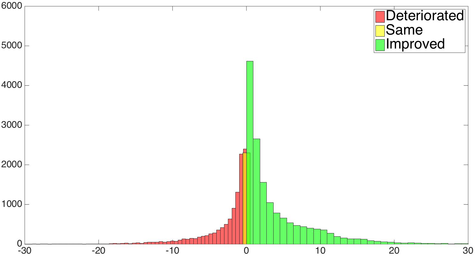
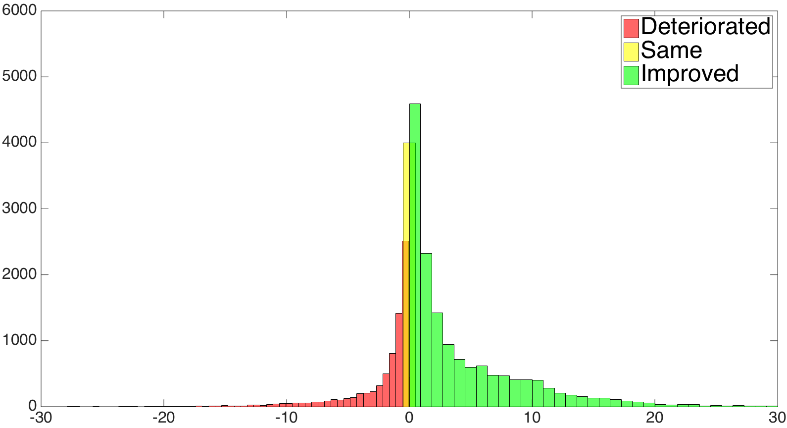
Fig. 3 depicts intermediate poses and epipolar lines throughout the course of algorithm while Fig. 5 shows several examples from the test set, where faulty poses are corrected with the multi-view approach. Note that limbs are in particular subject to correction by geometrical and appearance based constraints, since they are considerably susceptible to be mistaken for their respective counterpart. It should be also noted that in case of poor initial detections, a faulty part location can be propagated through the constraints and deteriorate a correct part estimation in other views. Performance tables show that our adaptive viewpoint selection scheme successfully prevents this by considerably decreasing the number of deterioration cases. Particularly, Fig. 7 depicts the the amount of improvements and deteriorations w.r.t the baseline, with and without the adaptive viewpoint selection scheme, which efficiently discards the erroneous single-view part detections.

Comparison to the state of the art — We compare to the original FMP 262_yangramanan2013 , to Schick et al.’s voxel carving based 3D PS method 301_schick2015 and to pre-trained Stacked Hourglass Networks (SHN) 479_newell2016_ECCV .

301_schick2015 report 78% PCP3D for HumanEva and for all sequences of S1 and S2 (ours: 83.42%) and they report 75% for UMPM and for all sequences of P1 (ours: 80.04%).

SHN 479_newell2016_ECCV requires a cropped input image that is centred around the person with specific scale requirements. Similar to our scheme, 2D poses from different views were triangulated to obtain 3D pose. Table 7 depicts our estimation performance and two versions of 479_newell2016_ECCV : First one is with unrestricted images, i.e. same input to our method; and second one with pre-processing steps that require the ground truth. Please note that the SHN heavily depends on the pre-processing, and fails if the person is not centred on image. Our method, which does not require such supervision, obtains similar or better performance to SHN with pre-processed input.

Comparison of our performance to SHN 479_newell2016_ECCV on subject 1 of HumanEva dataset, in terms of PCP3D score (%). First reported result is calculated with unrestricted images (i.e. same input for our method) which is dubbed as Standard, while the second one is calculated with cropped input images around the person with a scale requirement, which is dubbed as Pre-processed. (U-L: upper left, U-R: upper right, L-L: lower left, L-R: lower right) Body Part Ours SHN Standard SHN Pre-processed Head 100.0 7.40 25.17 Shoulders 99.47 49.08 100.0 U-R Arm 94.52 15.13 96.37 U-L Arm 88.31 45.51 98.48 L-R Arm 76.09 7.73 73.98 L-L Arm 71.53 41.88 84.54 Torso 100.0 52.58 100.0 Hips 60.63 0.0 65.52 U-R Leg 100.0 52.64 100.0 U-L Leg 100.0 51.65 100.0 L-R Leg 82.69 51.65 99.41 L-L Leg 73.58 48.15 98.15 Overall 87.24 35.28 86.80

(a) Without adaptive viewpoint selection

(b) With adaptive viewpoint selection

Figure 7: Illustration of the effect of adaptive viewpoint selection. The histograms show differences of errors (px) compared to the baseline 262_yangramanan2013 . Negative differences (red) indicate that our method performs worse, positive differences (green) indicate that our method yielded a better pose. The adaptive mechanism reduces deteriorations while keeping improvements.

Fast parallel implementation

Our implementation is based on our port of the Matlab/C++code from the single-view method by 262_yangramanan2013 to 100% pure C++, where crucial parts have also been ported to GPU processing using NVIDIA’s CUDA library. This sped up runtime from 3000ms/frame to 880ms/frame on a computer equipped with a 2.4Ghz Xeon E5-2609 processor and an NVIDIA 780 Ti GPU for the single-view algorithm (for a 172x224 image with 32 levels of down-sampling). The multi-view algorithm is slower as 5.73 iterations are performed in average before the results are stable. We are currently working on additional optimisations of computational complexity using approximative parallel implementations of the distance transform on GPUs.

8 Conclusion

We proposed a novel multi-view method to estimate articulated body pose from RGB images. Experiments show that combining appearance constraints with geometrical constraints and adaptively applying them on individual parts yields better results than the original single-view model. We also show that our algorithm performs more accurately regardless of the view combinations, and it generalises well in a way to handle unseen subjects and activities.

We plan to extend and evaluate our method in settings with three or more viewpoints, which should be straightforward. Generally, a graph modelling the possible interactions could possibly have high-order cliques, where each clique contains nodes corresponding to the possible views. In practice, it is unsure whether high-order interactions should provide more powerful constraints then (sub)-sets of pairwise constraints. A straightforward algorithm should be similar to the one proposed in the paper: optimizations are carried out over a single-view including pairwise terms involving the different (multiple) support views.

Another improvement would be the extension to a non-calibrated setting, by exploring the self-calibration and epipolar line estimation techniques, which would allow our method to be used in multi-agent robotic systems.

9 Acknowledgment

This work was partly supported by a grant of type BQR by Fondation INSA-Lyon, project CROME.

References

- [1] Yang, Y., Ramanan, D.: ‘Articulated human detection with flexible mixtures of parts’, IEEE T on PAMI, 2013, 35, (12), pp. 2878–2890
- [2] Felzenszwalb, P.F., Huttenlocher, D.P.: ‘Pictorial structures for object recognition’, IJCV, 2005, 61, (1), pp. 55–79
- [3] Sapp, B., Jordan, C., Taskar, B. ‘Adaptive pose priors for pictorial structures’. In: CVPR. (San Francisco, CA, 2010). pp. 422–429
- [4] Dantone, M., Gall, J., Leistner, C., Van.Gool, L.: ‘Body parts dependent joint regressors for human pose estimation in still images’, IEEE T on PAMI, 2014, 36, (11), pp. 2131–2143
- [5] Sigal, L., Balan, A., Black, M.J. ‘Combined discriminative and generative articulated pose and non-rigid shape estimation’. In: NIPS. (Vancouver, Canada, 2008). pp. 1337–1344
- [6] Zhang, D., Shah, M. ‘Human pose estimation in videos’. In: ICCV. (Santiago, Chile, 2015). pp. 2012–2020
- [7] Cherian, A., Mairal, J., Alahari, K., Schmid, C. ‘Mixing body-part sequences for human pose estimation’. In: CVPR. (Columbus, Ohio, 2014). pp. 2361–2368
- [8] Pishchulin, L., Andriluka, M., Gehler, P., Schiele, B. ‘Poselet conditioned pictorial structures’. In: CVPR. (Portland, Oregon, 2013). pp. 588–595
- [9] Kiefel, M., Gehler, P. ‘Human pose estimation with fields of parts’. In: ECCV. (Zurich, Switzerland, 2014). pp. 331–346
- [10] Eichner, M., Ferrari, V. ‘Appearance sharing for collective human pose estimation’. In: ACCV. (Daejeon, Korea, 2013). pp. 138–151
- [11] Wang, C., Wang, Y., Lin, Z., Yuille, A.L., Gao, W. ‘Robust estimation of 3d human poses from a single image’. In: CVPR. (Columbus, Ohio, 2014). pp. 2369–2376
- [12] Cho, E., Kim, D.: ‘Accurate human pose estimation by aggregating multiple pose hypotheses using modified kernel density approximation’, Signal Processing Letters, IEEE, 2015, 22, (4), pp. 445–449
- [13] Sigal, L., Isard, M., Haussecker, H., Black, M.J.: ‘Loose-limbed people: Estimating 3D human pose and motion using non-parametric belief propagation’, IJCV, 2011, 98, (1), pp. 15–48
- [14] Burenius, M., Sullivan, J., Carlsson, S. ‘3d pictorial structures for multiple view articulated pose estimation’. In: CVPR. (Portland, Oregon, 2013). pp. 3618–3625
- [15] Schick, A., Stiefelhagen, R. ‘3d pictorial structures for human pose estimation with supervoxels’. In: IEEE Winter Conf. on Applications of Computer Vision. (Hawaii, Hawaii, 2015). pp. 140–147
- [16] Belagiannis, V., Amin, S., Andriluka, M., Schiele, B., Navab, N., Ilic, S.: ‘3d pictorial structures revisited: Multiple human pose estimation’, IEEE T on PAMI, 2015, PP, (99), pp. 1–1
- [17] Canton.Ferrer, C., Casas, J.R., Pardas, M. ‘Voxel based annealed particle filtering for markerless 3d articulated motion capture’. In: 3DTV. (Potsdam, Germany, 2009). pp. 1–4
- [18] Zuffi, S., Black, M.J. ‘The stitched puppet: A graphical model of 3d human shape and pose’. In: CVPR. (Boston, Massachusetts, 2015). pp. 3537–3546
- [19] Hofmann, M., Gavrila, D.M. ‘Multi-view 3d human pose estimation combining single-frame recovery, temporal integration and model adaptation’. In: CVPR. (Miami, Florida, 2009). pp. 2214–2221
- [20] Kazemi, V., Burenius, M., Azizpour, H., Sullivan, J. ‘Multi-view body part recognition with random forests’. In: BMVC. (Bristol, United Kingdom, 2013).
- [21] Puwein, J., Ballan, L., Ziegler, R., Pollefeys, M. ‘Joint camera pose estimation and 3d human pose estimation in a multi-camera setup’. In: ACCV. (Singapore, 2014). pp. 473–487
- [22] Amin, S., Andriluka, M., Rohrbach, M., Schiele, B. ‘Multi-view pictorial structures for 3d human pose estimation’. In: BMVC. (Bristol, United Kingdom, 2013).
- [23] Felzenszwalb, P.F., Huttenlocher, D.P.: ‘Distance transforms of sampled functions.’, Theory of computing, 2012, 8, (1), pp. 415–428
- [24] Xiaohan.Nie, B., Xiong, C., Zhu, S.C. ‘Joint action recognition and pose estimation from video’. In: CVPR. (Boston, Massachusetts, 2015). pp. 1293–1301
- [25] Park, D., Ramanan, D. ‘Articulated pose estimation with tiny synthetic videos’. In: CVPR Workshop. (Boston, Massachusetts, 2015). pp. 58–66
- [26] Agarwal, A., Triggs, B.: ‘Recovering 3d human pose from monocular images’, IEEE T on PAMI, 2006, 28, (1), pp. 44–58
- [27] Bo, L., Sminchisescu, C., Kanaujia, A., Metaxas, D. ‘Fast algorithms for large scale conditional 3d prediction’. In: CVPR. (Anchorage, Alaska, 2008). pp. 1–8
- [28] Urtasun, R., Darrell, T. ‘Sparse probabilistic regression for activity-independent human pose inference’. In: CVPR. (Anchorage, Alaska, 2008). pp. 1–8
- [29] Ouyang, W., Chu, X., Wang, X. ‘Multi-source deep learning for human pose estimation’. In: CVPR. (Columbus, Ohio, 2014). pp. 2337–2344
- [30] Fan, X., Zheng, K., Lin, Y., Wang, S. ‘Combining local appearance and holistic view: Dual-source deep neural networks for human pose estimation’. In: CVPR. (Boston, Massachusetts, 2015). pp. 1347–1355
- [31] Tompson, J.J., Jain, A., LeCun, Y., Bregler, C. ‘Joint training of a convolutional network and a graphical model for human pose estimation’. In: NIPS. (Montreal, Canada, 2014). pp. 1799–1807
- [32] Toshev, A., Szegedy, C. ‘Deeppose: Human pose estimation via deep neural networks’. In: CVPR. (Columbus, Ohio, 2014). pp. 1653–1660
- [33] Chen, X., Yuille, A.L. ‘Articulated pose estimation by a graphical model with image dependent pairwise relations’. In: Advances in Neural Information Processing Systems 27. (Columbus, Ohio, 2014). pp. 1736–1744
- [34] Carreira, J., Agrawal, P., Fragkiadaki, K., Malik, J. ‘Human pose estimation with iterative error feedback’. In: CVPR. (Las Vegas, Nevada, 2016). pp. 4733–4742
- [35] Yang, W., Ouyang, W., Li, H., Wang, X. ‘End-to-end learning of deformable mixture of parts and deep convolutional neural networks for human pose estimation’. In: CVPR. (Las Vegas, Nevada, 2016). pp. 3073–3082
- [36] Chu, X., Ouyang, W., Li, H., Wang, X. ‘Structured feature learning for pose estimation’. In: CVPR. (Las Vegas, Nevada, 2016). pp. 4715–4723
- [37] Newell, A., Yang, K., Deng, J. ‘Stacked hourglass networks for human pose estimation’. In: ECCV. (Amsterdam, Netherlands, 2016). pp. 483–499
- [38] Felzenszwalb, P.F., Girshick, R.B., McAllester, D., Ramanan, D.: ‘Object detection with discriminatively trained part-based models’, IEEE T on PAMI, 2010, 32, (9), pp. 1627–1645
- [39] Simonyan, K., Zisserman, A.: ‘Very deep convolutional networks for large-scale image recognition’, CoRR, 2014, abs/1409.1556
- [40] Sigal, L., Balan, A.O., Black, M.J.: ‘Humaneva: Synchronized video and motion capture dataset and baseline algorithm for evaluation of articulated human motion’, IJCV, 2010, 87, (1-2), pp. 4–27
- [41] van der Aa, N.P., Luo, X., Giezeman, G.J., Tan, R.T., Veltkamp, R.C. ‘Umpm benchmark: A multi-person dataset with synchronized video and motion capture data for evaluation of articulated human motion and interaction’. In: HICV / ICCV 2011. (Barcelona, Spain, 2011). pp. 1264–1269
- [42] Dalal, N., Triggs, B. ‘Histograms of oriented gradients for human detection’. In: CVPR. vol. 1. (San Diego, CA, 2005). pp. 886–893
- [43] Neverova, N., Wolf, C., Taylor, G.W., Nebout, F.: ‘Hand pose estimation through weakly-supervised learning of a rich intermediate representation’, Pre-print: arxiv:151106728, 2015,
- [44] Fourure, D., Emonet, R., Fromont, E., Muselet, D., Neverova, N., Trémeau, A., et al.: ‘Multi-task, multi-domain learning: application to semantic segmentation and pose regression’, , 2017, 251, pp. 68–80
- [45] Srivastava, N., Hinton, G., Krizhevsky, A., Sutskever, I., Salakhutdinov, R.: ‘Dropout: A simple way to prevent neural networks from overfitting’, J Mach Learn Res, 2014, 15, (1), pp. 1929–1958