Learning Domain-Specific Word Embeddings from Sparse Cybersecurity Texts
Abstract
Word embedding is a Natural Language Processing (NLP) technique that automatically maps words from a vocabulary to vectors of real numbers in an embedding space. It has been widely used in recent years to boost the performance of a variety of NLP tasks such as Named Entity Recognition, Syntactic Parsing and Sentiment Analysis. Classic word embedding methods such as Word2Vec and GloVe work well when they are given a large text corpus. When the input texts are sparse as in many specialized domains (e.g., cybersecurity), these methods often fail to produce high-quality vectors. In this paper, we describe a novel method to train domain-specific word embeddings from sparse texts. In addition to domain texts, our method also leverages diverse types of domain knowledge such as domain vocabulary and semantic relations. Specifically, we first propose a general framework to encode diverse types of domain knowledge as text annotations. Then we develop a novel Word Annotation Embedding (WAE) algorithm to incorporate diverse types of text annotations in word embedding. We have evaluated our method on two cybersecurity text corpora: a malware description corpus and a Common Vulnerability and Exposure (CVE) corpus. Our evaluation results have demonstrated the effectiveness of our method in learning domain-specific word embeddings.
Introduction
Word embedding is a technique in Natural Language Processing (NLP) that transforms the words in a vocabulary into dense vectors of real numbers in a continuous embedding space. While traditional NLP systems represent words as indices in a vocabulary that do not capture the semantic relationships between words, word embeddings such as those learned by neural networks explicitly encode distributional semantics in learned word vectors. Moreover, through low-dimensional matrix operations, word embeddings can be used to efficiently compute the semantics of larger text units such phrases, sentences and documents (?), (?). Since effective word representations play an important role in Natural Language Processing (NLP), there is a recent surge of interests in incorporating word embeddings in a variety of NLP tasks such as Named Entity Recognition (?), (?), syntactic parsing (?), semantic relation extraction (?), (?) and sentiment analysis (?), (?), to boost their performance.
To capture the distributional semantics of words from unannotated text corpora, typical word embedding methods such as Word2Vec (?) and GloVe (?) rely on the co-occurrences of a target word and its context. Since robust inference can be achieved only with sufficient co-occurrences, this posts a challenge to applications where the domain texts are sparse. For example, traditional word embedding methods such as Word2Vec do not very perform well in highly specialized domains such as cybersecurity where important domain concepts often do not occur many times (e.g., many CVE names only occur once or twice in the entire CVE dataset). Since word embedding is an important resource for typical NLP tasks, a lack of high-quality word embeddings to capture the semantics of important domain terms and their relations may prevent the state-of-the-art NLP techniques from being adopted in processing domain-specific texts.
In a specific domain, in addition to text, sometimes there exist domain-specific knowledge resources created by domain experts to facilitate information processing. For example, in the medical domain, the UMLS or Unified Medical Language System defines and standardizes many health and biomedical vocabularies to enable interoperability between computer systems. In the cybersecurity domain, domain texts such as malware descriptions are often accompanied by a set of domain meta data. such as malware type.
In this research, we proposed a general framework to leverage diverse types of existing domain knowledge to improve the quality of word embedding when the domain texts are sparse. First, we design a flexible mechanism to encode diverse types of domain knowledge as text annotations. This allows us to design a unified framework to incorporate different types of domain knowledge. Previously, different word embedding algorithms have to be invented to incorporate different types of domain knowledge (?; ?). We have also developed a Word and Annotation Embedding (AWE) algorithm that is capable of incorporating word annotations in word embeddings. We have applied our method to two cybersecurity text corpora: a malware description corpus and a CVE corpus. We compared the performance of our system with that of a comprehensive set of general-purpose and domain-specific word embedding models. Our evaluation results demonstrate the superiority of our method. For example, our method outperformed the best baseline model by 22%-57% based on a Mean Reciprocal Rank (MRR)-based evaluation measure.
In summary, the main contributions of our work include
-
•
We present a general framework to incorporate diverse types of domain knowledge to improve the quality of domain-specific word embeddings when the input domain texts are sparse.
-
–
We propose a flexible mechanism to encode diverse types of domain knowledge such as domain vocabulary, semantic categories and semantic relations as text annotations.
-
–
We develop a novel Word and Annotation Embedding (WAE) algorithm to incorporate text annotations in word embeddings.
-
–
-
•
We have applied the proposed method to two cybersecurity datasets. Our method consistently and significantly outperformed a comprehensive set of baseline approaches in capturing important semantic relations between domain concepts.
Related Work
There is a rich body of work on learning general-purpose word embeddings (?) , (?), (?), (?), (?). Word embedding gained much popularity with the Word2Vec method (?). It includes two models: a continuous bag-of-words model (CBOW) and a skip-gram model (Skip-Gram), both learn word embeddings from large-scale unsupervised text corpora.
Since then, many extensions to Word2Vec have been proposed (?), (?), (?), (?), (?), (?), (?), (?). For example, Doc2Vec (?) is an extension of word2vec which learns vector representations for sentences and documents. Since the original work of Word2Vec uses a linear context (the words preceding and following the target word), (?) extends this by employing the syntactic contexts derived from automatically generated dependency parse-trees. These syntactic contexts were found to capture more functional similarities, while the linear contexts in the original Skip-Gram model generate broad topical similarities. In addition, (?) proposes a neural model to learn morphologically-aware word representations by combining a recursive neural network and neural language model. (?) proposes a joint representation learning method that simultaneously predicts the co-occurrences of two words in a sentence, subject to the relational constrains given by a semantic lexicon. Finally, (?) learns sentiment-specific word embeddings by considering not only the syntactic context of words but also the sentiment of words.
So far, there are only very few studies focusing on learning domain-specific word embeddings. For example, (?) uses information from a disease lexicon to generate disease-specific word embeddings. The main objective is to bring in-domain words close to each other in the embedding space while pushing out-domain words away from in-domain words. Unlike our system which can incorporate diverse types of domain knowledge, (?) only concerns whether a word is in-domain or not. To the best of our knowledge, the method we are proposing is the most comprehensive approach for training domain-specific word embeddings.
Datasets
In this research, we employ two cybersecurity datasets, a malware dataset which includes the descriptions of computer malware and a CVE dataset which includes the descriptions of common vulnerabilities and exposures in computer hardware and software.
The Malware Dataset
Malware, or malicious software, is any program or file that is harmful to a computer user. Malware can perform a variety of functions including stealing, encrypting or deleting sensitive data, altering or hijacking core computing functions and monitoring users’ computer activity without their permission. There are different types of malware. For example, a malware can be a virus, a worm, a trojan horse, a spyware, a ransomware, an adware and a scareware.
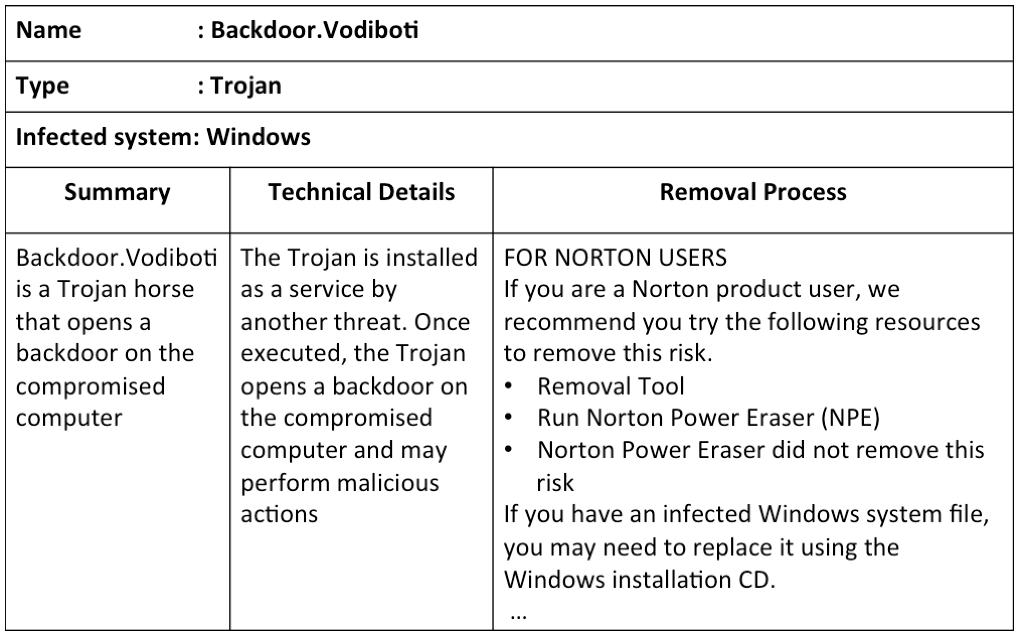
Our malware dataset is collected from two anti-virus companies: Symantec111https://www.symantec.com/ and Trend Micro222https://www.trendmicro.com/. The Symantec dataset contains 16,167 malware descriptions Each description contains three sections: summary, technical details and the removal process. In addition, each malware description also includes a set of meta data such as malware type and systems affected. The Trend Micro dataset contains 424 malware descriptions. Each description also includes three similar sections: overview, technical details and solution. It also includes similar metadata such as threat type and platform, which can be roughly mapped to malware type and systems affected used in the Symantec description. Interestingly, different security firms often adopt different naming conventions. As a result, the same malware may have different names due to different name conventions. Overall, the entire malware dataset has a total of 19, 801,192 tokens and 296, 340 unique words. Figure 1 shows the Symantec description of a recently discovered malware called Backdoor.Vodiboti.
The CVE Dataset
In computer security, a vulnerability is a flaw or weakness in security procedures, system design and implementation, or internal controls that could be exercised (accidentally triggered or intentionally exploited) and result in a security breach or a violation of the system’s security policy. Common Vulnerabilities and Exposures (CVE) is an industry standard of common names for publicly known security vulnerabilities and has been widely adopted by organizations to provide better coverage, easier interoperability, and enhanced security in managing cybersecurity systems.
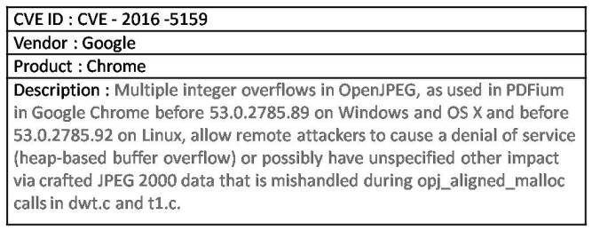
Our CVE dataset is collected from the National Vulnerability Database(NVD 333https://nvd.nist.gov/). This dataset contains detailed descriptions of 82, 871 CVEs with a total of 11, 156, 567 word tokens and 300, 074 unique word types. Each CVE description includes a CVE Identifier number, a brief description of the security vulnerability or exposure, any pertinent references (i.e., vulnerability reports and advisories) and additional metadata such as vendor, product and product version. Figure 2 shows an example of a CVE description.
Representing Knowledge as Text Annotations
Since there are diverse types of domain knowledge that might be useful to a specific application, instead of designing different algorithms to incorporate different kinds of domain knowledge, we develop a unified framework to incorporate different types of domain knowledge. To facilitate this, we propose a text annotation-based mechanism to encode different types of domain knowledge such as domain vocabulary, semantic categories and semantic relations. In the following, we use an example to illustrate how to convert different types of domain knowledge into text annotations.
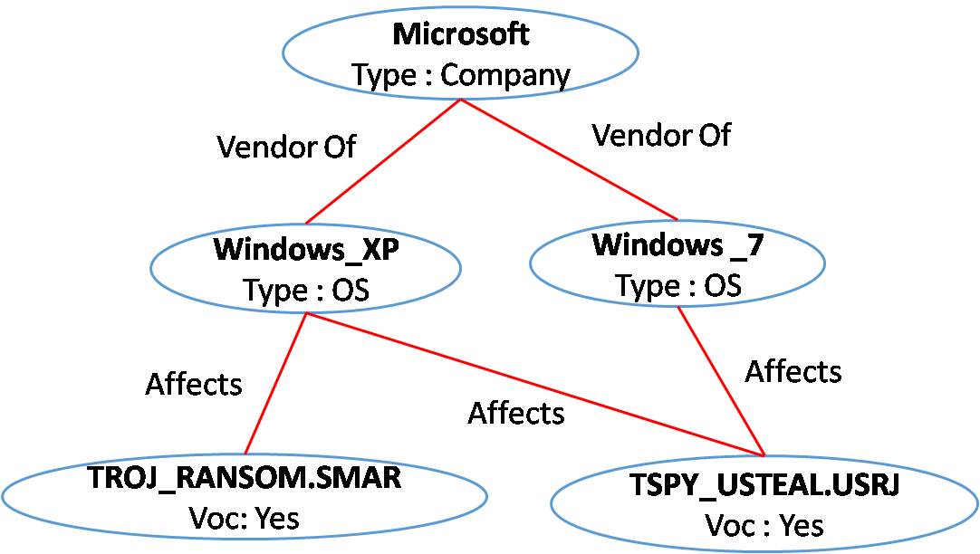
In the knowledge graph shown in Figure 3, we encode four types of information (1) domain vocabulary which indicates whether a concept is in the domain or not. In this example, we assume only the malware names are in the domain vocabulary (2) semantic category which encodes the properties or metadata associated with a concept (e.g., the type of Microsoft is a Company (3) Direct Relations which encode direct relations between two concepts (e.g., ”Microsoft” is a ”vendor of” ”Windows_XP”). (3) Indirect Relations which encode the relations among those who share a common node in the knowledge graph. For example, Windows_7 and Windows_XP are connected by a common intermediate node ”Microsoft”.
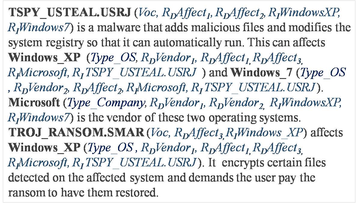
To convert the graph in Figure 3 into text annotations, first we need to rewrite this knowledge graph into predicate-argument structures . Here each predicate Pred represents a common property or relationship shared among all the arguments. With this representation, we want to indicate that all the arguments of the same predicate should be close to each other in the word embedding space since they either share a common property or are related by a direct or indirect relation. With this predicate-argument representation, we can easily translate them into text annotations. For example, the predicates will be translated to an annotation of each argument. Table 1 shows the predicate-argument structures that encode the knowledge graph in Figure 3. Finally, Figure 4 shows the text annotated with the information in the predicate-argument structures.
| Domain Vocabulary |
|---|
| Voc(TROJ_RANSOM.SMAR, TSPY_USTEAL.USRJ) |
| Semantic Category |
| TYPE_OS(Windows_XP, Windows_7) |
| TYPE_Company(Microsoft) |
| Direct Relation |
| =(Microsoft, Windows_XP) |
| =(Microsoft, Windows_7) |
| =(TSPY_USTEAL.USRJ, Windows_XP) |
| =(TSPY_USTEAL.USRJ, Windows_7) |
| =(TROJ_RANSOM.SMAR, Windows_XP) |
| Indirect Relation |
| =(Windows_XP, Windows_7) |
| =(Microsoft, TROJ_RANSOM.SMAR, TSPY_USTEAL.USRJ) |
| =(Microsoft, TSPY_USTEAL.USRJ) |
| =(Windows_XP, Windows_7) |
In general, the nodes represented in a knowledge graph are concepts. We need to map a concept of words or terms in the text in order to generate text annotations. Since in principle, the concept of word mapping is a one to many relation, it is possible that the same concept can be expressed by different words or phrases. For example, there are multiple ways to refer to the company ”IBM” in text such as ”International Business Machines”, ”IBM” or ”Big Blue”. Since currently, we have only implemented a simple 1 to 1 mapping, we need to explicit enumerate different surface expressions in multiple predicate-argument structures. For example, to indicate that IBM is the vendor of DB2, we need to produce three predicate-argument structures: (IBM, DB2), (International_Business _Machines, DB2), (Big_Blue, DB2). In out system, Multi-word terms are concatenated into a single token during a pre-processing step.
Annotation and Word Embedding (AWE)
We propose a novel AWE algorithm to learn word embeddings with text annotations. The inputs to our system are texts as well as annotations. If no annotations are available, our system is the same as a classic Word2Vec system. The output of our model includes not only a vector representation of each word but also a vector representation of each annotation in the same embedding space. For example, if Type_Trojan is an annotation in our dataset, the algorithm will also learn a vector representation for Tpye_Trojan based on the context of all the Trojan malware. We have implemented two AWE architectures.
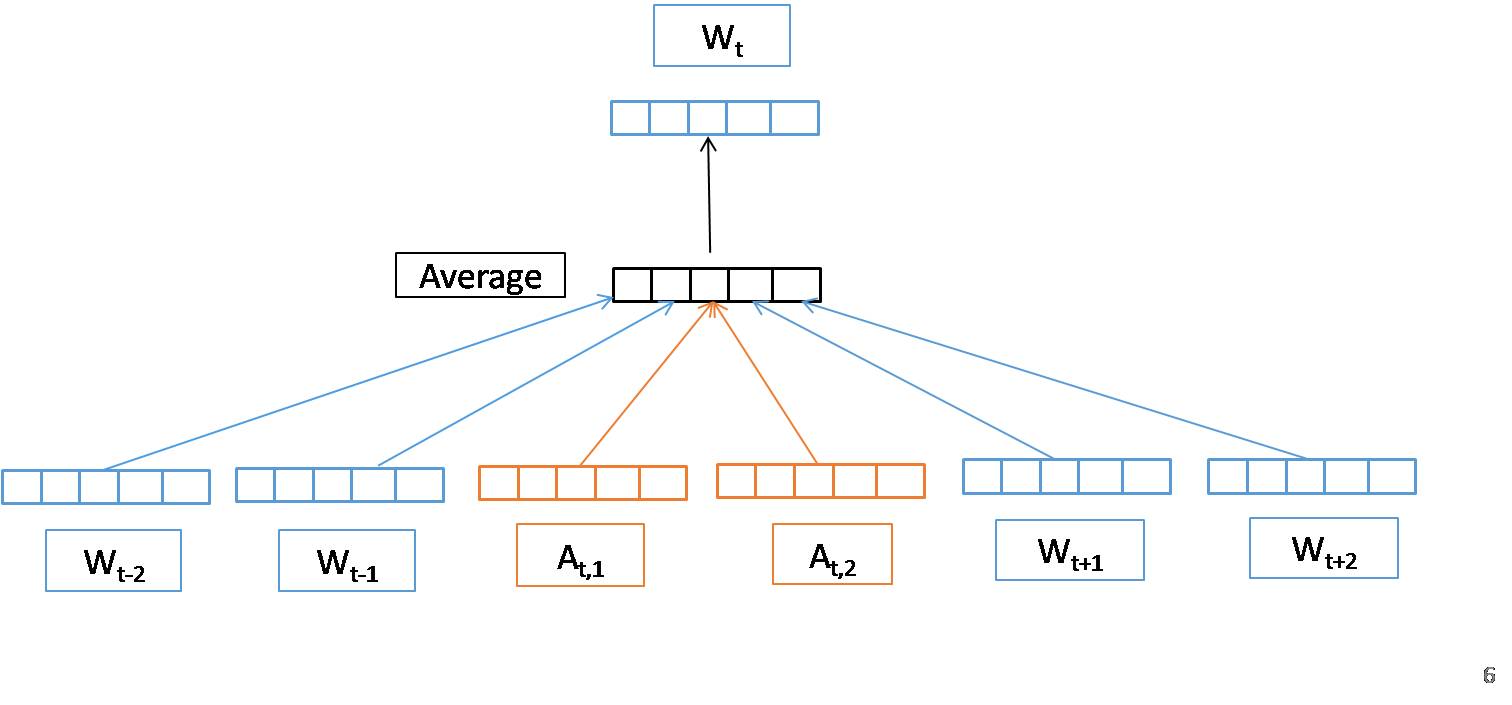
Annotation-Assisted Word Prediction (AAWP) With the AAWP architecture shown in Figure 5, the learning task is to predict a word given its annotations plus the other words in its context. A sliding window on the input text stream is employed to generate the training samples. In each sliding window, the model tries to use the surrounding words plus the annotations of the target word as the input to predict the target word. More formally, assume a word has a set of annotations (, , … ). Given a sequence of training words , … , … , the objective of the AAWP model is to maximize the average log probability shown in Equation 1
| (1) |
Where is the size of the context window, is the target word, is a context word, is the annotation of target word .
After training, every word is mapped to a unique vector, represented by a column in a weight matrix . The column is indexed by the position of a word in the vocabulary. Every annotation is also mapped to a unique vector, represented by a column in a weight matrix . The average of the vectors of the context words and the vectors of the annotations of the target word are then used as features to predict the target word in a context window. The prediction is done via a hierarchical softmax classifier. The structure of the hierarchical softmax is a binary Huffman tree where short codes are assigned to frequent words. The model is trained using stochastic gradient descent where the gradient is obtained via backpropagation. After the training process converges, the weight matrix is regarded as the learned word representations and as learned annotation representations.
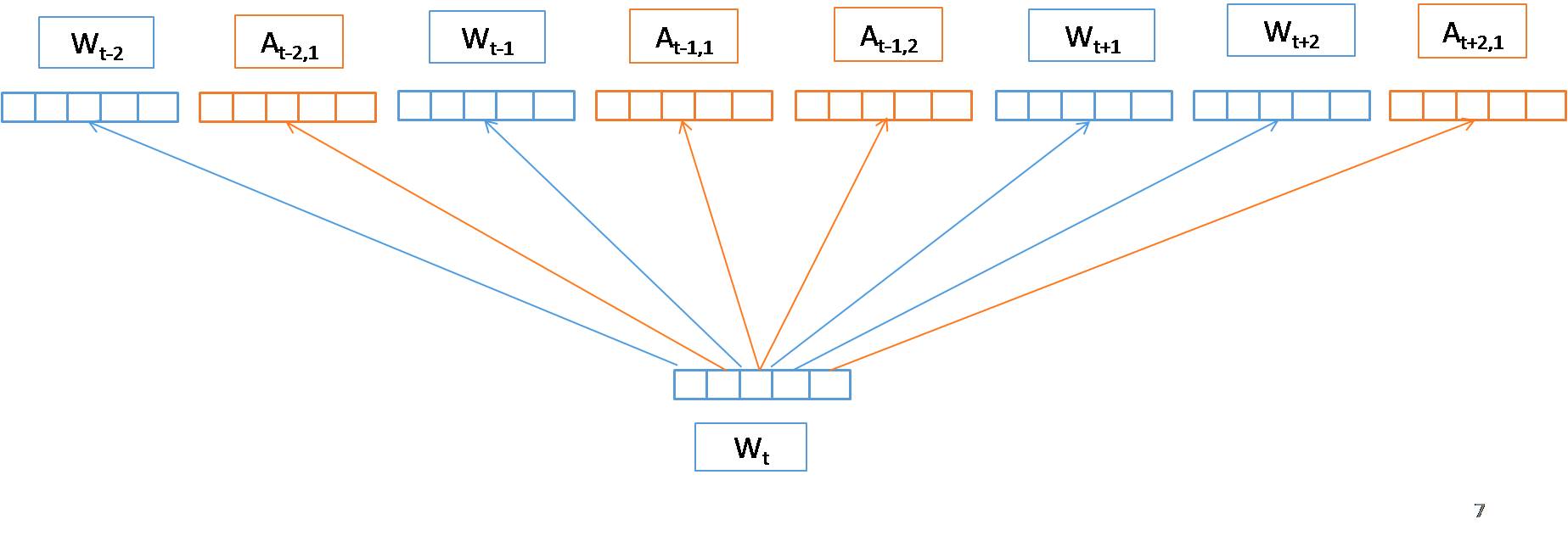
Joint Word and Annotation Prediction (JWAP) With the JWAP architecture shown in Figure 6, the task is to predict the context words and their annotations based on a target word. A sliding window is employed on the input text stream to generate the training samples. In each sliding window, in addition to predicting the context words, as in typical word embedding models, if the context words have one or more annotations, then the vector of the target word will also be used to predict the vectors of those annotations.
More formally, given a sequence of training words (, … , …) and their annotations ((, the objective of the JWAP model is to maximize the average log probability shown in Equation 2.
| (2) |
Where is the size of the context window, is the target word, is a context word, is the annotation of the context word , and is the number of annotations associated with the context word . The prediction is also done via hierarchical softmax. After the training process converges, the weight matrix is regarded as the learned word representations and as learned annotation representations.
Evaluation
In this section, we describe the experiments we conducted to examine the effectiveness of the proposed method. In particular, we compare the performance of our method with that of multiple state-of-the-art baselines. In the rest of this section, we first introduce each of the baseline models used in the evaluation, followed by a description of the evaluation methods and the results.
Baseline Models
The baseline models we used includes Word2Vec (?), a state of the art general-purpose word embedding system, Doc2Vec (?), a variable length sentence embedding system, Dis2Vec (?), a domain-specific word embedding method designed to incorporate disease-related domain vocabulary in word embeddings and a retrofitting model to incorporate semantic relations (?).
Word2Vec: This is one of the most widely adopted general-purpose word embedding tools. In our experiments, we have tested different Word2Vec models with different training methods. For example, there are two separate Word2Vec models, the CBOW model and the Skip-Gram model. The CBOW model tries to maximize the log likelihood of a target word given its context words. In contrast, the Skip-Gram model tries to maximize the log likelihood of the context words in a sliding window given a target word. In addition, different training methods may have significant impact on their performance. For example, it has been shown that Word2Vec trained with hierarchical softmax often performed better on sparse datasets than that trained with negative sampling (?). In total, we have tested four Word2Vec models: CBOW trained with hierarchical softmax, CBOW with negative sampling, Skip-Gram with hierarchical softmax and Skip-Gram with negative sampling.
Doc2Vec: Since each malware and CVE name is associated with a text description, it is possible to represent the meaning of a malware or CVE by aggregating the meaning of all the words in the description. We have chosen Doc2Vec to learn a vector representation of the malware (or CVE) description. Doc2Vec is a popular unsupervised neural network-based embedding method that learns fixed-length feature representations from variable-length texts, such as sentences, paragraphs, and documents. In Doc2Vec every document is mapped to a document vector and every word is mapped to a word vector. Doc2Vec also employs two different architectures: Distributed Memory (DM) and Distributed Bag of Words (DBOW). In DM, the document vector and vectors of the context words in a sliding window are aggregated together to predict the target word. In DBOW, the document vector is used to predict the words randomly sampled from the document.
Dis2Vec: It tries to incorporate disease-related vocabulary to improve the quality of domain-specific word embeddings. Each word pair is classified into three categories:
-
1.
-
2.
-
3.
.
Depending on which category a word and its context word belong to, different objective functions are used. For example, when both the target and the context word are from the domain vocabulary, the objective function shown in Equation 3 is used. The goal is to derive similar embeddings for them by maximizing the dot product of the two vectors.
| (3) |
Here being the uniform distribution on the interval is a smoothing parameter and is a sampling parameter, is a negative context, is the collection of (w, c) pairs for which is the collection of (w, c) pairs for which .
For a word pair from the second category where neither the target nor the context word is from the domain vocabulary, the classic Word2Vec objective function is used (as shown in Equation 4).
| (4) |
Finally, for word pairs from the third category where either the target word or the context word appears in the domain vocabulary but not both, the objective function shown in Equation 5 is used. The goal is to minimize the dot product of the vectors to generate dissimilar word vectors.
| (5) |
Where being the uniform distribution on the interval is soothing parameter and is objective selection parameter.
Retrofitting Word Vectors to Semantic Relations: This model refines existing word embeddings using semantic relations (?). This graph-based learning technique is applied as a post-processing step. Intuitively, this method encourages the new vectors to be similar to the vectors of related words as well as to their purely distributional representations.
Let = , . . . , be a vocabulary and Ω be an ontology that encodes semantic relations between words in the vocabulary . Let be an undirected graph (V, E) with one vertex for each word type and edges ( , ) E x indicating a semantic relationship. Let the matrix be the collection of original vector representations for each learned using any word embedding technique, where is the length of the word vectors. The objective is to learn the matrix Q = (,…) such that the columns are close to both their counterparts in and adjacent vertices in . Equation 6 shows the objective function:
| (6) |
Where and control the relative strengths of the associations.
Experiments
To train our AWE models, we need a text corpus plus some additional domain knowledge. Since our cybersecurity datasets include additional metadata, in our experiments, we focus on incorporating domain metadata in word embedding. For the malware dataset, we incorporate malware type and systems infected444we mapped threat type and platform in Trend Micro to malware type and systems affected in Symantec since they are roughly the same. For the CVE dataset, we incorporate vendor and product. All the metadata that is available to our system is also available to all the baselines as either metadata or text (some baselines can only take text as input). After we create our annotations, we train two AWE models: AAWP and JWAP. We have experimented with different embedding vector and context window sizes and our system works the best with embedding dimension size of 100 and context window size of 5.
To evaluate the quality of the learned embeddings by different methods, people often use the cosine similarity of the embeddings of many word pairs and its correlation (Spearman or Pearson) with human-assessed relatedness scores (?) However, this would require word pairs with a diverse set of similarity scores as the ground truth, which can be difficult to obtain since only experts with deep domain knowledge capable of creating such a ground truth for cybersecurity texts. Instead, we rely on the ground truth that can be generated directly from existing data sources. Specifically, for the malware dataset, we focus on pairs of malware names that were identified as aliases by either Symantec or Trend Micro. A total of 69 pairs of malware names were cross-referenced as aliases by at least one of the companies. For instance, TROJ_PSINJECT.A from Trend Micro specifies Symantec’s Trojan.Malscript as an alias. For the CVE dataset, we created pairs of related CVE names based on whether they belong to the same CVE family and also exploit the vulnerability of the same product. A total of 54 pairs of relevant CVEs were included in our CVE test data.
To evaluate the quality of word embeddings based on semantically equivalent or related word pairs (e.g., malware aliases or relevant CVEs), we can either use the mean cosine similarity of their embeddings (?) or the Mean Reciprocal Rank (MRR) (?). Since our focus is not to increase the absolute similarity score of the word pairs but to improve the rank of our target malware/CVE so that we can find them first in a list of most similar malware/CVEs. For example, Dis2Vec, one of the baseline models that incorporates domain vocabulary in word embedding, brings all the in-domain words close to each other while separating the in-domain words from out-domain ones. If a simple cosine similarity based measure is used, Dis2Vec would be considered effective since it increases the average similarity between the word pairs in our test dataset. Since all the malware or CVE names are in the cybersecurity vocabulary, Dis2Vec brings all of them close to each other, which will not help us find the equivalent or most relevant malware/CVE first.
Equation 7 shows the formula for computing MRR, where =(,,….) is a set of malware ( or CVEs) in our domain. =( and ) is the pair in a total of evaluation pairs. is the embedding vector for , is a set that includes all the embedding vectors excluding . The function cos produces a vector of cosine similarity scores, each is the cosine similarity of and one the domain embedding vectors excluding . The function returns the rank of among all the elements of .
| (7) |
Evaluation Results
We have tested all the embedding models on both datasets. Table 2 shows the results on the malware dataset.
| Model | MRR |
|---|---|
| CBOW with negative sampling | 50% |
| CBOW with hierarchical softmax | 44% |
| Skip-gram with negative sampling | 48% |
| Skip-gram with hierarchical softmax | 28% |
| Doc2Vec (DM) | 30% |
| Doc2Vec (DBOW) | 44% |
| Dis2vec | 58% |
| Retrofitting | 28% |
| AAWP (new) | 41% |
| JAWP (new) | 12% |
From the result, we can see that the JWAP model out-performed all the other models with the highest MRR of 12%, which represents a 57.14% MRR improvement over the next best models, the Retrofitting model and the Skip Gram model with hierarchical softmax. In addition, among the two AWE model we proposed, the JWAP is more effective than AAWP. Here JWAP uses the target word to predict the words and annotations in its context while the AAWP model relies on the context words as well as the annotations of the target word to predict the target word. In fact, the AAWP model is a generalization of the CBOW model while the JWAP model is a generalization of the Skip-Gram model. Previously, it was also shown that the Skip-Gram model often outperformed the CBOW model in generating general purpose word embeddings (?). In addition, hierarchical softmax works better than models trained with Negative Sampling. This is also quite consistent with previous findings. Previously, it was shown that Negative Sampling often generates better word embeddings for frequent words while hierarchical softmax works better for rare words. Since each malware/CVE name in our dataset occurs only once or twice, hierarchical softmax is more effective than negative sampling in identifying semantic relations between rare words. Under the MRR measure, the vocabulary based Dis2Vec failed to improve over the general domain word embedding models. Moreover, using document embedding to represent a domain concept (e.g., malware and CVE) does not seem to be very effective.
Table 3 shows the evaluation results on the CVE dataset.
| Model | MRR |
|---|---|
| CBOW negative sampling | 43% |
| CBOW hierarchical softmax | 29% |
| Skip-gram negative sampling | 41% |
| Skip-gram hierarchical softmax | 9% |
| Doc2Vec (DM) | 33% |
| Doc2Vec (DBOW) | 37 % |
| Dis2vec Model | 26% |
| Retrofitting Model | 9% |
| AAWP Model (new) | 29% |
| JWAP model (new) | 7% |
The result on the CVE dataset is very similar to those on the malware dataset. Again, the JWAP model out-performed all the other models with the highest MRR of 7%, which represents a 22.22% MRR improvement over the next best systems, the retrofitting model and the Skip- Gram with hierarchical softmax model. Among the two new models we proposed, JWAP also performed significantly better than AAWP. Again, the document embedding models and the Dis2Vec did not perform well. The document vocabulary did not provide useful information to support our evaluation tasks.
Discussion
The effectiveness of our model largely depends on the quality of the annotations. If annotations are inconsistent then our model won’t be able to generate good embeddings. For example, in our malware dataset, we used malware type to generate annotations. But malware types defined by different companies are inconsistent. For example TSPY_SHIZ.MJSU and INFOSTEALER.SHIZ are the names of the same malware. In the Trend Micro dataset, it is categorized as a spyware while in the Symantec dataset, it is categorized as a Trojan. overall, trojans and worms are two malware types that are most inconsistent across different companies. Since our model tries to generate similar word embeddings for words with the same annotations, inconsistent metadata will prevent the system from achieving this.
Conclusion
In this paper, we present a novel word embedding model for sparse domain texts. To overcome the sparsity, we incorporate diverse types of domain knowledge which is available in many domains. We propose a text annotation-based framework to represent diverse types of domain knowledge such as domain vocabulary, semantic categories, semantic relations and other metadata. We have also developed a novel Word and Annotation Embedding (AWE) method which is capable of incorporating annotations in word embedding. We have evaluated the effectiveness of our algorithm using two cybersecurity corpora: the malware dataset and the CVE dataset. We describe a series of experiments to compare our method with existing word embedding methods developed for both general and specific domains. Our results demonstrate that our model outperformed the next best model by a significant margin. The improvement over the best baseline model is 22% to 57% MRR reduction. The learned word embeddings can be a useful resource to support many downstream domain-specific NLP tasks. Currently, we are applying learned word embeddings to support Information Extraction for cybersecurity texts.
References
- [Bansal, Gimpel, and Livescu 2014] Bansal, M.; Gimpel, K.; and Livescu, K. 2014. Tailoring continuous word representations for dependency parsing. In ACL (2), 809–815.
- [Bengio et al. 2003] Bengio, Y.; Ducharme, R.; Vincent, P.; and Jauvin, C. 2003. A neural probabilistic language model. Journal of machine learning research 3(Feb):1137–1155.
- [Bian, Gao, and Liu 2014] Bian, J.; Gao, B.; and Liu, T.-Y. 2014. Knowledge-powered deep learning for word embedding. In Joint European Conference on Machine Learning and Knowledge Discovery in Databases, 132–148. Springer.
- [Bollegala et al. 2016] Bollegala, D.; Alsuhaibani, M.; Maehara, T.; and Kawarabayashi, K.-i. 2016. Joint word representation learning using a corpus and a semantic lexicon. In AAAI, 2690–2696.
- [Collobert and Weston 2008] Collobert, R., and Weston, J. 2008. A unified architecture for natural language processing: Deep neural networks with multitask learning. In Proceedings of the 25th international conference on Machine learning, 160–167. ACM.
- [Faruqui et al. 2014] Faruqui, M.; Dodge, J.; Jauhar, S. K.; Dyer, C.; Hovy, E.; and Smith, N. A. 2014. Retrofitting word vectors to semantic lexicons. arXiv preprint arXiv:1411.4166.
- [Fu et al. 2014] Fu, R.; Guo, J.; Qin, B.; Che, W.; Wang, H.; and Liu, T. 2014. Learning semantic hierarchies via word embeddings. In ACL (1), 1199–1209.
- [Ghosh et al. 2016] Ghosh, S.; Chakraborty, P.; Cohn, E.; Brownstein, J. S.; and Ramakrishnan, N. 2016. Designing domain specific word embeddings: Applications to disease surveillance. arXiv preprint arXiv:1603.00106.
- [Lample et al. 2016] Lample, G.; Ballesteros, M.; Subramanian, S.; Kawakami, K.; and Dyer, C. 2016. Neural architectures for named entity recognition. arXiv preprint arXiv:1603.01360.
- [Le and Mikolov 2014] Le, Q., and Mikolov, T. 2014. Distributed representations of sentences and documents. In Proceedings of the 31st International Conference on Machine Learning (ICML-14), 1188–1196.
- [LeCun, Bengio, and Hinton 2015] LeCun, Y.; Bengio, Y.; and Hinton, G. 2015. Deep learning. Nature 521(7553):436–444.
- [Levy and Goldberg 2014] Levy, O., and Goldberg, Y. 2014. Dependency-based word embeddings. In ACL (2), 302–308.
- [Luong, Socher, and Manning 2013] Luong, T.; Socher, R.; and Manning, C. D. 2013. Better word representations with recursive neural networks for morphology. In CoNLL, 104–113.
- [Maas et al. 2011] Maas, A. L.; Daly, R. E.; Pham, P. T.; Huang, D.; Ng, A. Y.; and Potts, C. 2011. Learning word vectors for sentiment analysis. In Proceedings of the 49th Annual Meeting of the Association for Computational Linguistics: Human Language Technologies-Volume 1, 142–150. Association for Computational Linguistics.
- [Mikolov et al. 2011] Mikolov, T.; Kombrink, S.; Burget, L.; Černockỳ, J.; and Khudanpur, S. 2011. Extensions of recurrent neural network language model. In Acoustics, Speech and Signal Processing (ICASSP), 2011 IEEE International Conference on, 5528–5531. IEEE.
- [Mikolov et al. 2013a] Mikolov, T.; Chen, K.; Corrado, G.; and Dean, J. 2013a. Efficient estimation of word representations in vector space. arXiv preprint arXiv:1301.3781.
- [Mikolov et al. 2013b] Mikolov, T.; Sutskever, I.; Chen, K.; Corrado, G. S.; and Dean, J. 2013b. Distributed representations of words and phrases and their compositionality. In Advances in neural information processing systems, 3111–3119.
- [Mnih and Hinton 2009] Mnih, A., and Hinton, G. E. 2009. A scalable hierarchical distributed language model. In Advances in neural information processing systems, 1081–1088.
- [Nguyen and Grishman 2015] Nguyen, T. H., and Grishman, R. 2015. Relation extraction: Perspective from convolutional neural networks. In VS@ HLT-NAACL, 39–48.
- [Pennington, Socher, and Manning 2014] Pennington, J.; Socher, R.; and Manning, C. 2014. Glove: Global vectors for word representation. In Proceedings of the 2014 conference on empirical methods in natural language processing (EMNLP), 1532–1543.
- [Santos and Guimaraes 2015] Santos, C. N. d., and Guimaraes, V. 2015. Boosting named entity recognition with neural character embeddings. arXiv preprint arXiv:1505.05008.
- [Schnabel et al. 2015] Schnabel, T.; Labutov, I.; Mimno, D. M.; and Joachims, T. 2015. Evaluation methods for unsupervised word embeddings. In EMNLP, 298–307.
- [Tang et al. 2014] Tang, D.; Wei, F.; Yang, N.; Zhou, M.; Liu, T.; and Qin, B. 2014. Learning sentiment-specific word embedding for twitter sentiment classification. In ACL (1), 1555–1565.
- [Voorhees and others 1999] Voorhees, E. M., et al. 1999. The trec-8 question answering track report. In Trec, volume 99, 77–82.
- [Xu et al. 2014] Xu, C.; Bai, Y.; Bian, J.; Gao, B.; Wang, G.; Liu, X.; and Liu, T.-Y. 2014. Rc-net: A general framework for incorporating knowledge into word representations. In Proceedings of the 23rd ACM International Conference on Conference on Information and Knowledge Management, 1219–1228. ACM.
- [Yu and Dredze 2014] Yu, M., and Dredze, M. 2014. Improving lexical embeddings with semantic knowledge. In ACL (2), 545–550.