Metref et al.Model evidence using data assimilation with localization
Sammy Metref, IFAECI, CNRS-CONICET-UBA, Pab. II, piso 2, Ciudad Universitaria 1428 Buenos Aires, Argentina, Tel.: +5411-4787-2693, Fax: +5411-4788-3572, e-mail: sammy.metref@cima.fcen.uba.ar
Estimating model evidence using ensemble-based data assimilation with localization - The model selection problem
Abstract
In recent years, there has been a growing interest in applying data assimilation (DA) methods, originally designed for state estimation, to the model selection problem. In this setting, Carrassi et al. (2017) introduced the contextual formulation of model evidence (CME) and showed that CME can be efficiently computed using a hierarchy of ensemble-based DA procedures. Although Carrassi et al. (2017) analyzed the DA methods most commonly used for operational atmospheric and oceanic prediction worldwide, they did not study these methods in conjunction with localization to a specific domain. Yet any application of ensemble DA methods to realistic geophysical models requires the implementation of some form of localization. The present study extends the theory for estimating CME to ensemble DA methods with domain localization. The domain-localized CME (DL-CME) developed herein is tested for model selection with two models: (i) the Lorenz 40-variable mid-latitude atmospheric dynamics model (L95); and (ii) the simplified global atmospheric SPEEDY model. The CME is compared to the root-mean-square-error (RMSE) as a metric for model selection. The experiments show that CME improves systematically over the RMSE, and that this skill improvement is further enhanced by applying localization in the estimate of the CME, using the DL-CME. The potential use and range of applications of the CME and DL-CME as a model selection metric are also discussed.
keywords:
Contextual model evidence; Ensemble Kalman Filter; Localization; Parameter estimation; Detection and attribution1 Introduction and motivations
Model selection in the broader literature is the task of selecting a statistical model from a set of candidate models, given data (e.g., Ando, 2010). More precisely (Baum et al., 1970), it is the problem of defining and using metrics to compare different models or different model versions, i.e., different versions of the same model that may differ by the model’s parameters, its subgrid-scale parameterisations or its boundary conditions.
Either model selection or, more specifically, systematic model version selection, though, have received little attention from the geoscientific community, as compared to data assimilation (DA), which is by now a well-established field in the geosciences (Daley, 1991; Ghil and Malanotte-Rizzoli, 1991; Bennett, 1992; Kalnay, 2003; Asch et al., 2016; Carrassi et al., 2018). DA, though, has focused so far mainly on estimating high-dimensional states of the atmosphere (Whitaker et al., 2008; Buehner et al., 2010), of the ocean (Lermusiaux, 2006; Sakov et al., 2012) and of the climate system as a whole (Saha et al., 2010; Saha et al., 2014). Even nowadays, common practice in evaluating models and successive versions thereof at operational centers is to compare visually model outputs to observations or, more quantitatively, to compute the model-to-data root-mean-square error (RMSE).
Some attempts to analytically address the model or model version selection problem have been successful (e.g., Winiarek et al., 2011) but only under specific assumptions that may not be realistic for large-dimensional geoscientific applications. Numerical methodologies that may be computationally affordable for high-dimensional problems have also been proposed in recent years (Särkkä, 2013; Elsheikh et al., 2014a, b; Otsuka and Miyoshi, 2015; Reich and Cotter, 2015; Carson et al., 2017; Carrassi et al., 2017). Several of these approaches advocate the use of the marginal likelihood of the data — also called model evidence — for model selection. Along these lines, the contextual formulation of model evidence (CME), first proposed by Hannart et al. (2016b) and fleshed out by Carrassi et al. (2017), exploits DA techniques to approach the model selection problem.
Carrassi et al. (2017) provide the analytic formulae to compute the CME using several state-of-the-art Gaussian ensemble DA methods and demonstrate the benefits of CME as a model selecting tool. Their study thus started to answer the first theoretical and practical research questions that had to be addressed to make the CME suitable for model version selection operationally in weather forecasting centers.
Nevertheless, a number of issues remain to be tackled in order to proceed to the operational implementation of the CME. Among these, one key issue is the use of spatial localization — simply called henceforth localization — in ensemble-based DA. Indeed, when applied to large-dimensional models, the ensemble based DA methods of Carrassi et al. (2017) to compute CME would fail unless localization is properly incorporated. Even though localization is a widely established practice in ensemble DA, and has also generated a substantial literature (e.g., Houtekamer and Mitchell, 2001; Hamill et al., 2001; Ott et al., 2004 and Sakov and Bertino, 2011), it is still a topic of very active research.
Localization originally arose as a countermeasure to the sampling issue due to our attempt to describe uncertainty in high dimensions using a very limited ensemble. Help in overcoming this problem comes from the fact that many physical systems, and notably the atmosphere and ocean, tend to have small long-distance correlations, i.e., the actual error covariances are sparse (e.g., Ghil et al., 1979; Balgovind et al., 1983). For such systems, localization can – without degrading too severely a physical system’s representation – set long-distance correlations to zero and only model the terms in the covariance matrix that are close to the diagonal.
Many localization techniques exist to achieve sufficiently accurate approximations of the covariance matrix along these lines. These techniques, though, do lead to a change in the structure of the matrices manipulated during the DA process. Hence, in the CME context, the challenge is to adapt its original formulation to the need for localization in the underlying DA process. This study aims, therefore, to extend CME theory, as presented in Carrassi et al. (2017), to include localization and to apply it to a quasi-realistic atmospheric model of intermediate complexity.
The structure of the paper is as follow. Section 2 recalls the benefits of approaching model evidence using the DA framework. A more extensive discussion of these benefits can be found in Hannart et al. (2016b). Section 3 first introduces the notion of localization in general, and the domain localization technique in particular. The application of domain localization in the CME computation is hereafter referred to as the domain-localized CME (DL-CME), and it is also presented in section 3. Section 4 implements the two CME formulations, with and without localization, and compares them to the RMSE as indicators of model version selection in various numerical experiments based on the 40-dimensional L95 model of Lorenz (1996). Section 5 applies these indicators to a parameter selection problem using the simplified global atmospheric model called SPEEDY (Molteni, 2003; Kucharski, 2006). Section 6 finally provides a summary, conclusions and future directions.
2 Model evidence and data assimilation
Let us assume that a model describes an unknown process at time , as a -dimensional state , that we only perceive via a set of partial, -dimensional observations .
The model .
The model simulates the unknown process
| (1) |
where propagates the state from time to time . The dimension of the model state can be decomposed as , where is the space of the physical variables, such as temperature and velocity components, while is the set of finite modes of the model that represent the physical variables.
In general, is the model error — represented most often by an additive stochastic white noise — but here we shall assume that the model is perfect, i.e., . The implications of this assumption on the computation of the CME are substantial, cf. Carrassi et al. (2017), but we have reason to believe that it does not affect very much our conclusions about the impact of localization on the CME and its comparison with the RMSE. . This perfect model assumption will be removed in subsequent studies.
The set of observations y.
The observation vector is related to the state vector according to the observation model
| (2) |
Here is the observational operator at time and is the observation error, represented here as an additive stochastic white noise with zero mean and covariance , which is assumed to be constant in time.
2.1 CME for model version selection
Using a given model of type and the set of observations , the goal of model version selection is to define a metric based on them, and apply it to identify the best model. Several metrics for model version selection are defined in the literature (Akaike, 1974; Schwarz, 1978; Burnham and Anderson, 2002). In the present article, we focus on model evidence as the metric of choice (Särkkä, 2013; Elsheikh et al., 2014a, b; Otsuka and Miyoshi, 2015; Reich and Cotter, 2015; Carson et al., 2017; Carrassi et al., 2017).
2.1.1 Model evidence
Let us define the ideal infinite set of observations as . The marginal likelihood of , given , is calculated as
| (3) |
This likelihood is also referred to as model evidence.
Note that, in the context of model evaluation, one should rather be interested in estimating the probability of the model conditioned on the observations . Yet, model evidence can be used to construct a metric either for model version selection or for the comparison between two distinct models and .
To see this, let us write the ratio of the two posterior distributions, each one relative to models and respectively, conditioned on the same set of observations
| (4) |
Equation (4) computes the ratio of the posterior model probability density functions (pdfs) and we see that it is proportional to the ratio of the model evidences – the Bayesian factor – times the ratio of the prior model pdfs. The latter are difficult to evaluate in practice, but, it is often legitimate to assume that the prior pdfs of the two models are the same, provided that we do not possess enough information to favor one model over the other. In this case, we see how the Bayesian factor provides an estimate of the model pdf ratio. In any case, the Bayesian factor is the scalar that updates the ratio of prior model pdfs to the ratio of posterior model pdfs.
In this sense, the ratio of the two model evidences can be considered as a selection indicator that favors one model or the other, depending on . More conveniently, one can look at the difference between their respective logarithms, and write the model selection indicator as
| (5) |
We use the indicator in the following experiments, and the model selection criterion becomes .
2.1.2 Contextual model evidence (CME)
If the model is autonomous, one can condition model evidence on the initial observation of the set, and write
| (6) |
where the explicit dependence on has been dropped on the right-hand side for the sake of clarity, and where is the likelihood of the observations from time to conditioned on all observations up to and including time .
A significant difference between the CME method employed here and previous methods (Särkkä, 2013; Reich and Cotter, 2015; Del Moral, 2004) is the use of the current-time density as a prior. This choice allows one to narrow the probability density so as to focus on plausible states given the current conditions of a system. The latter are embedded in our, inevitably approximate, knowledge of the prior. Indeed, an alternative formulation of the model evidence, which also can give a computational gain, is to no longer try to estimate the climatological model evidence – which is difficult to estimate accurately and which does not provide information on the present context of the system – but the so called contextual model evidence (CME), (Carrassi et al., 2017). This new contextual view of model evidence implicitly assumes that all information from past observations is conveyed by conditioning on .
Marginalizing over yields
| (7) |
Therefore, the two terms needed to compute the CME are:
-
•
the conditional pdf, , and
-
•
the likelihood of the observations, .
The conditional pdf is the posterior pdf, or analysis, produced by the state estimation DA process. The observational likelihood is often a given quantity (or at least considered as such) of the state estimation DA problem. Hence, as shown in Carrassi et al. (2017), the CME can be obtained as a by-product of a DA algorithm designed to assimilate the data y into the model .
2.2 The CME’s EnKF-formulation
We present here the CME formulation based on the ensemble Kalman filter (EnKF: Evensen, 2009). The choice of the EnKF among other, possibly even more accurate, methods to compute CME, is motivated by its great cost/benefit ratio. Carrassi et al. (2017) showed that the CME evaluated by the EnKF achieves high accuracy and discrimination skills – that is only slightly lower than when evaluated by other more sophisticated DA methods – but does so at a much lower computational cost. In fact, Carrassi et al. (2017) also showed that – although the DA schemes with the coarsest approximations (e.g., the EnKF) provide the worst estimates of the CME in a strongly nonlinear system, such as the Lorenz (1963) model – the performance of these schemes in estimating the CME is comparable, regardless of their respective approximations, in a weakly nonlinear system like the L95 model. Hence, in atmospheric, oceanic or coupled systems at synoptic scales, which behave in a quasi-linear and quasi-Gaussian manner most of the time, the differences produced by the choice of assimilation scheme are expected to be negligible compared to the difference between two model versions.
The EnKF-formulation of the CME comes as a by-product of the EnKF DA process that gives an approximation of model evidence . Over the evidencing window , of size , the CME is calculated as
| (8) | ||||
where is the prior state estimate at time , and where , while is the prior error covariance matrix.
Note that, whilst the RMSE is the Euclidean distance between the first guess and the observations, the CME can be seen as a distance between the same two fields, ponderated by the matrix . Hence, the uncertainty on the prior and the uncertainty R on the data both penalize the CME. In other words, overfitting the model to the data, due to a faulty assimilation, will not erroneously decrease the CME. The CME will thus be able to spot and penalize a model-to-data overfit, whereas the RMSE that does not take into account the prior and the data uncertainties will not.
There are two different proofs of the EnKF-based CME in Eq. (8), one for the stochastic EnKF in Hannart et al. (2016b) and another for the deterministic EnKF in Carrassi et al. (2017): both are referred to hereafter as the global CME (G-CME).
An efficient alternative to compute the G-CME is presented in Alternative implementation of the global CME (G-CME) and it is used throughout the present article. This implementation assumes that R is diagonal, i.e., that the observations are mutually uncorrelated, an assumption that is often made in the geosciences and elsewhere. A significant improvement achieved by this alternative G-CME implementation is that the problem is no longer solved in the physical space of dimension but in the reduced ensemble space of dimension , with in most cases. This implementation thus reduced significantly the computational cost of the experiments in the present paper.
3 CME and domain localization
This section presents a new formulation of the CME with domain localization. We describe first, in section 3.1, how domain localization is implemented within the DA process, and then the domain-localized CME (DL-CME) in section 3.2.
3.1 Domain localization
3.1.1 The basic idea
Domain localization dates back to earlier forms of DA, like the successive correction method (Cressman, 1959; Ghil et al., 1979; Ghil and Malanotte-Rizzoli, 1991). A variant known as local analysis was then introduced by Houtekamer and Mitchell (2001) and by Ott et al. (2002, 2004). Here, we describe a different approach to local analysis due to Hunt et al. (2007) and applicable in the Ensemble Transform Kalman Filter (ETKF) of Bishop et al. (2001) framework. The Local ETKF (LETKF) method of Hunt et al. (2007) consists in updating separately, at each spatial gridpoint , all the physical variables , with , by assimilating only neighboring observations; see section 3.1.2.
The first step of local analysis consists of selecting the observations within a disk centered on the spatial gridpoint we wish to update; the radius of this disk is a predefined parameter , called the cut-off radius. This type of selection process is often called the box-car scheme, as opposed to schemes that gradually taper off the weights given to observations, from to . Note that in general the cut-off radius depends on the physical variable to be analyzed.
We denote the resulting reduced observation vector by , and its size by . It is then also necessary to restrict the observation error covariance matrix R to a local matrix that has smaller dimension. However, the analysis resulting after the first step alone may – when the observations are sparse, for instance (Szunyogh et al., 2008) – present abrupt discontinuities at the boundary of the observation disk and have, therefore, a deleterious side-effect, whose elimination or mitigation requires a second analysis step.
The second step in local analysis applies a localization function to the inverse matrix , called precision matrix, and it produces a smoother global update. The localization function is in fact the Schur product (Hunt et al., 2007) of by the diagonal localization matrix giving
| (9) |
where is equal to if and it decreases gradually to outside of the disk of radius , called the localization radius. Hence, the further an observation lies from , the more its observation error variance is increased and its impact on the local analysis is decreased.
3.1.2 The LETKF
The ensemble transform Kalman filter (ETKF: Bishop et al., 2001) is a deterministic EnKF performing the analysis in the ensemble space. The ETKF computes the updated ensemble , with the ensemble members, such that
| (10) |
Here and , and the analysis ensemble is given by a linear combination of the forecast ensemble mean and the forecast ensemble anomalies in . Finally, and is the identity matrix.
The domain localization applied to the ETKF gives the LETKF of Hunt et al. (2007). In the LETKF, a separate analysis is performed for each model variable attached to a gridpoint of the spatial grid and the resulting update affects each physical variable at . The DA is performed using localized observations, i.e., the observation precision matrix is .
3.2 Domain-localized CME
In order to formulate the CME with domain localization, we start with the general case of an observation subvector of generic nature. In section 3.2.1, the case of the trivial evidencing window is treated first. Second, we address the inconsistency that arises when and show how to remove it by using realistic approximations. In section 3.2.2, we derive from the general case a formulation of the local CME. Finally, in section 3.2.3, we propose a heuristic global model version selection indicator based on local CMEs, the DL-CME.
3.2.1 CME of an observation subvector
Let us consider first the problem of estimating the CME of , a subvector of the original observation vector . Such a subvector may be obtained either by selecting a subset of observation types or by a spatial localization or both. The corresponding CME is just a particular case of the original DA, i.e., of the DA for the complete observation vector, and can be obtained by directly applying Eq. (7) to the subvector . Indeed, if the evidencing window has length , the contextual evidence of becomes
| (11) |
Both pdfs in the integrand above are by-products of the original DA: is the original posterior pdf at time and the sub-sampled likelihood also stems from the original DA process. Using the EnKF formalism, one can compute the CME for this subvector using Eq. (8) which in this case leads to
| (12) | ||||
Here , where , and are the observation operator, its linearization and the observation error covariance matrix corresponding to the observation subvector, respectively. Note that are the forecast products of the original DA.
If the evidencing window is longer, , we decompose the contextual evidence – according to Carrassi et al. (2017) – as
| (13) | ||||
The factor in Eq. (13) corresponds to the case and it can be computed from the original DA process using Eq. (12). The sub-sampled likelihoods are also easily computable since the likelihood of the observation is usually given in a state-estimation process.
The pdf of the system’s state, conditional on the observation subvectors for , however, requires a dedicated DA of the observation subvectors. It seems desirable to estimate these exact pdfs but the forecast-assimilation process required to do so may — depending on the nature of the observation subvectors — involve an insufficiently observed system and the DA algorithm may, therefore, fail to converge (cf. section 5.1.3).
In such a situation, approximating by the original posterior pdf, , is a possibility when the evidencing window is short enough. In this case, the EnKF-formulation can be used to compute the CME as
| (14) | ||||
where . Using instead of the above approximation the correct pdfs of the system’s state, conditional on the observation subvector , would require computing the ad-hoc in , instead of .
3.2.2 Local CME
In the same spirit as the local analysis above, we want to locally compute the CME at each spatial gridpoint . The reduced observation vectors can be considered as observation subvectors and we can use, therewith, the formalism of section 3.2.1.
Hence, for each spatial gridpoint , the local CME can be obtained from Eq. (14), yielding
| (15) | ||||
here ; and are, respectively, the restrictions of the nonlinear and the linearized observation operator to the neighborhood of . In other words, at the spatial point , the local CME returns the CME of the observations that have affected its analysis.
Analogously to the LETKF, this approach computes a local CME at each gridpoint. Another approach would be to taper directly the global matrix – as in the background covariance localization of Sec. 3.3 below. However, the high dimension of the systems we are interested in may not allow one to compute its inverse, . The local CME approach may seem costly but, in practice, the numerical gain of computing the CME on a small number of observations, within a local domain, overcomes the great number of local computations needed. Moreover, the local computation of the CME allows a full parallelization of the algorithm, which offers an important computational gain.
Note that, in the case of domain localization, it is not necessary to approximate the conditional pdf of the system’s state on the observation subvectors by the original posterior pdf, since is already the local approximation of . Nonetheless, the observation vectors represent a tube of observations spread in time over the evidencing window but confined to the same local domain. Due, however, to the physical evolution of the error covariances, such a static tube may not be as useful for DA and evidencing as would a dynamic tube that follows local domains and is covariant with the flow (Bocquet, 2016). Nevertheless, the implementation of such covariant localization techniques is not required for the short evidencing windows used here, so that we apply Eq. (15) without such corrections.
3.2.3 The DL-CME
Creating a global indicator from local CMEs is not theoretically straightforward. We propose instead a global heuristic indicator for model version selection , that we call the DL-CME,
| (16) |
here are positive, model grid–dependent coefficients, inversely proportional to the number of observations in the domain around , that weight the logarithms of the local CMEs, such that . For instance, in the L95 experiments of section 4, all the weights are set to be equal since the localization radius is constant throughout the domain. However, in the SPEEDY experiments (section 5), vary with the latitude as the number of gridpoints per local domain does.
3.3 Brief review of background covariance localization.
Another widely used technique for localization is the background covariance localization originally proposed by Houtekamer and Mitchell (2001). This localization consists in restricting the spatial impact of the unrealistic correlations due to the subsampling of the ensemble-based covariances, by directly applying a smoothing function onto the forecast error covariance matrix.
This technique can be applied to the computation of the CME in the same vein as DL-CME above, in order to take into account the actual covariances used by the DA. Details of the derivation of the CME formulation using background covariance localization are presented in Derivation of the CME formulation using background covariance localization. The computational cost remains the same as for the original EnKF-formulation plus the significant cost of a Schur product.
This alternative approach to CME localization can also be applied to large-dimensional systems, but only if combined with sophisticated numerical techniques to make it computationally feasible. For this reason, background covariance localization will not be discussed furthermore in the present article. Further studies investigating this matter should follow. See Carrassi et al., 2018 (their section 4.4) for a review on localization techinques in DA.
4 Numerical experiments with a toy model
The numerical experiments are designed to: (i) study numerically the performance of the global and local CME as a model version selection indicator and to compare it with the RMSE that is widely used for the same purposes; and (ii) analyze the impact of domain localization in the computation of the CME. These experiments use the L95 model (Lorenz, 1996; Lorenz and Emanuel, 1998).
4.1 Experimental setup
4.1.1 The Lorenz-95 (L95) model
The one-dimensional L95 model is a representation of atmospheric flow along a mid-latitude zonal circle with variables . In this case, and , i.e., one single physical variable, such as the stream function or the geopotential height, is defined at each grid point.
The model equations, according to Lorenz and Emanuel (1998), are the following
| (17) |
for and F represents the external forcing. The model integration is performed using a fourth-order Runge-Kutta scheme with a time step , in nondimensional units for which unity corresponds to 5 days (Lorenz, 1996).
In our model version selection problem, we consider the correct model version, given by Eq. (17) with . This value leads to chaotic behavior of the model, with a doubling time of errors equal to 2.1 days (Lorenz, 1996). We then generate various incorrect model versions, each of them with a different forcing term .
4.1.2 The DA implementation
A “true” trajectory is generated with the correct model version, in which . Observations are generated by sampling the true trajectory , every DA interval , using Eq. (2) with and , so that the full system is observed. The correct observation error covariance, , is used in the DA. The experiments are run over DA cycles, after a spin-up of DA cycles.
The DA method used throughout the present section is the LETKF described in section 3.1.2. The localization matrix, , is diagonal with coefficients defined by , where is the size of the reduced observation error covariance matrix, is the localization radius and is the Gaspari-Cohn function (Gaspari and Cohn, 1999) displayed in Eq. (30) of Derivation of the CME formulation using background covariance localization.
The performance of the DA algorithm is evaluated using the RMSE of the analysis with respect to the truth
| (18) |
with and being the true and the estimated state, respectively. Here and elsewhere we follow the superscript notation proposed by Ide et al. (1997) for the truth; the analysis, i.e. the estimated state; the forecast, i.e. the propagated state between consecutive observations, with ; and the observations.
The accuracy of the model version selection is assessed based on the RMSE of the forecast with respect to the observations
| (19) |
Model evidence, for both the G-CME and the DL-CME formulations, is evaluated over the evidencing window of size . Unless otherwise stated, we set here , which means that the model evidence is computed only for one DA cycle. This choice is made based on the fact that, in a selection problem, the smaller the evidencing window the more difficult it is to discriminate between two model versions (Carrassi et al., 2017). In practice, this means that the assimilation process is performed repeatedly in time and, at each available observation, the discrimination skills of the selection methods are assessed at the present time step, i.e., for the most difficult (i.e. least discriminating) selection problem, namely .
4.2 Numerical results
4.2.1 CME versus RMSE
In this subsection, we focus on the performance of the G-CME (Eq. 8) — i.e., without localization — as the model version selection indicator, and compare it with that of the RMSE.
For each model version, i.e. for each choice of the forcing F, a DA is performed using the setup described in section 4.1.2, with a 40-member ensemble (), without localization and with a coefficient of inflation tuned to provide the smallest RMSEt (Eq. 18) for each DA. At each cycle of the experiment, the G-CME and RMSE indicators are computed.
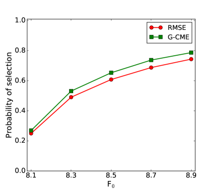
Probability of selection.
We first look at the probability of selection of the correct model version for each indicator; that is, where is computed by counting how many times each indicator chooses the correct model version over the incorrect one, out of the total of cycles. Thus, a random classifier will produce a probability of selection equal to and a perfect classifier will produce one equal to . This allows us to evaluate the reliability of the indicators in terms of model version selection. Then, by repeating the computation for different values of , we deduce the sensitivity of either indicator to the discrepancy - between correct and incorrect model version.
The probabilities of selection are given in Figure 1. The incorrect model versions are simulated with the forcings plotted on the -axis.
Note that the larger the forcing , the easier it should be to select the correct model version over the incorrect one. Therefore, a good model version selection indicator is the one that increases the fastest when is increased.
From Figure 1, we see that the RMSE selects the correct model version over the incorrect one given by with a probability of that is slightly inferior to the G-CME probability of . As the forcing of the incorrect model version increases, both indicators increase their probabilities of selection but the growth of the G-CME indicator is faster.
 |
 |
ROC curves and the Gini coefficient.
The probabilities of selection as computed in Figure 1 only evaluate the ability of the indicators to select one model version over the other. Yet the values of these indicators also provide distances between the two model versions. The greater these distances, the greater the confidence in the corresponding model version selection.
We define the confidence value in the model version selection for the G-CME indicator as the difference between the logarithms of the model evidences, introduced in section 2, namely
| (20) |
with being the G-CME value for the correct model version and the G-CME value for the incorrect one. Similarly, a confidence value is defined for the RMSE, as
| (21) |
with RMSE1, defined in Eq. (19), for the correct model version and RMSE0 for the incorrect one.
In order to evaluate the ability of each indicator to select the correct model version with various levels of confidence, we compute a Receiver (or Relative) Operating Characteristic (ROC) curve. A ROC curve measures the performance of a binary classifier; see, for instance, Metz (1978) for a review of ROC analysis.
In our study, we define the ROC curve as follows. If the confidence value (either or ) is positive, we consider the correct model version to have been selected and the incorrect one if it is negative. Knowing that there is only one correct model version, we define the selection of the latter as a true positive instance and the selection of the incorrect model version as a false positive instance.
Note that, with this definition of the classifier, there is neither a true negative nor a false negative for which a confidence value is obtained. Still, this configuration allows us to define the True Positive Rate (TPR) and the False Positive Rate (FPR), two parametric functions of the threshold , giving the proportion of positives that are correctly identified as such (i.e., when ) and, respectively, the proportion of negatives wrongly identified as positives (i.e., when ). The ROC curve is then displayed by plotting parametrically the TPR() against the FPR() for varying thresholds .
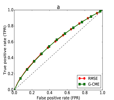
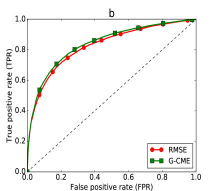
The random classifier has a chance of selection of each model version for every threshold and it will produce a diagonal ROC curve (black dashed line in Figures 2, 4 and 6), namely a straight line between the origin and the point , while a perfect classifier that always selects the correct model version has a ROC curve equal to for and to for .
Figure 2 shows the ROC curves of the model version selection indicator RMSE (solid red line with red circles) and the model version selection indicator G-CME (solid green line with squares), for two incorrect model versions: (a) the one closest to the correct value, i.e. ; and (b) the one farthest from it, i.e. . Both indicators outperform random selection by exhibiting a higher TPR/FPR ratio throughout, for every threshold . As was the case for the probability of selection in Figure 1, the RMSE and the G-CME are almost equally selective for the more difficult case of the incorrect model version in panel (a), while the G-CME indicator slightly outperforms the RMSE for in panel (b).
The Gini (1921) coefficient provides a simple scalar that quantifies the improvement of a given classifier over the random one. This coefficient equals the area between the classifier’s ROC curve and the diagonal of the graph — which is the ROC curve of the random classifier — divided by the area between the latter and the -axis. In other words, . Hence, the Gini coefficient for the random classifier is and the Gini coefficient for a perfect classifier is .
The Gini coefficients corresponding to the ROC curves in Figure 2 are reported in Table 1. In the case of the incorrect model version with , the Gini coefficients of the RMSE and the G-CME are very close, with only a difference in favor of the RMSE. The G-CME outperforms the RMSE in the case of the incorrect model version with : its Gini coefficient is higher by .
To summarize, results so far suggest that the G-CME and the RMSE present comparable selection skills for similar model versions, such as in the case and , but the G-CME converges faster to a perfect classifier as is increased.
4.2.2 CME with domain localization
In the previous subsection, a 40-member ensemble was used to compute the model version selection indicators. However, in geosciences applications, such a big ensemble, with comparable to the state vector size , is quite unrealistic. To mimic a more realistic scenario, we use here a 10-member ensemble, i.e. , in conjunction with localization. Bocquet and Carrassi (2017) have shown that is smaller than the dimension of the unstable–neutral subspace below which localization is mandatory.
Here we use the localization radius , as it produces the smallest RMSEt for the DA process applied to the incorrect model version (not shown here). Since the localization is tuned for the incorrect model version–DA, but left untuned for the correct model version–DA, the analysis errors of the two DAs should be closer to each other than if the localization were tuned independently for each model version. This choice is expected to render the model version selection task harder.
We compare then the selectivity of the DL-CME to the G-CME and the RMSE. Note that unless stated otherwise the same 10-member ensemble is used to compute the three model version selection indicators: DL-CME, G-CME and RMSE. As before, these three model version selection indicators are computed at each of the cycles of the numerical experiment.
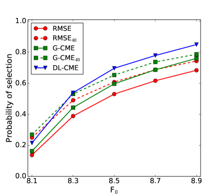
Probability of selection.
Figure 3 shows the probabilities of selection as a function of the incorrect model versions, with , for three model version selection indicators: RMSE, G-CME and DL-CME. The probabilities for the RMSE and the G-CME using the 40-member ensemble, and displayed in Figure 1, are also reported in Figure 3 for comparison.
First, we note that the probabilities of selection for both RMSE and G-CME are lower for than for . This means that the use of a smaller ensemble and no localization in the DA reduces the probabilities of a correct selection by the RMSE and the G-CME and is a direct consequence of the reduced accuracy of the DA in performing the state estimate. However, the convergence rate of the G-CME with is faster than for G-CME40 and, when , they select the correct model version with almost the same accuracy.
The key result, though, is related to the effect of localization. We see that for the same ensemble size , the DL-CME outperforms both the RMSE and the G-CME indicators. Notably, the DL-CME with selects the correct model version with a higher probability than the G-CME with , except for the case of smallest error in model version definition, i.e. for .
 |
 |
ROC curves and the Gini coefficient.
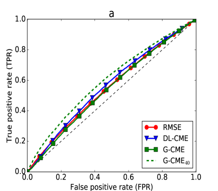
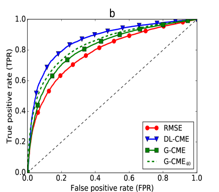
The previous conclusion is confirmed by the ROC curves in the cases of the incorrect model versions with and that are plotted, respectively, in Figures 4(a, b). The ROC curves of G-CME40 have also been plotted in Figure 4 for reference and benchmark. The DL-CME has a TPR/FPR ratio that is larger than the G-CME for both incorrect model versions. This result represents a substantial improvement in the computation of the CME.
In the difficult case of , the DL-CME with is not as accurate in model version selection as the G-CME40 but, as previously stated, the use of large ensembles is most often not feasible for models of a realistic size. Interestingly, in the case of , the DL-CME still provides a more accurate model version selection than the G-CME40.
These results are confirmed by the corresponding Gini coefficient listed in Table 2. In the case , the DL-CME model version selection skill outperforms the G-CME40, even though the DA performance for state estimation in terms of RMSEt is better when with no localization than with localization (not shown).
4.2.3 Sensitivity to the localization radius
Even though only the DL-CME takes into account the localization, the G-CME and the RMSE are also potentially sensitive to the localization radius since they are based on the output of a DA cycle that uses localization. The way the three model version selection indicators respond to the localization radius is examined in Figure 5.
The experimental setup is identical to that in the previous subsections and the ensemble size is . The localization radius is shown on the -axis; while the Gini coefficient for each model version selection indicator is plotted on the -axis. Superimposed on Figure 5 are the RMSEt curves for the DA with the correct and the incorrect model version, in solid and dashed black lines, respectively.
The results in Figure 5 confirm, once more, the superiority of the two CME indicators over the RMSE. They also confirm the improvement achieved by taking into account domain localization in the CME computation, i.e., the better model version selection by the DL-CME with respect to the G-CME; both improvements are present across all localization radii.
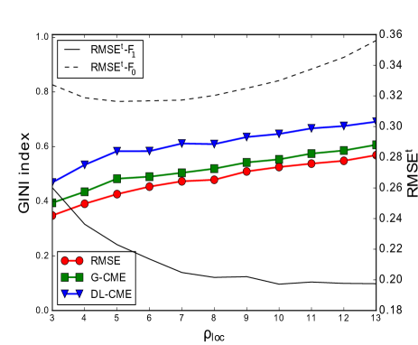
It is, moreover, worth noting that the sensitivity of all three indicators to the localization radius is small. For all the indicators, the Gini coefficient increases slowly with . This increase can be explained by the difference in performance of the DA’s state estimation. Indeed the difference between the two RMSEt curves also increases with the localization radius. Hence, the selection between the two DA-produced ensembles becomes easier as increases. The key result, however, is that the sensitivities of the two CME indicators are approximately the same. Thus, taking the localization into account in the CME computation should improve the CME’s model version selection skill, whatever the value of the localization radius.
 |
 |
4.2.4 Dependence on the evidencing window
In all previous experiments, the model version selection indicators are computed over an evidencing window , i.e., using only one DA cycle. This choice was made to assess the indicators’ performance in the most difficult setting. Indeed, selecting a model version based on static information alone is a difficult task that is not usually required in geosciences applications. In the latter, one may want to select the most accurate model representation of a meteorological event or a climatological time span, seen as a “video loop” or a “full-length movie”, respectively (Ghil, 1997). We thus want now to evaluate the indicators in a more realistic setting, by comparing the correct model version, with , and the most incorrect one being considered, with , over larger evidencing windows, namely and .
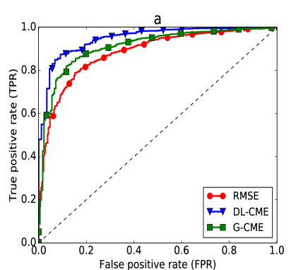
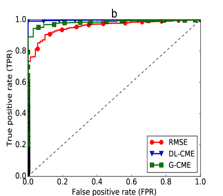
The ROC curves obtained for these two experiments, with and , are displayed in Figures 6(a) and (b), respectively. Comparing these curves with these for K=1 of Figure 4(b), we see that increasing the evidencing window improves the selection skills of all the indicators as they converge to the perfect classifier. This behavior is consistent with the results obtained by Carrassi et al. (2017) in the absence (of the need) of localization.
Moreover, in the case , the DL-CME still outperforms the RMSE and the G-CME. In the case , both CME indicators remain more accurate than the RMSE, while the DL-CME is almost achieving a perfect selection. Altogether, the results in Figures 4(b), 6(a) and 6(b) indicate that when is increased all indicators converge to the perfect classifier. It follows that, for small and medium evidencing windows, the DL-CME outperforms the CME with no localization and the RMSE, but larger evidencing windows, when feasible computationally, may allow all indicators to show similar selection skills.
5 Numerical experiments with an atmospheric model
This section presents the first implementation of the CME approach for an intermediate-complexity model. The numerical experiments herein confirm the benefits of applying CME in general, and DL-CME in particular, as a model version selection indicator for larger models.
5.1 Experimental setup
5.1.1 The SPEEDY model
We use an atmospheric general circulation model (AGCM) based on a spectral primitive-equation dynamic core that resolves the large-scale dynamics of the atmosphere. The model was developed at the International Center for Theoretical Physics (ICTP) and it is referred to as the ICTP AGCM or the Simplified Parameterizations, primitivE-Equation DYnamics (SPEEDY) model (Molteni, 2003; Kucharski, 2006). With its dynamical core and its simplified physical parameterization schemes, SPEEDY simulates successfully some of the complex physics described by state-of-the-art AGCMs, while maintaining a low computational cost (Neelin et al., 2010). Hence, its intermediate-level complexity — between low-order models and high-end AGCMs — has made SPEEDY an important test bed for model development studies (e.g., Kucharski and Molteni, 2003; Haarsma, 2003; Bracco, 2004; Kucharski, 2006) and for evaluating DA methodology (Miyoshi, 2005; Miyoshi and Yamane, 2007).
The model’s spectral dynamical core (Molteni, 2003) uses a hydrostatic, -coordinate, spectral-transform formulation in the vorticity-divergence form described by Bourke (1974). The configuration we use here is described by Miyoshi (2005) and it has a spectral resolution of T30L7, i.e., a horizontal spectral truncation at spherical wavenumber 30 and 7 vertical layers. It has a vertical -coordinate and it computes four physical variables in every vertical layer: zonal wind , meridional wind , temperature , and relative humidity , as well as one surface variable, in the lowest vertical layer, namely surface pressure .
The simulated values for each vertical field are given on a 96 long. 48 lat. horizontal grid. A summary description of SPEEDY, including its simplified physical parametrizations, is available in the appendix of Molteni (2003). We provide here a detailed description of its convection parametrization, since the purpose of the present section is to perform parameter selection between two values of a convective parameter. In a sense, CME and DL-CME can be viewed also in the framework of the parameter estimation problem (Ghil and Malanotte-Rizzoli, 1991; Ghil, 1997; Navon, 1997; Carrassi et al., 2017).
 |
 |
5.1.2 The model’s convection parametrization
SPEEDY’s convection scheme is a simplified version of the mass-flux scheme developed by Tiedke (1993). The scheme simulates the balance of the updraft of the saturated air and the large-scale downward motion in between the planetary boundary layer (PBL) and the top-of-convection (TCN) layer. While the updraft of saturated air is triggered above the PBL, the detrainment only takes place in the TCN layer. In addition, the convection scheme simulates an exchange of moisture between the PBL and the layers above it.
SPEEDY’s simplified convection parametrization may roughly be summarized by three main steps: an activation of the convection scheme, its closure and an exchange mechanism between the intermediate layers. In particular, the closure of the scheme requires the convective moisture tendency in the PBL to be equivalent to a relaxation of humidity towards a prescribed threshold with a relaxation time equal to ; in our study, the parameter of interest is precisely . This parameter has a straightforward physical interpretation since it controls the speed of the vertical mixing associated with moist convection, and its interest lies in its impact on the global–scale circulation.
The correct parameter value, namely the value set in SPEEDY to create a ‘true’ trajectory — in the sense defined in sections 2 and 4 — is hr. Meanwhile, the incorrect parametrization here will use the relaxation time hr. The objective is to be able to select the correct parameter over the incorrect one, based on the observation of what is deemed to be the true trajectory in the present, “dizygotous-twin” setting; see, for instance, Ghil and Malanotte-Rizzoli (1991) for an explanation of the distinctions between identical-twin, dizygotous-twin and real-observations setup in DA studies. The DA formulation needed to do the parameter selection in this setup is presented in the next subsection.
5.1.3 The DA implementation
As in the L95 experiments of section 2, a true trajectory is generated using the correct parameter value of hr. From this trajectory a set of observations are derived and made available every 6 hr. This DA configuration was adapted for SPEEDY by Miyoshi (2005).
The observed physical quantities are the 5 prognostic variables , , , , throughout the model’s 7 layers, and the surface pressure . All variables are observed every four gridpoint, yielding observations for , , , and observations for the surface pressure. The observation error variances, used to create the observations in the DA process, are:
The experiment lasted 6 months, from 1 January to 30 June 1983. The results for the spin-up time of DA cycles (i.e., the 1st month) were discarded, and the diagnostics were calculated for the DA cycles of 1 February through 30 June.
The DA is performed using the LETKF (cf. section 3.1.2) with N=50 ensemble members and with the domain localization introduced by Hunt et al. (2007), Miyoshi and Yamane (2007), and Greybush et al. (2011): localization domains are selected and the observation error covariance sub-matrix is multiplied, for each , by the inverse of a smoothing function, as explained in section 3.1. In this study, we use the implementation proposed by Miyoshi et al. (2007) and apply as a smoothing function, in the three–dimensional physical space, the Gaussian function
| (22) |
here is the distance between the localization domain’s center and the observations, while is the localization radius, and both quantities have a horizontal and a vertical component. The horizontal component of is taken equal to 700 km, while its vertical component is defined in terms of log-pressure coordinates and corresponds to approximately 4 km.
Note that, in the following, the DL-CME results are computed for specific variables, i.e., we assume that only these variables have been observed. This computation is identical to the computation of the CME for an observation subvector, as discussed in section 3.2.1.
For an evidencing window that has length , the required computation of the pdf of the system’s state, conditioned on this particular observation subvector leads to a DA run that does not converge. Hence, we approximate once again this conditional pdf by the original posterior pdf which consists in directly applying the EnKF-formulation to the observation vector reduced to a specific variable using Eq. (14).
5.2 Model version selection problem
We now focus, as explained in section 5.1.2, on determining which value of the relaxation parameter (6 or 9 hrs) is more appropriate to describe the atmospheric evolution simulated during the 5 months of the experiment. Recall that the value hrs is the one used to simulate the reference truth from where the observations are sampled. The model version selection is here a parameter identification problem and, again, is carried out with the RMSE, the G-CME, and the DL-CME as indicators.
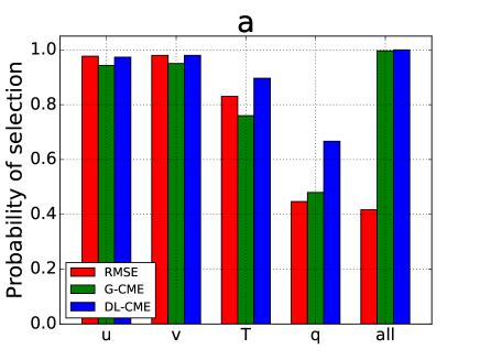
The indicators are first computed on the evidencing window , i.e., on a single DA cycle then averaged over the 5–month interval. The results in terms of selection probability obtained on the various variables are shown in Figure 7(a).
As mentioned in section 5.1.2, the value of the relaxation time plays an important role in the global-scale circulation: it intensifies, for instance, the mesoscale circulations associated with deep convection which then affects the extent and intensity of the Hadley and Walker cells (see for instance Donner et al., 2001). This physical connection is confirmed by the results of the three model version selection indicators when using observations of the variables or alone. Indeed, for either of these two variables, the indicators select the correct parameter with high probability.
Note that the RMSE outperforms the G-CME selecting skills on these two variables. However, taking into account localization, i.e., using the DL-CME, improves the selection skills of the CME and provides equally high selection probabilities as the RMSE does. Moreover, when only T-data are used, the DL-CME identifies the correct parameter with the highest probability. The humidity variable, , is the variable least impacted by the variation of . Yet, the DL-CME is the best to emphasize the improvement of the correct parameter on the humidity representation. Finally, when using all observations, both CMEs fully discriminate between the two model versions whereas the RMSE only partially does.
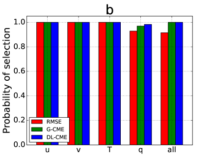
A more realistic setting is to use a longer evidencing window, taken now as , which corresponds to 3 days. The results of this experiment are shown in Figure 7(b), and they confirm that increasing improves the selection skills of all indicators. The humidity is still the most difficult variable to discriminate the two model versions from. Yet, the DL-CME remains the best selector, strongly selective for all variables, both separately and together. Moreover, when using all observations, the RMSE fails to systematically recognize the correct model version from the incorrect one.
From a practical stand-point, the latter result indicates that if, for instance, one’s goal is to determine which of two model versions is most likely responsible for a three-day weather event that was fully observed, the DL-CME is more likely than the RMSE to provide the correct answer.
 |
 |
5.3 Mapping model evidence
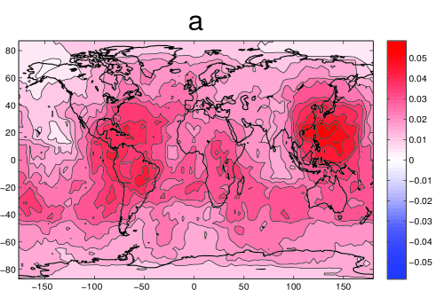
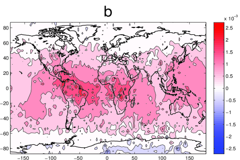
Local CMEs, defined by Eq. (14), also provide a spatial representation of model evidence. This is exploited in Figure 8 that shows the spatial differences between the correct and the incorrect parametrization using all observations.
Note that the distinct information conveyed by these two maps — the local RMSE differences in panel (a) and the local CME differences in panel (b) — is not necessarily contradictory but rather complementary since the RMSE is the Euclidean distance between the DA forecast and the observations while the local CME can be seen as a distance between the same two quantities but smoothed by the uncertainties that surround them.
Indeed, the local RMSE reveals a significant difference between the two model versions all over the globe while the local CME shows that this difference mainly impacts the low latitude regions. Also, some of the regions that are strongly impacted by the incorrect parameter according to the RMSE, are not so according to the local CME. For instance, the differences emphasized by the RMSE in the region off the coast of China are sensibly smaller according to the local CMEs. This would suggest that, although the DA forecast produced by the incorrect model version does not fit the observations as well as the one produced by the correct model version, the uncertainties generated in this region mitigate the quality of the correct model version’s representation of this region.
6 Concluding remarks
6.1 Summary and conclusions
Carrassi et al. (2017) have introduced the contextual model evidence (CME) as a powerful indicator for model version selection and for attribution of climate related events. They also have provided analytic ways to compute this indicator by using a hierarchy of ensemble-based data assimilation (DA) algorithms and have shown its efficiency.
When applied to large-dimensional models, ensemble-based DA requires localization techniques in order to mitigate the spurious effect of under-sampling. The present study focused on adapting the CME’s EnKF-formulation to the use of a specific localization technique, namely domain localization.
In section 3.2.1, we have shown how to compute local CMEs as the CMEs of an observation subvector. This idea led to an EnKF-formulation of the local CME, given by Eq. (14), subject to very few simplifying assumptions. Combining local CMEs for each grid point, we introduced in Eq. (15) a heuristic model version selection indicator called the domain-localized CME (DL-CME). This DL-CME formulation allows one to estimate model evidence in a consistent and routine way by using localized DA with large-dimensional problems.
We implemented the DL-CME formulation — along with the global CME’s EnKF-formulation called global CME (G-CME) and the root mean square error (RMSE), defined by Eq. (19) — on two atmospheric models: the 40-variable mid-latitude atmospheric dynamics model (L95: Lorenz and Emanuel, 1998) and the simplified global atmospheric SPEEDY model (Molteni, 2003), in sections 4 and 5, respectively. The main objective of the numerical experiments in these two sections was to assess the performance of the three approaches so defined — the RMSE, the G-CME and the DL-CME — in increasingly harder model version selection problems.
In section 4, the numerical experiments based on the L95 model were used to compare the three model version selection indicators for varying model forcings , as well as with respect to the localization radius and to the length of the evidencing window. In general, both CME indicators, G-CME and DL-CME, are more accurate than the RMSE; see Figures 1–6. Moreover, the DL-CME outperforms systematically the G-CME regardless of the length of the localization radius, cf. Figure 5.
In the 40-ensemble member localization-free experiment, the G-CME increasingly outperforms the RMSE when the difference between the model forcings is increased; see Figures 1-2. When the number of ensemble members is reduced to 10, hence making localization necessary, the G-CME is still more accurate than the RMSE. With the same ensemble size, the DL-CME is even more accurate than the G-CME which indicates the impact of consistently using localization in both the DA state estimation procedure and in the CME computation. Remarkably, DL-CME, with a 10-member ensemble and localization, produces better selection probabilities than G-CME with a 40-member ensemble and no localization, at least when the discrepancy between the correct and incorrect forcing is large enough, cf. Figures 3-4.
The sensitivity of the model version selection skill to the localization radius is approximately the same for all indicators, meaning that the improvement of the DL-CME over the two other indicators is almost independent of the localization radius, cf. Figure 5 . This independence is highly desirable, given the computational cost of tuning the radius. In particular, the DL- CME is clearly the most accurate indicator for small evidencing windows. For larger windows, the performances of the DL-CME and the G-CME become almost identical and do remain higher than the RMSE’s performance, see Figure 6.
In section 5, model version selection was carried out for a more realistic problem. We formulated two parametrizations of the convection in the SPEEDY model by varying the convective relaxation time . The selecting skills of the RMSE, the G-CME and the DL-CME were assessed on all physical model variables, both separately and together.
Over a single DA-cycle, the DL-CME and the G-CME are fully selective on all variables combined. The DL-CME, though, is the best selection indicator on all four model variables — , , and — separately, whether for a single DA-cycle or a large evidencing window, , as shown in Figure 7.
Local CMEs provide, in addition, a spatial view of model evidence, cf. Figure 8. This spatial view can provide precious information on the impacts of the correct and incorrect parametrizations on the physical evolution of the large-scale atmospheric flow.
In summary, while the DL-CME displays the best performance in terms of model version selection, the spatial plots of local CME can help identifying the spatial regions and the physical variables where the incorrect model version misfits the observations. Beyond model version selection problems, this feature can be used to bring precious information in order to help understanding the causal chain leading to meteorological or climatological events as well as designing target observations/areas for that purpose.
6.2 Future directions
A first line of future investigations should focus on strengthening the theoretical foundation of the CME. Indeed, several theoretical issues are yet to be addressed. For instance, simulating model error and taking it into account in both the DA process and in the CME computation could improve significantly the CME’s model version selection skill. The DA community is still conducting active research on the best ways to incorporate model error in DA methodology (e.g., Dee, 1995; Raanes et al., 2015; Carrassi and Vannitsem, 2016; Harlim, 2017). This research has the potential to improve significantly the accuracy of the DA product improving therewith the CME estimation. Moreover, taking into account model error in the CME computation itself could also have an impact in the CME’s model version selection abilities.
A second potential limitation of the CME method is the accuracy of the CME estimation when computed with a sparsely observed system. This limitation obviously depends on the accuracy of the assimilation itself. However, as long as the assimilation is possible – i.e. as long as the spatial and temporal density of the observations is sufficient for the system to be observable – and the two compared model versions have the same observation system, one can assume that they will be similarly impacted. A study of the observation system’s impact on the CME’s model version selection skill and, more generally, on the CME estimation should be conducted in the future..
Another theoretical issue requiring investigation is the derivation of an exact global indicator based on local CMEs that could outperform the global heuristic indicator proposed in this article, the DL-CME. These theoretical challenges are part of the authors’ current research program.
A second line of investigations should focus on broadening the applications of the CME approach. The realism and the complexity of the models considered needs to be increased. Indeed, the CME approach allows one to compare model versions that differ from one another by the values of a set of parameters.
In the numerical experiments presented here, the model versions differed only by a parameter’s scalar value, yet one may wish to consider two complex model versions that differ by by the values of a large set of parameters or by an entire two-dimensional forcing field, like the sea surface temperatures for an atmospheric model. For instance, in currently ongoing work, the authors are using the CMEs to identify the best turbulence closures among a number of full parametrization schemes.
At the same time, application of the CME approach should be widened from model version selection to other purposes, such as causal attribution of observed changes. In particular, it seems worth investigating the potential of the spatial representation of local CMEs for diagnosing causality in a geoscientific system, as proposed by Hannart et al. (2016b).
Acknowledgments
We acknowledge discussions with the other members of the DADA team (Philippe Naveau, Aurélien Ribes and Manuel Pulido). We also wish to acknowledge personal communications with Pr. P.J. Van Leeuwen which led to clarifications of the manuscript.
This research was supported by grant DADA from the Agence Nationale de la Recherche (ANR, France: All authors), and by Grant N00014-16-1-2073 of the Multidisciplinary University Research Initiative (MURI) of the US Office of Naval Research (MG). A. Carrassi has been funded by the project REDDA of the Norwegian Research Council (contract number 250711). J. Ruiz has been funded by the project PICT2014-1000 of the Argentinian National Agency for Scientific Research Promotion. CEREA is a member of the Institute Pierre Simon Laplace (IPSL).
Appendix A
Alternative implementation of the global CME (G-CME)
The G-CME implementation was first presented in Carrassi et al. (2017) for the CME formulation based on the En-4D-Var DA method. This implementation makes the assumption that the observation error covariance matrix R is diagonal. This assumption is strong but often verified in geosciences applications.
Implementing Eq. (8) requires to derive: (i) the determinant term ; (ii) the weighted sum of squares . We deal with each two terms separately.
First, the computation of the determinant term can be greatly simplified by application of Sylvester’s determinant rule (i.e., for any two rectangular matrices A and B of conformable sizes). We have
| (23) | ||||
where . with , the normalized forecast anomalies such that . Note that R is diagonal in general thus its determinant is easy to compute.
Under Eq. (2), one sees that boils down (after the one off computation of ) to the computation of which is a much smaller determinant of dimension (size of the ensemble) instead of dimension (size of the observation vector).
Second, the computation of the weighted sum of squares can also be greatly simplified by application of the Sherman-Morrison-Woodbury formula. We have
| (24) | ||||
It follows
| (25) | ||||
with .
Appendix B
Derivation of the CME formulation using background covariance localization
Background covariance localization (also called Schur localization) consists in restraining the spatial impact of the empirical forecast error covariances. Indeed, the ensemble size is smaller than the model’s state dimension and thus the ensemble-based covariance is subsampled by construction. This subsampling may lead to spurious correlations. This issue can be partly overcome by removing the unrealistic correlations. Background covariance localization performs this removal by applying to the forecast error covariance matrix a Schur product (i.e., a pointwise multiplication) with a smoothing correlation matrix
| (26) |
where the correlation matrix coefficients are defined by , for a smoothing function.
The smoothing function we use is a short-ranged predefined correlation function , based on the Gaspari-Cohn function (Gaspari and Cohn, 1999), for the localization radius ,
| (30) |
Based on the background covariance localization, a new CME formulation can be derived. We call this formulation: the Global Localized CME (GL-CME). The GL-CME respects the original formulation Eq. (8), i.e., is computed for the entire observation vector, while taking into account the regularized forecast error covariance matrix in the term
| (31) |
In this case, the CME computation remains quite straightforward. However, concerning the computational cost, the regularization does not change the size of . The computational cost is as heavy as the original EnKF-formulation which adds to the cost of the application of a Schur product, making this formulation not directly tractable in high dimensions. To do so, additional sophisticated techniques are required.
References
- Ando (2010) Ando T. 2010. Bayesian Model Selection and Statistical Modeling. CRC Press, Boca Raton, FL
- Akaike (1974) Akaike H. 1974. A new look at the statistical model identification. Autom. Contr., IEEE Trans., 19: 716-723
- Asch et al. (2016) Asch, M., Bocquet M., Nodet M. 2016. Data Assimilation: Methods, Algorithms, and Applications. Fundamentals of Algorithms. SIAM, Philadelphia.
- Balgovind et al. (1983) Balgovind, R., Dalcher A., Ghil M., Kalnay E. 1983) A stochastic-dynamic model for the spatial structure of forecast error statistics. Mon. Wea. Rev., 111, 701–722.
- Baum et al. (1970) Baum LE., Petrie T., Soules G., Weiss N. 1970. A maximization technique occurring in the statistical analysis of probabilistic functions of Markov chains. The Annals of Mathematical Statistics, 41:164-171.
- Bennett (1992) Bennett AF.. 1992. Inverse Methods in Physical Oceanography. Cambridge University Press, Cambridge, UK and New York, NY, USA.
- Bishop et al. (2001) Bishop CH., Etherton BJ., Majumdar SJ. 2001. Adaptive sampling with the ensemble transform Kalman filter. Part I: Theoretical aspects. Mon. Wea. Rev., 129: 420-436.
- Bocquet (2016) Bocquet M.. 2016. Localization and the iterative ensemble Kalman smoother. Q. J. R. Meteorol. Soc., 142: 1075-1089.
- Bocquet and Carrassi (2017) Bocquet M., Carrassi A. 2017. Four-dimensional ensemble variational data assimilation and the unstable subspace. Tellus A, 69: 1304504.
- Bourke (1974) Bourke, W.. 1974. A multilevel spectral model. I. Formulation and hemispheric integrations. Mon. Wea. Rev., 102: 687-701.
- Bracco (2004) Bracco A., Kucharski F., Kallumal R., Molteni F. 2004. Internal variability, external forcing and climate trends in multi-decadal AGCM ensembles. Clim. Dyn., 23: 659-678
- Buehner et al. (2010) Buehner M., Houtekamer PL., Charette C., Mitchell HB. 2010. Intercomparison of variational data assimilation and the ensemble Kalman filter for global deterministic NWP. Part I: Description and single-observation experiments. Mon. Wea. Rev., 138: 1550-1566.
- Burnham and Anderson (2002) Burnham KP., Anderson DR. 2002. Model selection and inference: A practical information-theoretic approach. Springer: New York, 2nd edition.
- Carrassi and Vannitsem (2016) Carrassi A., Vannitsem S. 2016. Deterministic treatment of model error in geophysical data assimilation. In Mathematical Paradigms of Climate Science, Springer: 175-213.
- Carrassi et al. (2017) Carrassi A., Bocquet M., Hannart A., Ghil M. 2017. Estimating model evidence using data assimilation. Q. J. R. Meteorol. Soc., 143: 866–880.
- Carrassi et al. (2018) Carrassi, A., Bocquet M., Bertino L., Evensen G. 2018. Data assimilation in the geosciences: An overview of methods, issues, and perspectives. WIREs Clim. Change 2018, 9(5).
- Carson et al. (2017) Carson J, Crucifix M., Preston S., Wilkinson RD. 2017. Bayesian model selection for the glacial-interglacial cycle. Journ. of the Roy. Stat. Soc.: Series C (Applied Statistics).
- Cressman (1959) Cressman, G.P. 1959 An operational objective analysis system. Mon. Wea. Rev., 87: 367-374.
- Daley (1991) Daley R. 1991. Atmospheric data analysis. Cambridge University Press, Cambridge, United Kingdom.
- Dee (1995) Dee DP. 1995. On-line estimation of error covariance parameters for atmospheric data assimilation. Mon. Wea. Rev., 123: 1128-1145.
- Del Moral (2004) Del Moral P. 2004. Feynman-Kac formulae: genealogical and interacting particle systems with applications. Sringer: New York.
- Donner et al. (2001) Donner LJ., Seman CJ., Hemler RS., Fan S. 2001. A cumulus parameterization including mass fluxes, convective vertical velocities, and mesoscale effects: Thermodynamic and hydrological aspects in a general circulation model. Journ. of clim., 14: 3444-3463.
- Elsheikh et al. (2014a) Elsheikh A, Hoteit I., Wheeler M. 2014a. Efficient bayesian inference of subsurface flow models using nested sampling and sparse polynomial chaos surrogates. Comput. Methods Appl. Mech. Engrg., 269: 515-537.
- Elsheikh et al. (2014b) Elsheikh A, Wheeler M., Hoteit I. 2014b. Hybrid nested sampling algorithm for Bayesian model selection applied to inverse subsurface flow problems. J. Comput. Phys., 258: 319-337.
- Evensen (2009) Evensen G. 2009. Data Assimilation: The Ensemble Kalman Filter. Springer- Verlag/Berlin/Heildelberg, second edn.
- Gaspari and Cohn (1999) Gaspari G., Cohn SE. 1999. Construction of correlation functions in two and three dimensions. Quart. J. Roy. Meteor. Soc., 125: 723-757.
- Ghil et al. (1979) Ghil, M., Halem M., Atlas R. 1979. Time-continuous assimilation of remote-sounding data and its effect on weather forecasting. Mon. Wea. Rev., 107: 140–171.
- Ghil (1997) Ghil M. 1997. Advances in sequential estimation for atmospheric and oceanic flows. J. Meteor. Soc. Japan, 75: 289-304.
- Ghil and Malanotte-Rizzoli (1991) Ghil M., Malanotte-Rizzoli P. 1991. Data assimilation in meteorology and oceanography. Adv. Geophys., 33: 141-266.
- Gini (1921) Gini C. 1921. Measurement of inequality of incomes. Econ. J., 31: 124-126.
- Greybush et al. (2011) Greybush SJ., Kalnay E., Miyoshi T., Ide K., Hunt BR. 2011. Balance and ensemble Kalman filter localization techniques. Mon. Wea. Rev., 139: 511-522.
- Haarsma (2003) Haarsma RJ., Campos EJD., Molteni F. 2003. Atmospheric response to South Atlantic SST dipole. Geophys. Res. Lett., 30.
- Hamill et al. (2001) Hamill, TM., Whitaker JS., Snyder C. 2001. Distance-dependent filtering of background error covariance estimates in an ensemble Kalman filter. Mon. Wea. Rev., 129: 2776-2790.
- Harlim (2017) Harlim J. 2017. Model error in data assimilation. In Nonlinear and Stochastic Climate Dynamics, Franzke CLE. and TJ. O’Kane (eds.) Cambridge University Press: Cambridge, UK.
- Hannart et al. (2016a) Hannart A., Pearl J., Otto F.E.L., Naveau P., Ghil M. 2016a. Causal counterfactual theory for the attribution of weather and climate-related events. Bull. Am. Meteorol. Soc., 97: 99-110.
- Hannart et al. (2016b) Hannart A., Carrassi A., Bocquet M., Ghil M., Naveau P., Pulido M., Ruiz J., Tandeo P. 2016b. DADA: data assimilation for the detection and attribution of weather and climate-related events. Climatic Change, 136: 155-174.
- Houtekamer and Mitchell (2001) Houtekamer PL., Mitchell HL. 2001. A sequential ensemble Kalman filter for atmospheric data assimilation. Mon. Wea. Rev., 129: 123-137.
- Hunt et al. (2007) Hunt B., Kostelicj EJ., Szunyogh I. 2007. Efficient data assimilation for spatiotemporal chaos: A local ensemble transform Kalman filter. Physica D, 230: 112-126.
- Ide et al. (1997) Ide, K., Courtier P., Ghil M., Lorenc A. 1997. Unified notation for data assimilation: Operational, sequential and variational. J. Meteor. Soc. Japan, 75: 181-189.
- Kalnay (2003) Kalnay E. 2003. Atmospheric modeling, data assimilation and predictability. Cambridge university press.
- Kucharski and Molteni (2003) Kucharski F., Molteni F. 2003. On non-linearities in a forced North Atlantic Oscillation. Clim. Dyn., 21: 677-687.
- Kucharski (2006) Kucharski F., Molteni F., Bracco A. 2006. Decadal interactions between the western tropical Pacific and the North Atlantic Oscillation. Clim. Dyn., 26: 79-91.
- Lermusiaux (2006) Lermusiaux PFJ. 2006. Uncertainty estimation and prediction for interdisciplinary ocean dynamics. J. Comp. Phys., 217: 176-199.
- Lorenz (1963) Lorenz EN. 1963. Deterministic nonperiodic flow. J. Atmos. Sci., 20: 130-141.
- Lorenz (1996) Lorenz EN. 1996. Predictability: a problem partly solved. Seminar on Predictability, 4–8 September 1995, European Centre for Medium-range Weather Forecasting, Shinfield Park, UK, pp. 1–18.
- Lorenz and Emanuel (1998) Lorenz EN., Emanuel KA. 1998. Optimal sites for supplementary weather observations: simulation with a small model. J. Atmos. Sci., 55: 399-414.
- Metz (1978) Metz CE. 1978. Basic principles of ROC analysis. Semin. Nucl. Med., 8: 283-298.
- Molteni (2003) Molteni F. 2003. Atmospheric simulations using a GCM with simplified physical parameterizations. I: model climatology and variability in multi-decadal experiments. Clim. Dyn., 20: 175-191.
- Miyoshi (2005) Miyoshi T. 2005. Ensemble Kalman filter experiments with a primitive-equation global model. Ph.D. dissertation, University of Maryland, 197 pp.
- Miyoshi and Yamane (2007) Miyoshi T., Yamane S. 2007. Local ensemble transform Kalman filtering with an AGCM at a T159/L48 resolution. Mon. Wea. Rev., 135: 3841-3861.
- Miyoshi et al. (2007) Miyoshi T., Yamane S., Enomoto T. 2007. Localizing the error covariance by physical distances within a Local Ensemble Transform Kalman Filter (LETKF). SOLA, 3: 89-92
- Navon (1997) Navon I.M. 1997. Practical and theoretical aspects of adjoint parameter estimation and identifiability in meteorology and oceanography. Dynamics of Atmospheres and Oceans, 27, no 1-4: 55-79.
- Neelin et al. (2010) Neelin JD., Bracco A., Luo H., McWilliams JC., Meyerson JE. 2010 Considerations for parameter optimization and sensitivity in climate models. Proc. Natl. Acad. Sci. USA, 107: 21349-21354.
- Otsuka and Miyoshi (2015) Otsuka S., Miyoshi T. 2015. A Bayesian optimization approach to multimodel ensemble Kalman filter with a low-order model. Mon. Wea. Rev., 143: 2001-2012.
- Ott et al. (2002) Ott E., Hunt BR., Szunyogh I., Corazza M., Kalnay E., Patil DJ., Yorke A., Zimin AV., Kostelich EJ. 2002. Exploiting local low dimensionality of the atmospheric dynamics for efficient ensemble Kalman filtering. No. physics/ 0203058.
- Ott et al. (2004) Ott, E., Hunt BR., Szunyogh I., Zimin AV., Kostelich EJ., Corazza M., Kalnay E., Patil DJ., Yorke A. 2004. A local ensemble Kalman filter for atmospheric data assimilation. Tellus A, 56: 415-428.
- Raanes et al. (2015) Raanes PN, Carrassi A., Bertino L. 2015. Extending the square root method to account for additive forecast noise in ensemble methods. Mon. Wea. Rev., 143: 3857-3873.
- Reich and Cotter (2015) Reich S, Cotter C. 2015. Probabilistic Forecasting and Bayesian Data Assimilation. Cambridge University Press, Cambridge, United Kingdom.
- Saha et al. (2010) Saha S., Shrinivas M., Pan HL., Wu X., Wang J., Nadiga S., Tripp P., Kistler R., Woollen J., Behringer D. and others. 2010. The NCEP Climate Forecast System Reanalysis. Bull. Amer. Meteor. Soc., 91: 1010-1057.
- Saha et al. (2014) Saha S., Shrinivas M., Wu X., Wang J., Nadiga S., Tripp P., Behringer D., Hou YT., Chuang HY., Iredell M. and others. 2014. The NCEP Climate Forecast System version 2. J. Climate, 27: 2185-2208
- Sakov and Bertino (2011) Sakov P., Bertino L. 2011. Relation between two common localisation methods for the EnKF. Comput. Geosci., 15: 225-237.
- Sakov et al. (2012) Sakov P., Counillon F., Bertino L., Lisaeter KA., Oke PR., Korablev A. 2012. Topaz4 : an ocean-sea ice data assimilation system for the north atlantic and arctic. Ocean Sci., 8: 633-656.
- Särkkä (2013) Särkkä S. 2013. Bayesian filtering and smoothing (Vol. 3). Cambridge University Press.
- Schwarz (1978) Schwarz G. 1978. Estimating the dimension of a model. Ann. of Stat., 6: 461-464.
- Szunyogh et al. (2008) Szunyogh I., Kostelich EJ., Gyarmati G., Kalnay E., Hunt BR., Ott E., Satterfield E., Yorke JA. 2008. A local ensemble transform Kalman filter data assimilation system for the NCEP global model. Tellus A, 60: 113-130.
- Tiedke (1993) Tiedke M. 1993. A comprehensive mass flux scheme for cumulus parametrization in large-scale models. Mon. Wea. Rev., 117: 1779-1800.
- Whitaker et al. (2008) Whitaker JS., Hamill TM., Wei X., Song Y., Toth Z. 2008. Ensemble data assimilation with the NCEP global forecast system. Mon. Wea. Rev., 136: 463-482.
- Winiarek et al. (2011) Winiarek V., Vira J., Bocquet M., Sofiev M., Saunier O. 2011. Towards the operational estimation of a radiological plume using data assimilation after a radiological accidental atmospheric release. Atmos. Environ. 45: 2944-2955.