Orbits for eighteen visual binaries and two double-line spectroscopic binaries observed with HRCAM on the CTIO SOAR 4m telescope, using a new Bayesian orbit code based on Markov Chain Monte Carlo

Abstract

We present orbital elements and mass sums for eighteen visual binary stars of spectral types B to K (five of which are new orbits) with periods ranging from 20 to more than 500 yr. For two double-line spectroscopic binaries with no previous orbits, the individual component masses, using combined astrometric and radial velocity data, have a formal uncertainty of $\sim 0.1M_{\odot}$. Adopting published photometry, and trigonometric parallaxes, plus our own measurements, we place these objects on an H-R diagram, and discuss their evolutionary status. These objects are part of a survey to characterize the binary population of stars in the Southern Hemisphere, using the SOAR 4m telescope+HRCAM at CTIO. Orbital elements are computed using a newly developed Markov Chain Monte Carlo algorithm that delivers maximum likelihood estimates of the parameters, as well as posterior probability density functions that allow us to evaluate the uncertainty of our derived parameters in a robust way. For spectroscopic binaries, using our approach, it is possible to derive a self-consistent parallax for the system from the combined astrometric plus radial velocity data (“orbital parallax”), which compares well with the trigonometric parallaxes. We also present a mathematical formalism that allows a dimensionality reduction of the feature space from seven to three search parameters (or from ten to seven dimensions - including parallax - in the case of spectroscopic binaries with astrometric data), which makes it possible to explore a smaller number of parameters in each case, improving the computational efficiency of our Markov Chain Monte Carlo code.

=6

1 Introduction

The laws of physics, applied to stars in hydrostatic equilibrium, indicate, through the well-known Vogt-Russell theorem (Kahler (1972); Kippenhahn et al. (2012)), that the most fundamental parameter determining the evolutionary path and the internal structure of stars of a given chemical composition is their initial mass content (for a general review see Massey et al. (2001), and the textbooks by Iben (2013) for details of the physical models). Luckily, nature has been generous, providing us with the means of determining this otherwise elusive property of such distant objects through the observation of binary stars, and the application of Kepler’s laws of motion, which is the only direct method to determine the mass of a stellar system. This is particularly so, considering that roughly half of solar-type stars in the solar neighborhood are in binary systems, with a separation distribution that peaks at $\sim$60 AU, and which follows a log-normal distribution (Duquennoy & Mayor (1991); Raghavan et al. (2010); Dieterich et al. (2012); Gao et al. (2014); Marion et al. (2014); Yuan et al. (2015); Fuhrmann et al. (2017)).

One of the most fundamental relationships depicting the dependency on mass of the star’s properties is the mass-luminosity relation (MLR), first discovered empirically in the early 20th century, and later on “explained” by the theory of stellar structure (Eddington (1924)). The MLR has a statistical dispersion which cannot be explained exclusively by observational errors in luminosity (or mass) - it seems to be an intrinsic dispersion caused by differences in age and chemical composition from star to star (e.g., for an effort to determine an empirical low-metallicity empirical MLR in the solar vicinity see Horch et al. (2015)). As was emphasized long ago (van Altena & Lee (1988)), improvements in the MLR requires not only good masses via the study of binary stars, but also high precision trigonometric parallaxes.

The prospect of exquisite-precision trigonometric parallaxes that will be enabled by the Gaia satellite (Gaia Collaboration et al. (2016)) dramatically changes the landscape of observational stellar astrophysics: If one considers the Hipparcos double stars that lie within 250 pc of the Solar system (Lindegren et al. (1997)), a parallax determined by Gaia would (conservatively) yield an uncertainty well under 1% for all these objects. In this volume, there are 1,112 Hipparcos double star discoveries (see Figure 1, left panel) and 325 spectroscopic binaries from the Geneva-Copenhagen spectroscopic survey (Nordström et al. (2004)) south of DEC=+30^∘. These two samples are an important source of new binaries from which it will be possible to derive masses, component luminosities, and effective temperatures in the coming years. They have been systematically observed in the Northern Hemisphere at the WIYN Telescope by Horch, van Altena, and their collaborators (see, e.g., Horch et al. (2011, 2017)). On the other hand, Tokovinin has shown the capabilities of the instrument HRCAM at the SOAR 4m telescope in northern Chile for binary-star research, producing significant results (see, e.g., Tokovinin (2012); Tokovinin et al. (2015)).

In 2014 we started a systematic campaign to observe the two primary samples mentioned in the previous paragraph with HRCAM at SOAR, in order to confirm their binary nature in the case of the Hipparcos “suspected binaries”, and to add observational data on the confirmed and spectroscopic binaries, to eventually compute their orbits, and masses. So far we have been granted twelve observing nights in three consecutive semesters at SOAR, and have observed more than seven hundred objects from our sample. At the current rate of nights per semester, the whole list of targets would have been observed at least once in about three to four semesters. Historical astrometric data, when available, will be combined to compute or improve on existing orbits, but for many Hipparcos binaries we would have only the Hipparcos point and the SOAR observation, therefore sustained observations will be required to compute orbits. In addition to having confirmed and resolved many systems, from the current observations we have discovered twenty inner or outer subsystems in previously known binaries, as well as one quadruple system (Tokovinin et al. (2015, 2016)). This work will complement and significantly extend the WIYN Northern sky speckle program, allowing us to compile an all-sky, volume-limited speckle survey of these two primary samples. Surveying objects out to 250 pc from the Sun, and in the Northern and Southern hemisphere, will allow us to sample a larger volume in terms of Galactocentric distances and distances from the Galactic plane than what is possible with the Northern sample alone, permitting us to encompass a broader range in metallicity and Galactic populations (i.e., the thin & thick disk components).

Figure 1: Left panel: H-R diagram for the double stars discovered by Hipparcos within 250 pc of the Sun, the key sample being followed up in our speckle survey. Stars with high-precision metallicities in the literature are shown as filled circles. This sample will dramatically improve our knowledge of the MLR and stellar astrophysics. By comparison, there are only 260 stars with $\leq$1% uncertainty in the semi-major axis, drawn from the latest update of the USNO Orbit Catalog, and less than half of those have metallicities. These are systems that can yield high-precision masses at present. Right panel: H-R diagram for the northern system HIP 15737 (HDS 423). The WIYN speckle photometry reveals the system as consisting of a giant and near–main-sequence star (the asterisk marks the position of the combined light of the system). Using isochrone fitting, the age derived is $4.6\pm 0.1$ Gyr (both figures courtesy of Elliot Horch).

The WIYN speckle program is producing excellent results in terms of binary statistics, component colors, orbits, and masses: It has achieved the basic goal of characterizing the Hipparcos sample within 250 pc. However, extending that work to the Southern Hemisphere will significantly improve the science in terms of the metallicity range that can be studied (given the Galactic distribution of the sources). When complete, our survey will open the door to many sensitive tests of stellar evolution theory (see Figure 1, right panel), and a large number of new points on the mass-to-luminosity relationship (MLR). With this we will truly be able to investigate effects such as metallicity and age on the MLR for the first time. In cases where one component has evolved off of the main sequence, age determinations will also be possible (see, e.g., Davidson et al. (2009)), a hint of this is shown in Figure 8 on Section 4 of our paper.

The Hipparcos binaries are also important in terms of binary statistics. Horch & van Altena (2011) have identified two distinct groups of binaries (belonging to the thin and thick disk Galactic populations) from Hipparcos and the Geneva spectroscopic catalog on the basis of kinematics, location relative to the plane of the Galaxy, and metallicity. Our Speckle sample extends out to 250 pc, a distance that is needed for a clear differentiation of the two groups as shown in the WIYN work, which reaches the peak of the Duquennoy & Mayor (1991) period distribution at that distance. Our observations of these targets are needed to characterize their orbital motion in as many cases as possible (and a 20-year time baseline provided by Hipparcos is an excellent start in that regard), and - just as importantly - to obtain accurate magnitudes and colors of the components. Once accurate information is known about these stars, a comparative study between the two samples can be completed. This would include, e.g. , the period distribution as a function of metallicity and the mass-ratio distribution as inferred from photometry and the projected separation distribution, and (eventually) a correlation between period and eccentricity or other orbital parameters. These statistics are expected to be related to dynamical interactions at the time of star formation and in the post-formation environment, and could be quite different for thin and thick disk samples. If so, this could provide important information about the formation of these systems in the Galaxy.

We note that even though Gaia will deliver excellent parallaxes, it will not resolve equal-brightness systems with separations smaller than $\sim$0.1 arcsec (final processed data $\sim$2022). A single sweep of the on-board star mapper will detect stars 0.3/0.7 arcsec (along/cross scan) apart (Altmann & Bouquillon (2016)). For the barely resolved systems, the image “blob” at $\sim 0.1$ arcsec separation will introduce larger astrometric residuals which could only be alleviated by having a proper orbit for the binary system (a similar issue occurred with the Hipparcos satellite). Therefore, apart from getting at the masses (main driver of our speckle survey), the complementarity with Gaia is another strong reason to survey nearby binaries now, thus making an all-sky survey of this sort very timely.

In this paper we report orbits for eighteen visual binaries, and two spectroscopic binaries observed in the context of our survey. The orbits have been computed using a newly developed Bayesian code using Markov Chain Monte Carlo techniques (MCMC hereafter). In Section 2 we introduce the basic properties and characteristics of our sample, while in Section 3 we introduce our methodology for computing the orbits and present the results for the visual and spectroscopic binaries. In Section 4 we provide an annotated list of comments for each object on our sample. Finally, in Section 5 we present our conclusions.

2 Sample selection and basic properties

Our sample was derived from the published speckle data by Tokovinin and collaborators (Tokovinin et al. (2010, 2014, 2015, 2016)), which includes objects from the samples indicated in the introduction, plus objects from Tokovinin’s own sample of nearby F- and G-type dwarf-stars within 67 pc of the Sun (Tokovinin (2014)). The selection considered those orbital pairs for which their observed-computed ephemeris ([O-C]) in either angular separation ([O-C]_ρ) or position angle ([O-C]_θ) evaluated at the epoch of our SOAR Speckle data was too large in comparison with the internal precision of our data and thus indicated that their orbits should be revised or improved with the addition of our new data points. We added binaries where first-time orbits could be computed using the SOAR observations. Some objects of this initial list were later removed due to either a lack of historical data or due to the impossibility of improving on their orbits.

Historical astrometric measurements and computed orbital parameters (if available) for all these binaries, compiled as part of the Washington Double Star Catalogue effort (WDS hereafter, Hartkopf et al. (2001)), were kindly provided upon request by Dr. William Hartkopf from the US Naval Observatory.

As for the uncertainty (or equivalent weight) of each observation (necessary for the orbit calculations, see Section 3), we adopted the value indicated in the WDS entries when available, or estimated the errors depending on the observation method (interferometric vs. digital or photographic or micrometer measurements).

Table 1: Compiled photometry

WDS name	Discoverer designation	HIP number	$V_{Sim}$	$V_{Hip}$	Source${}_{V_{Hip}}$	$(V-I)_{Hip}$	Source${}_{(V-I)_{Hip}}$	$V_{P}$	$V_{S}$	$V_{Sys}$	$\Delta I$
16115$+$0943	FIN 354	79337	6.519	6.52	H	$0.30\pm 0.01$	L	7.19	7.52	6.59	0.7
17305$-$1446	HU 177	85679	$8.76\pm 0.01$	8.72	H	$0.51\pm 0.02$	L	8.5	9.6	8.16	1.0
17313$+$1901	COU 499	85740	$8.96\pm 0.01$	8.98	G	$0.42\pm 0.01$	H	8.7	8.7	7.95	0.5
17533$-$3444	BU 1123	87567	6.17	6.14	G	$0.00\pm 0.01$	L	6.86	6.92	6.14	0.3
18003$+$2154	A 1374AB	1566-1708-1	$8.53\pm 0.01$	$8.611\pm 0.012$	—	—	—	8.9	10.9	8.74	1.2
18099$+$0307	YSC 132Aa,Ab	89000	5.69	5.67	H	$0.56\pm 0.01$	L	6.1	7.1	5.74	0.7
18108$-$3529	B 1352	89076	$9.02\pm 0.02$	8.98	H	$0.74\pm 0.03$	L	9.87	9.88	9.12	0.3
18191$-$3509	OL 18	89766	$8.55\pm 0.02$	8.51	H	$0.99\pm 0.02$	L	9.17	9.73	8.66	0.6
18359$+$1659	STT 358AB	91159	6.21	6.21	H	$0.63\pm 0.07$	F	6.94	7.08	6.26	0.1
18537$-$0533	A 93	92726	8.78	8.78	G	$0.77\pm 0.01$	H	9.16	10.15	8.79	1.2
18558$+$0327	A2162	92909	$7.610\pm 0.009$	7.07	G	$0.17\pm 0.01$	H	7.73	8.00	7.10	0.4
19027$-$0043	STF 2434BC	93519	8.81	8.80	G	$0.77\pm 0.00$	R	8.44	8.93	7.91	1.2
19350$+$2328	A 162	96317	$7.94\pm 0.01$	7.93	H	$0.23\pm 0.02$	L	8.73	8.77	8.00	0.1
20073$-$5127	RST 1059	99114	$8.11\pm 0.01$	8.13	H	$0.34\pm 0.02$	L	8.89	9.03	8.21	0.5
20514$-$0538	STF 2729AB	102945	6.07	5.99	G	$0.53\pm 0.00$	H	6.40	7.43	6.04	1.1
20597$-$5211	I 669 AB	103620	$8.32\pm 0.01$	8.33	G	$0.87\pm 0.00$	H	9.01	9.51	8.48	0.4
21504$-$5818	HDS 3109	107806	$7.89\pm 0.01$	7.89	H	$0.78\pm 0.01$	L	8.56	9.07	8.03	0.3
22156$-$4121	CHR 187	109908	4.810	4.79	G	$0.83\pm 0.02$	A	5.20	6.68	4.95	2.2
22313$-$0633	CHR 111	111170	6.615	6.15	G	$0.64\pm 0.02$	A	6.3	8.6	6.18	1.9
23171$-$1349	BU 182AB	114962	8.14	8.16	G	$0.62\pm 0.01$	A	8.77	9.08	8.16	0.6

In Table 1 we present the list of objects in our final sample, along with their published photometry from the literature. The first three columns give the WDS name, discoverer designation, and sequential number in the Hipparcos catalogue (HIP), then we have the apparent $V$ magnitude for the system listed in the SIMBAD database ($V_{Sim}$) which is, in itself, a compilation from many sources. The fifth and sixth columns give the $V$ magnitude on the Hipparcos catalogue ($V_{Hip}$) and its source respectively, while the seventh and eighth columns list the values for the color ($(V-I)_{Hip}$) and source respectively, also from the Hipparcos catalogue. The ninth and tenth columns give the $V$ magnitudes for the primary ($V_{P}$) and secondary ($V_{S}$) respectively as listed in the WDS catalogue, the integrated apparent magnitude for the system $V_{Sys}$ is in the eleventh column (see next paragraph). Finally, in the twelveth column we report our measured magnitude difference $\Delta I\equiv I_{S}-I_{P}$ between secondary and primary.

The quality of the available photometry is variable, as can be readily seen by comparing the fourth and fifth columns of the table. One could also check the consistency between the combined magnitude of the system ($V_{Sim}$ or $V_{Hip}$ in the table) with the equivalent total magnitude derived from the photometry reported for each component from the WDS (denoted $V_{Sys}$), since we should have that $V_{Sys}=-2.5\times\log\left(10^{-0.4\cdot V_{P}}+10^{-0.4\cdot V_{S}}\right)$, which is shown in the penultimate column of Table 1. Checking the self-consistency of the photometry is important when addressing the compatibility of the dynamical and trigonometric parallaxes, or when comparing the astrometric mass sum to the dynamical masses (see Section 3.5). The photometry (both, magnitudes and colors) is also used later on to place the individual components in an H-R diagram (Section 4). We note that, although listed as part of the Hipparcos catalogue, $(V-I)_{Hip}$ was actually not measured during the Hipparcos mission (see footnote d on Table 1), these values result from empirical transformations whose validity has been questioned in some cases (Platais et al. (2003)). However, judging from the quoted color uncertainties, it seems that its precision is better than our own measured $\Delta I$ (see next paragraph) and, therefore, in the absence of other sources of colors, we can use them as an indicative value of the system’s color.

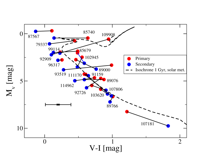
In Figure 2 we show a comparison of the values presented in Table 1. A few objects are clearly off from the expected 45 degrees sequence, we have no explanation for these differences. A fit of $V_{Sim}$ vs. $V_{Hip}$, excluding the two deviant points indicated in the plot (HIP 92909 and 11170) has an rms of 0.027 mag, while a fit of $V_{Sys}$ vs. $V_{Hip}$, excluding the three deviant points (HIP 85679, 85740, and 93519), has an rms of 0.058 mag, which we will take as an estimate of the uncertainty of the photometry in Section 4 (see also Figure 8). These values are approximately consistent with the color uncertainties reported in Table 1. Regarding the uncertainty of our $\Delta I$ values, this is more difficult to ascertain, since it depends on a number of factors such as the angular separation between the components, the quality of the night when the measurement was performed, the brightness of the primary, etc. From repeated measurements on different nights for several of our objects we have estimated an average uncertainty of $\sigma_{\Delta I}\sim 0.18$ mag, which we take as the typical error for $\Delta I$ for our sample of binaries. This value, being much larger than the estimated uncertainty of the $V$-band magnitudes, limits a finer analysis and interpretation of the location of the components of these systems in the H-R diagram (see Figure 8), as explained in Section 4.

Figure 2: Comparison of the photometric values presented in Table 1. We indicate the outlier objects (Hipparcos number) that exhibit a very large difference in the reported magnitudes. A linear fit between $V_{Sim}$ and $V_{Sys}$ vs. $V_{Hip}$ (excluding the outliers) gives the rms values indicated in the legend, this is an indication of the uncertainty of the photometry. The dotted line is not a fit, it only shows the expected one-to-one relationship.

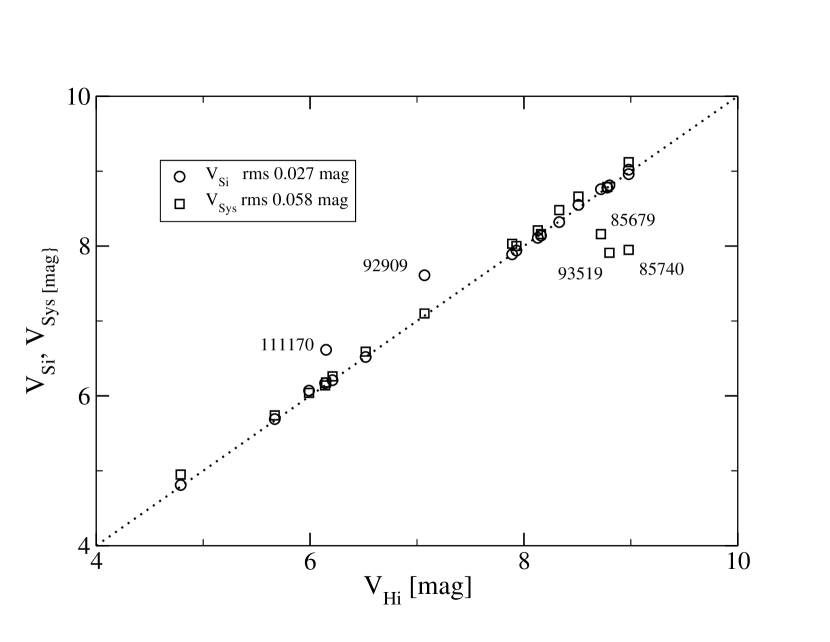
Two of the objects in Table 1 are double-lined spectroscopic binaries (SB2), namely HIP 89000 (YSC 132Aa,Ab), and HIP 111170 (CHR 111). For these, we retrieved their radial velocity measurements from the 9th Catalogue of Spectroscopic Binary Orbits (Pourbaix et al. (2004)). In Section 3.6 we perform a joint solution of the astrometric and radial velocity data of these two systems (see Table 5).

Regarding the astrometric calibration, precision, and accuracy of our astrometric data, the reader is referred to the publications from which these data were taken, and where these issues are extensively discussed. In a nutshell, HRCAM on SOAR routinely delivers precisions of 1-3 mas in angular separation for objects brighter than $V\sim 12$. In our survey, the magnitude difference of the resolved systems ranges from near-equal brightness components to $\Delta m\sim 6$ mag, while the range in separation goes from $\sim$35 mas (telescope diffraction limit in the $V$-band) to 2.0 arcsec (we have a few resolutions below the diffraction limit, down to 12 mas). For many systems we have also been able to uniquely resolve the quadrant ambiguity inherent to Speckle imaging from either a resolved long-exposure image, or from the shift-and-add (or “lucky”) images. In these latter cases, these quadrants are “enforced” in the orbital solution, which allows, in turn, quadrant resolutions of older data as well, by imposing self-consistency of the computed orbit (a process that, one must admit, is somewhat “subjective”).

3 Orbits

For our orbital calculations we have used a newly developed code to compute orbits, based on MCMC, whose implementation is described in the next subsections. The main motivation behind this approach is to exploit features that are inherent to these methods, namely (i) to provide confidence limits to the derived orbital elements, and (ii) to generate posterior probability density functions (PDF hereafter) for each orbital element, as well as for the derived masses. PDFs also allow us to explore the possible existence of non-unique solutions given the current data. An additional motivation has been the possibility to incorporate missing or partial data (e.g., only position angle $\theta$ but not separation $\rho$, or vice-versa), which might be particularly important if those data fall in a critical part of the orbit (e.g., see Claveria et al. (2016)). MCMC methods (see, e.g., Hestroffer (2012); Mede & Brandt (2014)) are currently widely used in exoplanet research (akin to a binary system), mostly for the interpretation of radial velocity data (Tuomi & Kotiranta (2009); Otor et al. (2016)), but also for astrometric orbits (see., e.g., Sahlmann et al. (2013)).

In the following subsections we present an outline of our specific MCMC implementation, and the main results as applied to the visual and spectroscopic binaries in the sample reported here.

3.1 Orbital adjustment through Eggen’s effect

Long ago, Eggen (1967), suggested that the $a^{3}/P^{2}$ quotient can often be well-determined even if the individual values of the semi-major axis $a$ and the period $P$ are not accurately known. Nowadays this is referred to as Eggen’s effect (Lucy (2014)). Thus, if the estimate of $P$ suffers a dramatic change after new observations are incorporated into the analysis, the corresponding estimate of parameter $a$ may undergo a shift on its value such that it compensates that variation, yielding a similar value for the $a^{3}/P^{2}$ ratio. Numerical results presented in Lucy (2014) strongly support this conjecture, as they suggest that, if the orbital coverage exceeds $40\%$ of the full orbit, a reasonable estimate of $a^{3}/P^{2}$ can, in general, be obtained. Of course, there are additional factors to take into account, such as the quality of the observations, the specific orbital section being covered (points near the periastron are significantly more informative than those that are far from it), and even the particular orbital configuration being observed –some orbits may be intrinsically more challenging to examine than others; think of cases with inclination ($i$) very close to $90^{\circ}$, for example.

As long as the observations provide a minimal orbital coverage of the object under study, the so-called Eggen’s effect opens up the possibility of estimating the mass by identifying the set of feasible orbital configurations, even if they involve a wide range of values for $a$ and $P$. The basic idea is that, rather than calculating the mass based on a single estimate, one can characterize mass (and its uncertainty) on the base of this set of feasible values.

Since our aim is not only to find a single feasible estimate for the orbital elements of the objects under study, but rather to characterize the uncertainty of its orbital parameters, in this paper we adopt a Bayesian approach for this problem. From a Bayesian standpoint, the set of feasible values mentioned in the previous paragraph takes the form of a posterior PDF. In this work, we construct the posterior PDF from a set of samples, which are drawn by means of the technique known as MCMC.

3.2 Model description

Assuming that phenomena such as mass transfer, relativistic effects, or even the presence of non visible additional bodies, do not affect the observed objects to a significant degree, we used a Keplerian model to describe the orbits of the analyzed binary stars. This model requires seven parameters (represented in what follows by the vector $\vec{\vartheta}$) to fully characterize the trajectory of a visual binary star (Equation 1), that is, to compute its ephemeris for any given epoch:

$$\vec{\vartheta}=\{P,T,e,a,\omega,\Omega,i\}$$ (1)

As to systems for which both astrometric and radial velocity measurements are available, one can perform a joint analysis by extending the parameter vector $\vec{\vartheta}$ presented in Equation (1) in the manner shown in Equation (2):

$$\vec{\vartheta}=\{P,T,e,a,\omega,\Omega,i,V_{CoM},\varpi,q\},$$ (2)

where $\{P,T,e,a,\omega,\Omega,i\}$ are the well-known Campbell elements and $V_{CoM}$, $\varpi$ and $q$ denote the velocity of the center of mass, the parallax of the system, and the mass ratio $m_{S}/m_{P}$ between the secondary of mass $m_{S}$ and the primary of mass $m_{p}$ respectively. The representation shown in Equation (2), and used previously, e.g., in Burgasser et al. (2015), has some distinct characteristics. First, it includes parallax $\varpi$ as one the parameters to be estimated rather than a value known in advance, thus putting into practice the somewhat unexplored possibility of utilizing combined data (i.e., astrometry and radial velocity) to estimate hypothesis-free parallaxes (Pourbaix (2000), Mason (2015)). Secondly, but as a consequence of including $\varpi$, it exploits all the restrictions imposed by the formulae of orbit position (Equations (A3), (A4)) and radial velocity (Equations (A6), (A7)), possibly leading to more precise inferences about the parameters. By contrast, in some codes, such as e.g., in ORBIT, the radial velocity amplitudes for the primary ($K_{P}$) and the secondary ($K_{S}$) (see Equations (A6) and (A7)) are taken as free parameters. Those methods have the advantage of not requiring a parallax value to perform the estimation, but omit the dependency of $K_{P}$ and $K_{S}$ on $a$, $i$ and $\omega$. Appendix A presents a summary of our actual implementation of the adopted Keplerian model, as well as the deduction of a novel mathematical formalism for a dimensionality reduction of the number of components of $\vec{\vartheta}$ for both visual and spectroscopic binaries, which we have applied in this work, further details on this will be given in a forthcoming paper. Our formulation makes it possible to explore a smaller number of parameters in each case: Three (instead of seven) for visual binaries, and seven (instead of ten) for spectroscopic binaries, while the remaining orbital parameters are unequivocally determined by a least-squares fit to the observed data.

3.3 Description of the Markov Chain Monte Carlo

MCMC designates a wide class of sampling techniques that rely on constructing a Markov Chain that explores the domain of the target PDF in such a way that it spends most of the time in areas of high probability (for an introduction to MCMC, the reader is referred to the tutorial by Andrieu et al. (2003)). MCMC provides a means to efficiently draw samples from distributions with complex analytic formulae and/or multidimensional domains. This subsection gives some basic details about the implementation of the MCMC used in this work. Orbital parameters of interest will be simply called “parameters”, whereas those related to the Markov Chain’s proposal distribution will be referred to as “algorithm-related parameters”.

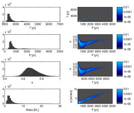
Our list consists of eighteen visual and two spectroscopic binary systems, with periods ranging from a few months (in the case of the spectroscopic binaries) to possibly thousands of years in the case of some visual binaries. Although a reparametrization of $T$ as $T^{\prime}=(T-T_{0})/P$ (an approach used in this work, and previously in Lucy (2014)), is useful to restrict the search range of the time of periastron passage to $[0,1)$, both the initial distribution and the search range of the period $P$ remains a difficult guess. The dimensionality reduction mentioned in Subsection 3.2 (and fully developed in Appendix A.1) alleviates to some extent the need of choosing an initial guess –for it suppresses parameters $a$, $\omega$, $\Omega$, $i$ from the analysis. However, the variability of the feasible ranges of $P$ among the studied objects imposes a diversity of scales among the posterior distributions. Moreover, the shape and orientation of each posterior PDF in the multi-dimensional feature space is unique (see a few examples in Figure 3, right panel). These factors make it difficult to choose a single set of algorithm-related parameters. At the same time, the list is long enough to make individual-case analysis undesirable.

In an effort to study the visual binaries under a single unified framework, rather than choosing algorithm-related parameters for each star separately –a task usually involving a lot of trial and error iterations–, we adopt the Differential Evolution MCMC approach presented by Braak (2006), called DE-MC hereinafter. DE-MC stems as the combination of a genetic algorithm called Differential Evolution (Storn & Price (1997)), described as “a simple and efficient heuristic for global optimization over continuous spaces” by its authors, and MCMC. The algorithm is based on the idea of running several Markov Chains in parallel but, instead of letting them run independently as in the classical MCMC convergence tests, it lets the chains learn from each other. This aims at dealing with the problem of choosing an appropriate scale and orientation for the proposal distribution.

The mutual learning between chains is accomplished by using a proposal distribution based on the DE “jumping step” considered in Storn & Price (1997). In that scheme, the proposal sample $\vartheta_{proposal}$ of each chain is obtained by adding to the previous sample ($\vartheta_{previous}$), the difference between the current values of two other randomly chosen chains (say $R1$, $R2$):

$$\vartheta_{proposal}=\vartheta_{previous}+\gamma\cdot(\vartheta_{R1}-\vartheta_{R2})+w,$$ (3)

where $\vartheta$ represents a point in the feature space, the coefficient $\gamma$ is a term that modulates the difference vector (its optimal value depends on the dimension of the feature space, $d$), and $w$ is an additional perturbation drawn from a distribution with unbounded support (e.g., a normal distribution) and small variance with respect to that of the target distribution (for further details, see Braak (2006)). The $w$ term is aimed at guaranteeing the irreducibility condition of MCMC and, in practice, this additional noise is useful to explore the feature space at the level of a small vicinity. The term $\gamma\cdot(\vartheta_{R1}-\vartheta_{R2})$, on the other hand, contributes to make larger leaps, without falling in zones of low likelihood. The algorithm is proven to meet the reversibility, aperiodicity, and irreducibility conditions which are required for MCMC in Braak (2006). The method is summarized in pseudo-code in Appendix C, Figure 10.

Since we are interested in characterizing a posterior distribution, a fitness function $f$ is defined as the posterior PDF, which has the canonical form of $prior\times likelihood$ (see, e.g., Gelman et al. (2013)). Terms from the prior PDF can be dropped, as uniform priors were used for the three relevant exploration parameters after dimensionality reduction, namely: $T^{\prime}$ (range $(0,1)$), $\log P$ (range ($\log 10$ yr, $\log 5000$ yr)) and $e$ (range $(0,0.99)$). Thus, the likelihood function can be directly used to compute the Metropolis-Hastings ratio Assuming independent individual Gaussian errors for each observation, the likelihood function for the $i$-th iteration with orbital parameters $\vartheta_{i}$ is defined as:

$$f(\vartheta_{i})\propto\displaystyle\exp\biggl{(}-\frac{1}{2}\Bigl{(}\sum_{k=1}^{N_{x}}\frac{1}{\sigma_{x}^{2}(k)}[X(k)-X^{model}(k,i)]^{2}+\sum_{k=1}^{N_{y}}\frac{1}{\sigma_{y}^{2}(k)}[Y(k)-Y^{model}(k,i)]^{2}\Bigr{)}\biggr{)},$$ (4)

where $(X(k),Y(k))$ is the k-th observation of the apparent orbit with uncertainties $(\sigma_{x}(k),\sigma_{y}(k))$, $(X^{model}(k,i),Y^{model}(k,i))$ are the computed ephemerides (which depend on $\vartheta_{i}$, see Appendix A), and where we have $N_{x}$ observations in $X$ and $N_{y}$ observations in $Y$ (usually $N_{x}=N_{y}$). Equation (4) results from the assumption that the residual of each data point follows an independent Gaussian distribution. Note that, as in any orbital calculation procedure, the weights assigned to each observational point play a critical role in the solution.

The algorithm-related parameters in this case are: the number of chains $N_{chains}$; the coefficient $\gamma$; the parameters of the distribution of $w$. Following the guidelines presented in Braak (2006), we fixed $N_{chains}=10$ (the recommendation is to choose $N_{chains}>2\cdot d$), $\gamma=2.38/\sqrt{2\cdot d}$. Values for $w$ are drawn from $\mathcal{N}(0,\Sigma)$, where $\Sigma$ is a diagonal matrix with: $\sigma^{2}_{T^{\prime}}=0.01$, $\sigma^{2}_{\log P}=0.01\cdot(\log P_{upper}-\log P_{lower})$ and $\sigma^{2}_{e}=0.01$. To obtain the final posterior distribution, we ran DE-MC with $N_{steps}=10^{6}$ for each object, discarding the first $10^{5}$ samples of each chain (the so-called “burn-in period”). As shown in Braak (2006), each chain distributes as the target distribution, so that the set of all chains can be treated as a single collection of samples, once the burn-in period is dropped. Therefore, with our adopted parameters, this results in a single-chain of $9\times 10^{6}$ samples.

This is a minimalist description of the algorithm since further details on the inner working of our MCMC implementation, full tests, and other applications of the method will be given in a separate publication. We can however mention that our code has been extensively tested against simulated and real data, and its results have also been compared to other codes, including the IDL-driven interactive ORBIT code developed by Tokovinin (1992) which employs a $\chi^{2}$ minimization approach through a Levenberg-Marquardt parameter exploration method to determine the Campbell orbital elements by a fit to the data (see Appendix B.2), and a code that uses minimization through a downhill simplex algorithm, developed by MacKnight & Horch (2004), and used extensively by Horch and collaborators (see., e.g., Horch et al. (2015)).

3.4 Orbital elements for our Visual Binaries

The results of our MCMC code, described in the previous subsection, when applied to the eighteen visual binaries of the sample presented in Section 2 are shown in Table 2. For each object, two sets of numbers for the orbital elements are provided: The upper row represents the configuration with the smallest mean square sum of the O-C overall residuals , while the lower row shows the median derived from the posterior PDF of the MCMC simulations, as well as the upper (third) quartile ($Q75$) and lower (first) quartile ($Q25$) of the distribution in the form of a superscript and subscript respectively. The orbital coverage, and the reliability of the fitted orbital parameters, ranges from what one could consider as almost “final” orbits (e.g., HIP 85679, HIP 92909, HIP 102945, HIP103620, HIP 109908) to those with very poor coverage and uncertain orbits (e.g., HIP 85740, TYC 1566-1708-1, HIP 89766). In the penultimate column we give an indication of the “Grade” of the orbit as defined in the WDS, while the last column has the reference for the latest orbit published for each object (or “New” if none was available). The reason why ML/MAP is preferred over the expected value is that, for most of the cases studied in this work, the PDFs are rather disperse and asymmetrical, thus yielding average values that are not in good agreement with the observations. The only exceptions are those orbits with good orbital coverage: HIP 85679, HIP 102945, and HIP 103620 (to mention a few examples), for which the expected value approximately coincides with the MAP/ML estimate.

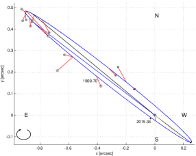
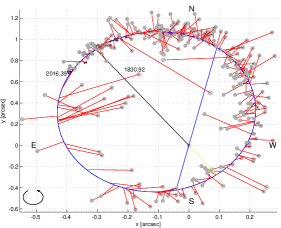
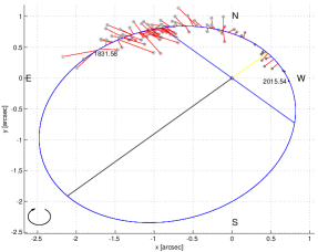
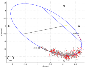
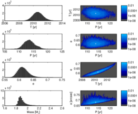
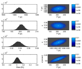
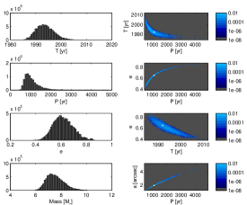
In Figure 3 we show some examples of orbital solutions and PDFs for objects in our sample. By looking at Table 2 and Figure  3 we can say that, in general, well determined orbits show a ML value that approximately coincides with the 2nd quartile of the PDF, the inter-quartile range is relatively well constrained, and the PDFs show a Gaussian-like distribution, meanwhile poor orbits show PDFs with very long tails (and therefore large inter-quartile ranges) on which the ML value usually exceeds by much the 2nd quartile, and the PDFs are tangled.

Table 2: Orbital elements of our visual binaries

HIP	P	T0	e	a	$\omega$	$\Omega$	i	Gr	Orbit
	(yr)	(yr)		($\arcsec$)	(∘)	(∘)	(∘)	Current $\rightarrow$ New	reference
79337	60.60	2000	0.049	0.1280	93	83.36	91.13	3$\rightarrow$3	Doc2013d
	${59.31}_{-0.68}^{+0.91}$	${1994}_{-27}^{+6}$	${0.016}_{-0.009}^{+0.024}$	${0.1285}_{-0.0003}^{+0.0002}$	${121}_{-31}^{+115}$	${83.35}_{-0.01}^{+0.01}$	${91.11}_{-0.01}^{+0.01}$
85679	202	1986.53	0.506	0.286	238.6	166.8	151.7	5$\rightarrow$3	USN2002
	${201}_{-12}^{+14}$	${1986.46}_{-0.45}^{+0.44}$	${0.503}_{-0.028}^{+0.027}$	${0.286}_{-0.008}^{+0.008}$	${237.5}_{-6.5}^{+5.6}$	${165.8}_{-5.2}^{+4.4}$	${150.9}_{-2.8}^{+3.0}$
85740	2302	1988	0.87	1.317	7	59	109.3	5$\rightarrow$4	Cou1999b
	${136}_{-31}^{+47}$	${2025}_{-42}^{+24}$	${0.26}_{-0.14}^{+0.17}$	${0.191}_{-0.018}^{+0.050}$	$9_{-34}^{+47}$	$64_{-163}^{+4}$	${116.8}_{-4.1}^{+3.9}$
87567	895	1961.74	0.750	0.641	300.3	36.7	36.3	5$\rightarrow$4	Doc1991b
	${753}_{-154}^{+251}$	${1961.52}_{-0.77}^{+0.73}$	${0.718}_{-0.049}^{+0.051}$	${0.571}_{-0.080}^{+0.123}$	${296.0}_{-7.8}^{+6.9}$	${40.4}_{-6.0}^{+6.6}$	${36.1}_{-1.8}^{+1.8}$
1566-1708-1	3431	1976.6	0.84	3.31	219	153.3	125.8	5$\rightarrow$5	USN2002
	${497}_{-150}^{+294}$	${1978.1}_{-2.7}^{+3.4}$	${0.41}_{-0.18}^{+0.17}$	${0.98}_{-0.17}^{+0.31}$	${233}_{-7}^{+10}$	${166.0}_{-5.1}^{+5.2}$	${124.1}_{-2.0}^{+1.9}$
89076	427	1977	0.43	0.432	7	134	41.9	5$\rightarrow$4	USN2002
	${229}_{-36}^{+64}$	${1990}_{-31}^{+63}$	${0.21}_{-0.11}^{+0.15}$	${0.311}_{-0.032}^{+0.058}$	$5_{-33}^{+51}$	$98_{-187}^{+16}$	${43.4}_{-8.3}^{+8.4}$
89766	1119	2000	0.609	3.05	114	119.38	84.81	X$\rightarrow$5	NEW
	${309}_{-78}^{+114}$	${2049}_{-15}^{+9}$	${0.383}_{-0.091}^{+0.176}$	${1.96}_{-0.13}^{+0.27}$	${209}_{-50}^{+33}$	${119.44}_{-0.15}^{+0.16}$	${86.73}_{-0.63}^{+0.79}$
91159	532	2364	0.709	2.80	96	34.3	110.1	4$\rightarrow$4	Hei1995
	${595}_{-99}^{+189}$	${2380}_{-90}^{+129}$	${0.686}_{-0.044}^{+0.053}$	${2.94}_{-0.17}^{+0.29}$	${100}_{-6}^{+12}$	${32.2}_{-4.0}^{+3.7}$	${110.5}_{-1.2}^{+1.1}$
92726	764	1914.7	0.746	1.20	342	30	35.3	5$\rightarrow$4	Hei1998
	${549}_{-135}^{+249}$	${1911.6}_{-3.7}^{+3.4}$	${0.702}_{-0.042}^{+0.051}$	${1.03}_{-0.10}^{+0.21}$	${338}_{-8}^{+11}$	${17}_{-8}^{+11}$	${42.9}_{-6.9}^{+6.5}$
92909	154.7	2008.2	0.221	0.295	63	80.1	129.3	3$\rightarrow$3	Doc1988c
	${154.2}_{-8.7}^{+10.7}$	${2008.3}_{-2.8}^{+3.0}$	${0.222}_{-0.021}^{+0.026}$	${0.295}_{-0.014}^{+0.015}$	${63}_{-10}^{+11}$	${80.2}_{-1.1}^{+1.1}$	${129.3}_{-1.8}^{+1.8}$
93519	1123	1992.1	0.647	1.97	95	48	151.3	5$\rightarrow$5	Alz1998a
	${975}_{-168}^{+263}$	${1993.5}_{-2.3}^{+2.5}$	${0.612}_{-0.050}^{+0.056}$	${1.82}_{-0.18}^{+0.27}$	${97}_{-14}^{+10}$	${49}_{-10}^{+6}$	${149.0}_{-2.6}^{+2.5}$
96317	2651	1993	0.83	1.384	195	76.9	70.7	3$\rightarrow$3	Ole1994
	${279}_{-56}^{+126}$	${2015}_{-14}^{+14}$	${0.33}_{-0.10}^{+0.12}$	${0.294}_{-0.044}^{+0.089}$	${234}_{-25}^{+37}$	${77.9}_{-4.3}^{+4.6}$	${62.8}_{-3.2}^{+3.1}$
99114	52	2017.3	0.265	0.166	159	66	22.4	X$\rightarrow$4	NEW
	${155}_{-19}^{+28}$	${2016.8}_{-7.2}^{+5.8}$	${0.294}_{-0.043}^{+0.053}$	${0.175}_{-0.008}^{+0.013}$	${154}_{-78}^{+40}$	${77}_{-19}^{+35}$	${32.6}_{-6.6}^{+6.4}$
102945	200.7	1896.8	0.535	0.816	45.8	174.32	64.06	2$\rightarrow$2	RAO2015
	${200.7}_{-1.1}^{+1.1}$	${1896.8}_{-0.40}^{+0.39}$	${0.535}_{-0.005}^{+0.006}$	${0.816}_{-0.006}^{+0.006}$	${45.9}_{-1.2}^{+1.2}$	${174.31}_{-0.39}^{+0.38}$	${64.06}_{-0.27}^{+0.26}$
103620	113.7	2010.54	0.611	0.682	207.2	63.07	93.69	X$\rightarrow$3	NEW
	${113.6}_{-1.2}^{+1.3}$	${2010.62}_{-0.46}^{+0.48}$	${0.613}_{-0.011}^{+0.012}$	${0.684}_{-0.006}^{+0.007}$	${207.6}_{-2.6}^{+2.8}$	${63.02}_{-0.31}^{+0.31}$	${93.66}_{-0.19}^{+0.16}$
107806	32.8	2014.1	0.158	0.224	98	127.22	87.84	X$\rightarrow$4	NEW
	${32.9}_{-2.2}^{+2.9}$	${2013.9}_{-1.6}^{+1.2}$	${0.164}_{-0.021}^{+0.021}$	${0.226}_{-0.011}^{+0.015}$	${97}_{-22}^{+20}$	${127.23}_{-0.09}^{+0.10}$	${87.88}_{-0.12}^{+0.14}$
109908	19.09	1996.39	0.562	0.169	92.5	105.0	65.70	3$\rightarrow$3	Tok2015c
	${19.04}_{-0.18}^{+0.16}$	${1996.35}_{-0.18}^{+0.17}$	${0.561}_{-0.020}^{+0.025}$	${0.168}_{-0.002}^{+0.003}$	${92.61}_{-0.54}^{+0.67}$	${104.2}_{-1.8}^{+1.6}$	${65.69}_{-0.53}^{+0.44}$
114962	381	1927.8	0.470	0.942	92.1	44.25	86.89	4$\rightarrow$3	Hei1991
	${388}_{-24}^{+34}$	${1928.6}_{-1.5}^{+2.1}$	${0.464}_{-0.041}^{+0.040}$	${0.957}_{-0.041}^{+0.053}$	${93.7}_{-4.3}^{+6.2}$	${44.34}_{-0.20}^{+0.21}$	${86.93}_{-0.06}^{+0.07}$

Figure 3: Examples of orbital solutions (left panel) and PDFs (right panel), from top to bottom: HIP 103620, HIP 102945, HIP 93519, and HIP 91159. HIP 103620 and HIP 102945 have well defined orbits and tight (usually Gaussian-like) PDFs. HIP 93519, and HIP 91159 represent two typical examples of objects with incomplete orbital coverage, and tangled PDFs. See Section 4 for further comments on individual objects. On the orbits we indicate the first and last epoch of observation. Larger and lighter-grey points have less weight in the solution than smaller darker points.

3.5 Mass sums and dynamical parallaxes

The orbital parameters and their uncertainties presented in the previous subsection allow us to compute mass sums for those objects that have a published trigonometric parallax. In Table 3 we indicate, for each of our visual binaries, their spectral type from the literature (second column), trigonometric parallax (third column, on the second line of that column we show the parallax uncertainty) and the astrometric mass sum (in solar masses, last column of the table) obtained from the published parallax and the period and semi-major axis from Table 2. For each object, in the upper line we indicate the mass sum from the maximum likelihood (ML) solution, while in the second line we report the second quartile (median), with the first quartile as a subscript and the third quartile as a superscript. The quartiles reported for the mass sum comes from the MCMC orbital results alone, i.e., they do not include the error in the trigonometric parallax.

As a test of the reliability of our orbits, we have also computed dynamical parallaxes (fourth column), primary (fifth column), secondary (sixth column), and total (seventh column) dynamical masses on Table 3. To compute all these values we have adopted the photometry values for the primary ($V_{P}$) and secondary ($V_{S}$) from Table 1, the values of $P$ and $a$ from Table 2, and the MLR for main sequence stars from Henry & McCarthy (1993), who provide an easy-to-evaluate mass vs. $M_{V}$ polynomial relationship for objects below 1$M_{\odot}$. A few objects in our list are not on the main sequence, for them, of course, the adopted MLR relationship (and therefore, the implied dynamical parallax) is not valid, the most striking case being HIP 109908 which is further discussed in Section 4 (see also Figure 8). The quoted uncertainty values for the dynamical parallax come exclusively from the range of solutions of our MCMC simulations, and not from uncertainties on either the photometry or the width of the MLR relationship.

Table 3: Trigonometric and dynamical parallaxes (visual binaries).

HIP	Sp. Type	Trig. Parallax	Dyn. parallax	Mass${}^{\mbox{\tiny{dyn}}}_{\mbox{\tiny{P}}}$	Mass${}^{\mbox{\tiny{dyn}}}_{\mbox{\tiny{S}}}$	Mass${}^{\mbox{\tiny{dyn}}}_{\mbox{\tiny{T}}}$	Mass${}_{\mbox{\tiny{T}}}$
		(mas)	(mas)	($\it{M}_{\odot}$)	($\it{M}_{\odot}$)	($\it{M}_{\odot}$)	($\it{M}_{\odot}$)
79337	F0IV	5.13	5.02	2.35	2.19	4.53	4.24
		$\pm 0.70$	${5.13}_{-0.07}^{+0.05}$	${2.32}_{-0.01}^{+0.01}$	${2.16}_{-0.01}^{+0.01}$	${4.49}_{-0.02}^{+0.03}$	${4.48}_{-0.15}^{+0.10}$
85679	F0V	5.06	5.72	1.69	1.37	3.05	4.41
		$\pm 0.97$	${5.74}_{-0.10}^{+0.11}$	${1.68}_{-0.01}^{+0.01}$	${1.36}_{-0.01}^{+0.01}$	${3.05}_{-0.02}^{+0.02}$	${4.45}_{-0.20}^{+0.22}$
85740	A5	2.24	5.00	1.72	1.72	3.44	38
		$\pm 1.32$	${4.91}_{-0.38}^{+0.56}$	${1.73}_{-0.08}^{+0.06}$	${1.73}_{-0.08}^{+0.06}$	${3.46}_{-0.16}^{+0.12}$	${37}_{-7}^{+12}$
87567	B3/5III	3.68	3.87	2.86	2.82	5.68	6.61
		$\pm 0.54$	${3.89}_{-0.04}^{+0.05}$	${2.85}_{-0.02}^{+0.02}$	${2.81}_{-0.02}^{+0.02}$	${5.67}_{-0.03}^{+0.03}$	${6.67}_{-0.19}^{+0.20}$
1566$-$1708$-$1	G0	$-$	11.49	1.18	0.85	2.03	$-$
		$-$	${12.46}_{-0.53}^{+0.74}$	${1.14}_{-0.02}^{+0.02}$	${0.83}_{-0.02}^{+0.01}$	${1.97}_{-0.04}^{+0.03}$	$-$
89076	G3V	9.88	5.51	1.32	1.32	2.64	0.46
		$\pm 1.43$	${5.90}_{-0.36}^{+0.64}$	${1.28}_{-0.05}^{+0.03}$	${1.28}_{-0.05}^{+0.03}$	${2.57}_{-0.10}^{+0.06}$	${0.55}_{-0.08}^{+0.17}$
89766	K3+Vk	31.35	24	0.87	0.80	1.66	0.7
		$\pm 1.25$	${35}_{-5}^{+10}$	${0.77}_{-0.06}^{+0.04}$	${0.71}_{-0.05}^{+0.03}$	${1.47}_{-0.11}^{+0.07}$	${2.1}_{-0.7}^{+2.1}$
91159	G2V	29.63	32.8	1.12	1.09	2.21	2.99
		$\pm 0.83$	${30.5}_{-3.1}^{+3.8}$	${1.15}_{-0.05}^{+0.05}$	${1.12}_{-0.05}^{+0.05}$	${2.27}_{-0.10}^{+0.09}$	${2.47}_{-0.60}^{+0.89}$
92726	G5V	12.99	11.2	1.14	0.96	2.10	1.36
		$\pm 1.65$	${12.2}_{-1.0}^{+1.2}$	${1.10}_{-0.04}^{+0.04}$	${0.94}_{-0.03}^{+0.03}$	${2.04}_{-0.07}^{+0.06}$	${1.67}_{-0.33}^{+0.49}$
92909	A3IV	6.99	6.70	1.84	1.74	3.58	3.15
		$\pm 0.83$	${6.69}_{-0.09}^{+0.10}$	${1.84}_{-0.01}^{+0.01}$	${1.74}_{-0.01}^{+0.01}$	${3.58}_{-0.02}^{+0.02}$	${3.14}_{-0.11}^{+0.12}$
93519	G3/5V	9.48	13.86	1.19	1.09	2.28	7.14
		$\pm 0.25$	${14.11}_{-0.31}^{+0.36}$	${1.18}_{-0.01}^{+0.01}$	${1.09}_{-0.01}^{+0.01}$	${2.27}_{-0.02}^{+0.02}$	${7.47}_{-0.43}^{+0.51}$
96317	A0	6.42	4.77	1.74	1.73	3.47	1.43
		$\pm 1.33$	${4.51}_{-0.14}^{+0.16}$	${1.79}_{-0.03}^{+0.02}$	${1.77}_{-0.03}^{+0.03}$	${3.56}_{-0.05}^{+0.05}$	${1.23}_{-0.09}^{+0.11}$
99114	F2IV	3.90	3.77	1.87	1.82	3.69	3.34
		$\pm 0.65$	${3.90}_{-0.14}^{+0.25}$	${1.84}_{-0.05}^{+0.03}$	${1.79}_{-0.05}^{+0.03}$	${3.64}_{-0.10}^{+0.06}$	${3.63}_{-0.33}^{+0.63}$
102945	F6V	16.47	16.59	1.62	1.33	2.95	3.02
		$\pm 0.59$	${16.59}_{-0.09}^{+0.09}$	${1.618}_{-0.004}^{+0.004}$	${1.331}_{-0.003}^{+0.003}$	${2.95}_{-0.01}^{+0.01}$	${3.02}_{-0.04}^{+0.04}$
103620	K0Vq	23.56	24.34	0.88	0.82	1.70	1.88
		$\pm 0.31$	${24.39}_{-0.13}^{+0.22}$	${0.883}_{-0.003}^{+0.002}$	${0.818}_{-0.002}^{+0.001}$	${1.701}_{-0.005}^{+0.003}$	${1.89}_{-0.03}^{+0.04}$
107806	G6V	24.09	17.18	1.08	0.99	2.06	0.75
		$\pm 1.03$	${17.35}_{-0.22}^{+0.25}$	${1.07}_{-0.01}^{+0.01}$	${0.98}_{-0.01}^{+0.01}$	${2.06}_{-0.01}^{+0.01}$	${0.77}_{-0.03}^{+0.03}$
109908	G8III+G	11.87	15.22	2.14	1.59	3.73	7.88
		$\pm 0.43$	${15.20}_{-0.26}^{+0.22}$	${2.15}_{-0.01}^{+0.02}$	${1.59}_{-0.01}^{+0.01}$	${3.74}_{-0.02}^{+0.03}$	${7.84}_{-0.34}^{+0.30}$
114962	F(8)w	15.08	13.80	1.13	1.07	2.19	1.68
		$\pm 1.80$	${13.80}_{-0.14}^{+0.15}$	${1.126}_{-0.005}^{+0.004}$	${1.068}_{-0.004}^{+0.004}$	${2.19}_{-0.01}^{+0.01}$	${1.68}_{-0.04}^{+0.05}$

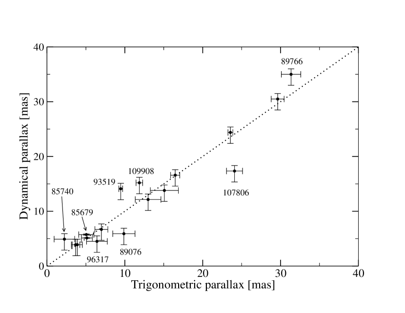
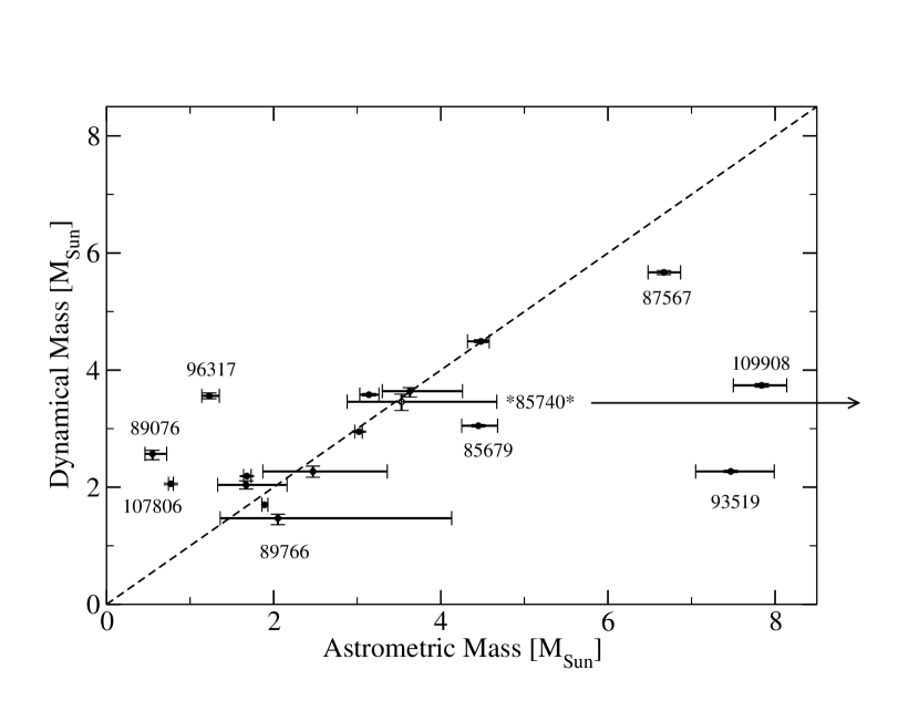
In Figures 4 and 5 we show the values of Table 3 in graphical form. Generally speaking, there is good agreement between the dynamical and astrometric parallaxes and masses, with some notable exceptions that can be attributed to either a poor orbit determination, a large parallax uncertainty, poor photometry, or a combination of these. This is discussed on an object-by-object basis in more detail in Section 4.

We note that, given the relatively small distances for all our targets, our dynamical parallaxes have been calculated assuming no interstellar absorption. Using the reddening model by Mendez & van Altena (1998), we can demonstrate that this is indeed a reasonable assumption: If we take the last point plotted in Figure 4 (HIP 89766, at a distance of about 32 pc, see Table 3), the model predicts an extinction in the V-band of 0.027 mag at that Galactic location. With that extinction, the ML and median dynamical parallaxes do not change with respect to the values given in Table 3. For the smallest parallax object in our whole sample, HIP 85740, with a distance of  446 pc, the Mendez & van Altena (1998) model predicts 0.181 mag of extinction, and the corresponding ML and median dynamical parallaxes change from 5.00, 4.91 mas (no extinction) to 4.93, 4.84 mas (extincted) respectively, i.e., completely within the computed inter-quartile range reported in Table 3. Finally, according to the Mendez & van Altena (1998) reddening model, our most-extincted target is the third more distant of our list, namely, HIP 87567, at a distance of only 272 pc, but located towards the Galactic center ($(l,b)=(355\arcdeg.9,-4\arcdeg.4)$), with $A_{V}=0.4$ mag. In this case, the corresponding ML and median dynamical parallaxes change from 3.87, 3.89 mas (no extinction) to 3.73, 3.75 mas (extincted) respectively, a difference of only 0.14 mas (almost four times smaller than the quoted uncertainty for the trigonometric parallax of this target), and within $2\sigma$ of the inter-quartile range. For all other targets in our list, interstellar absorption effects can be safely ignored in the calculation of the dynamical parallaxes.

Figure 4: Comparison of the dynamical vs. trigonometric parallaxes from the values presented in Table 3. We indicate the objects (Hipparcos number) that exhibit a very large difference between the dynamical and astrometric values, or those that appear as discrepant in Figure 5. The dotted line is not a fit, it only shows the expected one-to-one relationship in both panels. In the ordinate, the quantity shown is the $2^{nd}$ quartile from Table 3.

Figure 5: Comparison of the dynamical vs. astrometric mass sums from the values presented in Table 3. We indicate the objects (Hipparcos number) that exhibit a very large difference between the dynamical and astrometric values. The dotted line is not a fit, it only shows the expected one-to-one relationship in both panels. In both axes the quantity shown is the $2^{nd}$ quartile from Table 3. HIP 85740 falls out of scale to the right in the abscissa in this plot, and it is indicated as an arrow at the level of its dynamical mass (this object is further discussed in Section 4). If we assume instead the trigonometric parallax value indicated in Section 4 for HIP 85740, it falls in this plot as indicated by its HIP number between asterisks.

3.6 Spectroscopic binaries

As mentioned in Section 2, two of our speckle targets turned out to be SB2, HIP 89000, and HIP 111170. A combined solution for the astrometric data, plus radial velocity data was performed using our MCMC code.

The spectroscopic binaries were analyzed by means of the more traditional Gibbs sampler introduced by Geman & Geman (1984), instead of the DE-MC approach explained in Section 3.3. A number of practical reasons support this decision: first, as the dimensionality of the feature space is larger than that of the visual binary problem – ten dimensions, or seven dimensions with the dimensionality reduction (see Appendix A.1) –, a larger number of chains must be run within the DE-MC algorithm (at least two times the size of the feature space, and preferably more), increasing the computational costs too much; secondly, unlike the visual binaries in our sample, a tighter exploration range for the period can be proposed from a simple visual inspection of the observations. Finally, although a raw Metropolis-Hastings MCMC would be a simpler approach, the dimension of the problem is large enough, and the location of the solutions concentrated enough (see Figure 7), making it highly probable to fall in zones of low likelihood after a multidimensional random jump is applied on a sample, possibly reaching pathologically low values of acceptance probability.

The Gibbs sampler relies on sequentially sampling each component of the feature space according to the conditional distributions. On the long run, this scheme is equivalent to draw samples from the joint posterior distribution. Although the pseudo-code (Appendix C, Figure 11) shows each component being sampled individually, components can also be grouped in blocks if it has some advantage (for example, if a sub-set of the parameter vector has a known and easy-to-sample distribution). As the conditional posteriors do not have a standard form in this problem, we used a Metropolis-within-Gibbs approach, that is, generating a new sample according to a proposal distribution (modifying one component or block of components of the parameter vector at once), and rejecting or accepting it according to the Metropolis-Hastings ratio. The Gibbs sampler has been used in the past in the study of exoplanet orbits, see e.g. Ford (2005).

Under the assumption that individual errors of both astrometric and radial velocity sources are Gaussian, in this case the likelihood function has the following form (compare to Equation (4)):

$$f(\vartheta_{i})\propto\displaystyle\exp\biggl{(}-\frac{1}{2} \Bigl{(}\sum_{k=1}^{N_{x}}\frac{1}{\sigma_{x}^{2}(k)}[X(k)-X^{model}(k,i)]^{2}+\sum_{k=1}^{N_{y}}\frac{1}{\sigma_{y}^{2}(k)}[Y(k)-Y^{model}(k,i)]^{2}+$$

$$\sum_{k=1}^{N_{VP}}\frac{1}{\sigma_{p}^{2}(k)}[V_{P}(k)-V_{P}^{model}(k,i)]^{2}+\sum_{k=1}^{N_{VS}}\frac{1}{\sigma_{S}^{2}(k)}[V_{S}(k)-V_{S}^{model}(k,i)]^{2}\Bigr{)}\biggr{)},$$

where $(V_{P}(k),V_{S}(k))$ are the primary (with $N_{VP}$ measurements) and secondary (with $N_{VS}$ measurements) Heliocentric radial velocity observations with uncertainties $(\sigma_{P}(k),\sigma_{S}(k))$ respectively, $(V_{P}^{model}(k,i),V_{S}^{model}(k,i))$ are the model radial velocities, and the remaining parameters have been defined earlier. This $f_{i}$ is used to calculate the ratios within the Metropolis-Hastings steps. We choose $N_{steps}=2\times 10^{6}$, with burn-in periods of $2\times 10^{5}$ for both HIP 89000 and HIP 111170. On each Metropolis-Hastings step, an additive Gaussian “noise” was used to propose new samples. Parameters of the proposal distributions, as well as the boundaries of the initial uniform distributions used for these two objects are shown in Table 4.

Table 4: Algorithm-related parameters for our two SB2 and astrometric binaries HIP 89000 and HIP 111170.

HIP	Alg-related	$P\tablenotemark{a}$	$T^{\prime}$	$e$	$\Omega$	$i$	$\varpi$	$q$
	parameters	$(yr)$			$(^{\circ})$	$(^{\circ})$	$(mas)$
89000	$\sigma\tablenotemark{b}$	$0.01$	$0.01$	$0.01$	$1$	$1$	$1$	$0.01$
	Range	$(0.1,1.0)$	$(0,1)$	$(0,0.99)$	$(0,360)$	$(0,180)$	$-$	$(0,1)$
111170	$\sigma\tablenotemark{b}$	$0.05$	$0.01$	$0.01$	$1$	$1$	$1$	$0.01$
	Range	$(0.2,3.0)$	$(0,1)$	$(0,0.99)$	$(0,360)$	$(0,180)$	$(32.35,46.35)$	$(0,1)$

In the case of HIP 89000, a Gaussian prior for the parallax was included in the fitness function $f$, since infeasible values of $\varpi$ were explored if the parallax was set free (this simply means that the available data is not yet informative enough to give an estimate for this parameter). For HIP 111170, instead, $\varpi$ is uniformly sampled in the wide range indicated in Table 4, and it converges to a value close to the dynamical parallax and not far from the trigonometric published parallax.

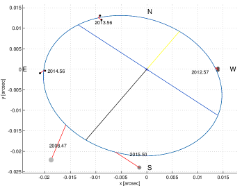
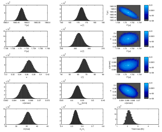
The resultant orbital elements, as well as the mass ratio and mass sum (with their derived uncertainties) are shown in Table 5. Since the posterior PDFs obtained here are tighter and more Gaussian-like than those obtained for our visual binaries, the expected value offers a good estimate of the target parameter vector, and is the estimator of choice in this section. In Figure 6 we show the joint fit to the orbit and the radial velocity curves. As it can bee seen from the table and figure, even in the case of a rather poor coverage of the astrometric orbit as is the case HIP 89000, the combined solutions produce very precise orbital parameters. This point is also highlighted in Figure 7, where we present the posterior PDFs, which exhibit tight and well-constrained distributions. In particular, judging from the quartile ranges, we can see that for HIP 89000 the mass ratio is determined with a 0.3% uncertainty, while the uncertainty on the mass sum is 8%. For HIP 111170 these value are 3% and 7% respectively.

Table 5: Orbital elements for our two SB2 and astrometric binaries HIP 89000 and HIP 111170.

HIP	P	T0	e	a	$\omega$	$\Omega$	i	$V_{CoM}$	$m_{S}/m_{P}$	$\varpi$	$m_{P}+m_{S}$
	(yr)	(yr)		($\arcsec$)	(∘)	(∘)	(∘)	($km~{}s^{-1}$)		(mas)	($\it{M}_{\odot}$)
89000	$0.54643$	$1990.675$	$0.302$	$0.0190$	$86.65$	$51.2$	$146.2$	$-14.131$	$0.956$	$21.31$	$2.52$
	${0.54643}_{-0.00006}^{+0.00006}$	${1990.675}_{-0.001}^{+0.001}$	${0.302}_{-0.002}^{+0.002}$	${0.0190}_{-0.0004}^{+0.0006}$	${86.65}_{-0.27}^{+0.27}$	${51.2}_{-2.4}^{+2.4}$	${146.3}_{-1.3}^{+1.2}$	$-14.131_{-0.008}^{+0.007}$	${0.956}_{-0.002}^{+0.003}$	${21.31}_{-0.21}^{+0.21}$	${2.54}_{-0.23}^{+0.25}$
111170	$1.7309$	$1965.48$	$0.367$	$0.0663$	$172.1$	$261.39$	$67.1$	$-9.573$	$0.538$	$35.5$	$2.17$
	${1.7309}_{-0.0006}^{+0.0006}$	${1965.47}_{-0.01}^{+0.01}$	${0.367}_{-0.007}^{+0.007}$	${0.0664}_{-0.0006}^{+0.0006}$	${172.1}_{-1.2}^{+1.2}$	${261.34}_{-0.90}^{+0.94}$	${67.2}_{-2.7}^{+2.7}$	$-9.574_{-0.010}^{+0.010}$	${0.537}_{-0.015}^{+0.016}$	${35.6}_{-1.1}^{+1.1}$	${2.17}_{-0.16}^{+0.18}$

Figure 6: MCMC fits to HIP 89000 (upper panel) and HIP 111170 (lower panel). The left panel shows the astrometric data and its fit, the right panel shows the fit to the radial velocity for both components.

 

Figure 7: Posterior distributions for spectroscopic binaries: HIP 89000 (top five rows), HIP 111170 (bottom five rows).

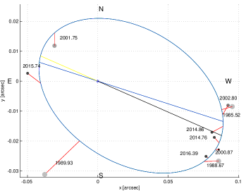
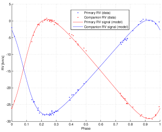
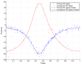
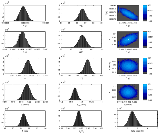
In Table 6 we present a comparison of the masses for the system as well as the individual component masses obtained from the joint fit of the orbit to the astrometric and radial velocity data shown in Table 5. The format of the table is similar to that of Table 3 in that it includes, for comparison purposes, dynamical parallaxes (fourth column) and individual and total dynamical masses (fifth to seventh columns) calculated in the same fashion as described in Section 3.5 for the visual binaries. The eighth column gives the total mass using the orbital elements given in Table 5, but adopting the published trigonometric parallax given in the third column of the table, whereas the ninth to eleventh columns gives the individual masses and the total mass, letting the parallax of the system be a free parameter of the MCMC code (i.e., adopting instead the parallax given in the twelfth column of Table 5). We note that the quartiles on Mass${}_{\mbox{\tiny{T}}}$ in Table 6 do not include any contribution from trigonometric parallax errors (just as in Table 3), while Mass${}^{\mbox{\tiny{comb}}}_{\mbox{\tiny{P}}}$, Mass${}^{\mbox{\tiny{comb}}}_{\mbox{\tiny{S}}}$, and Mass${}^{\mbox{\tiny{comb}}}_{\mbox{\tiny{T}}}$, being derived from MCMC simulations that have the parallax as a free parameter, do include the extra variance from this parameter.

In the case of HIP 89000 the agreement between all estimates of the mass is excellent as well as between the dynamical and published parallax. A preliminary astrometric orbit was published by Horch et al. (2015), and our combined orbital parameters agree quite well with theirs. We note that our SOAR data on 2008.47 and 2015.50 (see Figure 6) are uncomfortably discrepant, probably due to the small separation (below our diffraction limit), and which might require further observations on an 8m class telescope. For HIP 111170 the dynamical and orbital parallaxes ($\sim 36$ mas) agree quite well with each other, but are smaller by about 5 mas with respect to the published ($39.35\pm 0.70$ mas) trigonometric parallax (or more than $5\sigma$ of the published parallax uncertainty), thus leading to a larger total mass than that obtained by adopting the published parallax directly, as it can be readily seen in Table 6. This discrepancy could be due either to the rather poor coverage of the astrometric orbit (in comparison with the radial velocity curves), or to a biased Hipparcos parallax due to the orbital motion of the system, as shown by Söderhjelm (1999) (see, in particular his Section 3.1, and Table 2). We also note that the published photometry on SIMBAD for this object does not agree very well with that in the Hipparcos catalogue (see Figure 2), but there is very good agreement between $V_{Hip}$ and $V_{Sys}$ (see Table 1). We note that Pourbaix & Lampens (1999) performed a detailed comparison of Hipparcos trigonometric parallaxes with orbital parallaxes from the SB2s available at that time and found, in general, good correspondence between them with a few discrepant cases but at a less than $3\sigma$ level. The more precise Gaia parallaxes will probably shed some light into this issue.

As it can be seen from Table 6, the mass of the individual components for both binaries are determined with a formal uncertainty of $\sim 0.1M_{\odot}$, but this could possibly be improved by further speckle observations on an 8 m class telescope by providing a better-constrained astrometric orbit.

We finally note the good agreement for the triad ($V_{CoM}$, $K_{P}$, $K_{S}$) reported by the 9th Catalogue of Spectroscopic Binary Orbits and our calculation, namely: ($-14.12\pm 0.04$, $14.20\pm 0.07$, $14.80\pm 0.07$) vs. ($-14.13\pm 0.08$, $14.158\pm 0.026$, $14.806\pm 0.015$) km s^-1 for HIP 89000 and ($-9.716\pm 0.097$, $11.44\pm 0.16$, $20.96\pm 0.61$) vs. ($-9.57\pm 0.01$, $11.114\pm 0.080$, $20.68\pm 0.55$) km s^-1 for HIP 111170 respectively. This is particularly interesting, since it validates the mathematical formalism developed in Appendix A.1, in particular in what matters to our extension of the proposal by Wright & Howard (2009) to the case of binary stars (see Equation (A12) and the paragraph that follows it).

Table 6: Trigonometric and dynamic parallaxes (spectroscopic binaries)

HIP	Sp. Type	Trig. Parallax	Dyn. parallax	Mass${}^{\mbox{\tiny{ dyn}}}_{\mbox{\tiny{P}}}$	Mass${}^{\mbox{\tiny{dyn}}}_{\mbox{\tiny{S}}}$	Mass${}^{\mbox{\tiny{dyn}}}_{\mbox{\tiny{T}}}$	Mass${}_{\mbox{\tiny{T}}}$	Mass${}^{\mbox{\tiny{comb}}}_{\mbox{\tiny{P}}}$	Mass${}^{\mbox{\tiny{comb}}}_{\mbox{\tiny{S}}}$	Mass${}^{\mbox{\tiny{comb}}}_{\mbox{\tiny{T}}}$
		(mas)	(mas)	($\it{M}_{\odot}$)	($\it{M}_{\odot}$)	($\it{M}_{\odot}$)	($\it{M}_{\odot}$)	($\it{M}_{\odot}$)	($\it{M}_{\odot}$)	($\it{M}_{\odot}$)
89000	F6V	$21.31$	$20.40$	$1.57$	$1.30$	2.88	$2.52$	$1.29$	$1.23$	$2.52$
		$\pm 0.31$	${20.45}_{-0.72}^{+0.73}$	${1.57}_{-0.02}^{+0.02}$	${1.30}_{-0.02}^{+0.02}$	${2.87}_{-0.04}^{+0.04}$	${2.54}_{-0.23}^{+0.24}$	${1.30}_{-0.12}^{+0.13}$	${1.24}_{-0.11}^{+0.12}$	${2.54}_{-0.23}^{+0.25}$
111170	F8V	$39.35$	$36.37$	$1.20$	$0.82$	$2.02$	$1.60$	$1.41$	$0.76$	$2.17$
		$\pm 0.70$	${36.42}_{-0.37}^{+0.37}$	${1.20}_{-0.01}^{+0.01}$	${0.822}_{-0.003}^{+0.003}$	${2.02}_{-0.01}^{+0.01}$	${1.60}_{-0.04}^{+0.04}$	${1.41}_{-0.11}^{+0.13}$	${0.76}_{-0.05}^{+0.06}$	${2.17}_{-0.16}^{+0.18}$

4 H-R diagram and comments on individual objects

In this section we provide comments regarding individual objects and their orbital fits, and we put them on an H-R diagram for an overall discussion.

In Figure 8 we present an observational H-R diagram for all the objects in our sample, including the two spectroscopic binaries described in Section 3.6. To derive individual colors for each component, we used the individual magnitudes for the primary and secondary in the $V$-band from Table 1, and the $\Delta I$ for the system from our own measurements indicated in the same table. The (combined) magnitude for the system was computed from $I_{Sys}=V_{Sys}-(V-I)_{Hip}$. With these values, we computed the individual magnitudes as (primary) $I_{P}=I_{Sys}+2.5\times\log\left(1.0+10^{-0.4\cdot\Delta I}\right)$ and (secondary) $I_{S}=I_{P}+\Delta I$. Note that to compute $I_{Sys}$ we used $V_{Sys}$ rather than $V_{Hip}$ so that the derived pairs $(V,I)_{P,S}$ are self-consistent (albeit, in general, as noted in Section 2, there is good agreement between $V_{Sys}$ and $V_{Hip}$). Regarding distances, we adopted the published trigonometric parallaxes shown in Tables 3 and 6.

Figure 8: H-R diagram for our visual and spectroscopic binaries. Binaries have been joined by a line, and their Hipparcos number noted. The point at (0.25,7.5) represents the estimated error on our photometry as discussed in Section 2. We have also superimposed a 1 Gyr isochrone of solar metallicity from Marigo et al. (2017), which are available for download from http://stev.oapd.inaf.it/cgi-bin/cmd.

• HIP 79337: It seems to be a nearly circular orbit, with a degeneracy between the parameters $T_{0}$ and $\omega$. Quadrant flips were required in earlier data. Still, we think this is a substantial revision, and improvement, over the latest orbits for this object, published by Docobo & Andrade (2013). The inclination will be better defined by observations when it closes down again, in a decade.

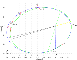
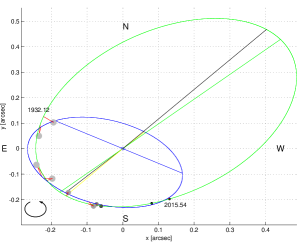
• HIP 85679: The orbit coverage and overall quality of the current fit and data seems to merit to promote it from Grade 5 to Grade 3 in the USNO orbit catalogue. This object was recently reported by Miles & Mason in the IAU Double Stars circular # 191. The listed orbital parameters are $P=220.41$, $T_{0}=1987.21$, $e=0.541$, $a=0.293$, $\omega=252.6$, $\Omega=179.5$, $i=156.3$ (no uncertainties are quoted). These values are in good agreement with our own parameters in Table 2, despite the fact that there is a rather large discrepancy between the dynamical and astrometric mass (see Figure 5), which could indicate a dubious orbital solution. The (dimensionless), mean square error value for our solution is 2.5, while the mean square error for their solution is 8.3 (see the left panel of Figure 9, where we compare both orbits), and their mass sum leads to 4.0$M_{\odot}$ which is slightly smaller than ours at 4.4$M_{\odot}$, and in the right direction (albeit still too large) to agree with an F0V primary. We also note the good agreement between the dynamical and trigonometric parallax for this object on Figure 4 (within $1\sigma$ of the parallax error), so its large astrometric mass sum does not seem to be a consequence of an erroneous parallax. However, the astrometric mass depends very strongly on the assumed parallax, even small changes on the parallax have a big impact on the derived mass, e.g., if we adopt the dynamical parallax instead of the published parallax, the astrometric mass becomes 3.0$M_{\odot}$. Finally, we note the the large difference between $V_{Hip}$ (and $V_{Sim}$) vs. $V_{Sys}$, see Table 1 and Figure 2.

• HIP 85740: Long and undetermined period, very small orbit coverage. Mass sum is too large. However, trigonometric parallax is small and has large error, so mass sum could be reduced importantly by considering a parallax larger by 2$\sigma$ of its error in Table 3. Indeed, increasing the parallax by 2$\sigma$ leads a value of 4.88 mas in consistency with the dynamical parallax, and with a very reasonable astrometric mass of 3.5$M_{\odot}$. Consistency with the dynamical parallax should however be viewed in this case with caution due to the discrepancy noted in Section 2 between $V_{Sys}$ and $V_{Hip}$, $V_{Sim}$ (see also Figure 2). Also, WDS reports an equal magnitude system ($V=8.7$), whereas our own Speckle measurements indicate a $\Delta I=0.5$ (see Table 1), which casts some doubts on the the reported values by WDS, and about the true location of this object on the H-R diagram (see Figure 8). Overall, this is a tentative orbit which could be improved by new observations in a couple of decades.

• HIP 87567: Less than half the orbit is covered, so the period is rather uncertain, but the current orbit seems reasonable as well as the derived mass sum.

• TYC 1566-1708-1: Triple system for which we would need the inner orbit to further improve on the solution. Given its northern declination it is a challenging target for SOAR. Poor orbit coverage (less than half an orbit), leading to a large uncertainty in $P$. No trigonometric parallax available for this target, the eventual addition of a Gaia parallax will be of significant help to study this system further.

• HIP 89076: This object was recently reported by Miles & Mason in the IAU Double Stars circular # 191. The listed orbital parameters are $P=123.84$, $T_{0}=2039.29$, $e=0.450$, $a=0.257$, $\omega=81.9$, $\Omega=240.0$, $i=51.4$ (no uncertainties are quoted). These values are not in agreement with our orbital parameters in Table 2. In Figure 9 (right panel) we compare the two solutions, where we can clearly see that both orbits are reasonable fits to the data points, and that only future observation will allow us to determine a more firm sets of parameters. We also note that the formal mean square error of both solutions are quite different: Ours has 0.098, while theirs (using our weights) has a mean square error of 0.81. Most likely the difference between these two solutions is due to the incomplete orbit coverage and/or due to a choice of different weights per observation, specially on the older data. Their mass sum leads to 1.15$M_{\odot}$, which seems reasonable for a G3V primary. On the other hand, our astrometric mass sum is too small for the spectral type (0.46$M_{\odot}$, see Table 3), but the large discrepancy between the trigonometric and dynamical parallaxes (see Figure 4), added to the rather large parallax uncertainty (of 1.43 mas), implies that we could, e.g., accommodate with our solution, a much larger mass sum (up to 3$M_{\odot}$), for a parallax exactly 3$\sigma$ below the published value, note also that this parallax would be consistent with the computed dynamical parallax. But, even with a parallax smaller than the published value by $1.3\sigma$ the mass sum quartiles for our orbit increase to $(0.85,1.01,1.32)M_{\odot}$. It is interesting to note that we had to apply several quadrant flips to the earlier data, and it is reassuring to see that these are the same flips adopted independently by Miles & Mason, judging from the fit of their orbit to (our) data points.

• HIP 89766: First orbit. Unlike well constrained orbits that have localized solutions, this object exhibits entangled posterior distributions (e.g., in $e$ vs. $T$). Our solution should be considered a surrogate orbit, but otherwise quite uncertain (see also the large quartile mass range in Table 3).

• HIP 91159): Partial coverage of the orbit, rather uncertain period. Due to large period, and despite newer observations, should probably remain in Grade 4, as in the current WDS catalogue. Its orbit is shown in Figure 3.

• HIP 92726: Small coverage of the orbit, long period, but relatively small range in mass quartiles from our MCMC simulation, and the agreement between the ML and quartile solutions warrants promotion to orbit of Grade 4.

• HIP 92909: Orbit seems well defined.

• HIP 93519: The mass sum is too large for its spectral type using the Gaia DR1 parallax ($9.48\pm 0.25$ mas), as can be seen from Figure 5. Interestingly, the Hipparcos parallax ($14.95\pm 3.80$ mas) is much closer to the the dynamical parallax (see Figure 4). For the Hipparcos parallax the mass sum would be 1.9 $M_{\odot}$. However, note that $V_{Sys}$ is suspicious (see Figure 2) and that the system´s color is uncertain (see Table 1), which renders doubts about the dynamical parallax too, and about its true location in the H-R diagram. Its orbit is shown in Figure 3.

• HIP 96317: Poor orbital coverage, long and rather indeterminate period. The highly deviant (speckle) point at 2006.5723 from Hartkopf & Mason (2009), acquired with the Mount Wilson 2.5 m Hooker telescope, can not be explained (even with quadrant flips). Indeed, several quadrant flips were required (note the small $\Delta m$), but those were relatively easy to identify by looking at the $PA$ in reverse chronological order starting from the more recent data. For a trigonometric parallax smaller than $2\sigma$ the quoted uncertainty, the dynamical and astrometric mass sums would however agree at 3.5$M_{\odot}$.

• HIP 99114: First orbit. Based on our solution, in particular, the bounded quartile range for the mass sum and the agreement between dynamical and trigonometric parallaxes in Table 3, it is likely that $3\times\log a-2\times\log P$ should not be grossly erroneous, and so it qualifies as a Grade 4 orbit in the WDS grading system.

• HIP 102945: Well defined orbit. Primary seems to have evolved off MS. Its orbit is shown in Figure 3.

• HIP 103620: First orbit, highly inclined, but well defined. Its orbit is shown in Figure 3.

• HIP 107806: First orbit. Small magnitude difference of the pair ($\Delta V=0.51$, $\Delta I=0.2$, with several plausible quadrant flips. Quadrant ($PA=122.0$ deg) firmly determined from lucky imaging in last data point at 2015.4971 helps resolve earlier ambiguities. Large (more than $6\sigma$) discrepancy between the trigonometric and dynamical parallax. A parallax smaller by $3\sigma$ gives an astrometric mass sum of $1.1M_{\odot}$.

• HIP 109908: The primary seems to have evolved off the MS, as suggested in Figure 8. The spectral type for the primary is indeed listed as G8III in SIMBAD (hence the dynamical mass - which assumes class V - would be erroneous, see Figure 4), while the computed color and absolute magnitude for the secondary imply a spectral type of about A6. Still the astrometric mass seem too large despite of an orbit that appears relatively well determined.

• HIP 114962: Residuals show a hint of a possible sub-system, but current data does not warrant a solution for that. This is the only object for which we have a published $I_{Sim}=7.37$. The primary and secondary $I$-band magnitudes computed in the way described at the beginning of this section, leads to $I_{P}=8.03$ and $I_{S}=8.63$, or an equivalent $I_{Sys}=7.54$, which compares well with the literature value indicated above, considering our estimated uncertainty of 0.18 mag for $\Delta I$, as explained in Section 2 (and it even suggests that perhaps our $I$-band (and colors) errors are somewhat overestimated).

Figure 9: Orbits for two of our objects, compared to recently published results. Left panel is for HIP 85679, right panel is for HIP 89076. Blue orbit is from our MCMC solution, green orbit is from IAU Double Stars circular # 191. The adoption of different weights to each datum might be responsible for the differences in the fits.

We finally note that tables with the adopted weights for each data entry (see Section 2), the adopted quadrant flips (see Section 3), and the $O-C$ values for all our solutions can be requested from the principal author.

5 Conclusions

In 2014 we started a systematic campaign with the speckle camera HRCAM on the 4m SOAR telescope at CTIO to observe Hipparcos binaries and spectroscopic binaries from the Geneva-Copenhagen spectroscopic survey in the Southern sky with the purpose of computing their orbits, and determining their masses. This work will complement and significantly extend the WIYN Northern sky speckle program lead by Horch and collaborators, allowing us to compile an all-sky, volume-limited speckle survey of these two primary samples, allowing us to investigate effects such as metallicity and age on the MLR.

In this paper we have presented orbital elements and mass sums for eighteen visual binary stars of spectral types B to K (five of which are new orbits) with periods ranging from 20 to more than 500 yr, and individual component masses with a formal uncertainty of $\sim 0.1M_{\odot}$ for two double-line spectroscopic binaries with no previous orbits using combined astrometric plus radial velocity data. Using published optical photometry and trigonometric parallaxes, plus our own measurements, we put these objects on an H-R diagram, and briefly discuss their evolutionary status. Cases where one (or both) components have evolved off of the main sequence are particularly interesting, since for them an age determination is also possible (a hint of this can be seen for HIP 109908, see Figure 8). However, to do this properly, it is critical to have not only reliable parallaxes (which Gaia will provide), but also good multi-color photometry for the individual components - which is challenging, specially for the tighter systems.

To compute the orbital elements we have developed a MCMC algorithm that produces maximum likelihood estimates as well as posterior PDFs of the parameters given the measurements that allow us to evaluate the uncertainty of our derived orbital elements in a robust way. In the case of the spectroscopic binaries, and inspired by the work of Wright & Howard (2009) in the context of exoplanets (where the primary is considered basically at rest), we present a mathematical formalism in which we generalize their approach to the case of binary systems (where both components have a sizeable motion) to achieve a significant dimensionality reduction from seven to three dimensions in the case of visual binaries, and from ten to seven dimensions (including orbital parallax) in the case of spectroscopic binaries with astrometric data. Our self-consistent solution for orbital parallax will be particularly useful when comparing to Gaia’s high precision trigonometric parallaxes. Furthermore, this dimensionality reduction implies that we only need to explore a reduced subset of the parameter space, thus reducing significantly the computational cost. The remaining parameters are determined by a simple least-squares linear fit to the data and the significant parameters. Although in this case we have chosen to use an MCMC approach for parameter exploration, our formalism for dimensionality reduction is completely general, and can be used with other parameter exploration-based methods.

In a future paper we will apply the MCMC approach outlined here to interesting cases where partial data (see e.g., Claveria et al. (2016)), non-resolutions, or other sources of information (e.g., spectral type) are available, information which can be easily incorporated as constraining priors into our Bayesian code, and which become crucial specially in cases of objects with very limited observational coverage which prevents us from estimating an orbit yet with adequate precision, but for which one might desire to have more reliable tentative ephemerides for observational planning.

6 Acknowledgments

We acknowledge Dr. Andrei Tokovinin from CTIO and Dr. Elliot Horch from Southern Connecticut State University for all their support throughout this entire research, including the stages of telescope time application, data acquisition, calibration and analysis, as well as their suggestions for improvement to the original manuscript. We also acknowledge Dr. Jose Angel Docobo (Universidad de Santiago de Compostela, Spain) and Venu Kalari (FONDECYT/CONICYT Postdoctoral Fellow Universidad de Chile) for their reading and suggestions to the original manuscript, and the referee Dr. Dimitri Pourbaix (Institute of Astronomy and Astrophysics, Université Libre de Bruxelles, Brussels) for many suggestions and corrections that have significantly improved the readability of the paper. This research has made use of the Washington Double Star Catalog maintained at the U.S. Naval Observatory and of the SIMBAD database, operated at CDS, Strasbourg, France. This work has made use of data from the European Space Agency (ESA) mission Gaia (https://www.cosmos.esa.int/gaia), processed by the Gaia Data Processing and Analysis Consortium (DPAC, https://www.cosmos.esa.int/web/gaia/dpac/consortium). Funding for the DPAC has been provided by national institutions, in particular the institutions participating in the Gaia Multilateral Agreement. Based on Chilean telescope time under programs CN2014B-27, CN2015B-6, and CN2016A-4.

RAM acknowledges support from the Chilean Centro de Excelencia en Astrofísica y Tecnologías Afines (CATA) BASAL PFB/06, from the Project IC120009 Millennium Institute of Astrophysics (MAS) of the Iniciativa Científica Milenio del Ministerio de Economía, Fomento y Turismo de Chile, and from CONICYT/FONDECYT Grant Nr. 1151213. RMC has been supported by a MSc scholarship from CONICYT, Chile (CONICYT-PCHA/Magister Nacional/2016-22162232). MEO acknowledges support from CONICYT/FONDECYT Grant Nr. 1170044. JSF acknowledges support from CONICYT/FONDECYT Grant Nr. 1170854. MEO and JSF also acknowledge support from the Advanced Center for Electrical and Electronic Engineering, Basal Project FB0008, and from CONICYT PIA ACT1405.

Appendix A Keplerian model equations

Calculating the position $(\rho,\theta)$ of the relative orbit (or the equivalent Cartesian coordinates) at a certain instant of time $\tau$ involves a sequence of steps, as described as follows:

• Solving Kepler’s Equation in order to obtain the eccentric anomaly $E$.

  $$2\pi(\tau-T)/P=E-e\sin E.$$ (A1)

• Computing the auxiliary values $x$, $y$, referred to as normalized coordinates hereinafter.

  $$x(E)=\cos E-e,$$ (A2)

  $$y(E)=\sqrt{1-e^{2}}\sin E.$$

• Determining the Thiele-Innes constants.

  $$A= ~{}a(\cos\omega~{}\cos\Omega-\sin\omega~{}\sin\Omega~{}\cos i),$$ (A3)

  $$B= ~{}a(\cos\omega~{}\sin\Omega+\sin\omega~{}\cos\Omega~{}\cos i),$$

  $$F= ~{}a(-\sin\omega~{}\cos\Omega-\cos\omega~{}\sin\Omega~{}\cos i),$$

  $$G= ~{}a(-\sin\omega~{}\sin\Omega+\cos\omega~{}\cos\Omega~{}\cos i).$$

• Calculating the position in the apparent orbit as:

  $$X=Bx+Gy$$ (A4)

  $$Y=Ax+Fy.$$

In the case of spectroscopic binaries, one aims to adjust the Keplerian model to radial velocity data as well. This is accomplished by a somewhat different sequence of steps:

• Use the $E$ value (Equation A1) to calculate the true anomaly $\nu$ at certain epoch of observation $\tau$:

  $$\tan\frac{\nu}{2}=\sqrt{\frac{1+e}{1-e}}\tan\frac{E}{2}.$$ (A5)

• Calculate the model’s radial velocity through the following equations:

  $$V_{primary}=V_{CoM}+\frac{2\pi a_{P}\sin i}{P\sqrt{1-e^{2}}}\left[\cos(\omega+\nu)+e\cos\omega\right]=V_{CoM}+K_{P}\left[\cos(\omega+\nu)+e\cos\omega\right],$$ (A6)

  $$V_{secondary}=V_{CoM}-\frac{2\pi a_{S}\sin i}{P\sqrt{1-e^{2}}}\left[\cos(\omega+\nu)+e\cos\omega\right]=V_{CoM}-K_{S}\left[\cos(\omega+\nu)+e\cos\omega\right],$$ (A7)

  where $a_{P}$ is calculated as $a^{\prime\prime}/\varpi\cdot q/(1+q)$ and $a_{S}=a^{\prime\prime}/\varpi\cdot 1/(1+q)$, where $q\leq 1$ is the mass ratio $m_{S}/m_{P}$.

A.1 On the dimensionality of $\vec{\vartheta}$

Since the set of objects studied in this work makes up a relatively long list, it seems reasonable to devote some effort to reduce the computational costs involved in the analysis. In exploration-based methods such as the MCMC technique, the computer time required to obtain good results (in terms of convergence, precision and accuracy of the estimates) grows as the dimension of the feature space increases. For that reason, and at the expense of not exploring the whole seven-dimensional feature space of orbital parameters (ten-dimensional space in the case of spectroscopic binaries), we propose a dimensionality reduction based on the separation of the parameter vector into two lower dimension vectors: one containing components whose least-squares solution cannot be determined analytically ($\vec{\vartheta}_{1}$); and the other containing the components whose linear dependency makes it possible to calculate their least-squares solution with simple matrix algebra ($\vec{\vartheta}_{2}$).

In the case of binaries with astrometric measurements only, one exploits the linear dependency of the well-known Thiele-Innes constants ($A$, $B$, $G$, $F$) with respect to the normalized coordinates $x$, $y$ (which in turn depend on $P$, $T$, $e$ and the collection of epochs of observation, $\{\tau_{i}\}_{i=1,\dots,N}$). The procedure to obtain the least-squares solution of Thiele-Innes is detailed in Appendix B.1. Thus, instead of exploring the whole 7D space, the search is focused on $\vec{\vartheta}_{1}=[P,T,e]$, with $\vec{\vartheta}_{2}=[A,B,F,G]$ determined individually from each combination of the free parameters in $\vartheta_{1}$. The Campbell elements $a$, $\omega$, $\Omega$, $i$ can be recovered by using equations A8 (the detailed procedure is shown in Appendix B.2). We followed the convention of choosing solutions with $\Omega\in(0^{\circ},180^{\circ})$ in absence of information about the real orientation of the orbit.

$$tan(\omega+\Omega)=\frac{B-F}{A+G},$$ (A8)

$$tan(\omega-\Omega)=\frac{-B-F}{A-G},$$

$$a^{2}(1+\cos^{2}i)=A^{2}+B^{2}+F^{2}+G^{2},$$

$$a^{2}\cos^{2}i=AG-BF.$$

Some definitions must be introduced before describing the approach adopted by us for binaries with spectroscopic data. In addition to the four parameters A, B, F, G, the Thiele-Innes representation uses parameters $C$ to $H$ to compute the coordinates in the Z-axis (along the line-of-sight):

$$Z=Cx+Hy.$$ (A9)

These quantities are defined as follows:

$$C=a~{}\sin\omega~{}\sin i,$$ (A10)

$$H=a~{}\cos\omega~{}\sin i.$$

In Wright & Howard (2009), the authors take advantage of this representation to propose an efficient method to fit multi-Keplerian models to purely spectroscopic, purely astrometric, and combined data sets. The core of their approach is the reformulation of equations A6 and A7 in a manner such that $V_{P}$ and $V_{S}$ are linear in the parameters, allowing for analytic calculation of least-square solutions. Making use of some trigonometric identities, the radial velocity equation can be expressed as:

$$V(\tau)=h\cos\nu(\tau)+c\sin\nu(\tau)+\gamma,$$ (A11)

where $h=K\cos\omega$, $c=-K\sin\omega$, $\gamma=V_{CoM}+K\cdot e\cdot\cos\omega$. Thus, $h=H/\varpi\cdot 2\pi/(P\sqrt{1-e^{2}})$, $c=-C/\varpi\cdot 2\pi/(P\sqrt{1-e^{2}})$.

Since that paper was targeted at exoplanet research, each body involved is modeled with an independent Keplerian orbit, omitting the influence that each component of the system exerts on the other. However, that influence is not negligible when analyzing objects with masses of similar order of magnitude, and therefore that approach is not directly applicable to binary stars. Concretely, when analyzing binary stars, the conditions shown below must be met, making the orbital parameters of the primary and those of the secondary interdependent.

$$a~{}= a_{P}+a_{S},$$ (A12)

$$\frac{a_{P}}{a_{S}}= \displaystyle\frac{m_{S}}{m_{P}}=q,$$

The equalities above impose constraints on the parameters being estimated: if we reformulate equations A6, A7 according to the parameterization presented in Equation A11, then $h_{P}=H_{P}/\varpi\cdot 2\pi/(P\sqrt{1-e^{2}})$, $c_{P}=-C_{P}/\varpi\cdot 2\pi/(P\sqrt{1-e^{2}})$, being $H_{P}=a_{P}\cos\omega\sin i=\frac{q}{1+q}H$, $C_{P}=a_{P}\sin\omega\sin i=\frac{q}{1+q}C$ (analogous equations for $V_{S}$: specifically, $H_{S}=\frac{1}{1+q}H$, $C_{S}=\frac{1}{1+q}C$). The strict relations that $(H_{P},C_{P})$ and $(H_{S},C_{S})$ must comply (namely, $H=H_{P}+H_{S}$, $C=C_{P}+C_{S}$, $H_{P}/H_{S}=C_{P}/C_{S}=q$) do not stem naturally when calculating these quantities as free parameters. Therefore, those conditions must be enforced as an additional mathematical restriction in the model.

Although one could address the interdependence problem raised in the previous paragraph using Lagrange multipliers, there is no guarantee that the resulting set of non-linear equations will be analytically tractable (it may even have no unique solution). However, one can manipulate the formulae in a manner such that both orbital and radial velocity values of the Keplerian model are expressed as a linear combination of parameters, and meet the restrictions mentioned in the paragraph above at the same time:

• In an approach similar to that used in Wright & Howard (2009), the first step is to use a combination of H and C – which are simpler expressions – to reconstruct parameters A, B, F and G (this requires the aim of trigonometric functions of $\Omega$ and $i$):

  (A13)

• Grouping the terms multiplying $C$ and $H$ yields:

  (A14)

  Thus, the coordinates X, Y can be written as a linear combination of terms $S_{X}$, $T_{X}$, $S_{Y}$, $T_{Y}$ (which can be easily computed from $x$, $y$, $\Omega$ and $i$), being $H$ and $C$ their accompanying constants.

• Finally, by using $\lambda_{P}=\frac{q}{1+q}\cdot\frac{2\pi}{\varpi P\sqrt{1-e^{2}}}$, $\lambda_{S}=\frac{1}{1+q}\cdot\frac{2\pi}{\varpi P\sqrt{1-e^{2}}}$ to transform $H$, $C$ into $h_{P}$, $h_{S}$, $c_{P}$, $c_{S}$, one can express both the astrometric coordinates (Equation A4) and radial velocity values (equations A6, A7) in terms of a vector of parameters $\vec{\vartheta}_{2}=[H,C,V_{CoM}]$:

  $$\vec{\vartheta}_{2}\cdot\mathbf{F}=[\vec{X}^{model},\vec{Y}^{model},\vec{V_{P}}^{model},\vec{V_{S}}^{model}],$$ (A15)

  where $\mathbf{F}$ is:

  (A16)

  This allows for the calculation of the least-squares solution for $\vec{\vartheta}_{2}$ as (see, e.g., Kay (1993)):

  $$\vec{\vartheta}_{2}=\vec{x}~{}\mathbf{W}\mathbf{F}^{T}(\mathbf{F}\mathbf{W}\mathbf{F}^{T})^{-1},$$ (A17)

  where $\vec{x}=[\vec{X}^{obs},\vec{Y}^{obs},\vec{V_{P}}^{obs},\vec{V_{S}}^{obs}]$ is the data vector and $\mathbf{W}$ is a diagonal matrix with the weight of each observation. From the resulting $\hat{H}$ and $\hat{C}$ values (the values with a hat represent a particular estimate of that quantity, based on the current data), the parameters $a$ and $\omega$ can be recovered as follows:

  $$\hat{a} =\displaystyle\sqrt{\frac{\hat{C}^{2}+\hat{H}^{2}}{\sin^{2}i}},$$ (A18)

  $$\hat{\omega} =\displaystyle\tan^{-1}\left(\frac{\hat{C}}{\hat{H}}\right),$$ (A19)

  The third component of $\vec{\vartheta}_{2}$ ($V_{CoM}$) has direct physical meaning and does not need to be transformed. Under this scheme, only seven parameters ($P$, $T$, $e$, $\Omega$, $i$, $q$, $\varpi$) must be explored and estimated, whereas $a$, $\omega$ and $V_{CoM}$ are calculated analytically. Although in this work we use the MCMC technique, the representation developed here – and the dimensionality reduction that it involves – can be applied to other sorts of methods as well, even if they are not strictly exploration-based, such as the Levenberg-Marquardt algorithm.

Appendix B On Thiele-Innes and Campbell elements

B.1 Least-squares estimate

The starting point is the sum of individual errors:

$$\sum_{k=1}^{N_{x}}\frac{1}{\sigma_{x}^{2}(k)}[X(k)-X^{model}(k)]^{2}+\sum_{k=1}^{N_{y}}\frac{1}{\sigma_{y}^{2}(k)}[Y(k)-Y^{model}(k)]^{2}$$ (B1)

Equation A4 enables us to replace $X_{model}$, $Y_{model}$ with their analytic expression for any epoch (indexed by $k$):

$$X_{obs}(k)-X_{model}(k) =X_{obs}(k)-[B\cdot x(k)+G\cdot y(k)]$$ (B2)

$$Y_{obs}(k)-Y_{model}(k) =Y_{obs}(k)-[A\cdot x(k)+F\cdot y(k)].$$

Given the linear dependency of $X_{model}$, $Y_{model}$ with respect to the normalized coordinates $x$, $y$, it is possible to calculate a least-squares estimate for the unknown variables $B$, $G$, $A$, $F$ in a non-iterative way. Moreover, the first term of Equation B1 depends only on the pair $(B,G)$, whereas the second term depends on the pair $(A,F)$. Therefore, the estimate for $(B,G)$ is obtained by minimizing the first term and the estimate for $(A,F)$ by minimizing the second one, independently. The problem is thus reduced to a pair of uncoupled linear equations. By calculating the derivatives of the expression of the error with respect to each of the Thiele-Innes constants and making the results equal to zero, one can obtain the following formulae (for the sake of briefness, a set of auxiliary terms is introduced first):

$$\alpha=\sum_{i}~{}w_{i}~{}x(i)^{2}~{}~{}~{}~{}~{}~{} \beta=\sum_{i}~{}w_{i}~{}y(i)^{2} \gamma=\sum_{i}~{}w_{i}~{}x(i)~{}y(i)$$

$$r_{11}=\sum_{i}~{}w_{i}~{}X_{obs}(i)~{}x(i) r_{12}=\sum_{i}~{}w_{i}~{}X_{obs}(i)~{}y(i)$$ (B3)

$$r_{21}=\sum_{i}~{}w_{i}~{}Y_{obs}(i)~{}x(i) r_{22}=\sum_{i}~{}w_{i}~{}Y_{obs}(i)~{}y(i)$$

Then, the least-squares estimate for the Thiele-Innes set of parameters is calculated as follows:

$$\hat{B}=\frac{\beta\cdot r_{11}-\gamma\cdot r_{12}}{\Delta},~{}~{}~{}~{}~{}~{} \hat{G}=\frac{\alpha\cdot r_{12}-\gamma\cdot r_{11}}{\Delta},$$ (B4)

$$\hat{A}=\frac{\beta\cdot r_{21}-\gamma\cdot r_{22}}{\Delta},~{}~{}~{}~{}~{}~{} \hat{F}=\frac{\alpha\cdot r_{22}-\gamma\cdot r_{21}}{\Delta},$$

where $\Delta=\alpha\cdot\beta-\gamma^{2}$.

B.2 Conversion from Thiele-Innes to Campbell constants

Once the estimates ($\hat{B}$, $\hat{G}$, $\hat{A}$, $\hat{F}$) for the Thiele-Innes constants are obtained, it is necessary to recover the equivalent representation in terms of the Campbell elements ($a,\omega,\Omega,i$). For $\omega$ and $\Omega$, one must solve the following set of equations:

$$\omega+\Omega =\arctan\left(\frac{B-F}{A+G}\right),$$ (B5)

$$\omega-\Omega =\arctan\left(\frac{-B-F}{A-G}\right),$$

choosing the solution that satisfies that $\sin(\omega+\Omega)$ has the same sign as $B-F$ and that $\sin(\omega-\Omega)$ has the same sign as $-B-F$. If that procedure outputs a value of $\Omega$ that does not satisfy the convention that $\Omega\in(0,\pi)$, it must be corrected in the following way: if $\Omega<0$, values of $\omega$ and $\Omega$ are modified as $\omega=\pi+\omega$, $\Omega=\pi+\Omega$; whereas if $\Omega>\pi$, values of $\omega$ and $\Omega$ are modified as $\omega=\omega-\pi$, $\Omega=\Omega-\pi$.

For semi-major axis $a$ and inclination $i$, the following auxiliary variables must be calculated first:

$$k =\frac{A^{2}+B^{2}+F^{2}+G^{2}}{2},$$

$$m =A\cdot G-B\cdot F,$$ (B6)

$$j =\sqrt{k^{2}-m^{2}}.$$

Then, $a$ and $i$ are determined with the following formulae:

$$a =\sqrt{j+k}$$ (B7)

$$i =\arccos\left(\frac{m}{a^{2}}\right)$$

Appendix C Algorithms for parameter estimation

Figure 10 outlines DE-MC procedure used for visual binaries, whereas the pseudo-code in Figure 11 describes the Gibbs sampler used for spectroscopic binaries.

Figure 10: Differential Evolution Markov Chain: This algorithm relies on running several chains in parallel, and letting them learn from each other. To do so, on each iteration $i$ and for each chain $j$, two different chains $j_{1}\neq j$ and $j_{2}\neq j$ are chosen at random, and the difference between their current states, $x^{(i-1,j_{1})}-x^{(i-1,j_{2})}$, is used to propose new samples $x^{\prime}$, which are accepted (or rejected) according to the Metropolis-Hastings criterion. Since we perform a dimensionality reduction in the parameter vector of visual binaries, $x\equiv\vec{\vartheta}_{1}=[P,T^{\prime},e]$ in our implementation. The pseudo-code in this figure details the procedure.

If the parameter vector is $x=[x_{1},\dots,x_{d}]$, then Gibbs sampler operates as follows:

Figure 11: To sample the posterior distribution of spectroscopic binaries, we have used a Metropolis-Hastings-within-Gibbs approach. A proposal distribution $q_{j}^{\prime}$ is defined: let $x^{(i)}_{-j}$ be $[x_{1}^{(i)},\dots,x_{j-1}^{(i)},x_{j+1}^{(i)},\dots,x_{d}^{(i)}]$ (all components other than $j$), then $q_{j}^{\prime}(x|x^{(i)})$ is a distribution that induces leaps only on the $j$-th component (i.e., $x_{-j}$ remains equal to $x_{-j}^{(i)}$, while $x_{j}$ is the result of a random variation on $x_{j}^{(i)}$). Thus, the Metropolis-Hastings-within-Gibbs algorithm operates as shown in this pseudo-code, where $x\equiv\vec{\vartheta}_{1}=[P,T^{\prime},e,\omega,i,q,\varpi]$ as our vector of interest.

References

- Andrieu et al. (2003) Andrieu, C., De Freitas, N., Doucet, A., and Jordan, M. I. 2003, Machine learning, 50, 5
- Altmann & Bouquillon (2016) Altmann, M., & Bouquillon, S. 2016, private communication
- Braak (2006) Braak, C. J. T. 2006, Statistics and Computing, 16, 239
- Burgasser et al. (2015) Burgasser, A. J., Melis, C., Todd, J., et al. 2015, AJ, 150, 180
- Claveria et al. (2016) Claveria, R. M., Acuna, D. E., Mendez, R. A., Silva, J. F., and Orchard, M. E. 2016, Annual Conference of the Prognostics and Health Management Society, 7, 1
- Davidson et al. (2009) Davidson, J. W., Jr., Baptista, B. J., Horch, E. P., Franz, O., & van Altena, W. F. 2009, AJ, 138, 1354
- Dieterich et al. (2012) Dieterich, S. B., Henry, T. J., Golimowski, D. A., Krist, J. E., & Tanner, A. M. 2012, AJ, 144, 64
- Docobo & Andrade (2013) Docobo, J. A., & Andrade, M. 2013, MNRAS, 428, 321
- Duquennoy & Mayor (1991) Duquennoy, A., & Mayor, M. 1991, A&A, 248, 485
- Eddington (1924) Eddington, A. S. 1924, MNRAS, 84, 308
- Eggen (1967) Eggen, O. J. 1967, ARA&A, 5, 105
- Ford (2005) Ford, E. B. 2005, AJ, 129, 1706
- Fuhrmann et al. (2017) Fuhrmann, K., Chini, R., Kaderhandt, L., & Chen, Z. 2017, ApJ, 836, 139
- Gaia Collaboration et al. (2016) Gaia Collaboration, Prusti, T., de Bruijne, J. H. J., et al. 2016, A&A, 595, A1
- Gao et al. (2014) Gao, S., Liu, C., Zhang, X., et al. 2014, ApJ, 788, L37
- Gelman et al. (2013) Gelman, A., Carlin, J. B., Stern, H. S., Dunson, D. B., Vehtari, A., and Rubin, D. B. 2013, Bayesian Data Analysis , CRC Press
- Geman & Geman (1984) Gemans, S. & Geman, D. 1984, IEEE Transactions on pattern analysis and machine intelligence, 6, 721
- Ghosh et al. (2004) Ghosh, H., DePoy, D. L., Gal-Yam, A., et al. 2004, ApJ, 615, 450
- Gould et al. (2004) Gould, A., Bennett, D. P., & Alves, D. R. 2004, ApJ, 614, 404
- Gould (2014) Gould, A. 2014, Journal of Korean Astronomical Society, 47, 215
- Greenwood (1977) Greenwood, D. P. 1977, Journal of the Optical Society of America (1917-1983), 67, 390
- Gregory (2005) Gregory, P. C. 2005, ApJ, 631, 1198
- Griffin (1999) Griffin, R. F. 1999, The Observatory, 119, 81
- Hartkopf et al. (1989) Hartkopf, W. I., McAlister, H. A., & Franz, O. G. 1989, AJ, 98, 1014
- Hartkopf et al. (2001) Hartkopf, W. I., Mason, B. D., & Worley, C. E. 2001, AJ 122, 3472
- Hartkopf & Mason (2009) Hartkopf, W. I., & Mason, B. D. 2009, AJ, 138, 813
- Henry & McCarthy (1993) Henry, T. J., & McCarthy, D. W., Jr. 1993, AJ, 106, 773
- Hestroffer (2012) Hestroffer, D. 2012, Orbital Couples: Pas de Deux in the Solar System and the Milky Way, 113
- Horch & van Altena (2011) Horch, E. P., & van Altena, W. F. 2011, American Institute of Physics Conference Series, 1346, 21
- Horch et al. (2011) Horch, E. P., Gomez, S. C., Sherry, W. H., et al. 2011, AJ, 141, 45
- Horch et al. (2015) Horch, E. P., van Altena, W. F., Demarque, P., et al. 2015, AJ, 149, 151
- Horch et al. (2017) Horch, E. P., Casetti-Dinescu, D. I., Camarata, M. A., et al. 2017, arXiv:1703.06253
- Iben (2013) Iben, I. 2013, Stellar Evolution Physics, Vols. 1 and 2, Cambridge University Press
- Kahler (1972) Kahler, H. 1972, A&A, 20, 105
- Kay (1993) Kay, S. M. 1993, Fundamentals of statistical signal processing, volume I: estimation theory, Prentice Hall
- Kippenhahn et al. (2012) Kippenhahn, R., Weigert, A., & Weiss, A. 2012, Stellar Structure and Evolution: , Astronomy and Astrophysics Library. ISBN 978-3-642-30255-8. Springer-Verlag
- Lindegren et al. (1997) Lindegren, L., Mignard, F., Söderhjelm, S., et al. 1997, A&A, 323, L53
- Lucy (2014) Lucy, L. B. 2014, A&A, 563, A126
- Marion et al. (2014) Marion, L., Absil, O., Ertel, S., et al. 2014, A&A, 570, A127
- Mason (2015) Mason, B. D. 2015, IAU General Assembly, 23, 2300709
- Massey et al. (2001) Massey, P., Meyer, M., & Murdin, P. 2001, Encyclopedia of Astronomy and Astrophysics, Edited by Paul Murdin, article 1882. Bristol: Institute of Physics Publishing.
- MacKnight & Horch (2004) MacKnight, M., & Horch, E. P. 2004, Bulletin of the American Astronomical Society, 36, 07.19
- Marigo et al. (2017) Marigo, P., Girardi, L., Bressan, A., et al. 2017, ApJ, 835, 77
- Mede & Brandt (2014) Mede, K., & Brandt, T. D. 2014, Exploring the Formation and Evolution of Planetary Systems, 299, 52
- Mendez & van Altena (1998) Mendez, R. A., & van Altena, W. F. 1998, A&A, 330, 910
- Nordström et al. (2004) Nordström, B., Mayor, M., Andersen, J., et al. 2004, A&A, 418, 989
- Otor et al. (2016) Otor, O. J., Montet, B. T., Johnson, J. A., et al. 2016, AJ, 152, 165
- Platais et al. (2003) Platais, I., Pourbaix, D., Jorissen, A., et al. 2003, A&A, 397, 997
- Pourbaix & Lampens (1999) Pourbaix, D., & Lampens, P. 1999, Harmonizing Cosmic Distance Scales in a Post-HIPPARCOS Era, 167, 300
- Pourbaix (2000) Pourbaix, D. 2000, A&AS, 145, 215
- Pourbaix et al. (2004) Pourbaix, D., Tokovinin, A. A., Batten, A. H., et al. 2004, A&A, 424, 727
- Raghavan et al. (2010) Raghavan, D., McAlister, H. A., Henry, T. J., et al. 2010, ApJS, 190, 1
- Sahlmann et al. (2013) Sahlmann, J., Lazorenko, P. F., Ségransan, D., et al. 2013, A&A, 556, A133
- Söderhjelm (1999) Söderhjelm, S. 1999, A&A, 341, 121
- Storn & Price (1997) Storn, R., & Price, K. 1997, Journal of global optimization, 11, 341
- van Altena & Lee (1988) van Altena, W. F., & Lee, J. T. 1988, In ESA Seismology of the Sun and Sun-Like Stars, 286, 649
- Tokovinin (1992) Tokovinin, A. 1992, IAU Colloq. 135: Complementary Approaches to Double and Multiple Star Research, 32, 573
- Tokovinin et al. (2010) Tokovinin, A., Mason, B. D., & Hartkopf, W. I. 2010, AJ, 139, 743
- Tokovinin (2012) Tokovinin, A. 2012, AJ, 144, 56
- Tokovinin et al. (2014) Tokovinin, A., Mason, B. D., & Hartkopf, W. I. 2014, AJ, 147, 123
- Tokovinin (2014) Tokovinin, A. 2014, AJ, 147, 86
- Tokovinin et al. (2015) Tokovinin, A., Mason, B. D., Hartkopf, W. I., Mendez, R. A., & Horch, E. P. 2015, AJ, 150, 50
- Tokovinin et al. (2016) Tokovinin, A., Mason, B. D., Hartkopf, W. I., Mendez, R. A., & Horch, E. P. 2016, AJ, 151, 153
- Tuomi & Kotiranta (2009) Tuomi, M., & Kotiranta, S. 2009, A&A, 496, L13
- Wright & Howard (2009) Wright, J. T., & Howard, A. W. 2009, ApJS, 182, 205
- Yuan et al. (2015) Yuan, H., Liu, X., Xiang, M., et al. 2015, ApJ, 799, 135