Scalable Estimation of Dirichlet Process Mixture Models on Distributed Data

Abstract

We consider the estimation of Dirichlet Process Mixture Models (DPMMs) in distributed environments, where data are distributed across multiple computing nodes. A key advantage of Bayesian nonparametric models such as DPMMs is that they allow new components to be introduced on the fly as needed. This, however, posts an important challenge to distributed estimation – how to handle new components efficiently and consistently. To tackle this problem, we propose a new estimation method, which allows new components to be created locally in individual computing nodes. Components corresponding to the same cluster will be identified and merged via a probabilistic consolidation scheme. In this way, we can maintain the consistency of estimation with very low communication cost. Experiments on large real-world data sets show that the proposed method can achieve high scalability in distributed and asynchronous environments without compromising the mixing performance.

1 Introduction

Dirichlet Process Mixture Models (DPMMs) Antoniak (1974) is an important family of mixture models, which have received much attention from the statistical learning community since its inception. Compared to classical mixture models for which the number of components has to be specified a priori, DPMMs allow the model size to change as needed. Hence, they are particularly suited to exploratory study, especially in the contexts that involve massive amount of data.

Various methods have been developed for estimating DPMMs from data. From earlier methods based on the Chinese Restaurant Process (CRP) formulation MacEachern and Müller (1998) to recent ones that resort to merge-split steps Jain and Neal (2004) or variational formulations Blei and Jordan (2005), the performance has been substantially improved. Most of these methods adopt a serial procedure, where updating steps have to be executed sequentially, one after another. As we move steadily towards the era of big data, Bayesian nonparametrics, like many other machine learning areas, is faced with a significant challenge, namely, to handle massive data sets that may go beyond the capacity of a single computing node. Tackling such a challenge requires new techniques that can process different parts of the data concurrently. However, most existing methods for DPMM estimation adopt an iterative procedure, and therefore they are not able to scale in a distributed environment.

In recent years, parallel methods Williamson et al. (2013); Chang and Fisher III (2013) have been developed, which attempt to speed up the estimation of DPMMs through parallel processing, by exploiting the conditional independence of the model. Note that these parallel methods are based on the shared memory architecture, where the entire dataset together with the intermediate results are held in a unified memory space, and all working threads can access them without costly communication. However, in large-scale applications, the amount of data can go far beyond the capacity of a single computer. Handling such data requires a distributed architecture, where multiple computers, each called a computing node, are connected via communication channels with limited bandwidth, e.g. Ethernet. Computing nodes do not share memory – information exchange has to be done via communication. The parallel methods mentioned above, when applied to such settings, would incur considerable communication costs. For example, changing associations between samples and processors can result in frequent data transfer.

In this work, we aim to develop a new method for DPMM estimation that can scale well on a distributed computing architecture. Distributed estimation is not a new story – a variety of methods for estimating parametric models from distributed data Newman et al. (2009) have been developed in recent years. However, nonparametric models like DPMMs, present additional challenges due to the possibility of new components being introduced on the fly. Therefore, how to handle new components efficiently and consistently becomes an important issue. On one hand, to attain high concurrency, one has to allow local workers to discover new components independently; on the other hand, components arising from different workers may actually correspond to the same cluster, which need to be identified and merged in order to form a coherent estimation. The trade-off between mixing performance and communication cost is also an important issue.

In tackling this problem, we develop a distributed sampling algorithm, which allow new components to be introduced by local workers, while maintaining the consistency among them through two consolidation schemes, namely progressive consolidation and pooled consolidation. We tested the proposed methods on both synthetic and large real-world datasets. Experimental results show that they can achieve reasonably high scalability while maintaining the convergence speed. It is also worth noting that the proposed method can work under asynchronous settings without performance degradation.

2 Related Work

With the rapid growth of data, parallel and distributed methods have received increasing attention. Earlier efforts along this line focused on the estimation of parametric models. Newman et al Newman et al. (2007, 2009) presented a method for estimating LDA models Blei et al. (2003) on distributed data, where concurrent sampling on local subsets of data are followed by a global update of the topic counts. Smyth et al Smyth et al. (2009) further extend this algorithm to asynchronous settings. All these methods assume a fixed parameter space, and therefore they can not be directly used for estimating Bayesian nonparametric models, of which the size of the parameter space can vary on the fly.

For DPMMs, a variety of estimation methods based on different theoretical foundations have been developed, such as Chinese Restaurant Process MacEachern and Müller (1998), stick-breaking reconstruction Sethuraman (1994), Poisson processes Lin et al. (2010), and slice sampling Walker (2007). The serial nature of these methods make them difficult to be parallelized.

Driven by the trend of concurrent computing, recent years witnessed new efforts devoted to parallel estimation of BNP models. Chang and Fisher Chang and Fisher III (2013) proposed an MCMC algorithm that accomplishes both intra-cluster and inter-cluster parallelism by augmenting the sample space with super-cluster groups. In the same year, Williamson et al Williamson et al. (2013) proposed another parallel sampler for DPMMs, which exploits the conditional independence among components through auxiliary weights. Assuming that all processors share memory, both methods update associations between samples and processors in each iteration. Hence, they are not suitable for distributed estimation where information can only be exchanged across limited communication channels. Also, it has been found Gal and Ghahramani (2014) that some parallel methods such as Williamson et al. (2013) have the issue of unbalanced workload among processors.

Recently, attempts have been made to further extend BNP estimation to distributed environments. Ge et al Ge et al. (2015) developed a distributed estimation method for DPMMs based on the slice sampler presented in Walker (2007). This method adopts a map-reduce paradigm, where the map step is to sample component labels, while the reduce step is to accumulate component weights, update parameters, or create new components. This method has a limitation: new components are sampled from the prior without reference to the observed data, often yielding poor fits. In our experiments, we observed that it often converges very slowly. Also note that unlike ours, this method cannot operate in asynchronous modes. Campbell et al Campbell et al. (2015) proposed a variational inference method that targets streaming and distributed contexts. This method explicitly merges components from each mini-batch to a central pool by solving a combinatorial problem. An important issue of this method is that it lacks a splitting step to revert undesirable merges. Newman et al’s paper Newman et al. (2009) also described a nonparametric extension to their method. This extended method merges topics from different workers simply by topic-ids or greedy matching, thus often yielding incorrect mergers.

3 Dirichlet Process Mixture Models

A Dirichlet Process (DP), denoted by $\mathrm{DP}(\alpha\mu)$, is a stochastic process characterized by a concentration parameter $\alpha$ and a base distribution $\mu$. A DP sample is almost surely discrete, and can be expressed as $D=\sum_{k=1}^{\infty}\pi_{k}\delta_{\phi_{k}}$. Here, each atom $\phi_{k}$ is associated with a weight $\pi_{k}$, which satisfies $\sum_{k}\pi_{k}=1$. DPMM is a mixture model formulated on top of a DP, where the atoms $\{\phi_{k}\}$ serve as the component parameters:

$$D\sim\mathrm{DP}(\alpha\mu),\ \theta_{i}\sim D,\ x_{i}\sim F(\theta_{i}),\ i=1,\ldots,n.$$ (1)

Here, $F(\theta_{i})$ indicates a generative component with parameter $\theta_{i}$, which must be one of the atoms in $\{\phi_{k}\}$. Whereas $D$ has infinitely many atoms, only a finite subset of them are associated with the observed data. A key advantage of DPMM as opposed to classical mixture models is that the number of components $K$ need not be specified in advance. Instead, it allows new components to be introduced on the fly.

Generally, a DPMM can be estimated based on the Chinese Restaurant Process, an alternative characterization where $D$ is marginalized out. Particularly, an indicator $z_{i}$ is introduced to attach the sample $x_{i}$ to a certain component $\phi_{k}$ (with $k=z_{i}$). Then, the estimation can be accomplished by alternating between the sampling of $z_{i}$ and $\phi_{k}$. In this paper, we focus on the case where the prior $\mu$ is conjugate to the likelihood $f$. Thus $f$ and $\mu$ can generally be written as:

$$\begin{split}f(x|\phi)&=h(x)\,\exp\left(\eta(\phi)^{T}\psi(x)-c\cdot a(\phi)\right),\\ \mu(\phi|\beta_{0},\kappa_{0})&=\exp\left(\beta_{0}^{T}\eta(\phi)-\kappa_{0}\cdot a(\phi)-b(\beta_{0},\kappa_{0})\right).\end{split}$$ (2)

With this assumption, the posterior distribution of $\phi_{k}$, denoted by $\tilde{p}_{k}$, is in the same exponential family as $\mu$, whose canonical parameters are given by $\beta|_{S^{(k)}}=\beta_{0}+\psi(S^{(k)})$ and $\kappa|_{S^{(k)}}=\kappa_{0}+c\cdot|S^{(k)}|$. Here, $S^{(k)}$ denotes the set of samples assigned to the $k$-th cluster, and $\psi(S^{(k)})=\sum_{x\in S^{(k)}}\psi(x)$. With conjugacy, the atoms $\phi_{k}$ can be easily marginalized out, resulting in a more efficient scheme, called Collapsed Gibbs Sampling (CGS), which iteratively applies a collapsed step:

$$P(z_{i}=k|z_{/i},X)\propto\begin{cases}n_{/i}^{(k)}\bar{f}(x_{i}|\tilde{p}_{k/i})&(1\leq k\leq K)\\ \alpha\bar{f}(x_{i}|\mu)&(k=K+1)\end{cases}.$$ (3)

Here, $n_{/i}^{(k)}$ is the number of samples assigned to the $k$-th cluster (except $x_{i}$), and $\bar{f}(x_{i}|p)$ is a marginal density w.r.t. $p$, given by $\bar{f}(x|p)=\int f(x|\theta)p(d\theta)$, which has an analytic form $h(x)\exp\left(b(\beta_{p}+\psi(x),\kappa_{p}+c)-b(\beta_{p},\kappa_{p})\right)$ under the conjugacy assumption Blei (2016).

4 Distributed Estimation

Towards the goal of developing a scalable algorithm for estimating DPMMs in a distributed environment, we are faced with two challenges: (1) High scalability requires computing nodes to work independently without frequent communication. This requirement, however, is confronted by the extensive dependencies among samples due to the marginalization of $D$. (2) To increase concurrency, it is desirable to allow individual workers to create new components locally. This, however, would lead to the issue of component identification, i.e. new components from different workers can correspond to the same cluster. Our method tackles these challenges by allowing individual workers to update parameters or create new components independently, while enforcing consistency among them by a delayed consolidation stage.

4.1 Synchronizing Existing Components

Suppose we have $M$ local workers and a master node. The sample set $X$ is partitioned into disjoint sets $X_{1},\ldots,X_{M}$, each in a worker. Both the sample count $n^{(k)}$ and the sufficient statistics $\psi(S^{(k)})$ can be computed by summing up their local counterparts, as $n^{(k)}=\sum_{l=1}^{M}n_{l}^{(k)}$ and $\psi(S^{(k)})=\sum_{l=1}^{M}\psi(S_{l}^{(k)})$, where $S_{l}^{(k)}$ is the set of samples in the $l$-th worker that are assigned to the $k$-th cluster, and $n_{l}^{(k)}=|S_{l}^{(k)}|$.

When a sample is reassigned, i.e. $z_{i}$ changes, relevant statistics need to be updated, which would incur frequent communication. We address this via delayed synchronization. Specifically, the master node maintains a global version of the estimated parameters, denoted by $\{(\beta_{g}^{(k)},\kappa_{g}^{(k)})\}$, while each worker maintains a local version. At each cycle, the worker fetches the latest global version from the master node, and then launches local updating as presented in Eq.(3). At the end of a cycle, the worker pushes the deltas, i.e. the differences between the updated parameters and the fetched versions, to the master. Take a closer look. At the beginning of a cycle, each worker (say the $l$-th) obtains a global version from the master, where the parameters are given by

$$\beta_{g}^{(k)}=\beta_{0}+\sum_{l=1}^{M}\phi(S_{l}^{(k)}),\ \kappa_{g}^{(k)}=\kappa_{0}+c\cdot\sum_{l=1}^{M}|S_{l}^{(k)}|.$$ (4)

After sample re-assignment, the $k$-th cluster changes from $S_{l}^{(k)}$ to ${S^{\prime}}_{l}^{(k)}$, thus the local parameters will be updated to

$${\beta^{\prime}}_{l}^{(k)} =\beta_{0}+\phi({S^{\prime}}_{l}^{(k)})+\sum_{j\neq l}\phi(S_{j}^{(k)}),$$

$${\kappa^{\prime}}_{l}^{(k)} =\kappa_{0}+c\cdot|{S^{\prime}}_{l}^{(k)}|+c\cdot\sum_{j\neq l}|S_{j}^{(k)}|.$$ (5)

Then the deltas from worker $l$ would be

$$\Delta\beta_{l}^{(k)} ={\beta^{\prime}}_{l}^{(k)}-\beta_{g}^{(k)}=\phi({S^{\prime}}_{l}^{(k)})-\phi(S_{l}^{(k)}),$$

$$\Delta\kappa_{l}^{(k)} ={\kappa^{\prime}}_{l}^{(k)}-\kappa_{g}^{(k)}=c\cdot(|{S^{\prime}}_{l}^{(k)}|-|{S}_{l}^{(k)}|).$$ (6)

When receiving such deltas from all local workers, the master would add them to the global version. Provided that no new components are created in this cycle, the updated global version would exactly match the new sample assignments.

Delayed synchronization is an approximation, which trades mathematical rigorousness for high scalability. As shown in our experiments, it has little impact on the convergence performance, but substantial influence on scalability.

4.2 Consolidating New Components

Local updates can create new components – new components from different workers may correspond to the same cluster. It is important to identify such components and merge them, as treating them as different would lead to misleading estimates. This is an important challenge in our work.

The identity between components can be determined via hypothesis testing. Given a set of samples $X$ and a collection of clusters $\{S_{1},\ldots,S_{K}\}$. The first hypothesis, denoted by $H_{0}$, is that these clusters are from different components; while the alternative one, denoted by $H_{1}$, is that $S_{1}$ and $S_{2}$ are from the same one. With the DPMM formulation in Eq.(1) and the conjugacy assumption in Eq.(2), we have

$$\begin{split}&\frac{\mathrm{P}(H_{1}|X)}{\mathrm{P}(H_{0}|X)}=\frac{\mathrm{P}(H_{1})}{\mathrm{P}(H_{0})}\cdot\frac{\mathrm{P}(X|H_{1})}{\mathrm{P}(X|H_{0})}\\ &=\frac{1}{\alpha}\frac{\Gamma(|S_{12}|)}{\Gamma(|S_{1}|)\Gamma(|S_{2}|)}\cdot\frac{\exp\left(b(\beta_{12},\kappa_{12})+b(\beta_{0},\kappa_{0})\right)}{\exp\left(b(\beta_{1},\kappa_{1})+b(\beta_{2},\kappa_{2})\right)}.\end{split}$$ (7)

Here, $S_{12}\triangleq S_{1}\cup S_{2}$ with $|S_{12}|=|S_{1}|+|S_{2}|$, $\beta_{k}\triangleq\beta_{0}+\psi(S_{k})$, and $\kappa_{k}\triangleq\kappa_{0}+c\cdot|S_{k}|$. In what follows, we will refer to the ratio given by Eq.(7) as the merge-split ratio of $(S_{1},S_{2})$, and denote it by $\rho(S_{1},S_{2})$. Note that computing $\rho(S_{1},S_{2})$ requires only the sufficient statistics of $S_{1}$ and $S_{2}$, and therefore it can be done by the master node without the need to access the data. Based on this, we derive two schemes to handle new components: Progressive consolidation and Pooled consolidation. Note in following sections , we mix the use of set symbol $S$ and its corresponding statistics $(\beta,\kappa)$. As in consolidation operations, sample sets are treated as whole and calculation involves statistics only.

4.2.1 Progressive Consolidation

As mentioned, the master maintains the global versions of the canonical parameters $\{(\beta_{g}^{(k)},\kappa_{g}^{(k)})\}$, and will receive the deltas $\{(\Delta\beta_{l}^{(k)},\Delta\kappa_{l}^{(k)})\}$ from local workers. The Progressive Consolidation scheme incorporate the deltas one by one. Particularly, the delta from a worker may comprise two parts: updates to existing components and new components. The former can be directly added to the global version as discussed in Sec 4.1; while the latter can be incorporated via progressive merge. To be more specific, given a new component $(\beta^{\prime},\kappa^{\prime})$, the master has $K+1$ choices, merging it with either of the $K$ existing components or adding it as the $(K+1)$-th one. The posterior probabilities of these choices can be computed based on Eq.(7):

$$\mathrm{P}(u=k|X)\propto\begin{cases}\rho(S^{(k)}_{g},S^{\prime})&(1\leq k\leq K),\\ 1&(k=K+1).\end{cases}$$ (8)

Here, $u$ indicates the choice – when $u=k\leq K$, the new component is merged to the $k$-th one, and when $u=K+1$, the new component is added as a new one. Key steps of progressive consolidation are summarized in Algorithm 1.

Algorithm 1 Progressive Consolidation

  Given:     Global collection: $\mathcal{Q}=\{S_{g}^{(1)},\ldots,S_{g}^{K}\}$,     Deltas $\{\Delta_{l}\}_{l=1}^{M}$ where $\Delta_{l}=\{(\Delta\beta_{l}^{(k)},\Delta\kappa_{l}^{(k)})\}$

  for $l=1$ to $M$ do

     for $k=1$ to $K$ do

        $\beta_{g}^{(k)}\leftarrow\beta_{g}^{(k)}+\Delta\beta_{l}^{(k)},\ \kappa_{g}^{(k)}\leftarrow\kappa_{g}^{(k)}+\Delta\kappa_{l}^{(k)}$

     end for

     for $k^{\prime}=K+1$ to $|\Delta_{l}|$ do

        Compute $\rho(S_{g}^{(k)},S_{l}^{(k^{\prime})})$ for $k=1,\ldots,|\mathcal{Q}|$

        Draw $u\in\{1,\ldots,|\mathcal{Q}|+1\}$ as Eq.(8)

        if $u\leq|\mathcal{Q}|$ then

           $\beta_{g}^{(u)}\leftarrow\beta_{g}^{(u)}+\Delta\beta_{l}^{(k^{\prime})}$

           $\kappa_{g}^{(u)}\leftarrow\kappa_{g}^{(u)}+\Delta\kappa_{l}^{(k^{\prime})}$

        else

           $\mathcal{Q}\leftarrow\mathcal{Q}\cup\{(\Delta\beta_{l}^{(k^{\prime})},\Delta\kappa_{l}^{(k^{\prime})})\}$

        end if

     end for

  end for

4.2.2 Pooled Consolidation

Progressive consolidation has a limitation: it takes very long to correct a wrong merger – wait until new components to take the place of the wrongly merged one. To address this issue, we propose an MCMC algorithm called Pooled Consolidation. This algorithm pools all local updates and consolidates them altogether via merge and split steps. Specifically, this algorithm has multiple iterations, each proposing a merge or a split, with equal chance.

Merge proposal.

Generally, components with high merge-split ratios are good candidates for a merge. To propose a merge step, we choose a pair of distinct components $A$ and $B$ from global collection $\mathcal{Q}$, with a probability proportional to the merge-split ratio $\rho(A,B)$. To facilitate splitting, we will keep track of the set of sub-components for each component $A$, denoted by $\mathcal{S}_{A}$. Components that are created by local updates are atomic and cannot be split. For an atomic component $A$, $\mathcal{S}_{A}=\{A\}$. When two components $A$ and $B$ are merged into a non-atomic one $C$, we have $\mathcal{S}_{C}=\mathcal{S}_{A}\cup\mathcal{S}_{B}$.

Split proposal.

For a non-atomic component $C$, there are $2^{|\mathcal{S}_{C}|-1}-1$ ways to split it into two. Hence, finding a reasonable split is nontrivial. Our idea to tackle this problem is to unpack and re-consolidate the sub-components in $\mathcal{S}_{C}$ using a restricted version of the progressive consolidation. Particularly, we begin with an empty collection $\mathcal{R}$, and progressively merge sub-components in $\mathcal{S}_{C}$ to $\mathcal{R}$. When $|\mathcal{R}|$ reaches $2$, all remaining sub-components can only be merged into either element of $\mathcal{R}$, i.e. they cannot be added as new components. This will yield either a single component, which is just $C$, or two components. Let $\mathcal{S}_{C}=\{A_{1},\ldots,A_{m}\}$. The probability that this would end-up with a single-component is:

$$\beta_{C}\triangleq\prod_{j=1}^{m-1}\frac{\rho(A_{1:j},A_{j+1})}{\rho(A_{1:j},A_{j+1})+1}.$$ (9)

Here, $A_{1:j}$ denotes a component that combines $A_{1},\ldots,A_{j}$. Generally, small values of $\beta_{C}$ tend to indicate a good candidate for splitting. To propose a split, we choose a non-atomic component $C$, with a probability proportional to $1/\beta_{C}$, and generate a split $(A,B)$ via Restricted Consolidation as described above (Algorithm 2 shows the detailed steps). Note that the probability of the resultant split, denoted by $\gamma_{C}(A,B)$, can be computed by taking the products of the probabilities of all choices made along the way.

Algorithm 2 Restricted Consolidation

  Input: A set of atomic components: $\mathcal{S}_{C}=\{A_{1},\ldots,A_{m}\}$.

  Initialize $R_{1}=A_{1}$, $\mathcal{R}=\{R_{1}\}$, $\gamma_{C}=1$

  for $k=2$ to $m$ do

     Compute $w_{i}=\rho(R_{i},A_{k})$ for each $R_{i}\in\mathcal{R}$

     Set $w_{2}=1$ if $|\mathcal{R}|=1$

     $p_{i}\leftarrow w_{i}/(w_{1}+w_{2})$ for $i=1,2$

     Draw $u\in\{1,2\}$ with $\mathrm{P}(c=i)=p_{i}$

     # Progressively compute the split probability:

     $\gamma_{C}\leftarrow\gamma_{C}\cdot p_{u}$

     if $u\leq|\mathcal{R}|$ then

        # Merge to component $R_{u}$:

        $\beta_{r}^{(u)}\leftarrow\beta_{r}^{(u)}+\psi(A_{k}),\ \kappa_{r}^{(u)}\leftarrow\kappa_{r}^{(u)}+c\cdot|A_{k}|$

     else

        # Add as the second component $R_{2}$:

        $\mathcal{R}\leftarrow\mathcal{R}\cup\{(\beta_{0}+\psi(A_{k}),\kappa_{0}+c\cdot|A_{k}|)\}$

     end if

  end for

  Output: The resultant split $\mathcal{R}$ and the probability $\gamma_{C}$.

Acceptance probability.

From the standpoint of MCMC, merging $A$ and $B$ into $C$ is a move from $\mathcal{Q}$ to $\mathcal{Q}^{\prime}=(\mathcal{Q}-\{A,B\})\cup\{C\}$, while the step of splitting $C$ into $A$ and $B$ reverses this. Based on the proposal procedure described above, we derive the transition probabilities:

$$\mathrm{P}(\mathcal{Q}\rightarrow\mathcal{Q}^{\prime})=\frac{\rho(A,B)}{\sum_{A\neq B}\rho(A,B)},$$ (10)

$$\mathrm{P}(\mathcal{Q}^{\prime}\rightarrow\mathcal{Q})=\frac{1/\beta_{C}}{\sum_{C^{\prime}\in\mathcal{Q}^{\prime}}(1/\beta_{C^{\prime}})}\gamma_{C}(A,B).$$ (11)

Note that $\mathrm{P}(\mathcal{Q}|X)/\mathrm{P}(\mathcal{Q}^{\prime}|X)=\rho(A,B)$. Consequently, the acceptance probabilities are given by

$$a((A,B)\rightarrow C)=\min\left(1,\rho(A,B)\frac{\mathrm{P}(\mathcal{Q}^{\prime}\rightarrow\mathcal{Q})}{\mathrm{P}(\mathcal{Q}\rightarrow\mathcal{Q}^{\prime})}\right),$$ (12)

$$a(C\rightarrow(A,B))=\min\left(1,\frac{1}{\rho(A,B)}\frac{\mathrm{P}(\mathcal{Q}\rightarrow\mathcal{Q}^{\prime})}{\mathrm{P}(\mathcal{Q}^{\prime}\rightarrow\mathcal{Q})}\right).$$ (13)

4.3 Asynchronous Algorithm

Both progressive consolidation and pooled consolidation can be readily extended to an asynchronous setting, where each worker has its own local schedule. At the end of a local cycle, the worker pushes deltas to the master, pulls the latest global version, and launch the next local cycle immediately thereafter. While the workers are doing their local updates, the master can perform merging and splitting (Algorithm 2) concurrently to refine the global pool – the refined version will be available to the local workers in the next cycle.

5 Experiments

Datasets and Models.

We evaluated the proposed methods on three datasets, a synthetic one and two large real-world datasets: ImageNet and New York Times Corpus.

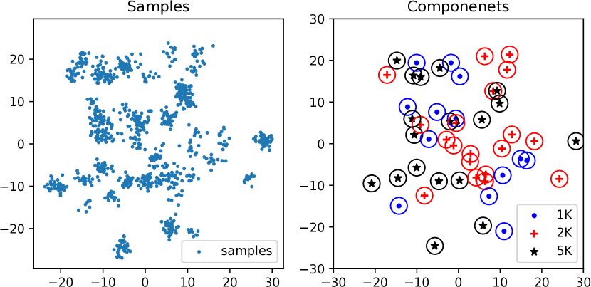
The synthetic dataset is for studying the behavior of the proposed method. It comprises $141K$ two-dimensional points from $50$ Gaussian components with unit variance. The sizes of clusters range from $1000$ to $5000$ to emulate the unbalanced settings that often occur in practice. Figure 1 shows the data set. We can observe overlaps among clusters, which makes the estimation nontrivial.

The ImageNet dataset is constructed from the training set of ILSVRC Russakovsky et al. (2015), which comprises $1.28M$ images in $1000$ categories. We extract a $2048$-dimensional feature for each image with Inception-ResNet Szegedy et al. (2016) and reduce the dimension to $48$ by PCA. Note that our purpose is to investigate mixture modeling instead of striving for top classification performance. Hence, it is reasonable to reduce the feature dimension to a moderate level, as samples are too sparse to form clusters in a very high dimensional space. We formulate a Gaussian mixture to describe the feature samples, where the covariance of each Gaussian components is fixed to $\sigma^{2}I$ with $\sigma=8$. We use $\mathcal{N}(0,\sigma_{0}^{2}I)$ as the prior distribution over the mean parameters of these components, where $\sigma_{0}=8$.

For the New York Time (NYT) Corpus Sandhaus (2008), we construct a vocabulary with $9866$ distinct words, and derive a bag-of-word representation for each article. Removing those with less than $20$ words, we obtain a data set with about $1.7M$ articles. We use a mixture of multinomial distribution to describe the NYT corpus. The prior here is a symmetric Dirichlet distribution with hyperparameter $\gamma=1$.

Figure 1: Visualization of the synthetic data set

Experiment Settings.

We compared eight methods. Four baselines: CGS - Collapsed Gibbs sampling Neal (2000), SliceMR - Map-reduce slice sampler Ge et al. (2015), AV - Auxiliary variable parallel Gibbs sampler Williamson et al. (2013) , and SubC - Parallel sampler via sub-cluster splits Chang and Fisher III (2013). Three different configurations of the proposed method: Prog - Synchronous Progressive consolidation (Sec 4.2), Pooled - Synchronous Pooled consolidation (Sec 4.2), and Async - Asynchronous consolidation (Sec 4.3). And Hung - we replace our consolidation step with Hungarian algorithm, which was adopted for component identification in Campbell et al. (2015).

These algorithms were examined from different aspects, including convergence, clustering accuracy, communication cost, and scalability. Each algorithm was launched for $10$ times (with different random seeds) on all data sets. We report the average of the performance metrics. We conducted the experiments using up to $30$ workers on multiple physical servers. They can communicate with each other via Gigabit Ethernet or TCP loop-back interfaces.

Figure 2: Log-likelihood w.r.t.iteration and runtime

Convergence.

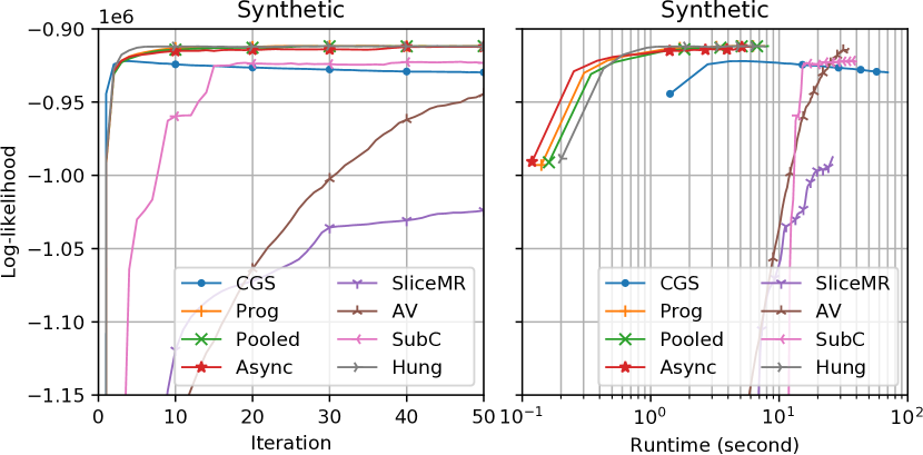
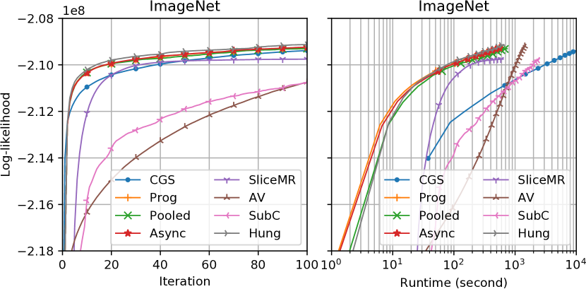
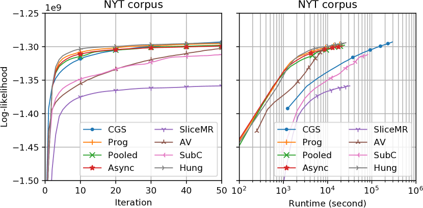
We first compare the convergence of the log-likelihood. Results on all three datasets are shown in Figure 2, where the likelihoods are plotted as functions of the number of iterations or the wall-clock time.

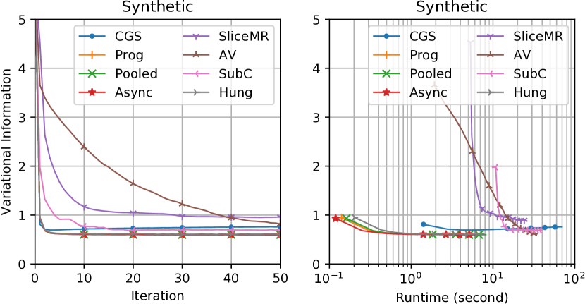
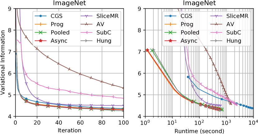
We observe that our algorithms can converge to the same level as CGS within comparable numbers of iterations on all three datasets, but are about $10$ to $20$ times faster owing to concurrency. On the synthetic dataset, we noticed that CGS yields small noisy clusters, which slightly decreased the likelihood. While in our algorithms, such clusters will be merged via consolidation, thus resulting in slightly higher likelihood. Overall, our methods achieve high scalability without compromising the convergence performance.

Other baseline methods designed for parallel estimation, namely SliceMR, AV and SubC, usually take more iterations and thus longer runtime to converge. Particularly, in SliceMR, new components are created from the prior distribution without reference to the data. Consequently, these new components are likely to be poor fits to the observed data. This has also been observed by Ge et al. (2015). In AV, large numbers of similar clusters will be proposed from different workers. However, placement of clusters is random instead of based on similarity. Therefore, it usually takes multiple iterations for all similar clusters to meet at a same worker and be merged. AV is fast on NTY dataset because each worker hold only a small portion of components due to sample movement, but many of them cannot be effectively merged. As a result, it results in more than 500 components, while this number is about 160 for our methods and 60 for SliceMR. In SubC, new components are generated only in the global split steps. Hence, more iterations are required to generate enough components to fit the data. Hung performs the same or even a little better than our methods when compared w.r.t.iterations. However, when compared w.r.t.runtime, this variant takes 5% to 10% longer to converge to the same level of log-likelihood. Because it involves a relatively more expensive procedure.

Figure 3: VI w.r.t.iteration and runtime

Clustering Performance.

An important application of mixture modeling is to discover clusters in exploratory data analysis. Following this practical standpoint, we also tested all algorithms on the first two dataset with provided ground-truths. Particularly, clustering performance is measured in terms of the Variation Information (VI) Meilă (2003) between the inferred sample assignments and the ground-truths. We show the performance metric against both the number of iterations and the clock time in Figure 3. Again, compared to CGS, our methods also achieve the same or even better performance with the same number of iterations, while taking drastically shorter (about $1/10$ of the CGS runtime on the synthetic dataset, and about $1/20$ on ImageNet). Hung performs similar as compared to our methods. SliceMR, AV and SubC can also achieve reasonable level of VI on both data sets, but it takes considerably longer.

Communication Cost.

Communication cost is crucial in distributed computing, especially when the bandwidth is limited. We evaluate the communication cost by measuring the number of bytes communicated and the number of communication times within each iteration, as shown in Table 1. Since out methods and Hung share the same communication policy, we merge them to one column and fill their the average value in the table.

	Ours / Hung	SliceMR	AV	SubC
#KBytes	50.7	40.9	4819.7	2320.4
#Times	40	40	114.6	40

(a) Synthetic dataset

	Ours / Hung	SliceMR	AV	SubC
#MBytes	6.01	4.89	49.9	26.2
#Times	40	40	114	40

(b) ImageNet dataset

Table 1: Communication cost

Our methods and SliceMR require minimal communication. In our algorithm, each worker communicates with the master by only two times in each iteration and the amount of data transfer is proportional to the number of cluster and the size of sufficient statistics only. SliceMR behaves similarly in this respect – it only communicates twice per iteration, transferring only the statistics. On the contrary, AV requires moving clusters among processors in the global MCMC steps. SubC require moving both the labels and the sufficient statistics to the master for splitting. Thus these two methods require much higher communication costs.

Figure 4: Speed up ratio

Scalability.

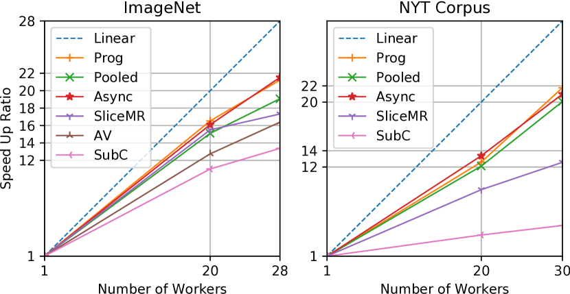
To study the scalability, we calculated the speed-up ratio w.r.t. CGS for each tested algorithm. As Figure 4 shows, both our Prog and Async algorithms achieve high scalability, while the scalability of Pooled is little bit lower. This is expected – our Prog algorithm involves only lightweight global merge steps while Pooled has a heavier MCMC step. In the Async algorithm, consolidation is performed concurrently with local inferences, thus Async can achieve very high scalability as Prog. The scalability of AV and SubC is considerably poorer, as moving data and label among workers poses significant communication overhead. Moreover, the unbalanced workload among processors Gal and Ghahramani (2014) also contributes to the poor scalability of AV. Note that the high scalability of SliceMR is at the expense of the convergence performance. Whereas it achieves nearly $21\times$ speed up w.r.t. its own runtime with a single worker, the overall performance still leaves a lot to be desired due to slow convergence (i.e. taking many more iterations than CGS).

6 Conclusions

We presented a new method for distributed estimation of DPMMs that can work under both synchronous and asynchronous settings. The method allows workers to perform local updates and create new components independently through delayed synchronization, while effectively tackling the issue of component identification via consolidation. Experimental results on both synthetic and real-world data clearly show that this method can achieve high scalability without compromising the convergence rate.

References

- Antoniak [1974] Charles E Antoniak. Mixtures of dirichlet processes with applications to bayesian nonparametric problems. The annals of statistics, pages 1152–1174, 1974.
- Blei and Jordan [2005] David M. Blei and Michael I. Jordan. Variational inference for dirichlet process mixtures. Bayesian Analysis, 1:121–144, 2005.
- Blei et al. [2003] David M Blei, Andrew Y Ng, and Michael I Jordan. Latent dirichlet allocation. Journal of machine Learning research, 3(Jan):993–1022, 2003.
- Blei [2016] David M Blei. The exponential family. 2016.
- Campbell et al. [2015] Trevor Campbell, Julian Straub, John W Fisher III, and Jonathan P How. Streaming, distributed variational inference for bayesian nonparametrics. In Advances in Neural Information Processing Systems, pages 280–288, 2015.
- Chang and Fisher III [2013] Jason Chang and John W Fisher III. Parallel sampling of dp mixture models using sub-cluster splits. In Advances in Neural Information Processing Systems, pages 620–628, 2013.
- Gal and Ghahramani [2014] Yarin Gal and Zoubin Ghahramani. Pitfalls in the use of parallel inference for the dirichlet process. In Proceedings of the 31st International Conference on Machine Learning (ICML-14), pages 208–216, 2014.
- Ge et al. [2015] Hong Ge, Yutian Chen, Moquan Wan, and Zoubin Ghahramani. Distributed inference for dirichlet process mixture models. In Proceedings of the 32nd International Conference on Machine Learning (ICML-15), pages 2276–2284, 2015.
- Jain and Neal [2004] Sonia Jain and Radford M Neal. A split-merge markov chain monte carlo procedure for the dirichlet process mixture model. Journal of Computational and Graphical Statistics, 13(1):158–182, 2004.
- Lin et al. [2010] Dahua Lin, Eric Grimson, and John Fisher. Construction of dependent dirichlet processes based on poisson processes. In Proceedings of the 23rd International Conference on Neural Information Processing Systems, pages 1396–1404. Curran Associates Inc., 2010.
- MacEachern and Müller [1998] Steven N MacEachern and Peter Müller. Estimating mixture of dirichlet process models. Journal of Computational and Graphical Statistics, 7(2):223–238, 1998.
- Meilă [2003] Marina Meilă. Comparing clusterings by the variation of information. In Learning theory and kernel machines, pages 173–187. Springer, 2003.
- Neal [2000] Radford M Neal. Markov chain sampling methods for dirichlet process mixture models. Journal of computational and graphical statistics, 9(2):249–265, 2000.
- Newman et al. [2007] David Newman, Padhraic Smyth, Max Welling, and Arthur U Asuncion. Distributed inference for latent dirichlet allocation. In Advances in neural information processing systems, pages 1081–1088, 2007.
- Newman et al. [2009] David Newman, Arthur Asuncion, Padhraic Smyth, and Max Welling. Distributed algorithms for topic models. The Journal of Machine Learning Research, 10:1801–1828, 2009.
- Russakovsky et al. [2015] Olga Russakovsky, Jia Deng, Hao Su, Jonathan Krause, Sanjeev Satheesh, Sean Ma, Zhiheng Huang, Andrej Karpathy, Aditya Khosla, Michael Bernstein, Alexander C. Berg, and Li Fei-Fei. ImageNet Large Scale Visual Recognition Challenge. International Journal of Computer Vision (IJCV), 115(3):211–252, 2015.
- Sandhaus [2008] Evan Sandhaus. The new york times annotated corpus. Linguistic Data Consortium, Philadelphia, 6(12):e26752, 2008.
- Sethuraman [1994] Jayaram Sethuraman. A constructive definition of dirichlet priors. Statistica sinica, pages 639–650, 1994.
- Smyth et al. [2009] Padhraic Smyth, Max Welling, and Arthur U Asuncion. Asynchronous distributed learning of topic models. In Advances in Neural Information Processing Systems, pages 81–88, 2009.
- Szegedy et al. [2016] Christian Szegedy, Sergey Ioffe, and Vincent Vanhoucke. Inception-v4, inception-resnet and the impact of residual connections on learning. CoRR, abs/1602.07261, 2016.
- Walker [2007] Stephen G Walker. Sampling the dirichlet mixture model with slices. Communications in Statistics—Simulation and Computation®, 36(1):45–54, 2007.
- Williamson et al. [2013] Sinead Williamson, Avinava Dubey, and Eric Xing. Parallel markov chain monte carlo for nonparametric mixture models. In Proceedings of the 30th International Conference on Machine Learning, pages 98–106, 2013.