The Critical Radius in Sampling-based Motion Planning
Abstract
We develop a new analysis of sampling-based motion planning in Euclidean space with uniform random sampling, which significantly improves upon the celebrated result of Karaman and Frazzoli (2011) and subsequent work. Particularly, we prove the existence of a critical connection radius proportional to for samples and dimensions: Below this value the planner is guaranteed to fail (similarly shown by the aforementioned work, ibid.). More importantly, for larger radius values the planner is asymptotically (near-)optimal. Furthermore, our analysis yields an explicit lower bound of on the probability of success. A practical implication of our work is that asymptotic (near-)optimality is achieved when each sample is connected to only neighbors. This is in stark contrast to previous work which requires connections, that are induced by a radius of order . Our analysis is not restricted to PRM and applies to a variety of “PRM-based” planners, including RRG, FMT∗ and BTT. Continuum percolation plays an important role in our proofs. Lastly, we develop similar theory for all the aforementioned planners when constructed with deterministic samples, which are then sparsified in a randomized fashion. We believe that this new model, and its analysis, is interesting in its own right.
1 Introduction
Motion planning is a fundamental problem in robotics concerned with allowing autonomous robots to efficiently navigate in environments cluttered with obstacles. Although motion planning has originated as a strictly theoretical problem in computer science [18], nowadays it is applied in various fields. Notably, motion planning arises in coordination of multiple autonomous vehicles [12], steering surgical needles [5], and planning trajectories of spacecrafts in orbit [47], to name just a few examples.
Motion planning is notoriously challenging from a computational perspective due to the continuous and high-dimensional search space it induces, which accounts for the structure of the robot, the physical constraints that it needs to satisfy, and the environment in which it operates. Low-dimensional instances of the problem can typically be solved by efficient and complete algorithms [17], and the same applies to several high-dimensional instances (see, e.g., [1, 44]). However, in general, motion planning is computationally intractable (see, e.g., [7, 35, 42]).
Nowadays the majority of practical approaches for motion planning capture the connectivity of the free space by sampling (typically in a randomized fashion) configurations and connecting nearby samples, to form a graph data structure. Although such sampling-based planners are inherently incomplete, i.e., cannot detect situations in which a solution (collision-free path) does not exist, most have the desired property of being able to find a solution eventually, if one exists. That is, a planner is probabilistically complete (PC) if the probability of finding a solution tends to as the number of samples tends to infinity. Moreover, some recent sampling-based techniques are also guaranteed to return high-quality solutions that tend to the optimum as diverges—a property called asymptotic optimality (AO). Quality can be measured in terms of energy, length of the plan, clearance from obstacles, etc.
An important attribute of sampling-based planners, which dictates both the running time and the quality of the returned solution, is the number of neighbors considered for connection for each added sample. In many techniques this number is directly affected by a connection radius : Decreasing reduces the number of neighbors. This in turn reduces the running time of the planner for a given number of samples , but may also reduce the quality of the solution or its availability altogether. Thus, it is desirable to come up with a radius that is small, but not to the extent that the planner loses its favorable properties of PC and AO.
1.1 Contribution
We develop a new analysis of PRM [24] for uniform random sampling in Euclidean space, which relies on a novel connection between sampling-based planners and continuum percolation (see, e.g., [11]). Our analysis is tight and proves the existence of a critical connection radius , where is a constant (in particular, for all ), and is the dimension: If then PRM is guaranteed to fail, where is the dimension. Above the threshold, i.e., when , PRM is AO for the bottleneck cost, and asymptotically near optimal333AnO means that the cost of the solution tends to at most a constant factor times the optimum, compared with AO in which this constant is equal to one. (AnO) with respect to the path-length cost. Furthermore, our analysis yields concrete bounds on the probability of success, which is lower-bounded by . Notice that this bound is comparable to the one obtained in [48] (see Section 2) although we show this for a much smaller radius.
Our analysis is not restricted to PRM and applies to a variety of planners that maintain PRM-like roadmaps, explicitly or implicitly. For instance, when is above the threshold, FMT∗ [21] is AnO with respect to the path-length cost, while BTT [43] is AO with respect to the bottleneck cost. RRG [23] behaves similarly for the two cost functions. Our results are also applicable to multi-robot motion planners such as the recently introduced dRRT∗ [10], and M∗ [51] when applied to a continuous domain. See Figure 1 for additional PRM-based planners to which our analysis is applicable, and which are mentioned further on.
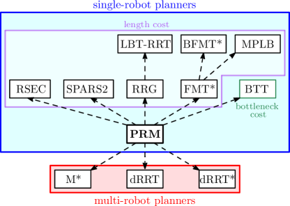
A practical implication of our work is that AO (or AnO), under the regime of uniform random sampling, can be achieved even when every sample is connected to neighbors. This is in stark contrast with previous work, e.g., [21, 23, 41, 45], which provided a rough estimate of this number, that is proportional to . Interestingly, our bound for uniform samples is comparable to the best known bound of for deterministic samples [22].
Lastly, we also study the asymptotic properties of the aforementioned planners when constructed using a deterministic point process, rather than uniform random sampling which we have mentioned so far. We introduce an analysis which shows that the graphs constructed using such deterministic samples can be sparsified in a randomized fashion while maintaining AO or AnO of the planners. We term this regime as semi-deterministic sampling.
1.2 Organization
In Section 2 we discuss related work. Then we proceed to basic definitions and problem statement in Section 3. In that section we also include a precise description of the robotic system our theory is developed for. Our central contribution (Theorem 1), which states the existence of a critical radius with respect to PRM, is presented in Section 4. This section also contains an outline of the proof. In Section 5 we lay the foundations of the proof and discuss important aspects of continuum percolation, that would later be employed in the main proof, which appears in Section 6. In Section 7 we extend the analysis to FMT∗, BTT, RRG and discuss the implications of our results to the multi-robot planners dRRT∗ and M∗. In Section 8 we present experimental work, which validates our theory. We conclude this paper with directions for future work (Section 9).
In the appendix we include proofs that were omitted from the main document and a table with values of . We also present in the appendix a new analysis for the aforementioned planners when constructed with deterministic samples, which are then sparsified in a randomized fashion. We believe that this new model, and its analysis, is interesting in its own right.
2 Related work
This section is devoted to a literature review of sampling-based planners with emphasis on their theoretical analysis. Sampling-based techniques were first described in the mid 90’s and several prominent examples of that time, that are still used extensively today, include PRM [24], RRT [29], and EST [20]. Those planners are also known to be PC (see [25, 28, 27, 20]).
More recent work has been concerned with the quality of the returned solution. [32] were one of the first to address this matter in a mathematically-rigorous manner. This work proved that RRT can produce arbitrarily-bad (long) paths with non-negligible probability.
The influential work of [23] laid the theoretical foundations for analyzing quality in sampling-based planning. The authors introduced a set of techniques to prove AO. Using their framework, they showed that the following algorithms are AO: PRM∗, which is a special case of PRM (throughout this work we will refer to the more general algorithm PRM rather than PRM∗) with a specific value of the connection radius ; an AO variant of RRT [29] termed RRT∗; RRG, which can be viewed as a combination between RRT and PRM. The analysis in [23] establishes that guarantees AO, where the configuration space of the robot is assumed to be . This indicates that the expected number of neighbors used per vertex should be . The authors also proved that for sufficiently-small radii of order the planner is guaranteed to fail (asymptotically) in finding any solution.
Following the breakthrough of [23], other AO planners have emerged (see e.g., [2, 4, 14]). [21] introduced FMT∗, which is a single-query planner that traverses an implicitly-represented PRM graph, and is comparable in performance to RRT∗. The authors refined the proof technique of [23], which allowed them to slightly reduce the connection radius necessary to FMT∗ and PRM to achieve AO. We do mention that here again . BFMT∗, which is a bidirectional version of FMT∗, was introduced by [48]. In this paper the authors also proved that the success rate of PRM, FMT∗, BFMT∗ can be lower bounded by , where is a tuning parameter. In this context, we also mention the work of [9], which bounds the success rate with an expression that depends on the amount of deviation from the optimum.
A recent work by [45] developed a different method for analyzing sampling-based planners. It exploits a connection with random geometric graphs (RGGs), which have been extensively studied (see, e.g., [33]). Their work shows that one can slightly reduce the PRM and FMT∗ radius obtained in [21]. Furthermore, the connection with RGGs yields additional analyses of different extensions of PRM, which have not been analyzed before in a mathematically-rigorous setting.
A number of methods have been developed to reduce the running time or space requirements of existing planners by relaxing AO constraints to AnO. For instance, LBT-RRT [37] interpolates between the quick RRT and the AO yet slower RRG, according to a predefined parameter. MPLB [36] can be viewed as a relaxation of FMT∗. SPARS2 [8] and RSEC [38] perform a sparsification of PRM in an online or offline fashion, respectively, to reduce the space footprint of the produced roadmap.
2.1 Extensions
The aforementioned papers deal mainly with the cost function of path length. Two recent works [41, 43] considered the bottleneck-pathfinding problem in a sampling-based setting and introduced the BTT algorithm, which traverses an implicitly-represented PRM graph. The bottleneck-cost function, which arises for instance in high-clearance multi-robot motion [43] and Fréchet matching between curves [19], is defined as follows: Every robot configuration is paired with a value , and the cost of a path is the maximum value of along any configuration on the path. It was shown [41, 43] that BTT is AO, with respect to bottleneck cost, for the reduced connection radius that was obtained by [45].
The results reported until this point have dealt exclusively with holonomic robotic systems. Two recent papers by [39, 40] develop the theoretical foundations of PRM and FMT∗-flavored planners when applied to robots having differential constraints. [30] develop an AO algorithm that does not require a steering function, as PRM for instance does. Interestingly, the authors of the last paper also obtain bounds on the rate of convergence of their algorithm.
3 Preliminaries
We provide several basic definitions that will be used throughout the paper. Given two points , denote by the standard Euclidean distance. Denote by the -dimensional ball of radius centered at and for any . Similarly, given a curve define . Given a subset we denote by its Lebesgue measure. All logarithms are at base .
3.1 Motion planning
Denote by the configuration space of the robot, and by the free space, i.e., the set of all collision free configurations. Though our proofs may be extended to more complex robotic systems (see discussion in Section 9), in this work we investigate the geometric (holonomic) setting of the problem in which no constraints are imposed on the motion of the robot. Additionally, we assume that is some subset of the Euclidean space. In particular, for some fixed . We also assume that for any two configurations the robot is capable of following precisely the straight-line path from to .
Given start and target configurations , the problem consists of finding a continuous path (curve) such that . That is, the robot starts its motion along on , and ends in , while remaining collision free. An instance of the problem is defined for a given , where .
3.2 Cost function
It is usually desirable to obtain paths that minimize a given criterion. In this paper we consider the following two cost functions.
Definition 1.
Given a path , its length is
Definition 2.
Given a path , and a cost map , its bottleneck cost is
We proceed to describe the notion of robustness, which is essential when discussing properties of sampling-based planners. Given a subset and two configurations , denote by the set of all continuous paths, whose image is in , that start in and end in , i.e., if then and .
Definition 3.
Let be a motion-planning problem. A path is robust if there exists such that . We also say that is robustly feasible if there exists such a robust path.
Definition 4.
The robust optimum with respect to is defined as
The corresponding definition for the bottleneck cost is slightly more involved.
Definition 5.
Let be a cost map. A path is -robust if it is robust and for every there exists such that for every , . We also say that is well behaved if there exists at least one -robust path.
Definition 6.
The robust optimum with respect to is defined as
3.3 Poisson point processes
We draw our main analysis techniques from the literature of continuum percolation, where point samples are generated with the following distribution. Thus we will use this point distribution in PRM, which would be formally defined in the following section.
Definition 7 ([11]).
A random set of points is a Poisson point process (PPP) of density if it satisfies the conditions:
-
1.
For mutually disjoint domains , the random variables are mutually independent.
-
2.
For any bounded domain we have that for every ,
Informally, property (1) states that the number of points from in any two disjoint sets is independent. Another useful property that follows from (2) is that the expected number of points in a certain region is known precisely and corresponds to the volume of this region. That is, for any it holds that .
The following provides a simple recipe for generating PPP.
Claim 1 ([11]).
Let be a Poisson random variable with mean . For a given draw a sample and define to be points chosen independently and uniformly at random from . Then is a PPP of density .
It will be convenient to think about PRM as a subset of the following random geometric graph (RGG). We will describe various properties of this graph in later sections.
Definition 8.
[33] Let be a PPP. Given , the random geometric graph is an undirected graph with the vertex set . Given two vertices , if .
4 Analysis of PRM
In this section we provide a mathematical description of PRM, which essentially maintains an underlying RGG with PPP samples. We proceed to describe our main contribution (Theorem 1) which is concerned with the conditions for which PRM converges to the (robust) optimum. We then provide an outline of the proof, in preparation for the following sections.
Recall that the configuration space of the robot is represented by , and the free space is denoted by . The motion-planning problem will remain fixed throughout this section.
Recall that PRM accepts as parameters the number of samples and a connection radius . Denote by a PPP with mean density . In relation to the definitions of the previous section, the graph data structure obtained by the preprocessing stage of PRM can be viewed as an RGG. For instance, when , the graph obtained by PRM is precisely . In the more general case, when , PRM produces the graph . As can be non-convex, we emphasize that the latter notation describes the maximal subgraph of such that vertices and edges are contained in .
In the query stage, recall that PRM accepts two configurations , which are then connected to the preprocessed graph. Here we slightly diverge from the standard definition of PRM in the literature. In particular, instead of using the same radius when connecting , we use the (possibly larger) radius . The graph obtained after query is formally defined below:
Definition 9.
The PRM graph is the union between and the supplementary edges
Remark. We emphasize that the larger radius is only used when are connected to the preprocessed RGG.
We reach our main contribution.
Theorem 1.
Suppose that is robustly feasible. Then there exists a critical radius , where is a constant (see supplementary material), such that the following holds:
-
i.
If and then PRM fails (to find a solution) a.a.s. 444Let be random variables in some probability space and let be an event depending on . We say that occurs asymptotically almost surely (a.a.s., in short) if .
-
ii.
Suppose that . There exists such that for , where , and any the following holds with probability :
-
1.
contains a path with , where is independent of ;
-
2.
If is well behaved then contains a path with .
-
1.
Remark: Theorem 1 also holds, with a slight modification, when the PPP is replaced with the standard binomial point process (BPP), in which the number of sampled points is fixed a priori. The only difference is that the probability of success should be reduced from to . This follows from Lemma 1 in [13], which states that if a property holds for PPP then it also holds for BPP, albeit with slightly smaller probability.
4.1 Outline of proof
For the remainder of this section we briefly describe our technique for proving this theorem, in preparation for the full proof, which is given in Section 6. The critical radius defined above, coincides with the percolation threshold, which determines the emergence of a connected component of that is of infinite size. In particular, if then breaks into tiny connected components of size each. Thus, unless are infinitesimally close, no connected component can have both and simultaneously.
More interestingly, the radius of leads to the emergence of a unique infinite component of . That is, in such a case one of the components of must contain an infinite number of vertices (Section 5.1). Denote this component by .
In contrast to , which is defined for the unbounded space , our motion-planning problem is bounded to . Thus, the next step is to investigate the properties of when restricted to (Section 5.2). Denote by the largest connected component of . This structure plays a key role in our proof (see Section 6): With high probability (to be defined), there exist vertices of that are sufficiently close to and , respectively, so that a connection between the two vertices can be made through .
Of course, this overlooks the fact that some portions of lie in forbidden regions of . Thus, we also have to take the structure of into consideration. To do so, we rely on [34] to prove that any small subset of must contain at least one point of (see lemmata 2 and 3). This allows us to trace the robust optimum (and collision-free) path with points from .
The final ingredient, which allows to bound the path length along , is Theorem 4. It states that the distance over this graph is proportional to the Euclidean distance between the end points. This also ensures that the trace points from can be connected with collision-free paths over the graph.
5 Elements of continuum percolation
In this section we describe some of the properties of the unbounded graph that will be employed in our analysis in the following section.
5.1 The basics
A fundamental question is when contains an infinite connected component around the origin.
Definition 10.
The percolation probability is the probability that the origin is contained in a connected component of of an infinite number of vertices. That is, if denotes the set of vertices connected to in the graph, then .
We say that a graph percolates iff . Note that the selection of the origin is arbitrary, and the following result can be obtained for any alternative to .
Theorem 2.
[16, Theorem 12.35] There exists a critical radius , where is a constant, such that when , and when .
The following lemma states that the infinite connected component exists with probability strictly or .
Lemma 1.
Let be the probability that contains an infinite connected component, i.e., without conditioning on any specific additional vertex. Then when and when .
Proof.
Suppose that , and for any , denote by the percolation probability of , and note that . Define , and observe that for any there exists such that . By definition, percolates, i.e., the infinite component touches , iff there exists such that . By definition of , if the latter event occurs then there exists such that . Thus, by applying the union bound, and noting that a sum of countable number of zeros is still zero, we establish that
For the other direction we employ Kolmogorov’s zero-one law (see, e.g., [6, Theorem 1, p.36]). Informally, it states that an event, e.g., existence of an infinite connected component in , that occurs independently of any finite subset of independent random variables, e.g., points from , has a ability of either or . Thus, as it immedietly follows that when . ∎
The following theorem establishes that the infinite connected component is unique.
Theorem 3.
[31, Theorem 2.3] With probability , contains at most one infinite connected component.
5.2 Bounded domains
We study different properties of when it is restricted to the domain . In case that , we use to refer to the infinite connected component of the unbounded graph . Note that exists (Lemma 1) and is unique (Theorem 3) with probability .
Denote by the largest connected component of . By definition, is also a subgraph of . The following lemma shows that with high probability all the points from , that are sufficiently close to the center of , are members of .
Lemma 2.
Let . Define
Denote by the event that . Then there exist and such that for any it holds that
Proof.
This statement is an adaptation of Lemma 8 and Theorem 2 of [34]. We mention that [34] uses a slightly different, but nevertheless equivalent model. While we consider an RGG that is bounded to and PPP of density , they consider the domain with density . It is only a matter of rescaling and variable substitution to import their results to our domain. Let denote the connected components of , and set to be the component with the largest number of vertices. Without loss of generality, . See illustration in Figure 2.
Observe that if then it must have at least one vertex that lies closely to the boundary of , i.e., , as otherwise will not be able to connect to the rest of . Thus, it must be the case that in order to be able to reach , where defines the diameter of a given . We shall show that this does not hold.
Theorem 2 in [34] states that for any large enough there exist such that for any it holds with probability at least that for any . By setting the conclusion immediately follows. ∎
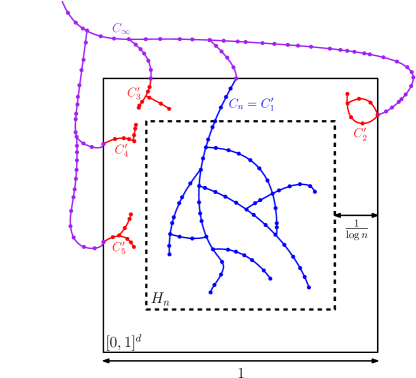
Observe that for any fixed point internal to there exists such that for any it holds that . The following lemma bounds the probability of having at least one point from in a (small) subregion of . Note that the value corresponds to the value used in Theorem 1.
Lemma 3.
Let . Define to be a hypercube of side length
Denote by the event that . Then there exists and such that for any it holds that .
Proof.
Define , and observe that .
We treat as a subset of in order to apply a rescaling argument. Observe that (scalar) multiplication of every point of with yields a translation of . We will use the superscript to describe this rescaling to a given object. For instance, applying the same transformation on yields the graph , which has the same topology as . Denote by the (lexicographically) smallest point of , i.e., . Notice that
where the minus sign in the left-hand side represents a translation by a vector. This implies that , which is defined over behaves as . This allows to leverage Theorem 1 from [34], which bounds the number of vertices from the unbounded component. In particular, there exists such that
While this is an overkill for our purpose, it does the job in proving that . As we assume that holds (Lemma 2), it follows that holds with probability at least . ∎
The following statement allows to bound the graph distance between two connected vertices. We endow every edge of the graph with a length attribute that represents the Euclidean distance between the edges’ endpoints. For every two vertices of , denotes the length of the shortest (weighted) path on between the two vertices.
Theorem 4.
[13, Theorem 3] Let . There exists a constant , independent of , such that , where the event is defined as follows: For any two vertices in the same connected component of , with , it holds that .
6 Proof of Theorem 1
Proofs for all the three settings of the main theorem are given individually in the subsections below.
6.1 Case i
Here we provide proof for the first (and easy) part of the theorem, which states that PRM fails when , even with . We mention that our proof is a simpler and shorter version of a similar proof that was given in [23] for a slightly different setting.
We show below that in the subcritical regime, i.e., , the graph breaks into many small connected components. In particular, the probability of having the largest connected component of size decays exponentially in . Denote by the size of the largest connected component in .
Proposition 1.
Let . Then a.a.s.
Proof.
First, we start by stating that there exist a constant and an integer such that for all it holds that . This is a simplified version of Proposition 11.2 in [33], which is given for uniformly sampled points, to the case of PPP, which we have here. In particular, the original proof relies on a relation between these two distributions, which transforms uniform sampling into a PPP and induces an additional factor that is not necessary in our setting. In particular, the factor “” which appears in Equation 11.1 in [33] should be eliminated.
To conclude the proof, we set , where , similarly to the proof of Theorem 11.1, Equation 11.4 in [33]. Observe that as tends to . ∎
Now, consider the configuration space depicted in Figure 3 (similar examples can be devised for any ). The white and blue regions represent the free space. Observe that any path connecting to must go through the blue region, whose width is greater than . Also note that any point contained in the blue region cannot be connected by an edge from or , which deems the large value of as irrelevant.
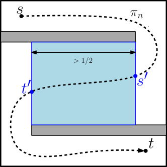
Suppose that contains a path (black dashed curve) connecting and , and denote by the subpath that is contained in the blue region. Also, denote by and the first and last points along , respectively. Obviously . Then, the number of edges of , which induce , is at least . However, this is in contradiction with the fact that every connected component of is of logarithmic size in (Proposition 1).
6.2 Case ii.1
We provide a full proof for the positive setting with length cost. The proof for the bottleneck case, which appears later on, is very similar to the length case.
Suppose that , . For simplicity, we set , where . By Lemma 1 and Theorem 3, contains a unique infinite connected component . Recall that denotes the largest connected component of . Also note that , where is defined in Lemma 3.
Recall that denotes the robust optimum, with respect to path length (Definition 4). Fix . By definition, there exists a robust path and such that and . See illustration in Figure 4.
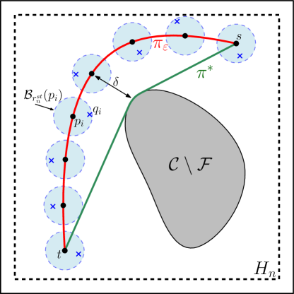
We now define a sequence of points along that are separated by exactly units, where is as defined in Theorem 4. In particular, define , set , and assign along , such that , where represents the subpath of starting at and ending at . Notice that is finite.
Claim 2.
Proof.
Define to represent a -dimensional (axis-aligned) hypercube of side length that is centered in . Formally, . Observe that for large enough. Also note that . Thus, the result follows from the union bound. ∎
Suppose that are satisfied. Let be the points obtained from Claim 2. These points reside in a single connected component of . Define the path
where represents a straight-line path from to , and represents the shortest path from to in . The next claim states that if in addition is satisfied (Theorem 4), then is also collision free.
Claim 3.
Suppose that are satisfied. Then is a path in (with probability ).
Proof.
First, observe that the straight-line paths are contained in due to the definition of PRM and the fact that . Let us consider a specific subpath . Recall from Claim 2 and by definition of that , which is bounded by . Thus, for any point along it holds that . Thus, . ∎
The next claim states that the length of is a constant factor from the optimum.
Claim 4.
Suppose that are satisfied. We have that (with probability ).
Proof.
First, observe that by the triangle inequality, it holds that
By Theorem 4 and the triangle inequality, it follows that
We note that in order to eliminate the summand one can fix but work with instead of , where . For simplicity, we chose to leave the proof as is. ∎
6.3 Case ii.2
We prove the asymptotic optimality of PRM for bottleneck cost, with appropriate values of . The proof follows very similar lines to that of the length cost. Fix . For simplicity we assume that (the proof can be adapted to larger values of ). By definition, there exists an -robust path and such that
-
(a)
,
-
(b)
,
-
(c)
and .
Now, define . By substituting with , and with in the proof of Theorem 1.ii, it follows that if are satisfied, contains a path such that . This implies that
which concludes this proof.
7 Analysis of other planners
In this section we describe the implications of Theorem 1 to additional planners, which are closely related to PRM. In all the results below, the values are identical to those in Theorem 1. Furthermore, for simplicity of presentation, we assume that is robustly feasible, and is well behaved, where relevant.
We first consider FMT∗ and BTT, and then proceed to RRG, whose analysis is more involved. In all the following algorithms we assume that the sampling method is a PPP.
7.1 The FMT∗ and the BTT planners
The following two corollaries are direct consequences of Theorem 1 as the two algorithms FMT∗ and BTT traverse an implicitly-represented PRM graph while minimizing the cost functions and , respectively.
Corollary 1.
If and then FMT∗ fails a.a.s. If and , then for any FMT∗ returns a path with with probability .
We remark that FMT∗ can ignore certain edges of the underlying PRM graph, which may result in a path of lower quality than that obtained by PRM. However, this situation only occurs for vertices which lie within distance of from (see [21, Remark 3.3]). As our analysis of PRM in the previous section utilizes only vertices and edges that are far from obstacles our proofs extend to FMT∗ straightforwardly.
Corollary 2.
If and then BTT fails a.a.s. If and , then for any BTT returns a path with with probability .
7.2 The RRG planner
We consider the incremental planner RRG, which can be viewed as a cross between RRT and PRM. Due to this relation we can extend the analysis of PRM to RRG. (The term “incremental” refers to planners that generate samples one after the other, and connect the current samples to previous ones.)
We introduce an incremental version of a PPP to extend our theory to RRG.
Claim 5.
Let be a Poisson random variable with mean . At each iteration draw a sample and define to be points chosen independently and uniformly at random from . The set , obtained after iterations, is a PPP of density .
Note that the sum of i.i.d. Poisson random variables with means is a Poisson random variable with mean . Claim 5 follows directly from this property.
We now describe an adaptation of RRG for an incremental PPP. Given a start configuration and a goal region , RRG initializes a roadmap with a single node . Let denote the constant used by RRG for local steering (see [23]). Similarly to PRM, RRG employs the connection radii .
Let be a Poisson random variable with mean and let denote the number of nodes of the constructed roadmap after iterations. At the th iteration we draw a sample and define to be points chosen independently and uniformly at random from . RRG will iteratively process the samples , as follows: For a sample RRG will first locate the nearest node to . Let be a node at distance at most from at the direction of . RRG will attempt to connect to . If the connection attempt is successful, the new node will be added to the roadmap. Then, RRG will attempt to connect to all the existing nodes within a ball of radius . It will additionally attempt to connect to if . Note that for the th iteration of RRG we set .
The connection radii that will be used during the th iteration are fixed, as both are functions of the number of nodes in the roadmap at the beginning of the iteration. Both radii will be set to decrease with the number of roadmap nodes, as in PRM. However, since we fix the radius at each iteration of RRG we use a slightly larger radius than the one obtained had we considered the current roadmap size. This will clearly keep all relevant connections and perhaps even add more.
Theorem 5.
Suppose that is robustly feasible (we extend Definition 3 to describe a robustly feasible path for RRG). Let denote the roadmap constructed by RRG after iterations with
where are as in Theorem 1.ii, and is any positive constant. Then for any the following holds with probability :
-
1.
contains a path with ;
-
2.
If is well behaved then, contains a path with .
7.2.1 Proof of Theorem 5
We provide proof only for , as the case for is almost identical. In what follows we consider a robust path for which . Let denote the clearance of , and denote its length. Finally, set .
Our proof uses Theorem 1 as a central ingredient, due to the following observation, which is formalized below: For large enough, with probability , contains a PRM roadmap in the vicinity of , where is slightly smaller than . This in turn follows from the unique structure of RRG, which can be viewed as a combination of PRM and RRT, as RRG supplements the RRT tree with additional edges.
In particular, the following corollary can be deduced from the probabilistic completeness of RRT with samples from a PPP (see Appendix B), which does not rely on the parameters .
Claim 6.
It is possible to tile with balls of radius , such that after iterations of RRG, with probability at least for some constants , every ball will contain at least one RRG vertex.
The following lemma formalizes the connection between RRG and PRM.
Lemma 4.
Fix and define . Let be an RRG graph constructed after iterations with connection radii . With probability at least , for some constants , the graph contains a PRM graph , constructed with the radius .
Proof.
Consider the first iterations of RRG. From Claim 6 we obtain that given a robust path , it can be tiled using a constant number of balls of radius such that with probability of at least every ball will contain an RRG vertex after iterations of RRG, for some constants , and . Now, let us consider a new sample that is added in iteration . By Claim 6, includes (with certain probability) a node that can be connected to ; that is, both and the straight-line path from to is collision free. Thus, is a added as a node to RRG and then connected in a PRM-fashion to all its neighbors within a radius of .
Note that the smallest value of the latter radius is when . Observe that
Additionally,
This implies that all samples added after iteration are connected in a PRM-fashion with a radius . Thus, contains a PRM graph , constructed with the radius with probability , as required. ∎
We are now ready to finish the proof of Theorem 5. Let us denote by the event that the graph contains a PRM graph . Given that occurs, we denote by the event that the constructed roadmap maintains the good properties of PRM, as defined in Theorem 1.ii.1. That is, contains a path with ;
Given that occurs, from Theorem 1 we obtain that occurs on the PRM-like graph inside with probability of at least
That is, . Additionally, Lemma 4 states that for some . Note that we would like to bound the probability that both and occur simultaneously. From the definition of conditional probability we have that . Therefore,
7.3 Multi-robot planners
In this section we briefly state the implications of our analysis of PRM for sampling-based multi-robot motion planning. In particular, we consider the planners M∗ [51], dRRT [46] and dRRT∗ [10].
The multi-robot setting involves robots operating in a shared workspace. In this more challenging setting collisions between different robots must be avoided, in addition to standard robot-obstacle collisions. Single-robot sampling-based planners can be applied directly to the problem by considering the robot fleet as one highly-complex robot. However, recently-introduced planners that are tailored for the multi-robot case have proved to be much more effective than the aforementioned naive approach.
Such recent approaches include M∗, dRRT, and dRRT∗. A common ground to these techniques is an implicit construction of a composite roadmap [46], which results from a tensor product between single-robot roadmaps —for every the graph is a PRM embedded in the configuration space of robot . It was recently proved that if are AO, with respect to the individual robots for which they are defined, then is AO with respect to the multi-robot problem [10].
Thus, by Theorem 1 it follows that the underlying single-robot PRM graphs can be constructed using a smaller connection radius, while still guaranteeing the AO (or AnO) of . This in turn, guarantees AO (or AnO) of M∗, dRRT∗, and PC of dRRT.
8 Experimental results
We present experiments demonstrating the effect of using different values of the connection radius on the running time, cost of solution for the length cost , and success rate, when running the algorithms PRM and FMT∗ on problems of dimensions up to . In particular, ranges between the critical radius (Theorem 1) and previously obtained upper bounds from [21, 23].
We validate our theory for PRM (Theorem1) and FMT∗ (Corollary 1). We observe that smaller connection radii, than previously-obtained bounds, still allow the planners to converge to high-quality, near-optimal paths. Furthermore, we identify situations in which using a radius that is close to allows to obtain a high-quality solution more quickly. Moreover, although the resulting cost for the smaller radii can be slightly worse, we observe that postprocessing the paths using standard simplification methods yields solutions that are only marginally inferior to the best (postprocessed) solution. Specifically, in harder scenarios the advantage in using a smaller connection radius is more prominent; in some cases we obtain a reduction of 50% in running time, with an improved cost, and similar success rates when compared to the results obtained using the original FMT∗ connection radius.
8.1 Implementation details
In our experiments, we used the Open Motion Planning Library (OMPL 1.3, [49]) on a 2.6GHz Intel Core i5 processor with 16GB of memory. Results were averaged over 50 runs and computed for dimensions up to 12.
The planners that we used are PRM and the batch variant of FMT∗, which were adapted for samples from a PPP, where is the expected number of samples. Specifically, given the expected number of samples , these variants generate a set of samples according to the recipe in Claim 1. The two planners use the connection radii . Note that should be at least , but the exact value of is unknown. For simplicity, we set to be identical to , defined in [23]. We emphasize that although we use an asymptotically smaller value, it still yields (empirically) convergence in cost. This suggests that the bound on can be further reduced.
![[Uncaptioned image]](/html/1709.06290/assets/x5.png)
Given a scenario and a value , we define a set of increasing connection radii, , as follows. We set the minimal connection radius to be , where . Note that is larger than by a factor of roughly . The maximal connection radius, denoted by , is as defined in [21]. For each we define , where . Now, for every scenario and number of samples we run our planning algorithm with , and . Note that all our plots are for , and that in some experiments an additional radius appears as well (see [23]). The figure to the right depicts the colors and labeling that will be used throughout this section.
8.2 Results
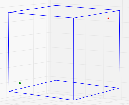
Euclidean space. The scenario we consider (see Figure 5(a)) consists of a point robot moving in the obstacle-free unit -dimensional hypercube. Therefore, . We set the start and target positions of the robot to be and , respectively.
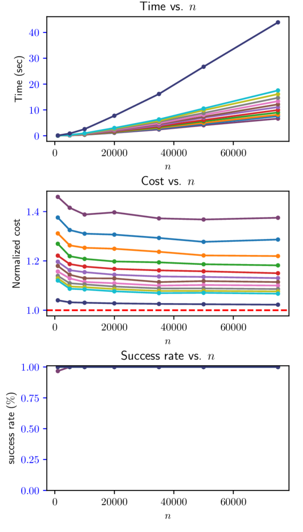
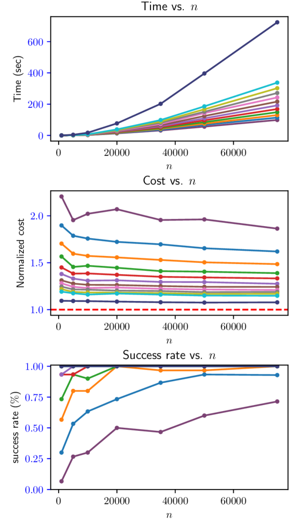
We run PRM and plot (i) the overall running time, (ii) the normalized cost () of the obtained solution, where a value of 1 represents the best possible cost, and (iii) the portion of successful runs—all as a function of the expected number of samples . Results are depicted in Figure 6.
The plots demonstrate the following trend: for each radius the cost obtained by PRM converges to some constant times the optimal cost, which is marked with the dashed red curve in the “Cost vs. ” plot. (We note that it is possible that for larger values of the cost values for different radii will eventually converge to the same value.) Clearly, yields the best cost but at the price of increased running time. obtains the next best cost, with improved running time, and so on. Note that for , already for K a solution is found for all radii except , whereas for and K a solution is found for all radii above . It is important to note that there is a clear speedup in the running times of PRM when using for , over , with a slight penalty (a factor of roughly ) in the resulting costs.
For the first set of experiments of PRM in an obstacle free -dimensional hypercube, we also study how the value of affects the size of the connected components. Note that Theorem 1 in [34] states that . In particular, we measure the size of the two largest connected components, denoted by and , as a function of both the radius and the expected number of samples . The results for are summarized in Table 1. Already for , is significantly larger than . However, for there is no clear difference. That is, we do not see in practice the expected emergence of the “huge” component. As increases, the proportion of increases as well, whereas that of shrinks. Also note that for specific the maximal component is smaller for than for .
| 2 | 1K | 0.17 | 0.1 | 0.88 | 0.05 | 1.0 | 0.0 |
|---|---|---|---|---|---|---|---|
| 2 | 5K | 0.08 | 0.05 | 0.97 | 0.001 | 0.999 | 0.0 |
| 2 | 10K | 0.05 | 0.04 | 0.98 | 0.003 | 1.0 | 0.0 |
| 2 | 50K | 0.02 | 0.01 | 0.99 | 0.001 | 1.0 | 0.0 |
| 12 | 1K | 0.04 | 0.02 | 0.84 | 0.003 | 1.0 | 0.0 |
| 12 | 5K | 0.12 | 0.01 | 0.91 | 0.001 | 1.0 | 0.0 |
| 12 | 10K | 0.21 | 0.005 | 0.94 | 0.001 | 1.0 | 0.0 |
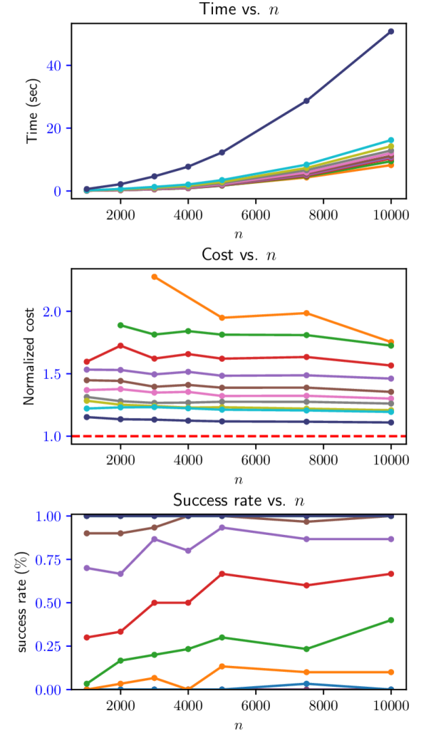
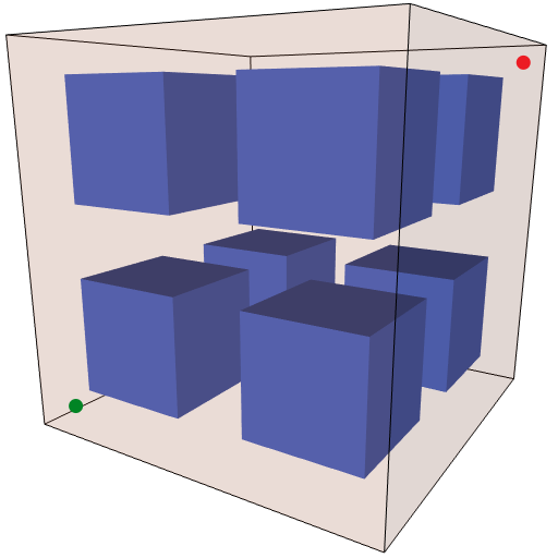
General Euclidean space. We consider the following -dimensional scenario (based on a scenario from [45]), for , depicted in Figure 5(b) in 3D, and a point robot: is subdivided into sub-cubes by halving it along each axis. Each sub-cube contains a centered -dimensional axis-aligned hypercubical obstacle that covers 25% of the sub-cube. The start position of the robot is placed on the diagonal between and , such that it is equidistant from the origin and from the closest hypercubical obstacle. is selected similarly, with respect to .
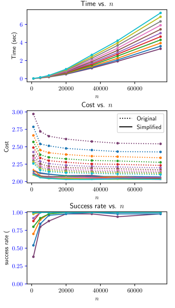
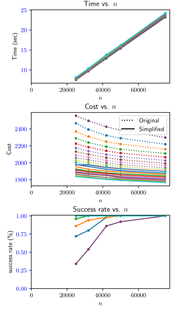
Here we use FMT∗ with radii ranging from to . We also ran PRM which exhibited a similar behavior. Figure 7(a) presents the results for . We plot the average cost after simplifying the resulting paths in addition to the average original cost. We mention that there is a difference in cost between the various radii and that costs obtained using larger radii are often better. However, after applying OMPL’s default path-simplification procedure we obtain paths with negligible differences in cost. This suggests that paths obtained using the smaller connection radii are of the same homotopy class as the path obtained using .
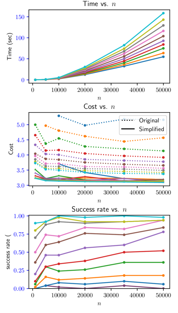
For (Figure 7(b)), as in the case of , costs obtained using larger radii are often better. However, applying OMPL’s default path-simplification procedure yields paths with negligible differences in cost. We do mention, though, that the success rates of all radii deteriorate, when compared to .
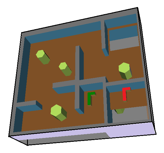
General non-Euclidean space. We use the Cubicles scenario (see Figure 5(c)) provided with the OMPL distribution [49]. Here the goal is to find a collision-free path for one or two L-shaped robots that need to exchange their positions. In the single-robot case, the robot needs to move between the two configurations depicted in red and green. In the two-robot case, these two configurations represent the start positions of the robots, where the goal is for each robot to finish at the start of the other robot. Since the robots are allowed to translate and rotate, then or , respectively, and is non-Euclidean. Although our theory does not directly apply here, we chose to test it empirically for such a setting.
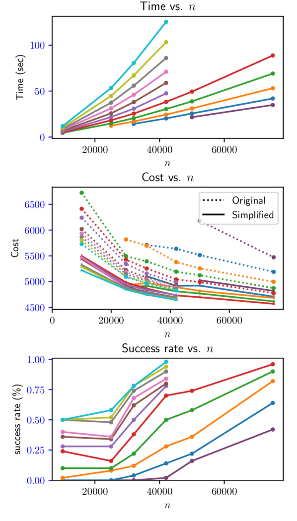
We ran our experiments with FMT∗ using a connection radii ranging from to . Initially, no solution was found in all runs. Indeed, as was mentioned in [26], this is not surprising, since the theory from which the radius values are derived assumes that the configuration space is Euclidean. In the same paper the authors propose a heuristic for effectively using radius-based connections in motion planning. In our experiments (Figure 8(b)) we increased all radii by a multiplicative factor of and , respectively, in order to increase the success rates. We mention that this yielded similar behavior to that when using the connection scheme suggested in [26].
Results for the single-robot case are depicted in 8(a). In this case, even with 25K samples already with (green) we were able to obtain high successes rates. The running time was slightly better than that of , whereas the cost was higher than the one obtained using . However, after applying the smoothing procedure the difference in cost decreased significantly.
Let us proceed to the two-robot setting. Observe in Figure 8(b), that the variance in cost after path simplification is again significantly smaller than the variance in the original cost. Clearly, smaller radii exhibit shorter running times, but with smaller success rates. However, since the success rate improves as the number of samples increases, one could use the smaller radii with larger and still obtain a solution with comparable cost and success rate in shorter running time. Indeed, using (green) with 75K samples we obtain a solution whose cost (after simplification) is slightly better than the cost obtained using with 42K samples (after simplification). Moreover, the running time of the former is roughly 50% of the time taken for the latter, and both obtain similar success rates. This indicates that in such settings, one could benefit from using smaller radii in terms of favorable running times and obtain a comparable or even better cost with similar success rates.
9 Future work
In this work we leveraged techniques from percolation theory to develop stronger analysis of PRM-based sampling-based motion planners. In the hope of providing mathematically rigorous presentation, while still being accessible, we chose to focus the discussion on simplified, possibly unrealistic, robotic systems. In particular, we assumed a holonomic system having a Euclidean configuration space.
Our immediate future goal is to extend our theory to non-Euclidean spaces, such as those arising from rigid bodies translating and rotating in space. The next challenge will be to extend the model to robots with differential constraints. While the latter task seems daunting, we should keep in mind that the state space of such systems can be modeled as a differential manifold. This may allow to locally apply our Euclidean-space techniques to analyze manifold spaces. Indeed, a similar approach has already been considered in previous work [39, 40].
The next algorithmic challenge is to consider robotic systems for which precise steering, i.e., solving the two-point boundary value problem, cannot be performed, at least not efficiently (see discussion in [30, Section 1.3]). In such cases, PRM-based planners (as we considered here), or RRT∗-based techniques, cannot be applied. We pose the following question: Is it possible to extend existing planners to work in the absence of a steering function, while maintaining their theoretical properties? We plan to tackle this question in the near future.
10 Acknowledgments
We thank the participants of the Workshop on Random Geometric Graphs and Their Applications to Complex Networks, 2015, and in particular Carl P. Dettmann, Mathew Penrose, Paul Balister, and Yuval Peres, for fruitful discussions. We also thank Dan Halperin for commenting on early drafts of the paper.
This work has been supported in part by the Israel Science Foundation (grant no. 825/15), by the Blavatnik Computer Science Research Fund, and by the Blavatnik Interdisciplinary Cyber Research Center at Tel Aviv University. M.K. is supported in part by the Yandex Foundation. This work was prepared as part of K.S.’s Ph.D. thesis in Tel Aviv University, with the support of the Clore Israel Foundation.
Appendix
Appendix A Theory for (semi-)deterministic sampling
So far we have studied the theoretical properties of various sampling-based planners constructed with the PPP sample set . In this section we study similar aspects but for a different sampling regime. Particularly, we replace with which represents a rectilinear lattice, also known as a Sukharev sequence. A recent paper by [22] studies the theoretical properties of PRM and FMT∗ when constructed with (and other deterministic low-dispersion sequences). Here we introduce a new analysis which shows that PRM constructed with can be further sparsified while maintaining AO. This result can also be extended to FMT∗, BTT, RRG and other planners, as was done in Section 7 for the setting of PPP.
A.1 The basics
We start with some basic definitions. For a given define and . That is, contains all the points of a rectangular lattice, with edge length . Observe that is a deterministic graph which connects by an edge every two points that differ in exactly one coordinate and the distance between them is exactly . We proceed to define a randomized subset of :
Definition 11.
Given , the graph is defined in the following manner. Every point of is added independently with probability to as a vertex. Two vertices are connected by an edge if .
This corresponds to a well-studied model of site percolation. Similarly to the continuous model studied in the previous section, we say that percolates if it contains an infinite connected component that includes the origin . Also denote by the largest connected component of .
The following theorem corresponds to a combination of Theorem 2, Lemma 1, and Theorem 3 for the continuous case.
Theorem 6.
[11] There exists a critical value such that for the graph percolates with probability zero. If then percolates with non-zero probability. Furthermore, if then is unique with probability .
The next two lemmata serve as discrete versions of Lemma 2 and Lemma 3, respectively. Their proofs are very similar to the original proofs and are therefore omitted. We do mention that they rely on Theorem 5 and Theorem 4 of [34], respectively.
Lemma 5.
Suppose that . Denote by the event that , where is as defined in Lemma 2. Then there exists and such that for any it holds that
Lemma 6.
Suppose that . Define to be a hypercube of side length
Denote by the event that . Then there exist and such that for any it holds that .
Now we proceed to the discrete counterpart of Theorem 4. For any define . The following is a simplified version of [3, Theorem 1.1].
Theorem 7.
Suppose that . There exists a positive constant such that for any two fixed points it holds that
For the subcritical regime (), we have the following theorem. Define
That is, represents all the points in that can be reached from by at most edges of length over the corresponding rectilinear lattice. Denote by the boundary of , i.e., all the points that are exactly edges from . Let be the event that contains a path from to some vertex in .
Theorem 8.
([16, Theorem 5.4]) If , there exists a constant such that for all .
This theorem implies that in the subcritical regime it is improbable that has a path connecting two lattice points as defined above, as such a path must have edges.
A.2 Back to motion planning
To conclude this section, we define a sparsified version of PRM defined on the deterministic samples , and state its theoretical properties. The proof is omitted as it is almost identical to the one obtained in Section 4, with the difference that it now uses theorems and lemmata presented earlier this section, rather than the ones from Section 5.
Recall that PRM uses the two connection radii . For simplicity we fix .
Definition 12.
The sparsified PRM graph is the union between and the supplementary edges
Theorem 9.
Suppose that is robustly feasible. Then there exists such that the following holds:
-
i.
If and then PRM fails (to find a solution) a.a.s.
-
ii.
Suppose that . There exists such that for , where , and any the following holds a.a.s.:
-
1.
contains a path with ;
-
2.
If is well behaved then, contains a path with .
-
1.
Appendix B Probabilistic completeness of RRT with samples from a PPP
This section is devoted to the proof of Claim 6. A probabilistic completeness proof of RRT, for the setting of uniform random sampling, is given in [27, Section 3]. We describe here how to modify this proof for samples from a PPP, which are of interest in the present paper.
Note that RRT is an incremental planning algorithm, which generates samples one after the other, and connects the current sample to previous ones. Therefore, it should employ the incremental PPP sampling defined in Claim 5.
We wish to apply the line of arguments as for the uniform-sampling case described in [27, Theorem 1]. This theorem assumes that a path from start to target exists, whose clearance is and length is . The path is covered with a set of balls of radius , where and is a constant depending on both the steering parameter of RRT and the clearance . The proof describes the process as a Markov chain with transition probability , where is the probability to produce an RRT vertex in the st ball given that there exists an RRT vertex in the th ball . It then shows that the probability that RRT will not produce samples within all balls decays to zero exponentially as the number of samples tends to infinity. To adapt the proof for samples from a PPP, it suffices to outline how to compute the transition probability ,
Recall that at each iteration we draw a sample , where is a Poisson random variable with mean , and define to be points chosen independently and uniformly at random from . Let denote the event that , and let denote the event that at least one of falls inside . Since , we will bound . Observe that
and note that . Therefore,
Appendix C Critical values
In this section we provide for reference a list of (estimates) of the values and .
C.1 Continuum percolation
Table 2 presents an estimate of such that percolates only if , for . It is directly derived from [50, Table I], where an estimate of the critical node degree is derived. We mention that for large enough [50], where is volume of the Lebesgue measure of the unit ball in .
C.2 Lattice percolation
Table 3 presents the value of for , the best known estimates for . Numbers in round brackets are single standard deviations.
References
- Adler et al. [2015] Aviv Adler, Mark de Berg, Dan Halperin, and Kiril Solovey. Efficient multi-robot motion planning for unlabeled discs in simple polygons. IEEE Trans. Automation Science and Engineering, 12(4):1309–1317, 2015.
- Alterovitz et al. [2011] Ron Alterovitz, Sachin Patil, and Anna Derbakova. Rapidly-exploring roadmaps: Weighing exploration vs. refinement in optimal motion planning. In IEEE International Conference on Robotics and Automation (ICRA), pages 3706–3712, 2011.
- Antal and Pisztora [1996] Peter Antal and Agoston Pisztora. On the chemical distance for supercritical bernoulli percolation. The Annals of Probability, 24(2):1036–1048, 1996.
- Arslan and Tsiotras [2013] Oktay Arslan and Panagiotis Tsiotras. Use of relaxation methods in sampling-based algorithms for optimal motion planning. In IEEE International Conference on Robotics and Automation (ICRA), pages 2413–2420, 2013.
- Baykal and Alterovitz [2017] Cenk Baykal and Ron Alterovitz. Asymptotically optimal design of piecewise cylindrical robots using motion planning. In Robotics: Science and Systems, 2017.
- Bollobás and Riordan [2006] Bela Bollobás and Oliver Riordan. Percolation. Cambridge University Press, 2006.
- Canny [1988] John Canny. The complexity of robot motion planning. MIT press, 1988.
- Dobson and Bekris [2014] Andrew Dobson and Kostas E. Bekris. Sparse roadmap spanners for asymptotically near-optimal motion planning. International Journal of Robotics Research, 33(1):18–47, 2014.
- Dobson et al. [2015] Andrew Dobson, George V. Moustakides, and Kostas E. Bekris. Geometric probability results for bounding path quality in sampling-based roadmaps after finite computation. In IEEE International Conference on Robotics and Automation, pages 4180–4186, 2015.
- Dobson et al. [2017] Andrew Dobson, Kiril Solovey, Rahul Shome, Dan Halperin, and Kostas E. Bekris. Scalable asymptotically-optimal multi-robot motion planning. In International Symposium on Multi-Robot and Multi-Agent Systems, 2017.
- Franceschetti and Meester [2008] Massimo Franceschetti and Ronald Meester. Random Networks for Communication: From Statistical Physics to Information Systems. Cambridge Series in Statistical and Probabilistic Mathematics. Cambridge University Press, 2008.
- Frazzoli and Pavone [2013] Emilio Frazzoli and Marco Pavone. Multi-vehicle routing. In John Baillieul and Tariq Samad, editors, Encyclopedia of Systems and Control, pages 1–11. Springer London, 2013.
- Friedrich et al. [2013] Tobias Friedrich, Thomas Sauerwald, and Alexandre Stauffer. Diameter and broadcast time of random geometric graphs in arbitrary dimensions. Algorithmica, 67(1):65–88, 2013.
- Gammell et al. [2015] Jonathan D. Gammell, Siddhartha S. Srinivasa, and Timothy D. Barfoot. Batch informed trees (BIT*): Sampling-based optimal planning via the heuristically guided search of implicit random geometric graphs. In IEEE International Conference on Robotics and Automation (ICRA), pages 3067–3074, 2015.
- Grassberger [2003] Peter Grassberger. Critical percolation in high dimensions. Phys. Rev. E, 67:036101, Mar 2003.
- Grimmett [1999] Geoffrey R. Grimmett. Percolation, volume 321 of Comprehesive Studies in Mathematics. Springer, 1999.
- Halperin et al. [2016a] Dan Halperin, Lydia Kavraki, and Kiril Solovey. Robotics. In Jacob E. Goodman, Joseph O’Rourke, and Csaba D. Toth, editors, Handbook of Discrete and Computational Geometry, chapter 51. CRC Press LLC, 3rd edition, 2016a. URL \urlhttp://www.csun.edu/ ctoth/Handbook/HDCG3.html.
- Halperin et al. [2016b] Dan Halperin, Oren Salzman, and Micha Sharir. Algorithmic motion planning. In Jacob E. Goodman, Joseph O’Rourke, and Csaba D. Toth, editors, Handbook of Discrete and Computational Geometry, chapter 50. CRC Press LLC, 3rd edition, 2016b. URL \urlhttp://www.csun.edu/ ctoth/Handbook/HDCG3.html.
- Holladay et al. [2017] Rachel M. Holladay, Oren Salzman, and Siddhartha Srinivasa. Minimizing task space frechet error via efficient incremental graph search. CoRR, abs/1710.06738, 2017. URL \urlhttp://arxiv.org/abs/1710.06738.
- Hsu et al. [1999] David Hsu, Jean-Claude Latombe, and Rajeev Motwani. Path planning in expansive configuration spaces. International Journal of Computational Geometry and Applications, 9(4/5), 1999.
- Janson et al. [2015] Lucas Janson, Edward Schmerling, Ashley A. Clark, and Marco Pavone. Fast marching tree: A fast marching sampling-based method for optimal motion planning in many dimensions. International Journal of Robotics Research, 34(7):883–921, 2015.
- Janson et al. [2017] Lucas Janson, Brian Ichter, and Marco Pavone. Deterministic sampling-based motion planning: Optimality, complexity, and performance. International Journal of Robotics Research, 2017.
- Karaman and Frazzoli [2011] Sertac Karaman and Emillio Frazzoli. Sampling-based algorithms for optimal motion planning. International Journal of Robotics Research, 30(7):846–894, 2011.
- Kavraki et al. [1996] Lydia E. Kavraki, Petr Svestka, Jean-Claude Latombe, and Mark Overmars. Probabilistic roadmaps for path planning in high dimensional configuration spaces. IEEE Transactions on Robotics and Automation, 12(4):566–580, 1996.
- Kavraki et al. [1998] Lydia E. Kavraki, Mihail N. Kolountzakis, and Jean-Claude Latombe. Analysis of probabilistic roadmaps for path planning. IEEE Trans. Robotics and Automation, 14(1):166–171, 1998.
- Kleinbort et al. [2016] Michal Kleinbort, Oren Salzman, and Dan Halperin. Collision detection or nearest-neighbor search? On the computational bottleneck in sampling-based motion planning. In International Workshop on the Algorithmic Foundations of Robotics (WAFR), 2016.
- Kleinbort et al. [2018] Michal Kleinbort, Kiril Solovey, Zakary Littlefield, Kostas E. Bekris, and Dan Halperin. Probabilistic completeness of RRT for geometric and kinodynamic planning with forward propagation. IEEE Robotics and Automation Letters, 2018. To appear.
- Ladd and Kavraki [2004] Andrew M. Ladd and Lydia E. Kavraki. Measure theoretic analysis of probabilistic path planning. IEEE Trans. Robotics and Automation, 20(2):229–242, 2004.
- LaValle and Kuffner Jr. [2001] Steven M. LaValle and James J. Kuffner Jr. Randomized kinodynamic planning. I. J. Robotics Res., 20(5):378–400, 2001.
- Li et al. [2016] Yanbo Li, Zakary Littlefield, and Kostas E. Bekris. Asymptotically optimal sampling-based kinodynamic planning. I. J. Robotics Res., 35(5):528–564, 2016.
- Meester and Roy [1994] Ronald Meester and Rahul Roy. Uniqueness of unbounded occupied and vacant components in boolean models. The Annals of Applied Probability, 4(3):933–951, 1994.
- Nechushtan et al. [2010] Oren Nechushtan, Barak Raveh, and Dan Halperin. Sampling-diagram automata: A tool for analyzing path quality in tree planners. In International Workshop on the Algorithmic Foundations of Robotics (WAFR), pages 285–301, 2010.
- Penrose [2003] Mathew D. Penrose. Random geometric graphs. Oxford University Press, 2003.
- Penrose and Pisztora [1996] Mathew D. Penrose and Agoston Pisztora. Large deviations for discrete and continuous percolation. Advances in Applied Probability, 28(1):29–52, 1996.
- Reif [1979] John H Reif. Complexity of the mover’s problem and generalization. In IEEE Symposium on Foundations of Computer Science (FOCS), pages 421–427, 1979.
- Salzman and Halperin [2015] Oren Salzman and Dan Halperin. Asymptotically-optimal motion planning using lower bounds on cost. In IEEE International Conference on Robotics and Automation (ICRA), pages 4167–4172, 2015.
- Salzman and Halperin [2016] Oren Salzman and Dan Halperin. Asymptotically near-optimal RRT for fast, high-quality motion planning. IEEE Trans. Robotics, 32(3):473–483, 2016.
- Salzman et al. [2014] Oren Salzman, Doron Shaharabani, Pankaj K. Agarwal, and Dan Halperin. Sparsification of motion-planning roadmaps by edge contraction. I. J. Robotics Res., 33(14):1711–1725, 2014.
- Schmerling et al. [2015a] Edward Schmerling, Lucas Janson, and Marco Pavone. Optimal sampling-based motion planning under differential constraints: The drift case with linear affine dynamics. In IEEE Conference on Decision and Control, pages 2574–2581, 2015a.
- Schmerling et al. [2015b] Edward Schmerling, Lucas Janson, and Marco Pavone. Optimal sampling-based motion planning under differential constraints: The driftless case. In IEEE International Conference on Robotics and Automation, pages 2368–2375, 2015b.
- Solovey and Halperin [2016a] Kiril Solovey and Dan Halperin. Sampling-based bottleneck pathfinding with applications to Fréchet matching. In European Symposium on Algorithms, pages 76:1–76:16, 2016a.
- Solovey and Halperin [2016b] Kiril Solovey and Dan Halperin. On the hardness of unlabeled multi-robot motion planning. I. J. Robotics Res., 35(14):1750–1759, 2016b.
- Solovey and Halperin [2017] Kiril Solovey and Dan Halperin. Efficient sampling-based bottleneck pathfinding over cost maps. In IEEE/RSJ International Conference on Intelligent Robots and Systems, 2017. to appear.
- Solovey et al. [2015] Kiril Solovey, Jingjin Yu, Or Zamir, and Dan Halperin. Motion planning for unlabeled discs with optimality guarantees. In Robotics: Science and Systems, 2015.
- Solovey et al. [2016a] Kiril Solovey, Oren Salzman, and Dan Halperin. New perspective on sampling-based motion planning via random geometric graphs. In Robotics: Science and Systems, 2016a.
- Solovey et al. [2016b] Kiril Solovey, Oren Salzman, and Dan Halperin. Finding a needle in an exponential haystack: Discrete RRT for exploration of implicit roadmaps in multi-robot motion planning. I. J. Robotics Res., 35(5):501–513, 2016b.
- Starek et al. [2016] J. A. Starek, E. Schmerling, G. D. Maher, B. W. Barbee, and M. Pavone. Real-time, propellant-optimized spacecraft motion planning under Clohessy-Wiltshire-Hill dynamics. In IEEE Aerospace Conference, Big Sky, Montana, 2016.
- Starek et al. [2015] Joseph A. Starek, Javier V. Gómez, Edward Schmerling, Lucas Janson, Luis Moreno, and Marco Pavone. An asymptotically-optimal sampling-based algorithm for Bi-directional motion planning. In IEEE/RSJ International Conference on Intelligent Robots and Systems, pages 2072–2078, 2015.
- Şucan et al. [2012] Ioan A. Şucan, Mark Moll, and Lydia E. Kavraki. The Open Motion Planning Library. IEEE Robotics & Automation Magazine, 19(4):72–82, 2012. \urlhttp://ompl.kavrakilab.org.
- Torquato and Jiao [2012] S. Torquato and Y. Jiao. Effect of dimensionality on the continuum percolation of overlapping hyperspheres and hypercubes. ii. simulation results and analyses. The Journal of Chemical Physics, 137(7):074106, 2012.
- Wagner and Choset [2015] Glenn Wagner and Howie Choset. Subdimensional expansion for multirobot path planning. Artif. Intell., 219:1–24, 2015.
- Wang et al. [2013] Junfeng Wang, Zongzheng Zhou, Wei Zhang, Timothy M. Garoni, and Youjin Deng. Bond and site percolation in three dimensions. Phys. Rev. E, 87:052107, May 2013.