N2N Learning: Network to Network Compression via Policy Gradient Reinforcement Learning
Abstract
While wider and deeper neural network architectures continue to advance the state-of-the-art for many computer vision tasks, real-world adoption of these networks is impeded by hardware and speed constraints. Conventional model compression methods attempt to address this problem by modifying the architecture manually or using pre-defined heuristics. Since the space of all reduced architectures is very large, modifying the architecture of a deep neural network in this way is a difficult task. In this paper, we tackle this issue by introducing a principled method for learning reduced network architectures in a data-driven way using reinforcement learning. Our approach takes a larger ‘teacher’ network as input and outputs a compressed ‘student’ network derived from the ‘teacher’ network. In the first stage of our method, a recurrent policy network aggressively removes layers from the large ‘teacher’ model. In the second stage, another recurrent policy network carefully reduces the size of each remaining layer. The resulting network is then evaluated to obtain a reward – a score based on the accuracy and compression of the network. Our approach uses this reward signal with policy gradients to train the policies to find a locally optimal student network. Our experiments show that we can achieve compression rates of more than for models such as ResNet-34 while maintaining similar performance to the input ‘teacher’ network. We also present a valuable transfer learning result which shows that policies which are pre-trained on smaller ‘teacher’ networks can be used to rapidly speed up training on larger ‘teacher’ networks.
1 Introduction
While carefully hand-designed deep convolutional networks continue to increase in size and in performance, they also require significant power, memory and computational resources, often to the point of prohibiting their deployment on smaller devices. As a result, researchers have developed model compression techniques based on Knowledge Distillation to compress a large (teacher) network to a smaller (student) network using various training techniques (e.g., soft output matching, hint layer matching, uncertainty modeling). Unfortunately, state-of-the-art knowledge distillation methods share a common feature: they require carefully hand-designed architectures for the student model. Hand-designing networks is a tedious sequential process, often loosely guided by a sequence of trial-and-error based decisions to identify a smaller network architecture. This process makes it very difficult to know if the resulting network is optimal. Clearly, there is a need to develop more principled methods of identifying optimal student architectures.
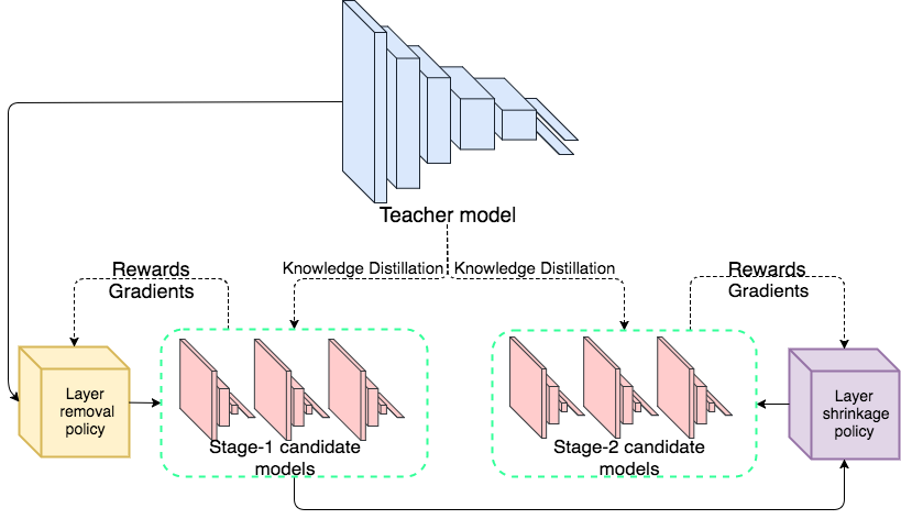
Towards a more principled approach to network architecture compression, we present a reinforcement learning approach to identify a compressed high-performance architecture (student) given knowledge distilled from a larger high-performing model (teacher). We make a key conceptual assumption that formulates the sequential process of converting a teacher network to a student network as a Markov Decision Process (MDP). Under this model, a state represents the network architecture. Clearly, the domain of the state is very large since it contains every possible reduced architecture of the teacher network. A deterministic transition in this state space, , is determined by selecting the action , e.g., removing a convolutional filter or reducing the size of a fully connected layer. Each action will transform one architecture to another architecture . Under the MDP, the strategy for selecting an action given a certain state is represented by the policy , which stochastically maps a state to an action. The process of reinforcement learning is used to learn an optimal policy based on a reward function defined over the state space. In our work, we define the reward function based on the accuracy and the compression rate of the specified architecture .
A straightforward application of reinforcement learning to this problem can be very slow depending on the definition of the action space. For example, an action could be defined as removing a single filter from every layer of a convolutional neural network. Since the search space is exponential in the size of the action space and sequence length, it certainly does not scale to modern networks that have hundreds of layers.
Our proposed approach addresses the problem of scalability in part, by introducing a two-stage action selection mechanism which first selects a macro-scale “layer removal” action, followed by a micro-scale “layer shrinkage” action. In this way we enable our reinforcement learning process to efficiently explore the space of reduced networks. Each network architecture that is generated by our policy is then trained with Knowledge Distillation Hinton et al. (2015). Figure 1 illustrates our proposed approach.
To the best of our knowledge, this is the first paper to provide a principled approach to the task of network compression, where the architecture of the student network is obtained via reinforcement learning. To facilitate reinforcement learning, we propose a reward function that encodes both the compression rate and the accuracy of the student model. In particular, we propose a novel formulation of the compression reward term based on a relaxation of a constrained optimization problem, which encodes the hardware-based computational budget items in the form of linear constraints.
We demonstrate the effectiveness of our approach over several network architectures and several visual learning tasks of varying difficulty (MNIST, SVHN, CIFAR-10, CIFAR-100, Caltech-256). We also demonstrate that the compression policies exhibit generalization across networks with similar architectures. In particular, we use a policy trained on a ResNet-18 model on a ResNet-34 model and show that it greatly accelerates the reinforcement learning process.
2 Related Work
We first discuss methods for compressing models to a manually designed network (pruning and distillation). Towards automation, we discuss methods for automatically constructing high-performance networks, orthogonal to the task of compression.
Pruning:
Pruning-based methods preserve the weights that matter most and remove the redundant weights LeCun et al. (1989), Hassibi et al. (1993), Srinivas & Babu (2015), Han et al. (2015b), Han et al. (2015a), Mariet & Sra (2015), Anwar et al. (2015), Guo et al. (2016). While pruning-based approaches typically operate on the weights of the teacher model, our approach operates on a much larger search space over both model weights and model architecture. Additionally, our method offers greater flexibility as it allows the enforcement of memory, inference time, power, or other hardware constraints. This allows our approach to find the optimal architecture for the given dataset and constraints instead of being limited to that of the original model.
Knowledge Distillation:
Knowledge distillation is the task of training a smaller network (a “student”) to mimic a “teacher” network, performing comparably to the input network (a “teacher”) Buciluǎ et al. (2006), Ba & Caruana (2014), Hinton et al. (2015), Romero et al. (2014), Urban et al. (2016). The work of Hinton et al. (2015) generalized this idea by training the student to learn from both the teacher and from the training data, demonstrating that this approach outperforms models trained using only training data. In Romero et al. (2014), the approach uses Knowledge Distillation with an intermediate hint layer to train a thinner but deeper student network containing fewer parameters to outperform the teacher network. In previous Knowledge Distillation approaches, the networks are hand designed, possibly after many rounds of trial-and-error. In this paper, we train a policy to learn the optimal student architecture, instead of hand-designing one. In a sense, we automate Knowledge Distillation, employing the distillation method of Ba & Caruana (2014) as a component of our learning process. In the experiments section we show that our learned architectures outperform those described in Romero et al. (2014) and Hinton et al. (2015).
Architecture Search:
There has been much work on exploring the design space of neural networks Saxe et al. (2011), Zoph & Le (2016), Baker et al. (2016), Ludermir et al. (2006), Miikkulainen et al. (2017), Real et al. (2017), Snoek et al. (2012), Snoek et al. (2015), Stanley & Miikkulainen (2002), Jozefowicz et al. (2015), Murdock et al. (2016), Feng & Darrell (2015), Warde-Farley et al. (2014), Iandola et al. (2016). The principal aim of previous work in architecture search has been to build models that maximize performance on a given dataset. On the other hand, our goal is to find a compressed architecture while maintaining reasonable performance on a given dataset. Our approach also differs from existing architecture search method since we use the teacher model as the search space for our architecture instead of constructing networks from scratch. Current methods that construct networks from scratch either operate on a very large search space, making it computationally expensive Zoph & Le (2016), Real et al. (2017), Miikkulainen et al. (2017), Jozefowicz et al. (2015) or operate on a highly restricted search space Baker et al. (2016), Snoek et al. (2015). Our approach instead leverages the idea that since the teacher model is able to achieve high accuracy on the dataset, it already contains the components required to solve the task well and therefore is a suitable search space for the compressed architecture.
3 Approach
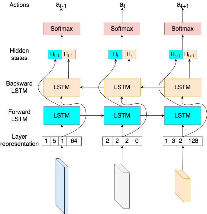
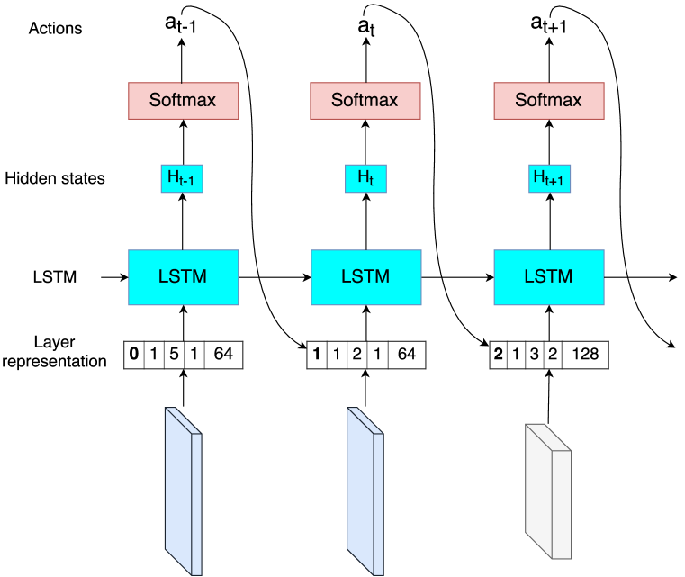
Our goal is to learn an optimal compression strategy (policy) via reinforcement learning, that takes a Teacher network as input and systematically reduces it to output a small Student network.
3.1 Markov Decision Process
We formulate the sequential process of finding a reduced architecture as a sequential decision making problem. The decision process is modeled as a Markov Decision Process (MDP). Formally, the MDP is defined as the tuple .
States: is the state space, a finite set consisting of all possible reduced network architectures that can be derived from the Teacher model. For example, a VGG network Simonyan & Zisserman (2014) represents the state (the initial state) and by removing one convolutional filter from the first layer we obtain a new network architecture .
Actions: is a finite set of actions that can transform one network architecture into another network architecture. In our approach there are two classes of action types: layer removal actions and layer parameter reduction actions. The definition of these actions are further described in Section 3.2.1 and 3.2.2.
Transition Function: is the state transition dynamic. Here, is deterministic since an action always transforms a network architecture to the resulting network architecture with probability one.
Discount Factor: is the discount factor. We use so that all rewards contribute equally to the final return.
Reward: is the reward function. The rewards of network architecture can be interpreted to be a score associated with a given network architecture . Note that we define the reward to be 0 for intermediate states, which represent “incomplete” networks, and only compute a non-trivial reward for the final state. The reward function is described in detail in Section 3.4.
3.2 Student-Teacher Reinforcement Learning
Under this MDP, the task of reinforcement learning is to learn an optimal policy , such that it maximizes the expected total reward, with the total reward given by:
| (1) |
We take a policy gradient reinforcement learning approach and iteratively update the policy based on sampled estimates of the reward. The design of the action space is critical for allowing the policy gradient method to effectively search the state space. If the actions are selected to be very incremental, a long sequence of actions would be needed to make a significant change to the network architecture, making credit assignment difficult. To address this issue, we propose a two stage reinforcement learning procedure. In the first stage a policy selects a sequence of actions deciding whether to keep or remove each layer of the teacher architecture. In the second stage, a different policy selects a sequence of discrete actions corresponding to the magnitude by which to attenuate configuration variables of each remaining layer. In this way, we are able to efficiently explore the state space to find the optimal student network.
A sketch of the algorithm is given in Algorithm 3.2. For both layer removal and shrinkage policies, we repeatedly sample architectures and update the policies based on the reward achieved by the architectures. We now describe the details of the two stages of student-teacher reinforcement learning.
3.2.1 Layer removal
In the layer removal stage, actions correspond to the binary decision to keep or remove a layer. The length of the trajectory for layer removal is , the number of layers in the network. At each step of layer removal, the Bidirectional LSTM policy (See Figure 2(a)) observes the hidden states, , as well as information about the current layer: . Information about the current layer is given as
where is the layer type, kernel size, stride, padding and number of outputs (filters or connections). To model more complex architectures, such as ResNet, and are used to inform the policy network about skip connections. For a layer inside a block containing a skip connection, is the number of layers prior to which the skip connection began and is the number of layers remaining until the end of the block. Additionally it is to be noted that although actions are stochastically sampled from the outputs at each time step, the hidden states that are passed on serve as a sufficient statistic for Wierstra et al. (2010).
3.2.2 Layer shrinkage
The length of the trajectory for layer shrinkage is , where is the number of configuration variables for each layer. At each step of layer shrinkage, the policy observes the hidden state , the previously sampled action and current layer information : . The parameterization of is similar to layer removal except that the previous action is appended to the representation in an autoregressive manner (See Figure 2(b)). The action space for layer shrinkage is defined as (each action corresponds to how much to shrink a layer parameter) and an action is produced for each configurable variable for each layer. Examples include kernel size, padding, and number of output filters or connections.
3.3 Reward function
The design of the reward function plays a critical role in learning the policies. A poorly designed reward that provides no discrimination between good and bad student architectures prevents policies from learning the trade-offs in architecture space. The objective of model compression is to maximize compression while maintaining a high accuracy. Since there is no benefit in producing highly compressed models which have bad performance, we want to provide a harsher penalty for a model with high compression + low accuracy than one with low compression + high accuracy. Furthermore we would also like to define a general reward function that does not depend on dataset/model specific hyperparameters. Additional discussion on the design of the reward function is provided in the appendix.
In our approach, we define the reward function as follows:
Where is the relative compression ratio of the student model, is the validation accuracy of the student model and is the validation accuracy of the teacher model provided defined as a constant. and refer to the compression and accuracy reward respectively. We compute the reward as a product of the compression and accuracy reward since we want the reward to scale with both quantities dependently. The compression reward, , is computed using a non-linear function that biases the policy towards producing models that maintain accuracy while optimizing for compression. The relative compression is defined in terms of the ratio of trainable parameters of each model: . It is noted here that other compression methods that use quantization or coding define compression ratio in terms of number of bits instead of parameters. The accuracy reward, , is defined with respect to the teacher model as , where refers to the validation accuracy of the student model and refers to the validation accuracy of the teacher model. We note that both accuracy and compression rewards are normalized with respect to the teacher and thus do not require additional hyperparameters to perform task-specific weighting. Lastly, it is possible that the policies may produce degenerate architectures in such cases, a reward if -1 is assigned (details in appendix).
3.3.1 Constraints as Rewards
Our approach allows us to incorporate pre-defined hardware or resource budget constraints by rewarding architectures that meet the constraints and discouraging those that do not. Formally, our constrained optimization problem is
where and form our constraints, and is vector of constrained variables. We relax these hard constraints by redefining our reward function as:
The introduction of the non-smooth penalty may result in a reduced exploration of the search space and hence convergence to a worse local minimum. To encourage early exploration gradually incorporate constraints over time:
where monotonically decreases with and . As it is possible to incorporate a variety of constraints such as memory, time, power, accuracy, label-wise accuracy, our method is flexible enough to produce models practically viable in a diversity of settings. This is in contrast to conventional model compression techniques which require many manual repetitions of the algorithm in order to find networks that meet the constraints as well as optimally balance the accuracy-size tradeoff.
3.4 Optimization
We now describe the optimization procedure for each our stochastic policies, and . The procedure is the same for each policy, thus we use in what follows. Each policy network is parameterized by its own .
Our objective function is the expected reward over all sequences of actions , i.e.:
We use the REINFORCE policy gradient algorithm from Williams Williams (1992) to train both of our policy networks.
where is the number of rollouts for a single gradient update, is the length of the trajectory, is the probability of selecting action given the hidden state , generated by the current stochastic policy parameterized by and is the reward of the rollout.
The above is an unbiased estimate of our gradient, but has high variance. A common trick is to use a state-independent baseline function to reduce the variance:
| (2) |
We use an exponential moving average of the previous rewards as the baseline . An Actor-Critic policy was also tested. While there was a minor improvement in stability, it failed to explore as effectively in some cases, resulting in a locally optimal solution. Details are in the appendix.
3.5 Knowledge distillation
Student models are trained using data labelled by a teacher model. Instead of using hard labels, we use the un-normalized log probability values (the logits) of the teacher model. Training using the logits helps to incorporate dark knowledge Hinton et al. (2015) that regularizes students by placing emphasis on the relationships learned by the teacher model across all of the outputs.
As in Ba & Caruana (2014), the student is trained to minimize the mean loss on the training data . Where are the logits of the teacher model.
where W represents the weights of the student network and is the model prediction on the training data sample.
Final student models were trained to convergence with hard and soft labels using the following loss function.
Where is the loss function used for training with hard labels (in our case cross-entropy) and are the ground truth labels.
| MNIST | |||||
| Architecture | Acc. | #Params | Acc. | Compr. | |
| VGG-13 | Teacher | 99.54% | 9.4M | — | — |
| Student (Stage1) | 99.55% | 73K | +0.01% | 127x | |
| CIFAR-10 | |||||
| VGG-19 | Teacher | 91.97% | 20.2M | — | — |
| Student (Stage1) | 92.05% | 1.7M | +0.08% | 11.8x | |
| Student (Stage1+Stage2) | 91.64% | 984K | -0.33% | 20.53x | |
| ResNet-18 | Teacher | 92.01% | 11.17M | — | — |
| Student (Stage1) | 91.97% | 2.12M | -0.04% | 5.26x | |
| Student (Stage1+Stage2) | 91.81% | 1.00M | -0.2% | 11.10x | |
| ResNet-34 | Teacher | 92.05% | 21.28M | — | — |
| Student (Stage1) | 93.54% | 3.87M | +1.49% | 5.5x | |
| Student (Stage1+Stage2) | 92.35% | 2.07M | +0.30% | 10.2x | |
| SVHN | |||||
| ResNet-18 | Teacher | 95.24% | 11.17M | — | — |
| Student (Stage1) | 95.66% | 2.24M | +0.42% | 4.97x | |
| Student (Stage1+Stage2) | 95.38% | 564K | +0.18% | 19.8x | |
| CIFAR-100 | |||||
| ResNet-18 | Teacher | 72.22% | 11.22M | — | — |
| Student (Stage1) | 69.64% | 4.76M | -2.58% | 2.35x | |
| Student (Stage1+Stage2) | 68.01% | 2.42M | -4.21% | 4.64x | |
| ResNet-34 | Teacher | 72.86% | 21.33M | — | — |
| Student (Stage1) | 70.11% | 4.25M | -2.75% | 5.02x | |
| Caltech256 | |||||
| ResNet-18 | Teacher | 47.65% | 11.31M | — | — |
| Student (Stage1) | 44.71% | 3.62M | -2.94% | 3.12x | |
4 Experiments
In the following experiments, we first show that our method is able to find highly compressed student architectures with high performance on multiple datasets and teacher architectures, often exceeding performance of the teacher model. We compare the results obtained to current baseline methods of model compression, showing competitive performance. Then we demonstrate the viability of our method in highly resource constrained conditions by running experiments with strong model size constraints. Finally, we show that it is possible to rapidly speed up training when using larger teacher models by reusing policies that are pretrained on smaller teacher models.
4.1 Datasets
MNIST The MNIST LeCun et al. (1998) dataset consists of pixel grey-scale images depicting handwritten digits. We use the standard 60,000 training images and 10,000 test images for experiments. Although MNIST is easily solved with smaller networks, we used a high capacity models (e.g., VGG-13) to show that the policies learned by our approach are able to effectively and aggressively remove redundancies from large network architectures.
CIFAR-10 The CIFAR-10 Krizhevsky & Hinton (2009) dataset consists of 10 classes of objects and is divided into 50,000 train and 10,000 test images (32x32 pixels). This dataset provides an incremental level of difficulty over the MNIST dataset, using multi-channel inputs to perform model compression.
SVHN The Street View House Numbers Netzer et al. (2011) dataset contains 32×32 colored digit images with 73257 digits for training, 26032 digits for testing. This dataset is slightly larger that CIFAR-10 and allows us to observe the performance on a wider breadth of visual tasks.
CIFAR-100 To further test the robustness of our approach, we evaluated it on the CIFAR-100 dataset. CIFAR-100 is a harder dataset with 100 classes instead of 10, but the same amount of data, 50,000 train and 10,000 test images (32x32). Since there is less data per class, there is a steeper size-accuracy tradeoff. We show that our approach is able to produce solid results despite these limitations.
Caltech-256 To test the effectiveness of our approach in circumstances where data is sparse, we run experiments on the Caltech-256 dataset Griffin et al. (2007). This dataset contains more classes and less data per class than CIFAR-100, containing 256 classes and a total of 30607 images (224x224). We trained the networks from scratch instead of using pretraining in order to standardize our comparisons across datasets.
4.2 Training details
In the following experiments, student models were trained as described in Section 3.5. We observed heuristically that 5 epochs was sufficient to compare performance.
The layer removal and layer shrinkage policy networks were trained using the Adam optimizer with a learning rate of 0.003 and 0.01 respectively. Both recurrent policy networks were trained using the REINFORCE algorithm (batch size=5) with standard backpropagation through time. A grid search was done to determine the ideal learning rate and batch size (details in appendix).
4.3 Compression Experiments
In this section we evaluate the ability of our approach to learn policies to find compressed architectures without any constraints. In the following experiments, we expect that the policies learned by our approach will initially start out as random and eventually tend towards an optimal size-accuracy trade-off which results in a higher reward. Definitions of architectures are available in the appendix.
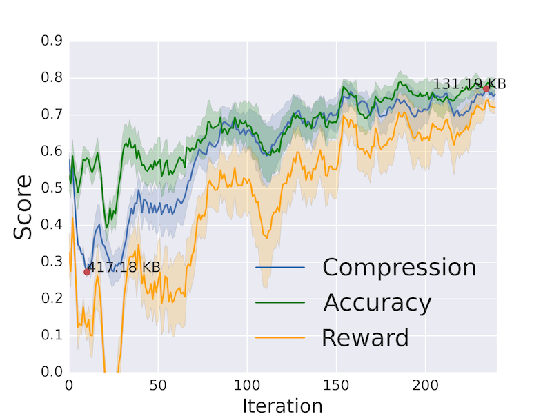
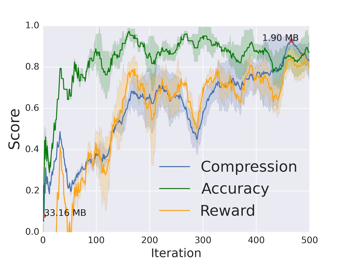
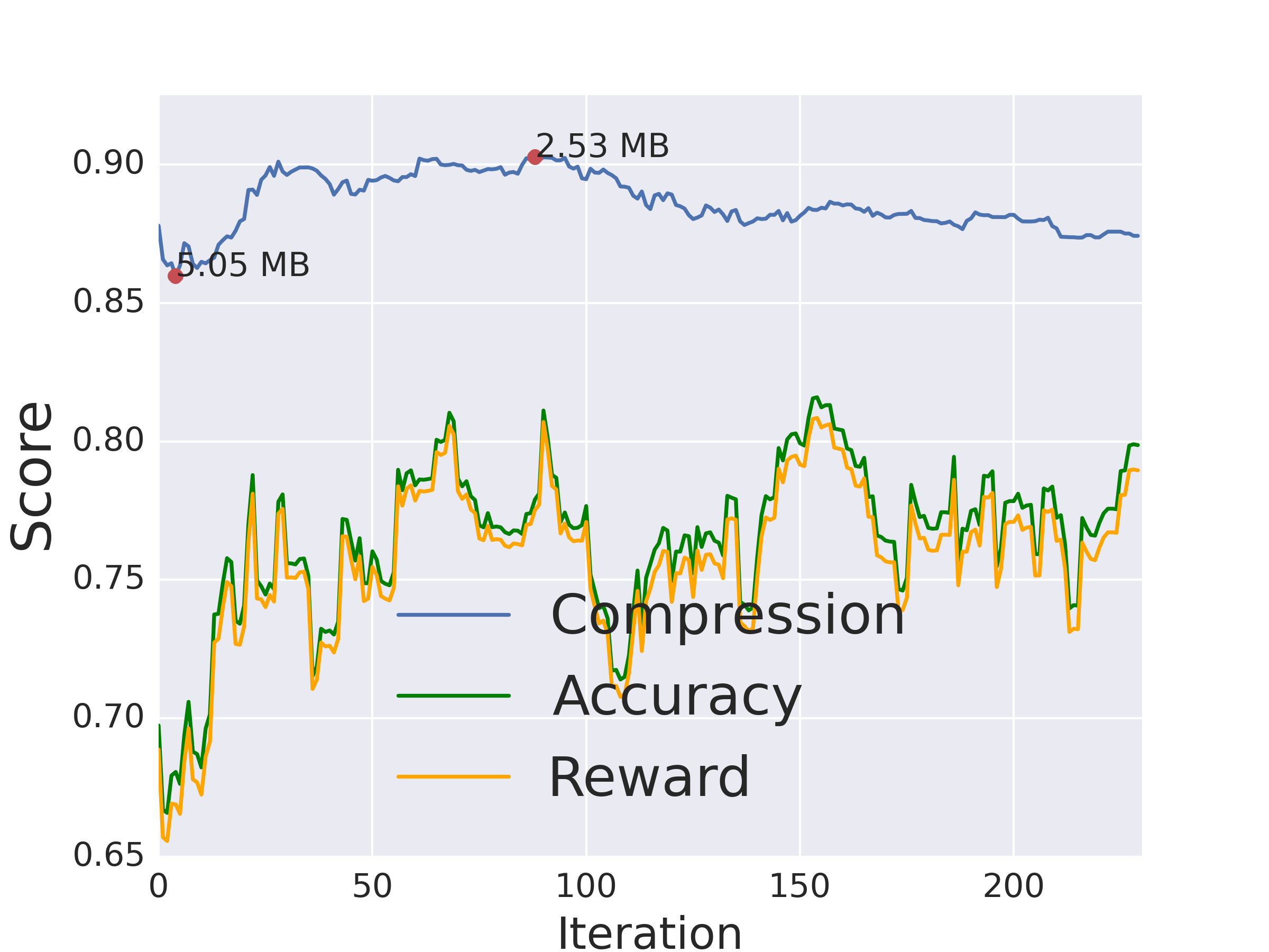
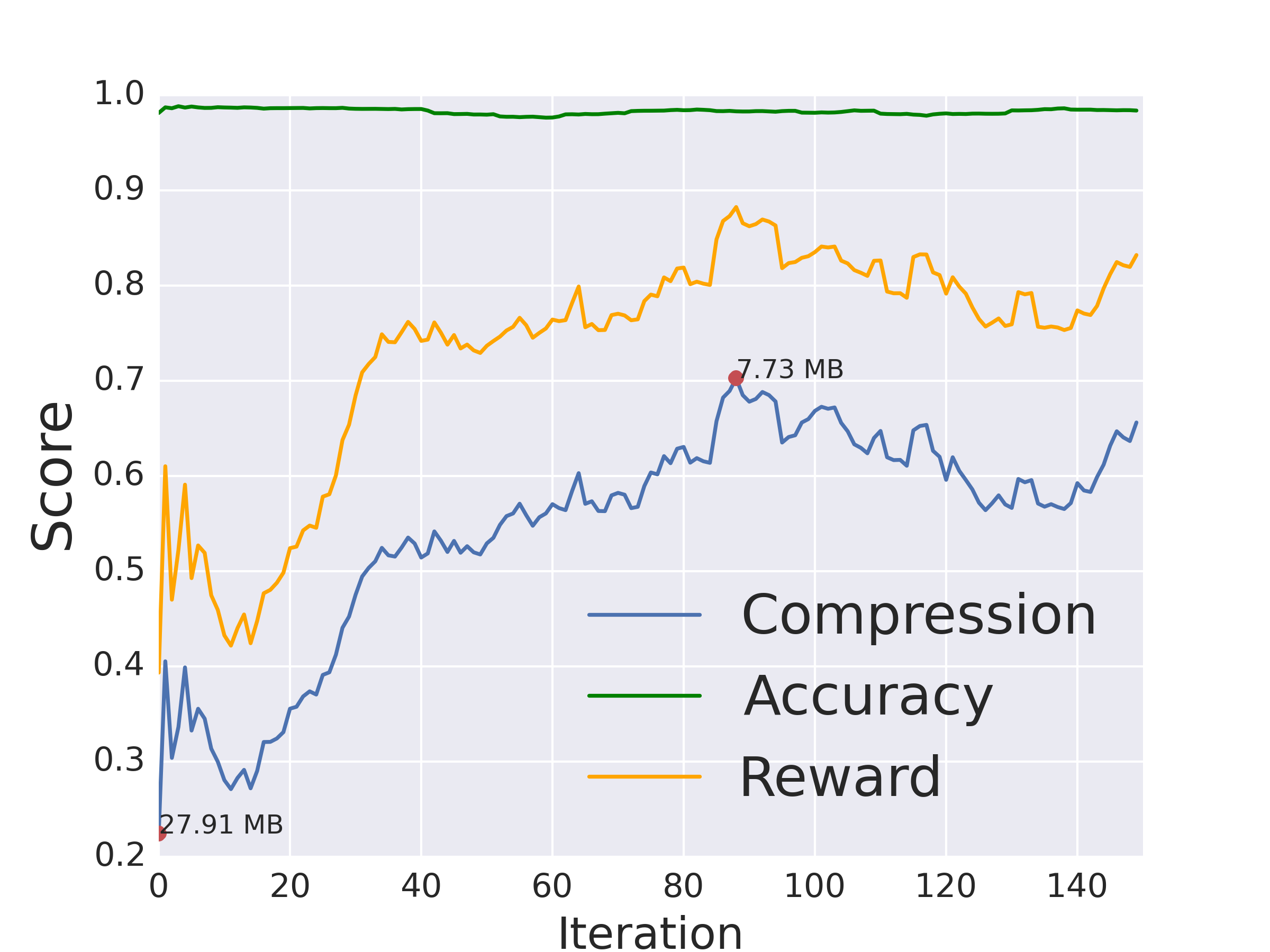
MNIST To evaluate the compression performance we use (1) a Conv4 network consisting of 4 convolutional layers and (2) a high capacity VGG-13 network.
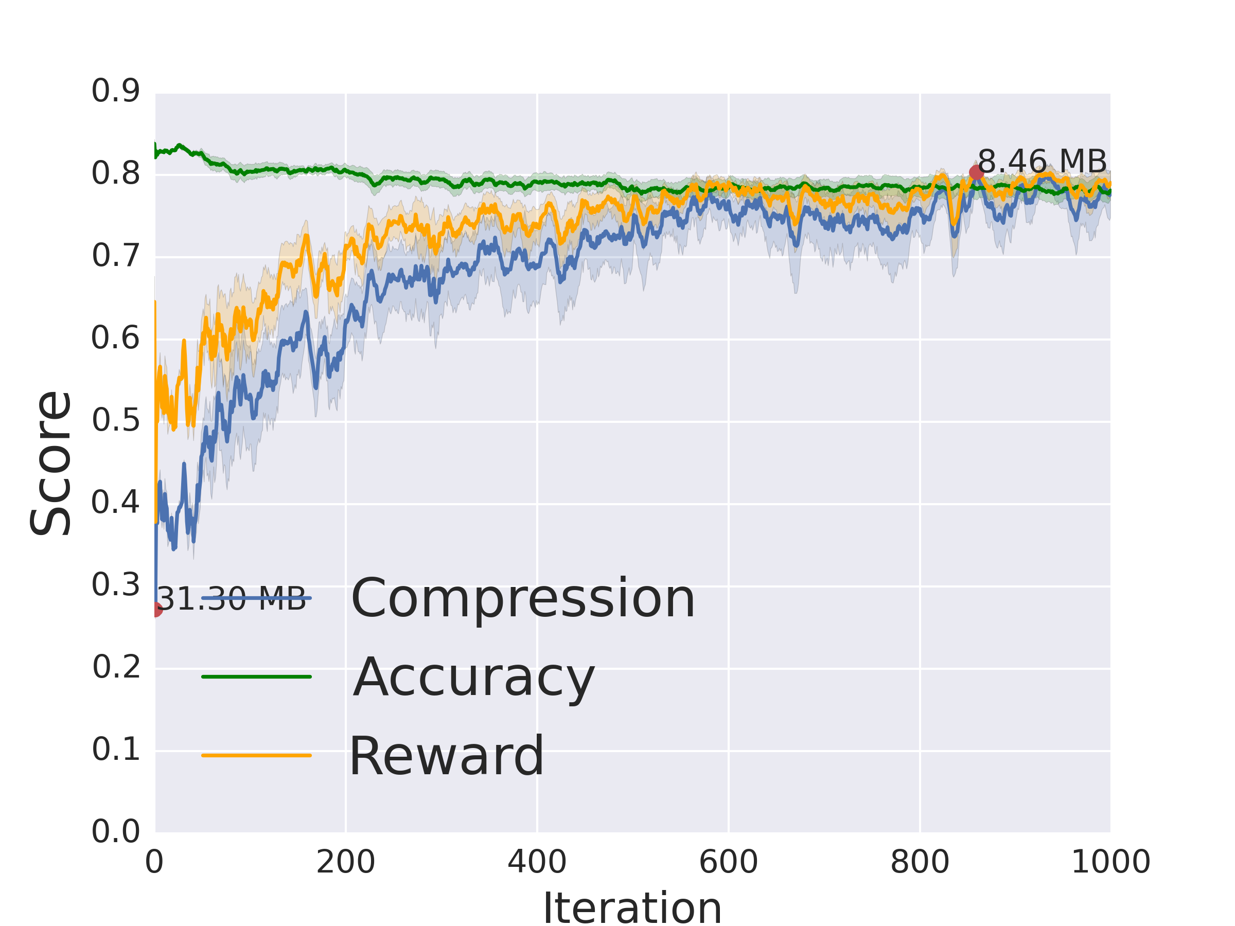
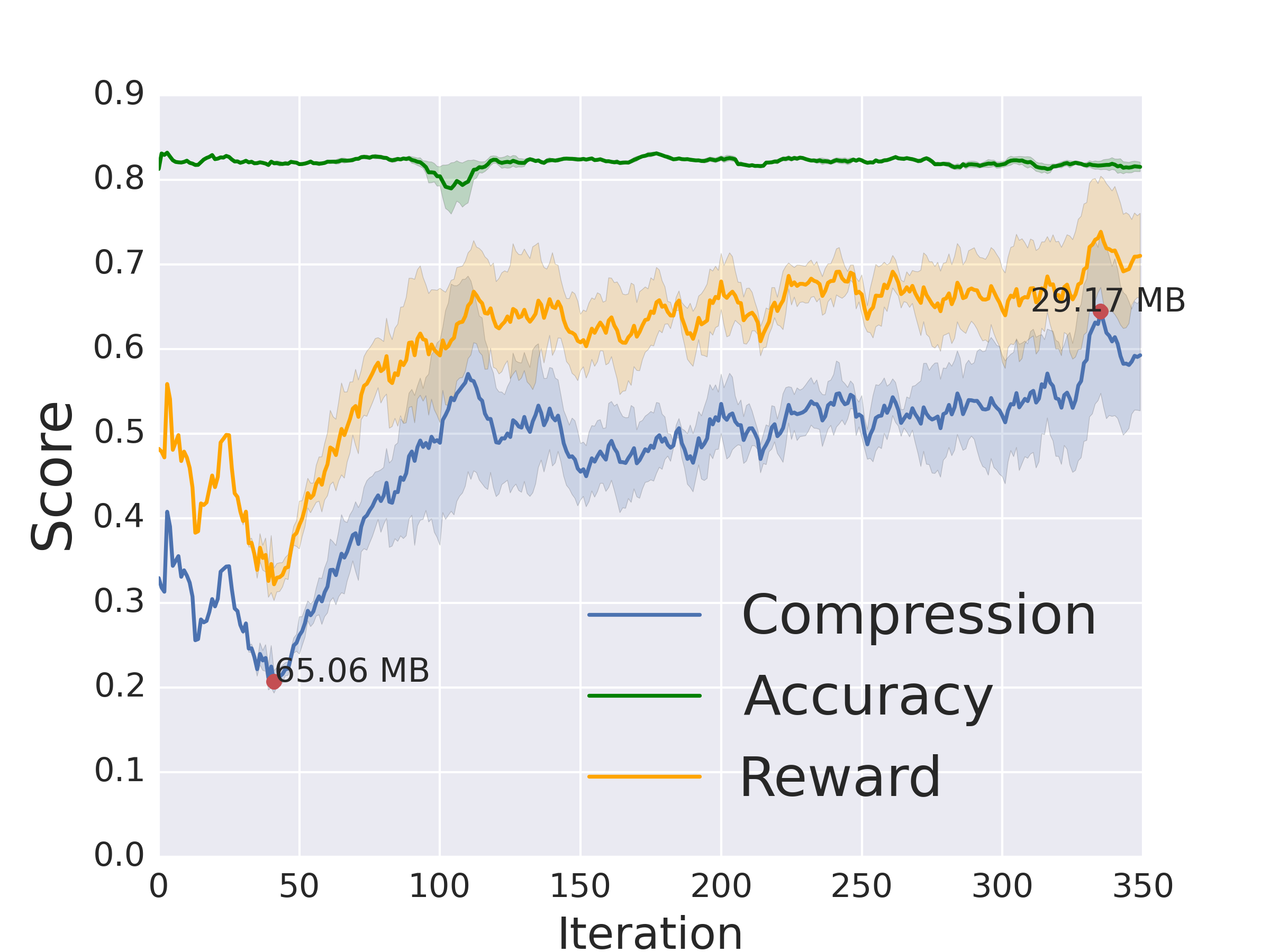
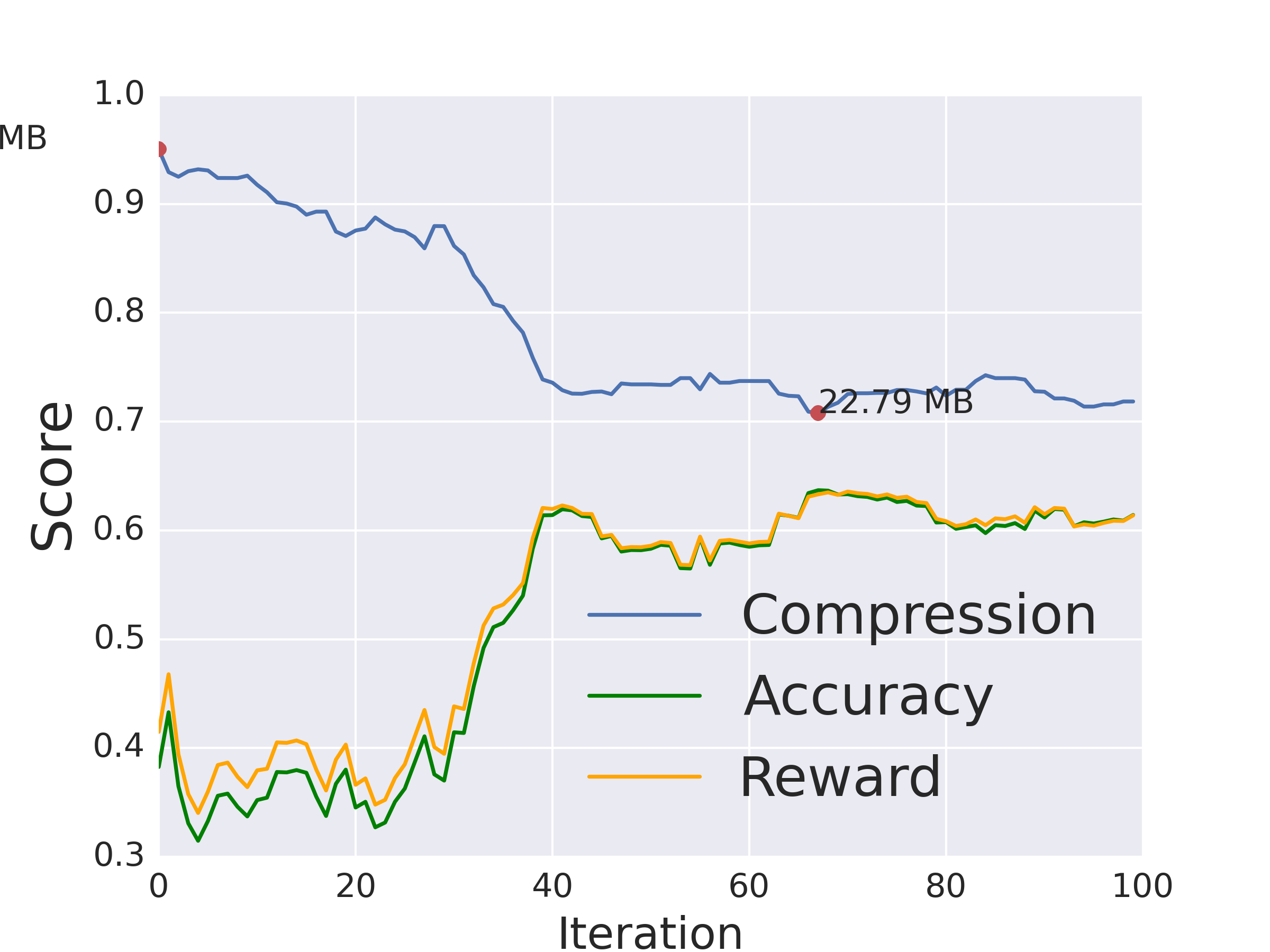
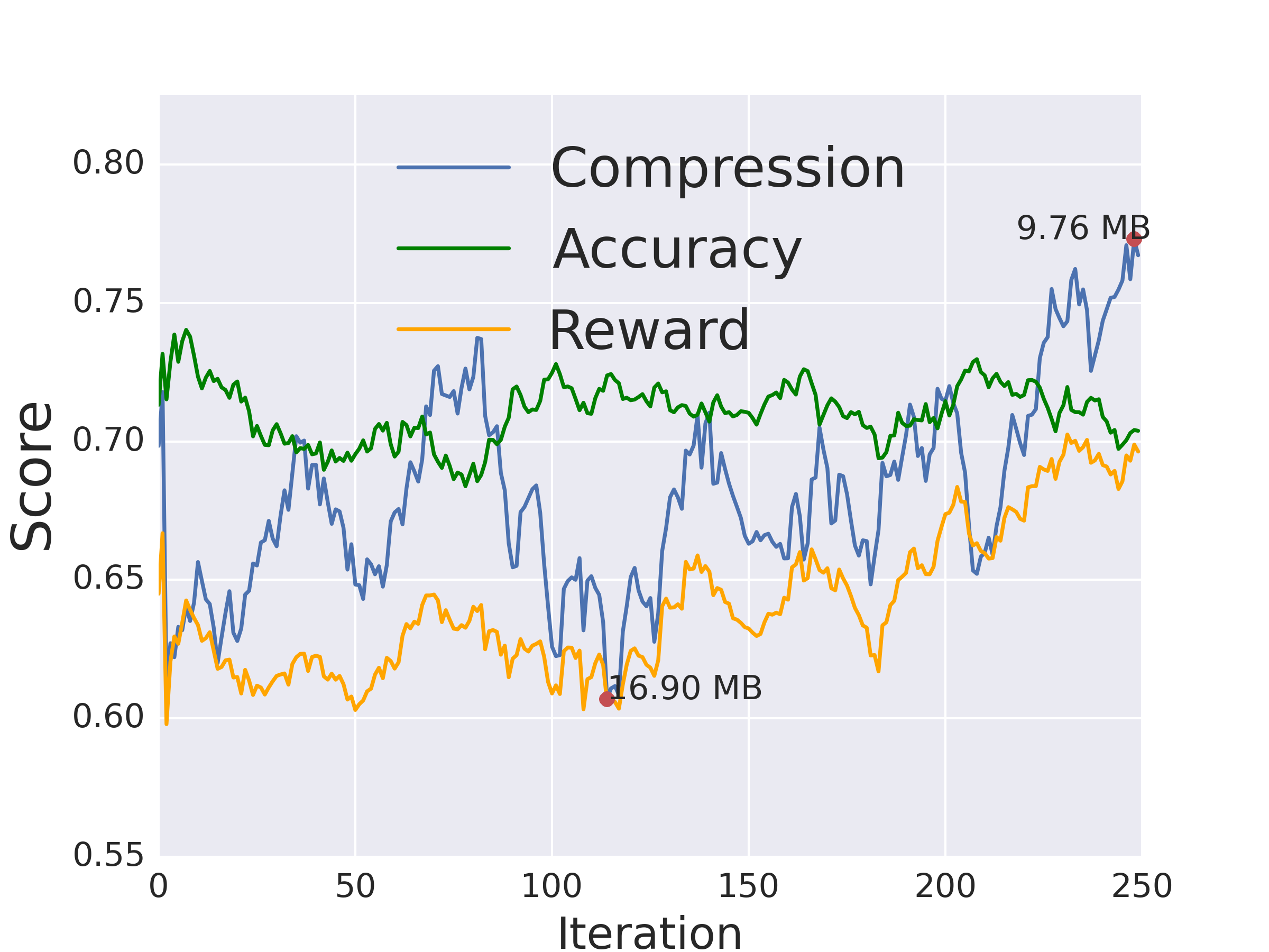
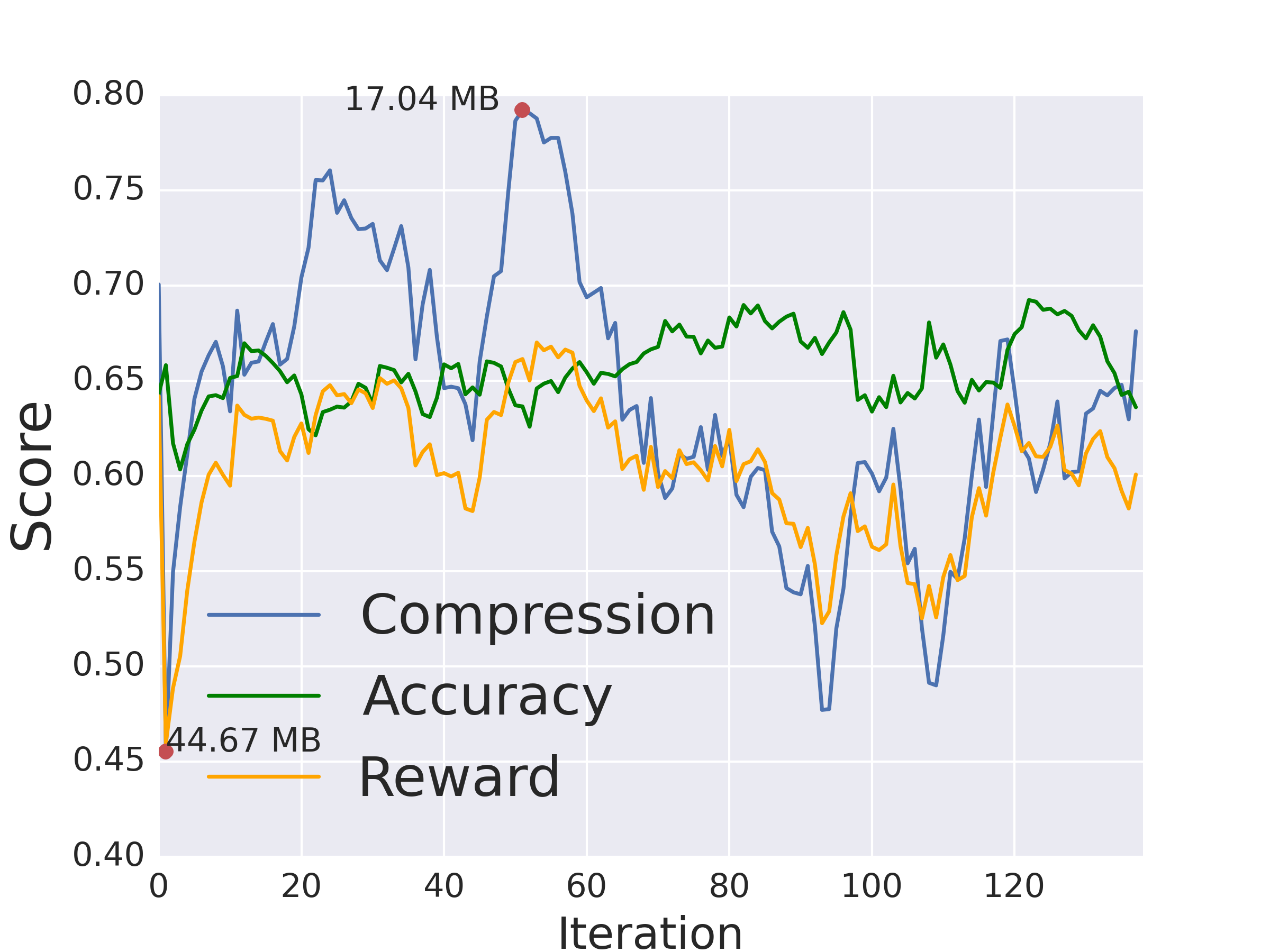
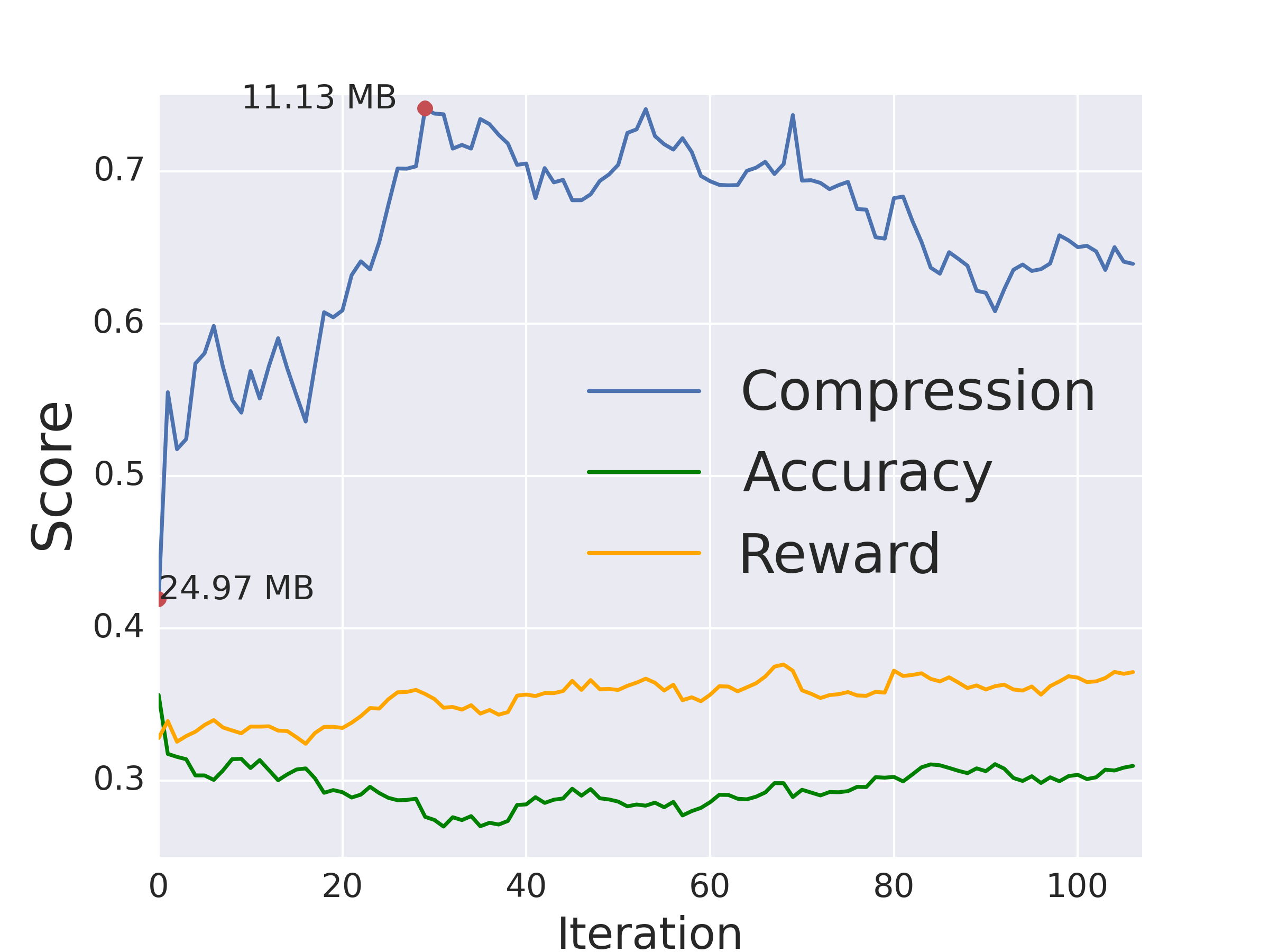
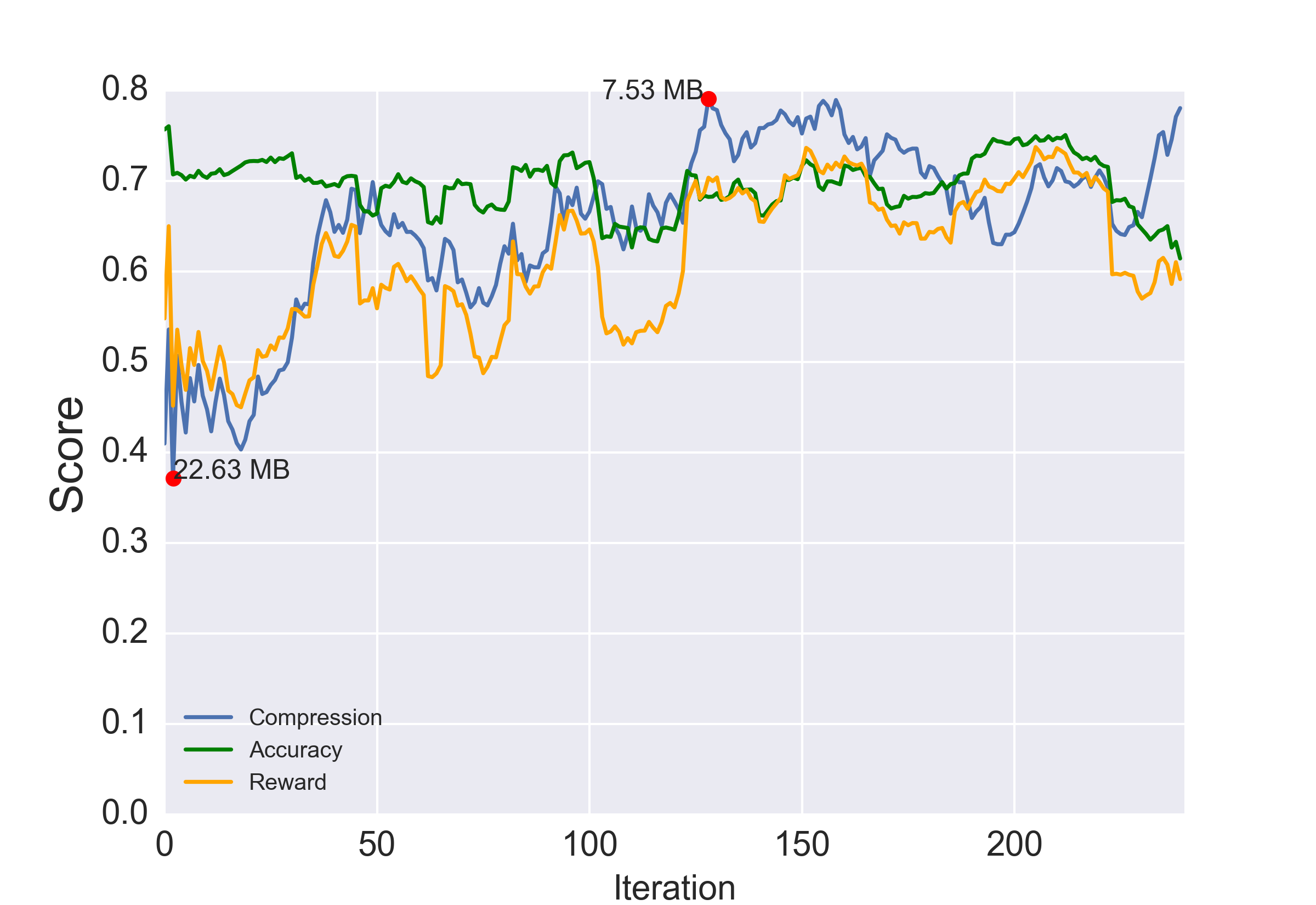
Figure 3 shows the results of our compression approach for each teacher network. The lines represent the compression (blue), accuracy (green) and reward (orange). The y-axis represents the score of those quantities, between 0 and 1. The x-axis is the iteration number. We also highlight the largest and smallest models with red circles to give a sense of the magnitude of compression. This experiment appears to confirm our original expectation that the policies would improve over time.
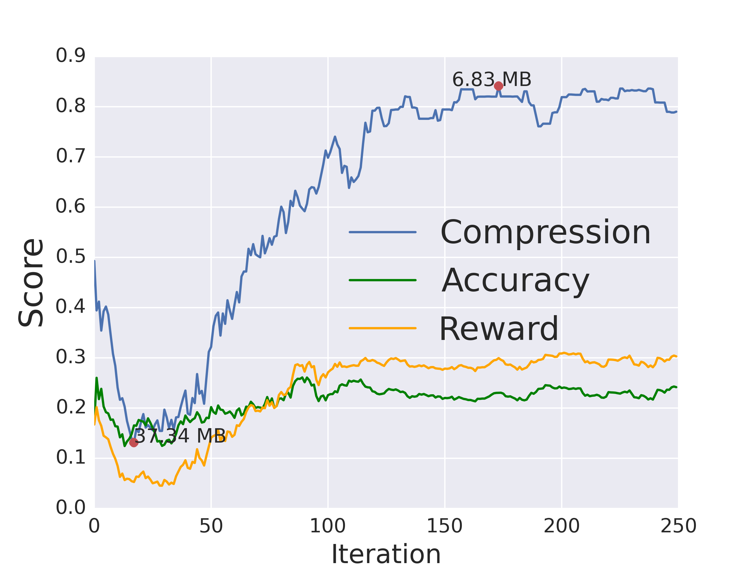
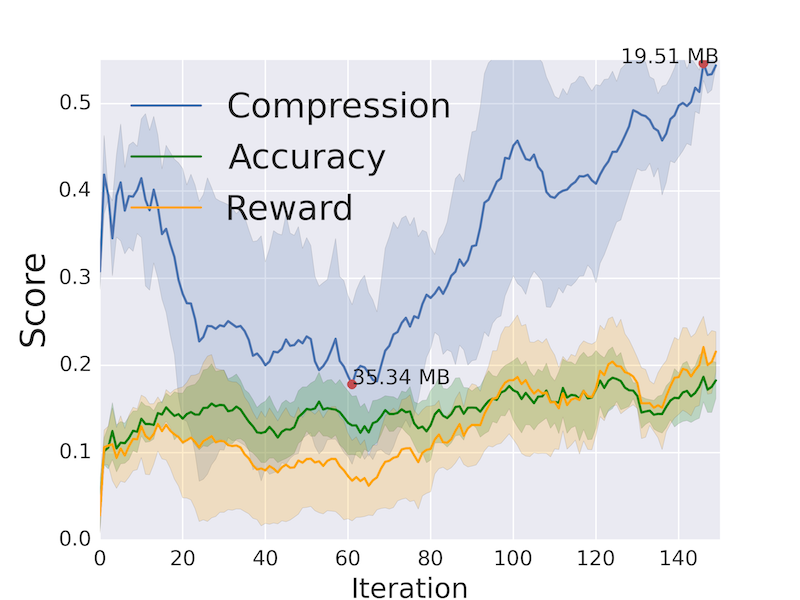
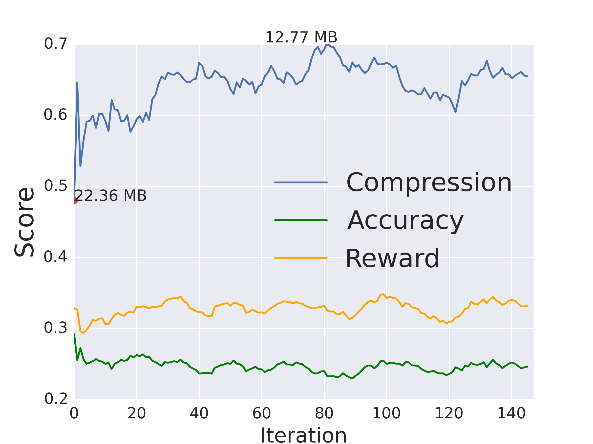
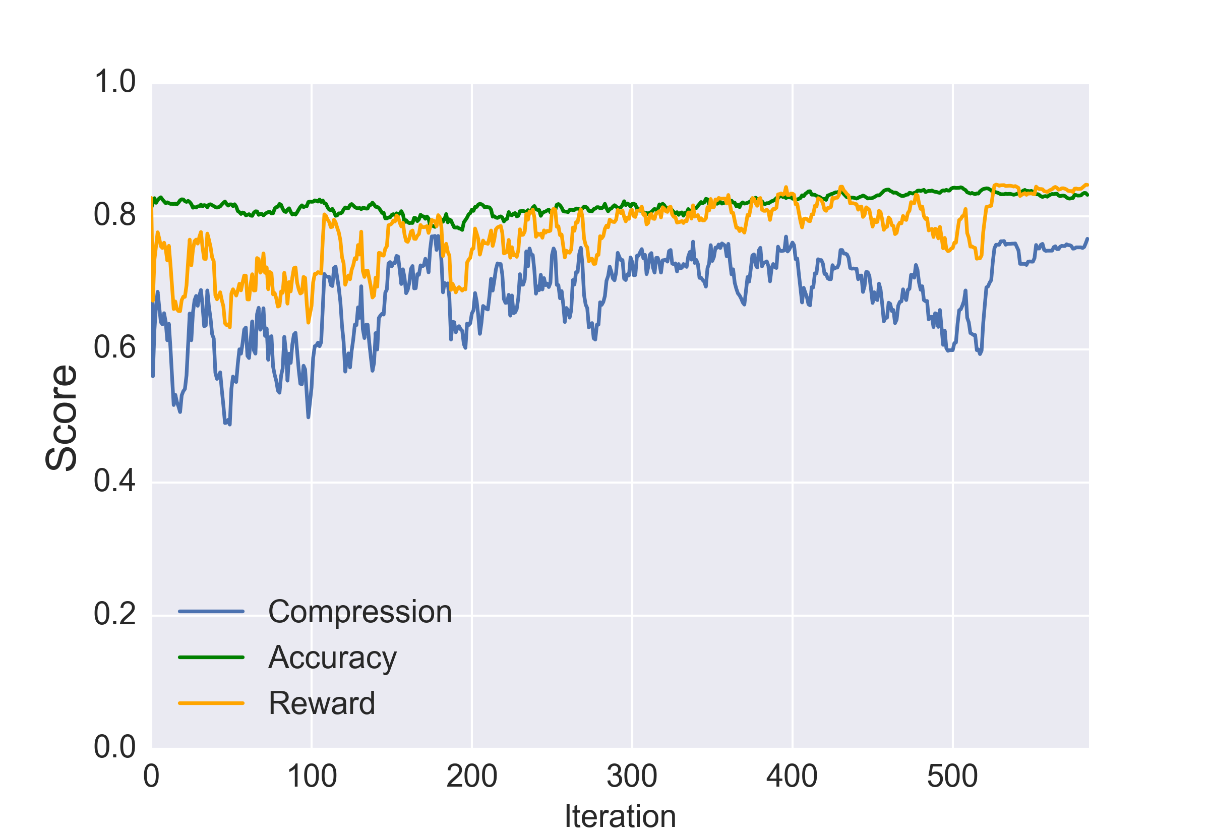
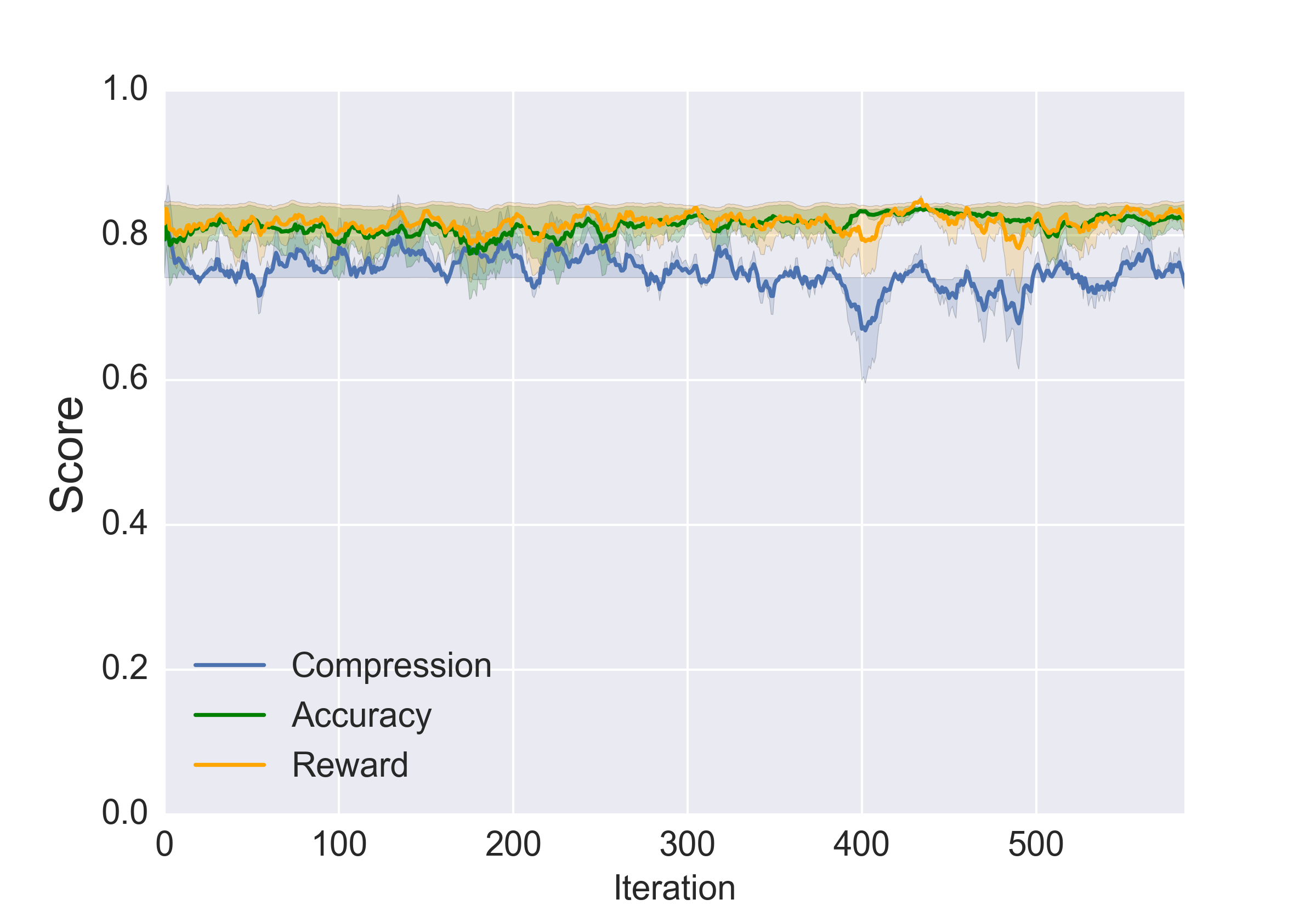
CIFAR-10 On the CIFAR-10 dataset we ran experiments using the following teacher networks: (1) VGG-19, (2) ResNet-18 and (3) ResNet-34 networks. The experimental results are shown in Figure 4. It is interesting to note that on CIFAR-10, our learned student networks perform almost as well or better the teacher networks despite a 10x compression rate.
SVHN On the SVHN dataset, we ran experiments using ResNet-18 network as the teacher model. We observed that the reward and compression steadily increased while the accuracy remained stable, confirming similar results to that of CIFAR-10. This is a promising indication that our approach works for a breadth of tasks and isn’t dataset specific. Results are in the appendix.
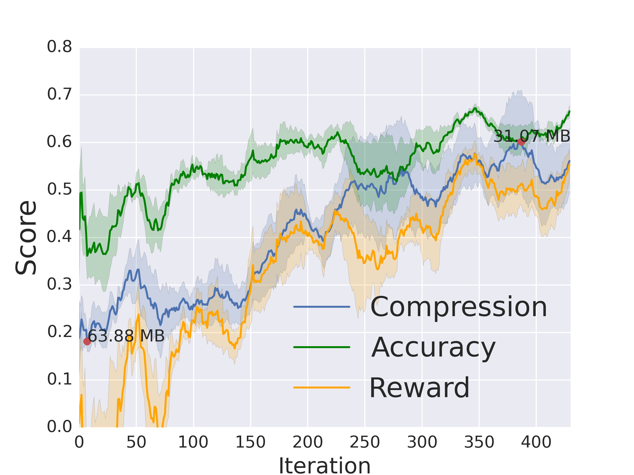
CIFAR-100 We also verified our approach on a harder dataset, CIFAR-100 to show how our approach performs with less data per class (Figure 5). Considering the largely reduced number of parameters, the compressed network achieves reasonably high accuracy. A notable aspect of many of the final compressed models is that ReLU layers within residual blocks were removed. Another interesting result is that the compressed ResNet-34 student model outperforms the ResNet-18 model despite having fewer parameters. This can likely be explained by the increased number of residual blocks in the ResNet-34 model.
Caltech-256 The Caltech-256 experiments (appendix) show the performance of our approach when training data is scarce. We would like to verify that our approach does not overly compress the network by overfitting to the small number of training examples. As with the other experiments, the policies appears to learn to maximize reward over time, although the positive trend is not as pronounced due to the lack of training data. This is expected since less data means the reward signal is less robust to sources of noise, which in turn affects training of the policy.
4.4 Baselines
We compare the performance of our approach to current model compression methods, namely pruning and Knowledge Distillation (with hand-designed model). We note here that compression rate is defined as the ratio of number of parameters instead of number of bits, which some other compression methods (quantization, coding) use. To provide a fair comparison with our method, the same trained teacher models used in our method were used.
4.4.1 Pruning
| Model | Acc. | #Params | Compr. | Acc. |
|---|---|---|---|---|
| Teacher (MNIST/VGG-13) | 99.54% | 9.4M | — | — |
| Pruning | 99.12% | 162K | 58x | -0.42% |
| Ours | 99.55% | 73K | 127x | +0.01% |
| Teacher (CIFAR-10/VGG-19) | 91.97% | 20.2M | — | — |
| Pruning | 91.06% | 2.3M | 8.7x | -0.91% |
| Ours | 92.05% | 1.7M | 11.8x | +0.08% |
We compare our method to pruning, which is a model compression approach that operates directly on the weight space of a network, removing redundant weights or filters. We perform pruning based on Molchanov et al. (2016), which removes filters using a greedy criteria based approach and then finetunes the network. With pruning, the performance of the final model can vary depending on the degree to which it was pruned. To ensure a fair comparison, we stop pruning when 1. accuracy drops below 1% of the student model obtained by our method or 2. the number of parameters is less than our method. Pruning is done 5 times to control for variance and the best performing model is reported.
The results of this experiment, reported in Table 2, show that while the pruned models show good compression rates, our approach outperforms this baseline on both datasets. These results could indicate that operating on the architecture space of the model might result in more consistent results than using heuristics to operate on the weight space directly.
4.4.2 Knowledge Distillation
| Model | Acc. | #Params | Compr. | Acc. |
| Teacher (SVHN/ResNet-18) | 95.24% | 11.17M | — | — |
| SqueezeNet1.1 | 89.34% | 727K | 15x | -5.90% |
| Ours | 95.38% | 564K | 19.8x | +0.18% |
| Teacher (CIFAR-10/ResNet-18) | 92.01% | 11.17M | — | — |
| FitNet-4 | 91.33% | 1.2M | 9.3x | -0.63% |
| VGG-small | 83.93% | 1.06M | 10.5x | -8.08% |
| Ours | 91.81% | 1.00M | 11.0x | -0.20% |
We also tested the validity of our hypothesis that hand designed models may not be optimal for Knowledge distillation. We compare models generated by our method to hand designed models that contain a similar number of parameters. We perform experiments with 3 hand designed model architectures, FitNet-4, SqueezeNet and a reduced network based on VGG, (VGG-small) which contains 10 layers. These networks were then trained to convergence with Knowledge Distillation on the CIFAR-10 dataset and the SVHN datasets.
For the implementation of FitNet-4 (17 layers), we used the same model architecture described in Mishkin & Matas (2015) with the ReLU activation and Xavier initialization. The paper reported a baseline accuracy of 90.63 when trained from scratch and 1.2 M parameters (Table 3 in Mishkin & Matas (2015)). For SqueezeNet, we implemented the 1.1 version described in Iandola et al. (2016), which contained 727K parameters after adapting it to CIFAR-10. We benchmarked VGG-small and FitNet on the CIFAR-10 dataset and SqueezeNet on the SVHN dataset in order to provide a fair comparison with our best models in terms of the number of parameters.
From the results reported in Table 3, we observe that our method performs better than the hand-designed models on both datasets despite containing fewer parameters. The CIFAR-10 results seem to indicate that model selection is an important factor in Knowledge Distillation. Our model and the FitNet-4 model both outperform the VGG-small model, further confirming our hypothesis that hand-designing models may not be the optimal approach for use with Knowledge Distillation.
4.5 Compression with Size Constraints
| Model | Acc. | #Params | Compr. | Constr. |
|---|---|---|---|---|
| Teacher (MNIST/VGG-13) | 99.54% | 9.4M | 1x | N/A |
| Student (Stage 1 & 2) | 98.91% | 17K | 553x | 20K |
| Teacher (CIFAR-10/VGG-19) | 91.97% | 20.2M | 1x | N/A |
| Student (Stage 1 & 2) | 90.8% | 573K | 35x | 1M |
While the experiments to this point used no explicit constraints, in this experiment, we add a size constraint in terms of the number of parameters via the reward function as in Section 3.3.1. We expect the optimization to be harder because the range of acceptable architectures is reduced.
Results are summarized in Table 4. These promising results suggest that the compression policies are able to produce sensible results despite being heavily constrained, thus demonstrating the viability of the approach in practice.
4.6 Transfer Learning
| ResNet18 ResNet34 | ResNet34 ResNet18 | VGG11 VGG19 | |||||||||
|---|---|---|---|---|---|---|---|---|---|---|---|
| Reward | Comp. | Acc. | Reward | Comp. | Acc. | Reward | Comp. | Acc. | |||
| Pre-trained | 0.81 | 78.1% | 79.5% | 0.76 | 65.5% | 82.3% | 0.52 | 46.0% | 71.7% | ||
| Scratch | 0.50 | 34.8% | 82.4% | 0.53 | 39.7% | 82.8% | -0.07 | 20.2% | 42.5 % | ||
Naively applying our approach to a new teacher network means that the compression policies must be learned from scratch for each new problem. We would like to know if layer removal and shrinkage policy networks can be reused to accelerate compression for new teacher architectures. In the following experiments, we train a policy on an initial teacher model and then apply it to another teacher model to test whether the policy has learned a general strategy for compressing a network. Since both a pretrained policy and a randomly initialized policy is expected to eventually converge to a locally optimal policy given enough iterations, we provide performance measures over the the first 10 policy update iterations.
Results are summarized in Table 5. The slight drop in accuracy (third subcolumn) in models produced by the pretrained policy is expected due to the tradeoff between compression and accuracy. However, the average reward (first subcolumn) is always higher when we use a pretrained policy. Note that in the VGG experiment, the reward is negative since the non-pretrained policy starts off by producing degenerate models. However, the pretrained policy starts off from a different initialization that does not.
This is an important result as it shows promising evidence that we can even transfer learned knowledge from a smaller model to a larger model, rapidly accelerating the policy search procedure on very deep networks.
5 Conclusion
We introduced a novel method for compressing neural networks. Our approach employs a two-stage layer removal and layer shrinkage procedure to learn how to compress large neural networks. By leveraging signals for accuracy and compression as supervision, our method efficiently learns to search the space of model architectures. We show that our method performs well over a variety of datasets and architectures. We also observe generalization capabilities of our method through transfer learning, allowing our procedure to be made even more efficient. Our method is also able to incorporate other practical constraints, such as power or inference time, thus showing potential for application in a real world setting.
References
- Anwar et al. (2015) Sajid Anwar, Kyuyeon Hwang, and Wonyong Sung. Structured pruning of deep convolutional neural networks. arXiv preprint arXiv:1512.08571, 2015.
- Ba & Caruana (2014) Jimmy Ba and Rich Caruana. Do deep nets really need to be deep? In Advances in neural information processing systems, pp. 2654–2662, 2014.
- Baker et al. (2016) Bowen Baker, Otkrist Gupta, Nikhil Naik, and Ramesh Raskar. Designing neural network architectures using reinforcement learning. arXiv preprint arXiv:1611.02167, 2016.
- Buciluǎ et al. (2006) Cristian Buciluǎ, Rich Caruana, and Alexandru Niculescu-Mizil. Model compression. In Proceedings of the 12th ACM SIGKDD international conference on Knowledge discovery and data mining, pp. 535–541. ACM, 2006.
- Cox & Pinto (2011) David Cox and Nicolas Pinto. Beyond simple features: A large-scale feature search approach to unconstrained face recognition. In Automatic Face & Gesture Recognition and Workshops (FG 2011), 2011 IEEE International Conference on, pp. 8–15. IEEE, 2011.
- Feng & Darrell (2015) Jiashi Feng and Trevor Darrell. Learning the structure of deep convolutional networks. In Proceedings of the IEEE International Conference on Computer Vision, pp. 2749–2757, 2015.
- Griffin et al. (2007) Gregory Griffin, Alex Holub, and Pietro Perona. Caltech-256 object category dataset. 2007.
- Guo et al. (2016) Yiwen Guo, Anbang Yao, and Yurong Chen. Dynamic network surgery for efficient dnns. In Advances In Neural Information Processing Systems, pp. 1379–1387, 2016.
- Han et al. (2015a) Song Han, Huizi Mao, and William J Dally. Deep compression: Compressing deep neural networks with pruning, trained quantization and huffman coding. arXiv preprint arXiv:1510.00149, 2015a.
- Han et al. (2015b) Song Han, Jeff Pool, John Tran, and William Dally. Learning both weights and connections for efficient neural network. In Advances in Neural Information Processing Systems, pp. 1135–1143, 2015b.
- Hassibi et al. (1993) Babak Hassibi, David G Stork, and Gregory J Wolff. Optimal brain surgeon and general network pruning. In Neural Networks, 1993., IEEE International Conference on, pp. 293–299. IEEE, 1993.
- Hinton et al. (2015) Geoffrey Hinton, Oriol Vinyals, and Jeff Dean. Distilling the knowledge in a neural network. arXiv preprint arXiv:1503.02531, 2015.
- Iandola et al. (2016) Forrest N Iandola, Song Han, Matthew W Moskewicz, Khalid Ashraf, William J Dally, and Kurt Keutzer. Squeezenet: Alexnet-level accuracy with 50x fewer parameters and¡ 0.5 mb model size. arXiv preprint arXiv:1602.07360, 2016.
- Jarrett et al. (2009) Kevin Jarrett, Koray Kavukcuoglu, Yann LeCun, et al. What is the best multi-stage architecture for object recognition? In Computer Vision, 2009 IEEE 12th International Conference on, pp. 2146–2153. IEEE, 2009.
- Jozefowicz et al. (2015) Rafal Jozefowicz, Wojciech Zaremba, and Ilya Sutskever. An empirical exploration of recurrent network architectures. In Proceedings of the 32nd International Conference on Machine Learning (ICML-15), pp. 2342–2350, 2015.
- Krizhevsky & Hinton (2009) Alex Krizhevsky and Geoffrey Hinton. Learning multiple layers of features from tiny images. 2009.
- LeCun et al. (1989) Yann LeCun, John S Denker, Sara A Solla, Richard E Howard, and Lawrence D Jackel. Optimal brain damage. In NIPs, volume 2, pp. 598–605, 1989.
- LeCun et al. (1998) Yann LeCun, Corinna Cortes, and Christopher JC Burges. The mnist database of handwritten digits, 1998.
- Ludermir et al. (2006) Teresa B Ludermir, Akio Yamazaki, and Cleber Zanchettin. An optimization methodology for neural network weights and architectures. IEEE Transactions on Neural Networks, 17(6):1452–1459, 2006.
- Mariet & Sra (2015) Zelda Mariet and Suvrit Sra. Diversity networks. arXiv preprint arXiv:1511.05077, 2015.
- Miikkulainen et al. (2017) Risto Miikkulainen, Jason Liang, Elliot Meyerson, Aditya Rawal, Dan Fink, Olivier Francon, Bala Raju, Arshak Navruzyan, Nigel Duffy, and Babak Hodjat. Evolving deep neural networks. arXiv preprint arXiv:1703.00548, 2017.
- Mishkin & Matas (2015) Dmytro Mishkin and Jiri Matas. All you need is a good init. arXiv preprint arXiv:1511.06422, 2015.
- Molchanov et al. (2016) Pavlo Molchanov, Stephen Tyree, Tero Karras, Timo Aila, and Jan Kautz. Pruning convolutional neural networks for resource efficient inference. 2016.
- Murdock et al. (2016) Calvin Murdock, Zhen Li, Howard Zhou, and Tom Duerig. Blockout: Dynamic model selection for hierarchical deep networks. In Proceedings of the IEEE Conference on Computer Vision and Pattern Recognition, pp. 2583–2591, 2016.
- Netzer et al. (2011) Yuval Netzer, Tao Wang, Adam Coates, Alessandro Bissacco, Bo Wu, and Andrew Y Ng. Reading digits in natural images with unsupervised feature learning. In NIPS workshop on deep learning and unsupervised feature learning, volume 2011, pp. 5, 2011.
- Real et al. (2017) Esteban Real, Sherry Moore, Andrew Selle, Saurabh Saxena, Yutaka Leon Suematsu, Quoc Le, and Alex Kurakin. Large-scale evolution of image classifiers. arXiv preprint arXiv:1703.01041, 2017.
- Romero et al. (2014) Adriana Romero, Nicolas Ballas, Samira Ebrahimi Kahou, Antoine Chassang, Carlo Gatta, and Yoshua Bengio. Fitnets: Hints for thin deep nets. arXiv preprint arXiv:1412.6550, 2014.
- Saxe et al. (2011) Andrew Saxe, Pang W Koh, Zhenghao Chen, Maneesh Bhand, Bipin Suresh, and Andrew Y Ng. On random weights and unsupervised feature learning. In Proceedings of the 28th international conference on machine learning (ICML-11), pp. 1089–1096, 2011.
- Simonyan & Zisserman (2014) Karen Simonyan and Andrew Zisserman. Very deep convolutional networks for large-scale image recognition. arXiv preprint arXiv:1409.1556, 2014.
- Snoek et al. (2012) Jasper Snoek, Hugo Larochelle, and Ryan P Adams. Practical bayesian optimization of machine learning algorithms. In Advances in neural information processing systems, pp. 2951–2959, 2012.
- Snoek et al. (2015) Jasper Snoek, Oren Rippel, Kevin Swersky, Ryan Kiros, Nadathur Satish, Narayanan Sundaram, Mostofa Patwary, Mr Prabhat, and Ryan Adams. Scalable bayesian optimization using deep neural networks. In International Conference on Machine Learning, pp. 2171–2180, 2015.
- Srinivas & Babu (2015) Suraj Srinivas and R Venkatesh Babu. Data-free parameter pruning for deep neural networks. arXiv preprint arXiv:1507.06149, 2015.
- Stanley & Miikkulainen (2002) Kenneth O Stanley and Risto Miikkulainen. Evolving neural networks through augmenting topologies. Evolutionary computation, 10(2):99–127, 2002.
- Urban et al. (2016) Gregor Urban, Krzysztof J Geras, Samira Ebrahimi Kahou, Ozlem Aslan, Shengjie Wang, Rich Caruana, Abdelrahman Mohamed, Matthai Philipose, and Matt Richardson. Do deep convolutional nets really need to be deep and convolutional? arXiv preprint arXiv:1603.05691, 2016.
- Warde-Farley et al. (2014) David Warde-Farley, Andrew Rabinovich, and Dragomir Anguelov. Self-informed neural network structure learning. arXiv preprint arXiv:1412.6563, 2014.
- Wierstra et al. (2010) Daan Wierstra, Alexander Förster, Jan Peters, and Jürgen Schmidhuber. Recurrent policy gradients. Logic Journal of IGPL, 18(5):620–634, 2010.
- Williams (1992) Ronald J Williams. Simple statistical gradient-following algorithms for connectionist reinforcement learning. Machine learning, 8(3-4):229–256, 1992.
- Zoph & Le (2016) Barret Zoph and Quoc V Le. Neural architecture search with reinforcement learning. arXiv preprint arXiv:1611.01578, 2016.
Appendix
6 Actor-Critic
Policy gradient based Actor-Critic algorithms have been shown to improve the stability of the policy search. This is achieved by replacing the baseline with a learned estimate of the value function at each time step.
Formally, with vanilla REINFORCE we have,
In the Actor-Critic algorithm we replace with , resulting in a new gradient estimate,
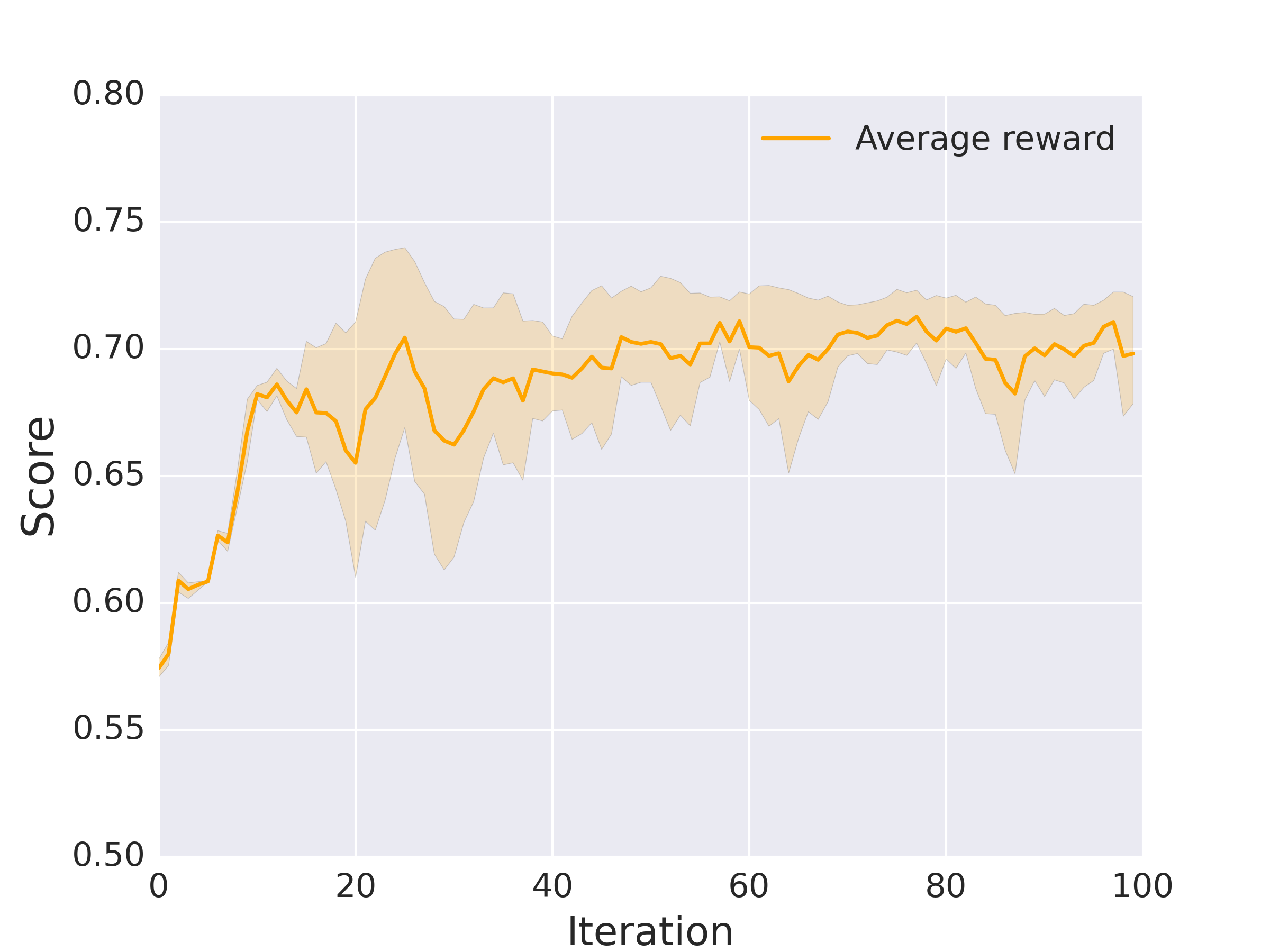
We implement the Critic network by adding an additional fully-connected layer that takes as input the hidden state of the LSTM and outputs a single scalar value. Below are the results of the experiments performed.
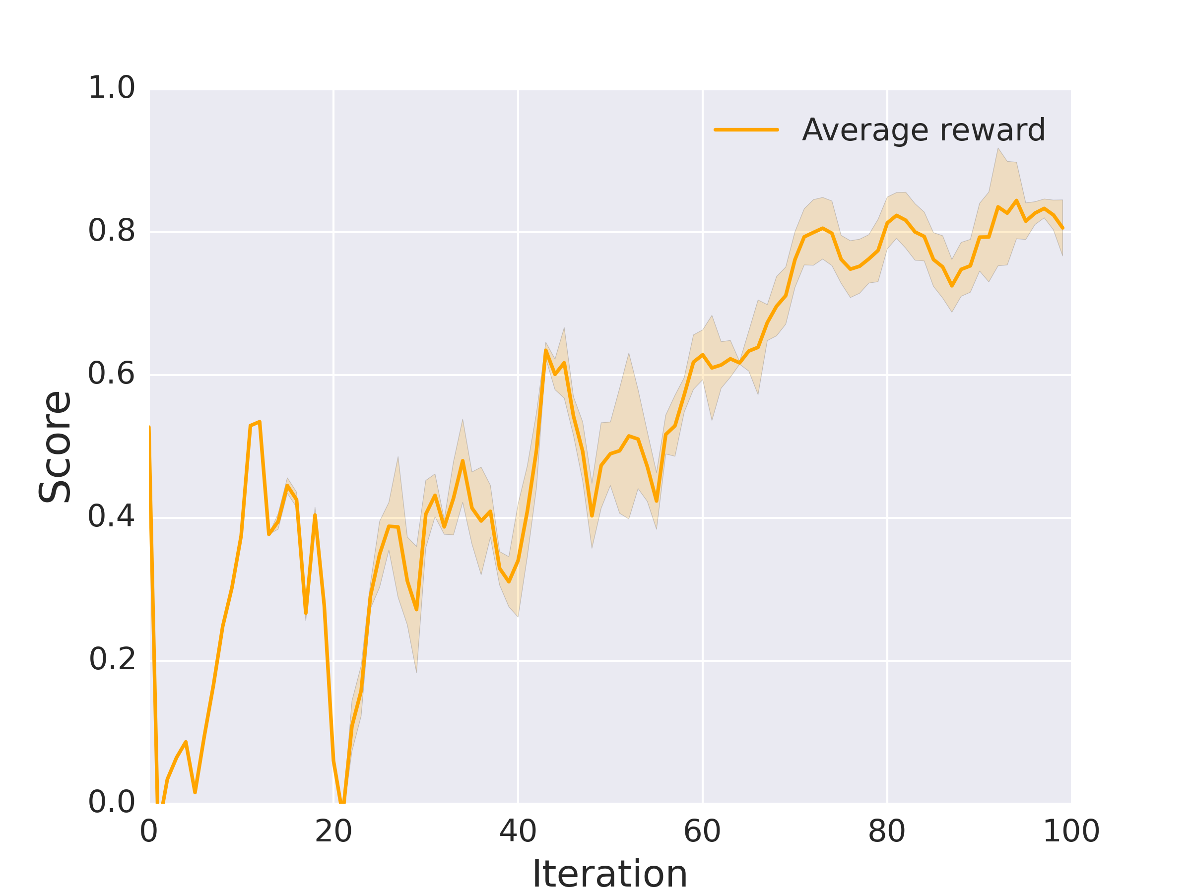
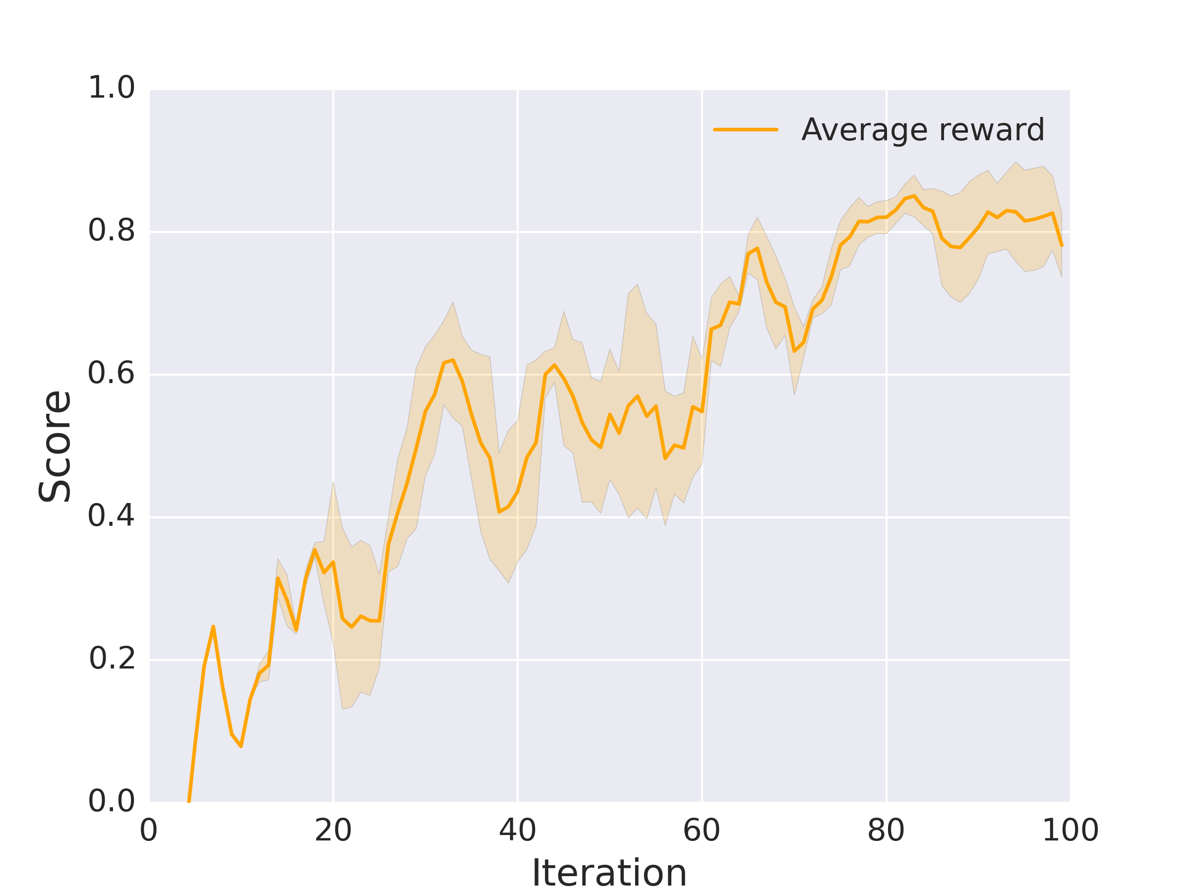
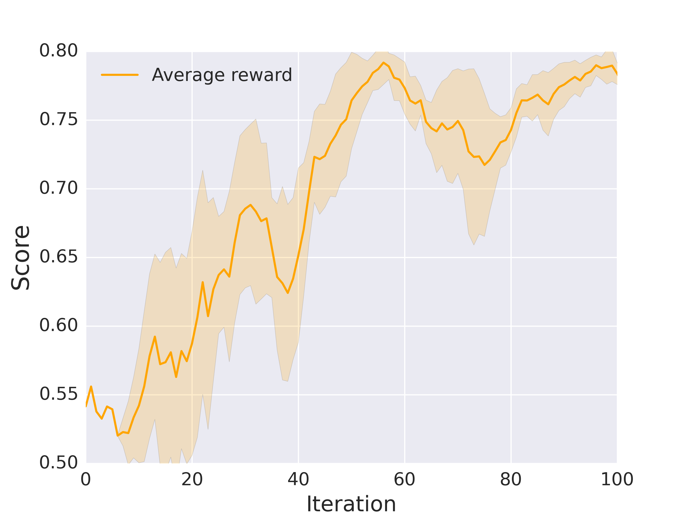
For the MNIST dataset, our results show that there is a slight improvement in stability, although they both converge at a similar rate.
For the CIFAR-10 dataset, although the Actor-critic version was more stable, it did not perform as well as the vanilla REINFORCE algorithm.
7 Learning rate and batch size
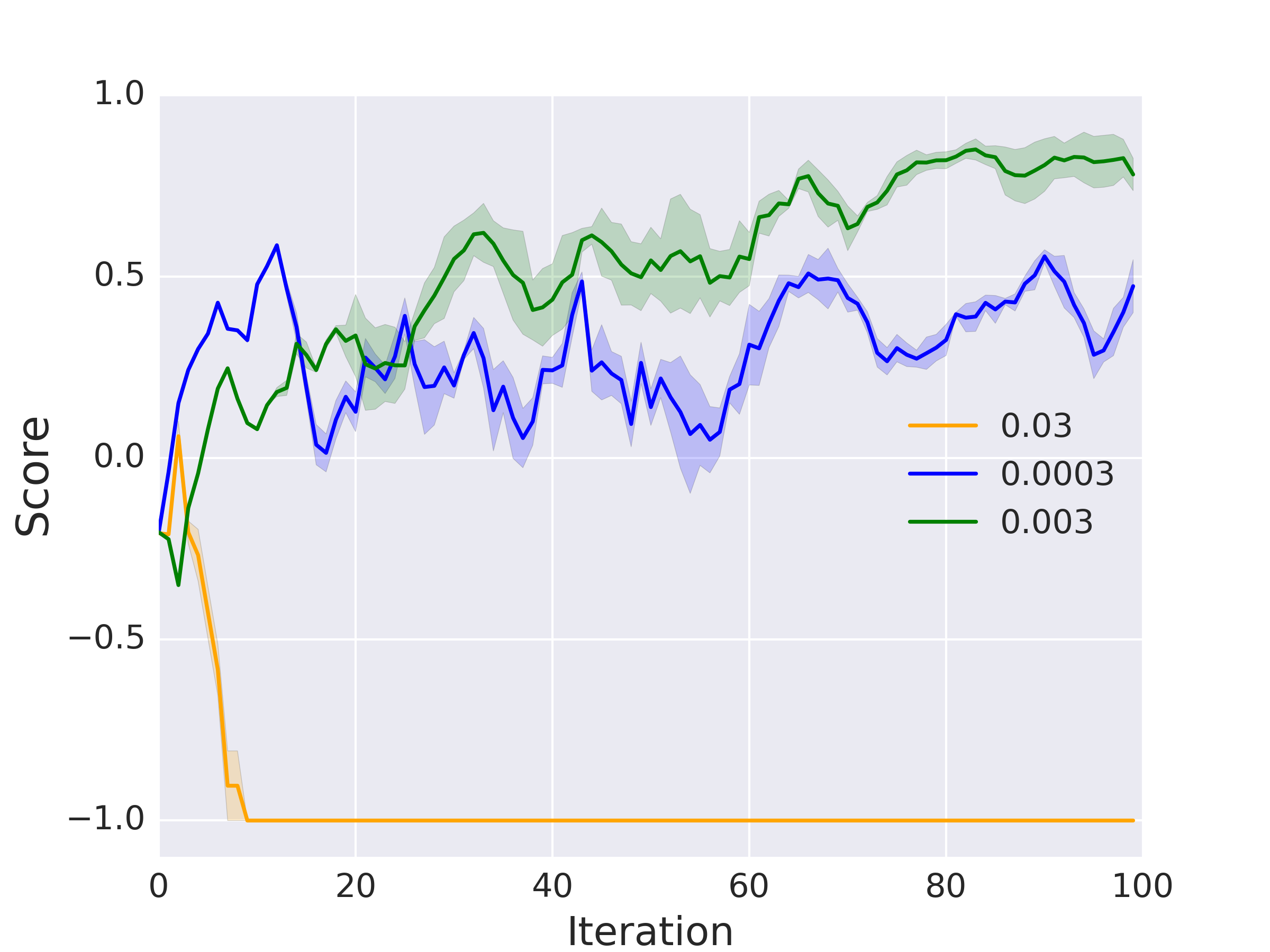
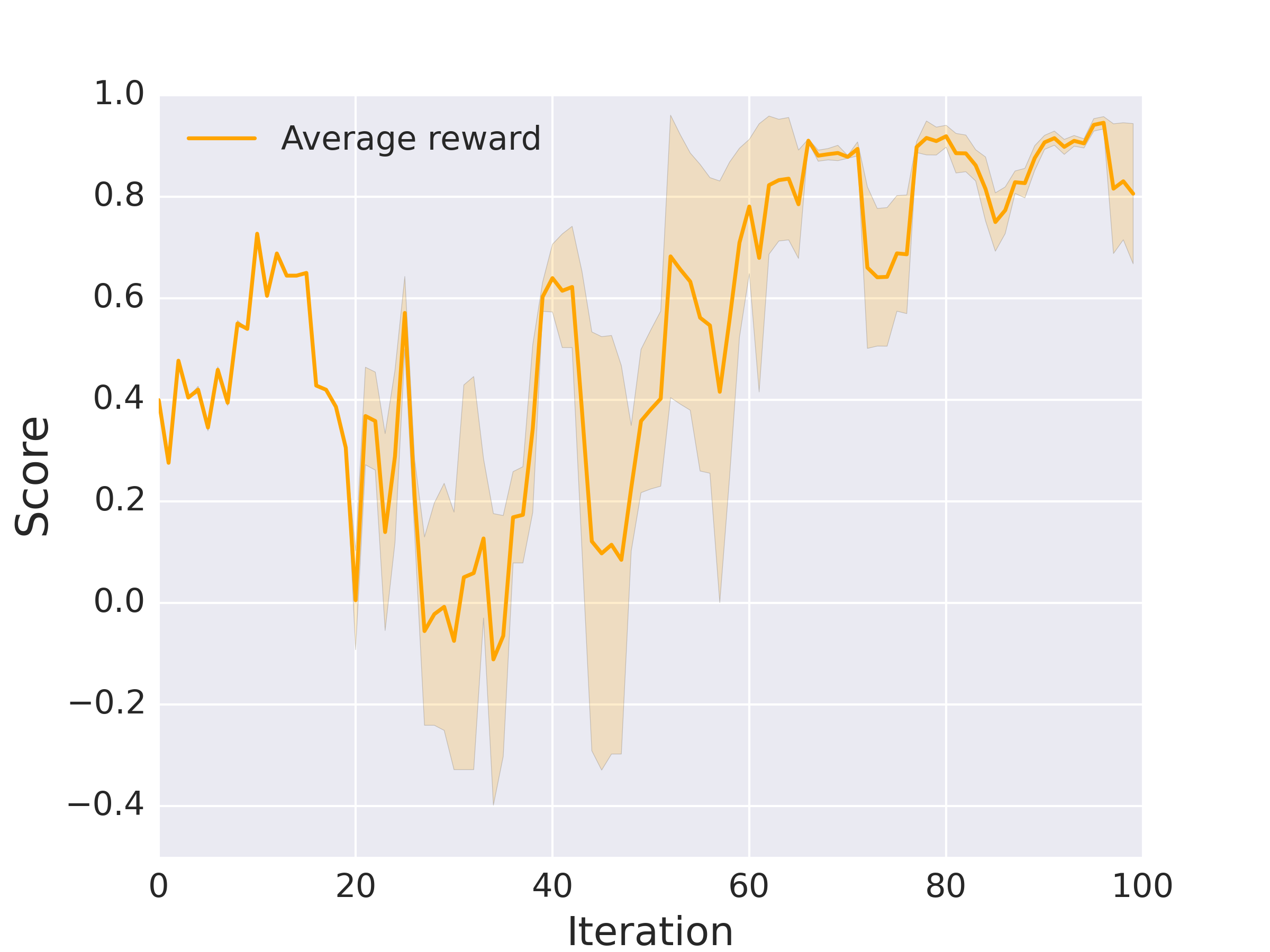
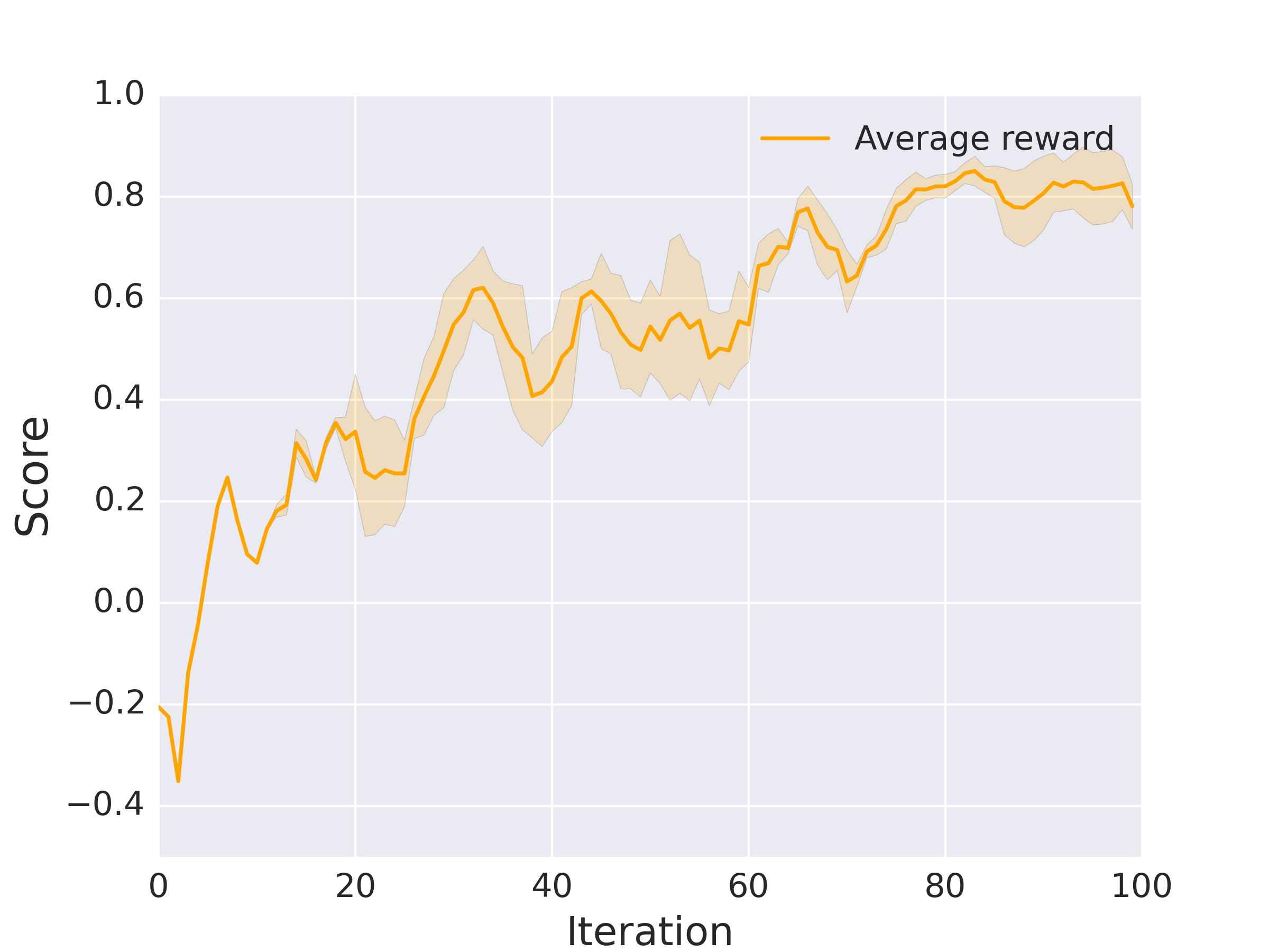
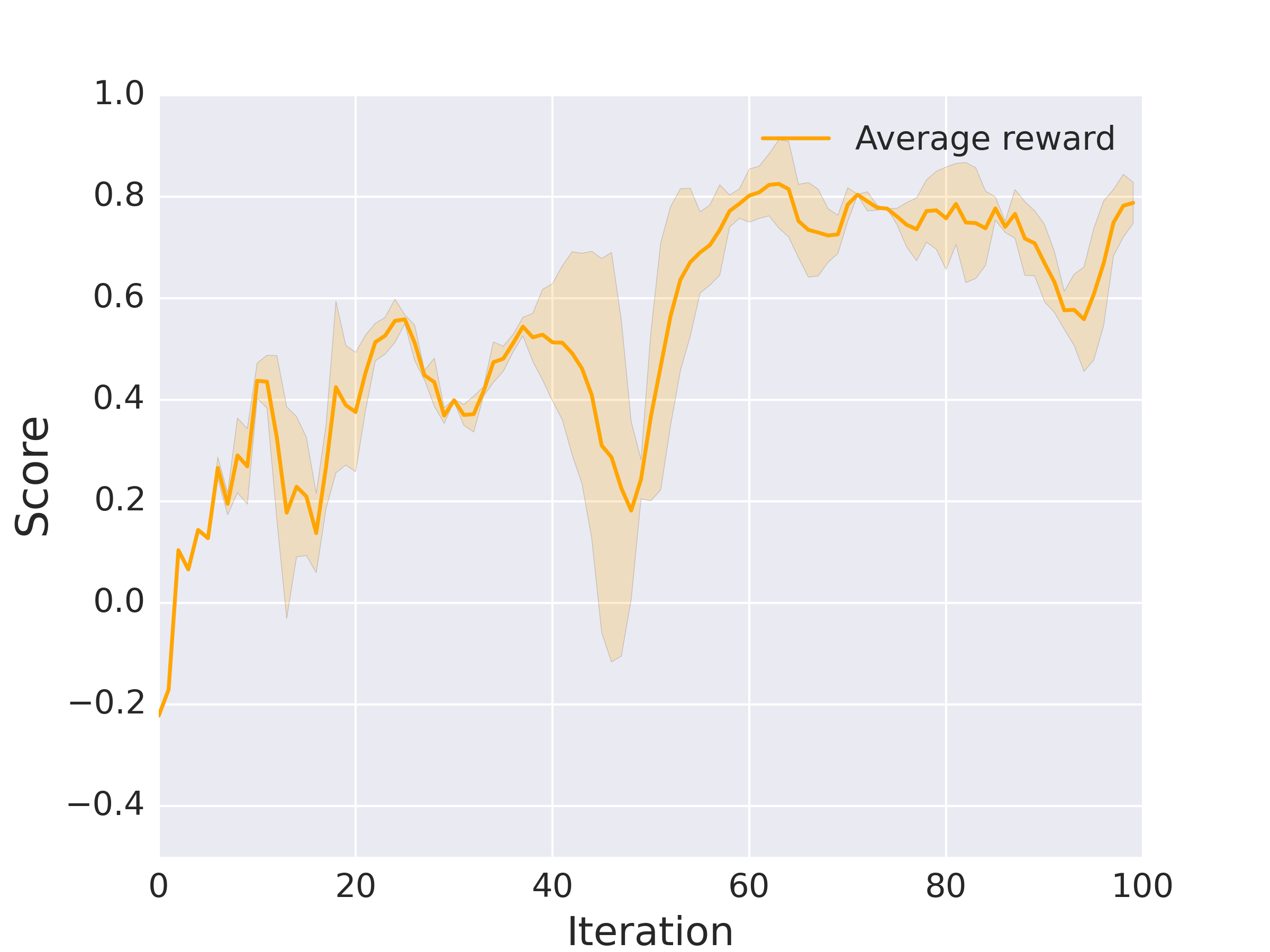
The learning rate and batch size were selected via a grid search. The following graphs show the rate of convergence for different learning rates and batch sizes.
7.1 Learning rate
In order to determine the learning rate, we performed a grid search over 0.03, 0.003, 0.0003. We performed this grid search on the MNIST dataset using the VGG-13 network to save time. For the stage-1 policy, it was observed that lr=0.03 did not converge while lr=0.0003 converged too slowly. Thus we used lr=0.003 as the learning rate.
7.2 Batch size
Similarly we performed a grid search to determine the optimal batch size over 1, 5, 10. A batch size of 1 was too unstable while a batch size of 10 offered no substantial improvements to justify the additional computation. Thus we observed that a batch size of 5 worked the best.
8 Transfer learning experiments
Below are the results of the transfer learning experiments, as observed, the pretrained policies start off with a high reward unlike the policies trained from scratch.
9 Additional experiments
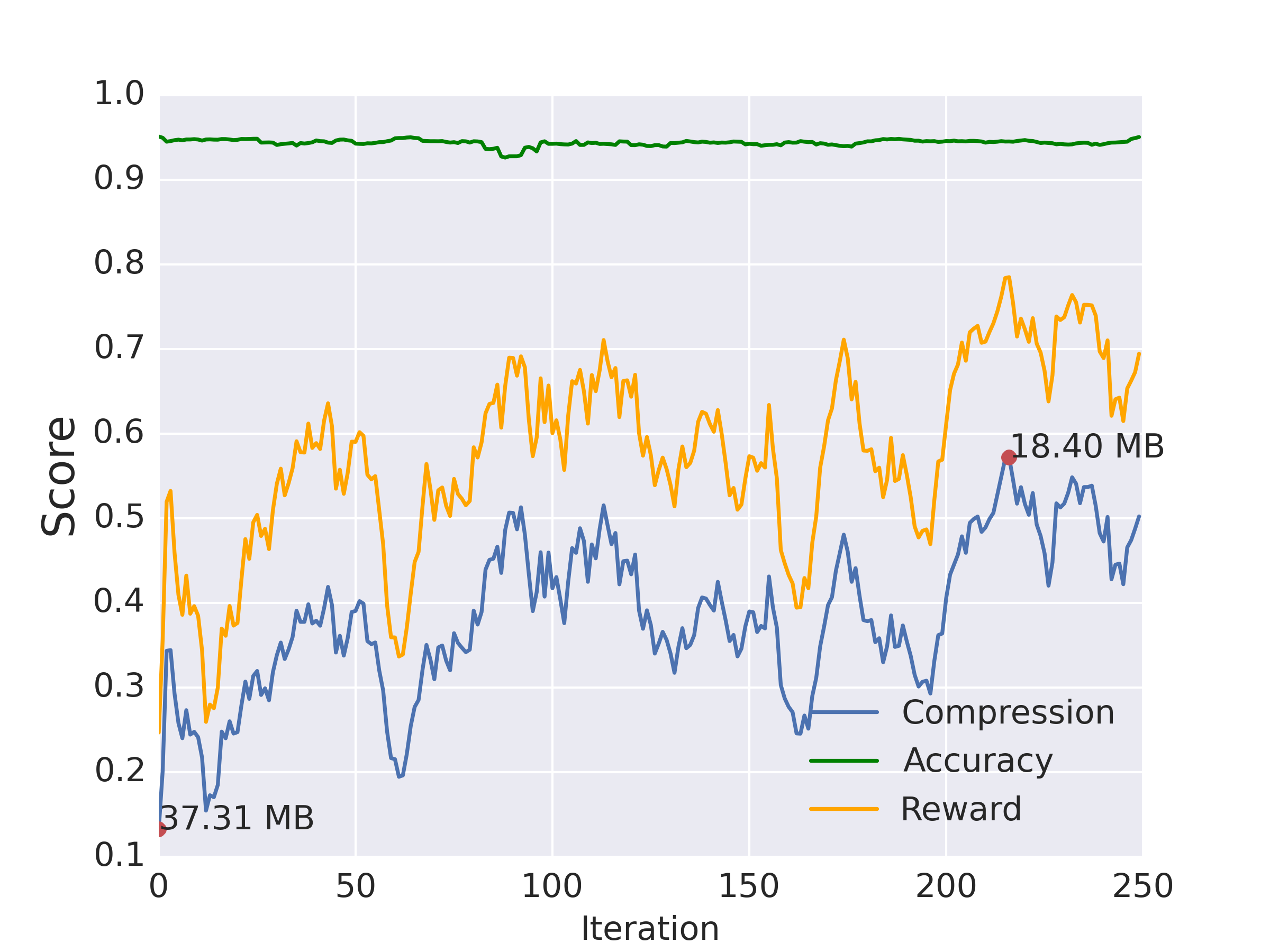
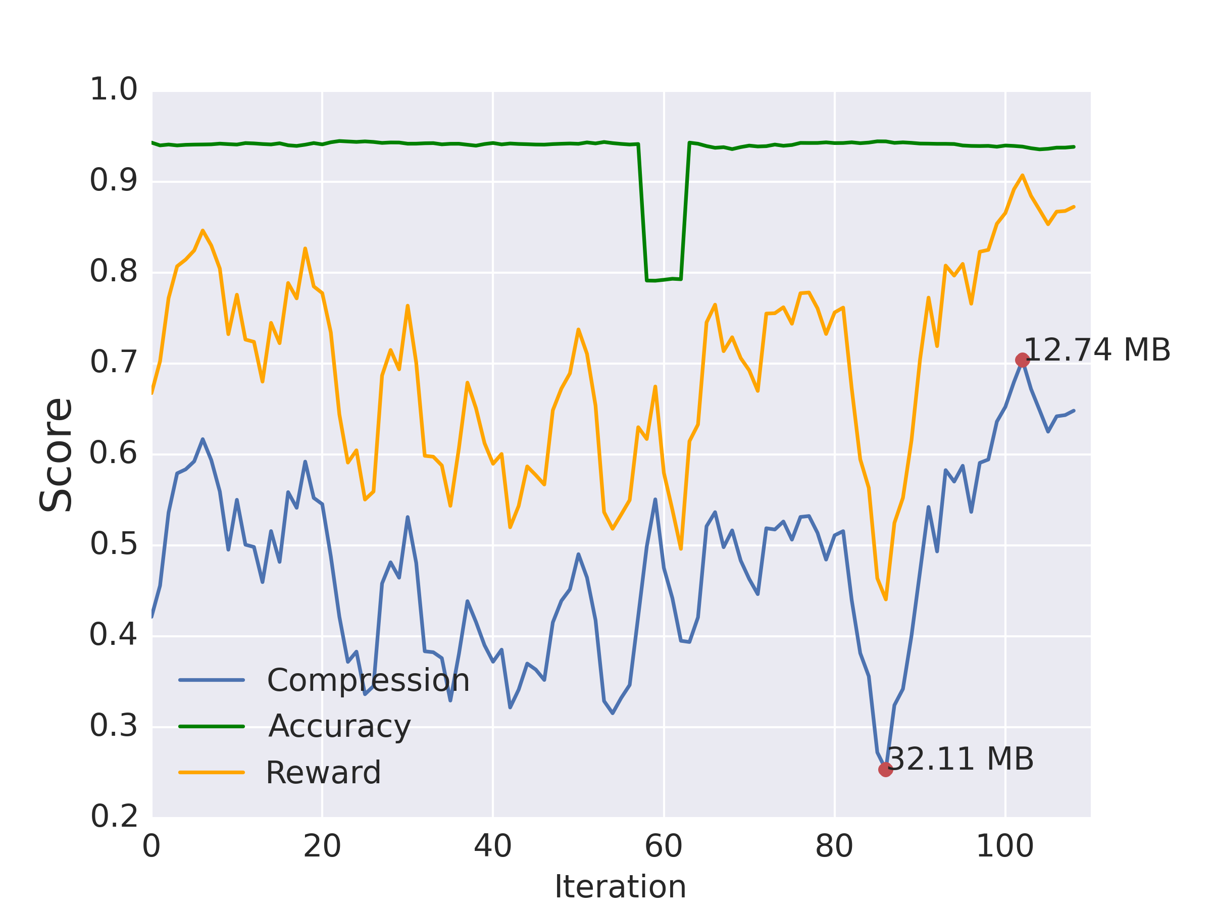
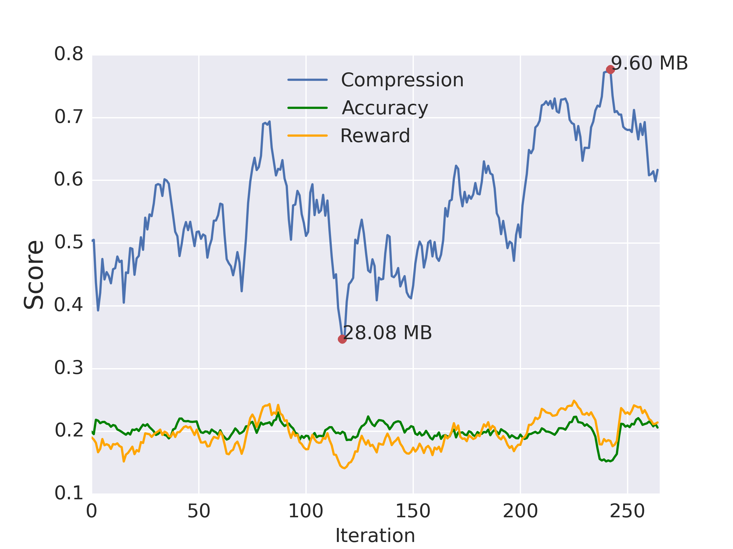
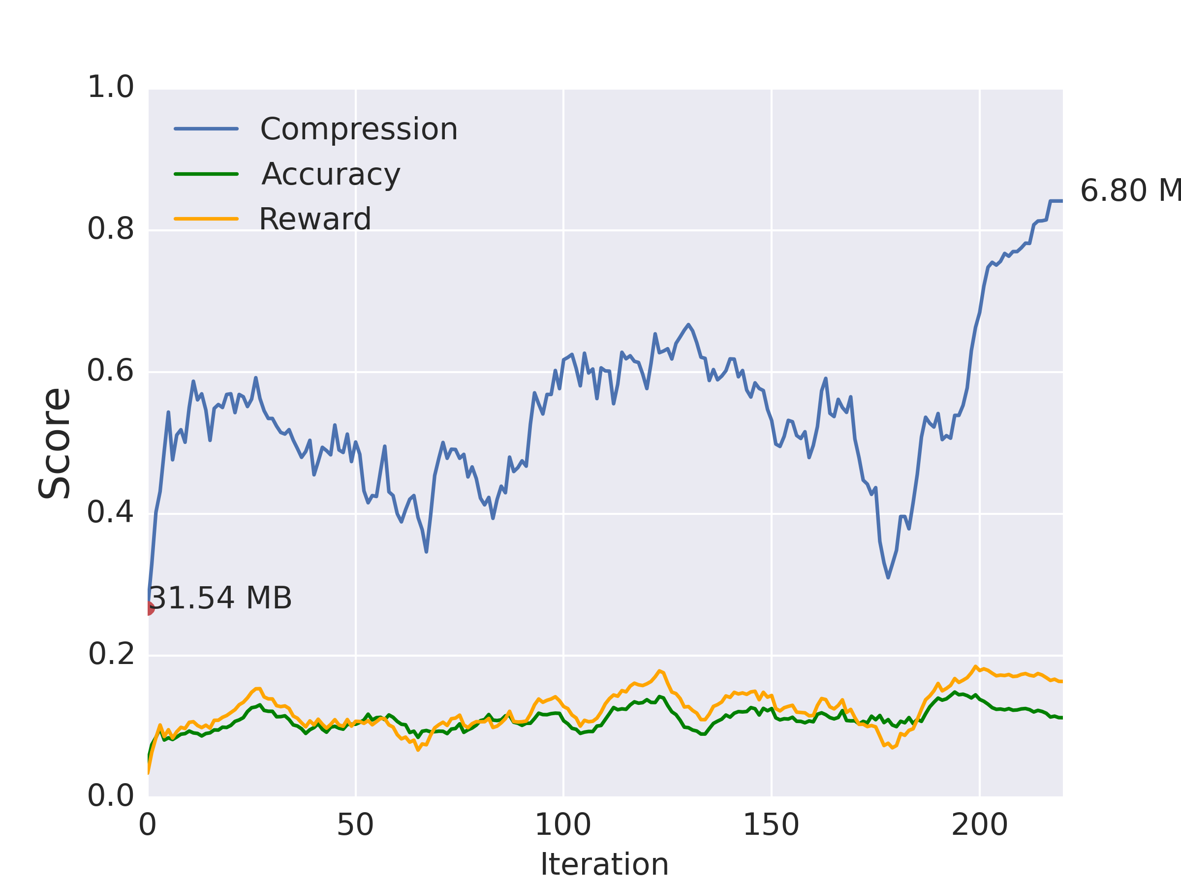
The following section contains results about additional compression experiments that were conducted.
10 Implementation details
The following section contains the implementation details required to replicate the experiments. All of the experiments were implemented in PyTorch with 4 NVIDIA TitanX GPUs.
10.1 Policies
Removal policy The removal policy was implemented with 2 hidden layers and 30 hidden units and trained with the Adam optimier and a learning rate of 0.003. The shrinkage policy was implemented with 2 hidden layers and 50 hidden units and trained with the Adam optimier and with a learning rate of 0.1. These policies were each trained for at least 100 epochs for each experiment. Batch size of 5 rollouts was used.
10.2 Teacher models
MNIST Teacher models for MNIST were trained for 50 epochs with a starting learning rate of 0.01. The learning rate is reduced by a factor of 10 in the 30th epoch. A batch size of 64 was used.
CIFAR-10/100 Teacher models for CIFAR-10/100 were trained for 150 epochs with a starting learning rate of 0.001. The learning rate is decreased by a factor of 10 in the 80th and 120th epochs. Standard data augmentation with horizontal mirroring (p=0.5), random cropping with padding of 4 pixels and mean subtraction of (0.5, 0.5, 0.5). A batch size of 128 was used.
SVHN Teacher models for SVHN were trained for 150 epochs with a starting learning rate of 0.001. The learning rate is decreased by a factor of 10 in the 80th and 120th epochs. Mean subtraction of (0.5, 0.5, 0.5) and a batch size of 128 was used.
Caltech256
To make the experiments controlled over alll datasets the Caltech256 models were trained from scratch. It is to be noted that Caltech256 models are usually initialized with pre-trained ImageNet weights since data is sparse. The training procedure consisted of 50 epochs with an intial learning rate of 0.01. It was reduced to 0.001 after the 50th epoch. Data augmentation such as horizontal flipping and random cropping alongside mean subtraction was used.
11 Reward design
In this section we go into greater detail regarding the design of the chosen reward function compared to a naive reward. For our objective of model compression, we want the reward to reflect the following qualitative heuristics.
-
1.
A model with compression but accuracy should be penalized more than a model with compression and accuracy. Since we do not want to produce highly compressed models which do not perform well on the task, we do not want to let the compression score dominate the reward.
-
2.
The reward function should montonically increase with both compression and accuracy.
11.1 Naive approach
Defining a naive, symmetrical reward function results in the following failure case. Suppose we define our reward as:
where are the relative validation accuracy and compression achieved by the student model. Let us consider the following 2 cases:
-
1.
accuracy, compression. A = 1, C = 0.25
-
2.
accuracy, compression. A = 0.25, C = 1
In both cases , which we do not want. If we use the reward function defined in the paper we get a reward of 0.25 and 0.4375 for each of the cases, which is closer to our true objective. In our empirical experiments, the non-linear reward outperformed the naive one. Other more complex reward functions that respect the above criteria may also work well.
The visualization of the reward manifold in 13 better illustrates the difference.
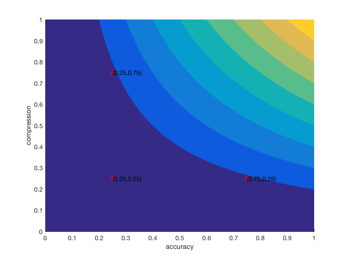
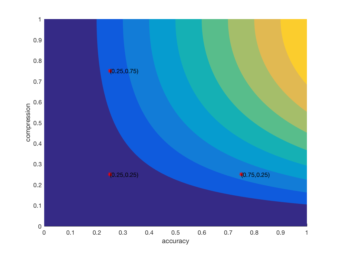
As observed, a naive reward function is symmetric while our reward function returns a lower reward for low accuracy, high compression models compared to high accuracy, low compression models. Both functions are monotonically increasing.
11.2 Degenerate cases
The following section outlines a few of the cases which are considered degenerate and for which a fixed reward of -1 is assigned.
-
1.
Empty architecture - Depending on how it is implemented, the policies could possibly output ”remove” actions for each layer during the layer removal stage. In this case, the output would be an empty architecture with no trainable parameters.
-
2.
Large FC layer - If too many layers are removed in the feature extraction portion of the convolutional neural network, the size of the feature map before the fully connected layers would be large. In this case, although we have a well defined reward, training the network could be impractical
-
3.
Specialized architectures - When dealing with more complex architectures, there may be inter-layer dependencies which impose certain requirements. For example, in a ResNet, the dimensionality of the feature maps at the start and end of each residual block has to match.
12 Future directions
This paper introduces a general method to generate an architecture that optimizes the size-capacity trade-off with respect to a particular task. The current limitation with this method is that we need to train each student model for a few epochs to determine a reward for it. This step can be computationally expensive depending on the dataset. Results from Saxe et al. (2011), Jarrett et al. (2009) and Cox & Pinto (2011) seem to suggest that initializing models with random weights could be an efficient way to evaluate architectures provided the right non-linearities and pooling are used. Another way to provide a better initialization could be to use a hypernetwork which takes the student model architecture as input and produces weights for the model. Other methods that select an informative subset of the training and test dataset to efficiently evaluate the network could also be interesting to explore. Another interesting direction would be to use the pretrained policies for transfer learning on different architecture search problems (apart from compression) to see if any generalizable information about deep architectures is being learned.