Backreaction and FRW consistency conditions
Abstract
If the FRW metric is a good approximation on large scales, then the distance and the expansion rate, as well different notions of distance, satisfy certain consistency conditions. We fit the JLA SNIa distance data to determine the expected amplitude of the violation of these conditions if accelerated expansion is due to backreaction. Adding cosmic clock and BAO expansion rate data, we also model-independently determine the current observational limits on such violation.
We find that the predicted maximum backreaction amplitude (95% C.I.) is of the same order as the current observational constraints , the precise numbers depending on the adopted fitting method (polynomials or splines) and stellar population evolution model. We also find that constraints on the value of determined from expansion rate data are sensitive to the stellar evolution model. We forecast constraints from projected LSST+Euclid-like SNIa plus Euclid galaxy differential age data. We find improvement by factor of 6 for the backreaction case and 3 for the model-independent case, probing an interesting region of possible signatures.
HIP-2017-22/TH
KOBE-COSMO-17-11
1 Introduction
Observations of the cosmic microwave background (CMB) and large scale structure show that the universe is statistically isotropic (with small anomalies [1, *Ade:2013nlj]), and they are consistent with the universe being spatially homogeneous [3, 4, 5, 6, 7] (see also [8, *Labini:2010aj, *Labini:2011tj, *Labini:2011dv]), in line with inflationary predictions. (See [12, 13, 14, *Stoeger1987, *Heavens:2011mr, 17, *Clarkson:2012bg, *Clifton:2011sn, 20, 21] for tests of the FRW metric and statistical homogeneity and isotropy.) A fundamental assumption in cosmology is that statistical homogeneity and isotropy imply that average properties of the universe over large scales are well described by the exactly homogeneous and isotropic Friedmann–Robertson–Walker (FRW) model. However, this is not necessarily the case: the effect of departures from exact homogeneity and isotropy on the averages is called backreaction [22, 23, 24, *Ellis:1987zz, 26, 27, 28]. It has been suggested that backreaction could explain late-time accelerated expansion [29, 30, 31, 32, *Rasanen:2004sa, 34]. In Newtonian gravity, the effect of inhomogeneity and anisotropy reduces to a boundary term [23]. In general relativity this is not the case, but backreaction on the expansion rate is small if the metric is perturbatively close to the same FRW metric everywhere [27] (see [35, *Green:2013yua, *Green:2014aga, *Buchert:2015iva, *Green:2015bma, *Ostrowski:2015pzb, *Green:2016cwo] for a related debate). It is not clear whether this holds in the real universe at late times. Backreaction effects have been started to be studied with relativistic cosmological simulations [42, *Adamek:2014gva, *Adamek:2014xba, *Adamek:2015eda, *Adamek:2016zes], including ones that are fully non-linear [47, *Bentivegna:2012ei, *Bentivegna:2013ata, *Adamek:2015hqa, *Bentivegna:2016fls] and without any symmetries [52, *Mertens:2015ttp, *Bentivegna:2015flc, *Giblin:2016mjp, *Bentivegna:2016stg, *Macpherson:2016ict, *Giblin:2017juu], but the magnitude of backreaction remains an open question.
In addition to changing the expansion rate, deviations from exact homogeneity and isotropy also affect light propagation. In particular, they modify the FRW relation between the average expansion rate and the angular diameter distance . This is a signature that cannot be mimicked by any FRW model (although extra dimensions can lead to a similar feature [59, *Ferrer:2008fp, *Ferrer:2009pq]). The FRW - relation can thus be used to test the FRW metric if the expansion rate and the distance are measured independently [12]. Similar tests can be made for the relation between the angular diameter distance and the parallax distance [62, 20], and the distance sum rule [21]. If backreaction is small, violation of the consistency conditions will be small. If backreaction is significant (in particular, if it leads to accelerated expansion), the degree to which the consistency conditions are violated depends on how the average expansion rate is modified. It can be argued that in a statistically homogeneous and isotropic universe the change of the - relation due to backreaction can be approximated by keeping the mapping between the redshift and the affine parameter the same in the Sachs optical equations (just substituting the average expansion rate for the FRW expansion rate) and replacing the source term with its spatial average [63, 64, 65, 66], although the issue requires more study. The source term depends on the matter content via the combination , where and are the energy density and pressure, respectively. This is not directly affected by a cosmological constant, so if matter can be approximated as dust and backreaction exactly mimics a cosmological constant plus FRW spatial curvature, i.e. the expansion rate agrees with the CDM model (which we take to include the possibility of non-zero spatial curvature), then the consistency conditions are not violated. Although there is at the moment no reliable calculation of the effect of inhomogeneity and anisotropy on the average expansion rate, there does not seem to be any reason for it to closely mimic the effect of a cosmological constant. In [67], the expected violation of the consistency condition was estimated with a toy model and a model-independent low redshift expansion to be . The consistency conditions have been observationally tested in [68, 69, 70, 21, 71, 72, 73, 74, 75], with deviations of this order of magnitude allowed.
The better the distance-redshift relation agrees with the CDM model, the smaller is the allowed violation of the consistency conditions. Turning this around, distance data can be used to determine how large violations are still allowed. If the maximum amplitude were to fall below the amplitude expected from backreaction by general theoretical arguments, this would be strong evidence against backreaction even in the absence of a precise prediction for the expansion rate.
We do a model-independent fit to the JLA dataset of type Ia supernova (SN) [76] to determine the luminosity distance , find the corresponding expansion history using the backreaction relation of [63] between and and calculate the predicted violation of the consistency condition. We also test the consistency condition using independent observations of and without assuming a theoretical model and compare to the prediction.
In section 2 we introduce the FRW consistency conditions and the backreaction equations, in section 3 we go over the data and in section 4 we discuss the fitting methods. In section 5 we give our results for the consistency condition both as predicted by the backreaction relation and as determined solely from observations, consider the value of implied by data and do a forecast for next generation data. In section 6 we summarise our findings.
2 Theory
2.1 FRW consistency conditions
If the universe (more precisely, light propagation on scales larger than the cosmological homogeneity scale) is described by the FRW metric and the geometrical optics approximation holds, certain consistency conditions relate the expansion rate and distance (as well as different notions of distance) to each other. These relations are purely geometrical, they are independent of the matter content and the dynamical relation between matter and spacetime (i.e. the Einstein equation).
The consistency conditions can be expressed in terms of the spatial curvature parameter that is constant in the FRW case. One condition relates the dimensionless expansion rate (where is the Hubble parameter as a function of redshift ; the subscript denotes present value throughout) and the dimensionless comoving angular diameter distance [12]:
| (2.1) |
where prime denotes derivative with respect to the redshift and the subscript indicates that the relation involves the Hubble rate.
Another consistency condition relates the angular diameter distance and the parallax distance [20]
| (2.2) |
where the subscript indicates that the relation involves the parallax distance.
A third condition can be derived from the sum rule between distances. In the spatially flat FRW case, the comoving angular diameter distance from to is simply the sum of the distance from to and the distance from to . In the spatially curved FRW case, the sum rule is more complicated, and the following combination is constant [21]
| (2.3) |
where the subscript indicates that the relation comes from the distance sum rule.
In a FRW universe, the three functions , and are constant and equal to minus the spatial curvature density parameter today, . If the spacetime is not well described by a FRW metric, they in general vary with and are different from each other. If it were observed that any of them depend on , or that any two of them are not equal, this would indicate that the FRW metric approximation is not valid. Observational constraints on have been reported in [68, 69, 70, 21, 72, 73, 74, 75] and on in [21]. There are currently no observations of the parallax distance over cosmological distances, and thus no constraints on , but this is expected to change with upcoming data from the Gaia satellite111http://sci.esa.int/gaia/ [20].
2.2 Backreaction
2.2.1 Redshift and expansion rate
Let us now introduce the relation between the distance and the expansion rate in the backreaction case. If matter can be approximated as dust and evolution of structures is slow compared to the homogeneity scale, it can be argued [63, 64, 28] (see also [77, 65, 66, 78]) that, analogously to the FRW case, the redshift is given by
| (2.4) |
where is the scale factor defined so that the volume of the hypersurface of statistical homogeneity and isotropy is proportional to , where is the time that is constant on the hypersurface. This relation depends on the cancellation of expansion rate fluctuations and matter shear along the null geodesic. The average expansion rate is , where dot denotes derivative with respect to .
The angular diameter distance can be solved from the Sachs optical equations. Assuming that null shear can be neglected and the Einstein equation holds, we have
| (2.5) |
where is the affine parameter, is Newton’s constant, and are the energy density and pressure, respectively, and is photon energy. We normalise the affine parameter as , where is photon energy at the observer. The dimensionless luminosity distance is [79, 80].
In the backreaction case, it can be argued that the average expansion rate gives the relation between the affine parameter and the redshift in the same way as in the FRW case, with the average expansion rate in place of the FRW expansion rate, , and the source is given by the spatial average, so (2.5) reduces to [63, 64]
| (2.6) |
where we have assumed that the matter can be approximated as dust (), and , where stands for spatial average. The initial conditions are , . The relation (2.6) differs from the FRW case with general matter content in that there is no pressure term on the right-hand side. Thus, if backreaction were to mimic the contribution of a cosmological constant plus FRW spatial curvature so that the expansion rate is given by , the distance would be the same as in the FRW case, and defined in (2.1) would have the constant value . Conversely, if backreaction changes the expansion rate in a different way, the distance will be different from the FRW case (where not only but also the right-hand side source term would change), and will not be constant.
Solving (2.6), we get in terms of ,
| (2.7) |
The FRW analogue of this equation is , solved from (2.1). (These two results agree if and only if the expansion rate has the CDM form given above.) In the FRW case, we need and the value of to determine . At first sight, it might seem that in the backreaction case has a similar role as in the FRW case. However, is not a free parameter. In realistic cosmologies, has a maximum, so for to remain finite, the zero of in the denominator must coincide with the zero of the numerator, which fixes .
We characterise the distance and the expansion rate with two effective equations of state. The effective expansion rate equation of state is defined as [67]
| (2.8) |
and the distance equation of state is defined in the same way, but substituting . The function is the total equation of state of matter in the spatially flat FRW model that has the expansion rate , and is the equation of state corresponding to the spatially flat FRW model with distance . If the universe is well described by the spatially flat expansion FRW model, we have , otherwise they will not in general agree. In the context of FRW models, it is more common to discuss the equation of state of a dark energy component alone rather than the total equation of state. However, if backreaction first slows down and then speeds up the expansion rate (or vice versa), the effective dark energy equation of state diverges at the transition. If backreaction explains the accelerated expansion, such evolution is expected [81, *Rasanen:2006kp, 67]. In fact, such a feature turns out to be common in model-independent fits to the real distance and expansion rate data, making it impossible to assign a finite effective dark energy equation of state, while the total equation of state is well-defined and finite.
2.2.2 Consistency conditions in the backreaction case
Given from the data, we determine from (2.7) and, using that together with , get from (2.1). Let us now find the expressions for and in terms of in the backreaction case. To express in terms of , we use the fact that the angular diameter distance from to satisfies the Sachs equation (2.5) for all values of , which correspond to different initial conditions. In particular, . As noted in [83], any two solutions of the Sachs equation (2.5) can be expressed (when null shear can be neglected) in terms of each other, and we can write
| (2.9) |
where is an integration constant. Taking a derivative of (2.9) and applying the initial condition , we get , giving us in terms of ,
| (2.10) | |||||
| (2.11) |
where on the second line we have used the relation . Given observations of , we can find from (2.7) and use these in (2.11) to find . Together with , we then get from (2.3).
For the parallax distance, we have [20]. Integrating, we get
| (2.12) | |||||
| (2.13) |
where we have on the second line again used , and fixed the integration constant to unity by comparing (2.2) and (2.7) around to next-to-leading order. The value of doesn’t matter for us, though, because the indefinite integral is not suited for numerical evaluation. However, noting that (2.12) involves the same integral as (2.10), we can write
| (2.14) |
where drops out. Expressing in terms of and using (2.2), inserting into (2.14) and comparing to (2.3) shows that . It immediately follows that if is constant, is constant and equal to . By using (2.2), (2.3) and (2.14), we can show that a constant also implies that is constant and equal to . If we assume , these conditions are also equivalent to being constant and .
3 Data
3.1 Distance from type Ia supernovae
We determine from SNe Ia light-curve data of the SDSS-II/SNLS3 Joint Light-curve Analysis (JLA) [76]. The catalogue includes light-curve parameters and their covariances for 740 SNe Ia in the redshift range . Another commonly used SNIa catalogue is Union2.1, which includes 560 SNe in the range [84]. The larger redshift range of Union2.1 would be an advantage in reconstructing the expansion rate (which requires determination of the zero of , which is typically at ) compared to JLA. However, in the Union2.1 catalogue the colour and stretch light-curve parameters are fixed through a fit to a reference spatially flat CDM model, and the covariance matrices necessary to marginalise over the related coefficients are not provided. Hence, if the data are used to fit different cosmologies, there is an unquantified model-dependence (see e.g. [85]). Analysis of mock data also suggests that the slightly larger redshift range would not make a significant difference for our results. We therefore use the JLA dataset only.
When determining the luminosity distance from the JLA data, we simultaneously fit cosmological parameters and the coefficients of the light-curve parameters. The JLA public dataset includes the light-curve parameters themselves (and their covariance) constrained using the SALT2 method [86] (which does not require an assumption about a cosmological model). The results depend on the modelling of the light-curves; for discussion of light-curve modelling and the impact of systematics on SNIa datafitting, see [87, *Li:2010du, *March:2011xa, *Lago:2011pk, *Giostri:2012ek, 92, 93, 94, 95, 96, 97]. The mapping of light-curve variation to the physical processes that the light-curve fitters model is not unique [98] and redshift-dependence of light-curve parameters can introduce degeneracy with cosmological parameters. Also, properties of SNIae depend on the host galaxies in a manner that is not completely understood and that has an impact on the inferred equation of state [76, 99]. There may also be residual model-dependence from correcting for selection biases [96].
Given these caveats, the interpretation of the precise results of SNIa data analysis requires caution, as demonstrated by comparison of light-curve fitters [87, *Li:2010du, *March:2011xa, *Lago:2011pk, *Giostri:2012ek] and datafitting methods [93, 94]. Nevertheless, such errors are not expected to change the qualitative picture and we are interested in the order of magnitude of the constraints rather than precise parameter estimates. Also, these errors are expected to be subdominant to the choice of how to determine and from the data model-independently.
3.2 Expansion rate from cosmic clocks and BAO
| [km/s/Mpc] | Method | |
|---|---|---|
| 0.070 | BC03 [100] | |
| 0.120 | BC03 [100] | |
| 0.179 | BC03 [101] | |
| 0.199 | BC03 [101] | |
| 0.200 | BC03 [100] | |
| 0.280 | BC03 [100] | |
| 0.32 | BAO [102] | |
| 0.352 | BC03 [101] | |
| 0.3802 | BC03 [103] | |
| 0.4004 | BC03 [103] | |
| 0.4247 | BC03 [103] | |
| 0.4497 | BC03 [103] | |
| 0.4783 | BC03 [103] | |
| 0.480 | BC03 [104] | |
| 0.57 | BAO [102] | |
| 0.593 | BC03 [101] | |
| 0.680 | BC03 [101] | |
| 0.781 | BC03 [101] | |
| 0.875 | BC03 [101] | |
| 0.880 | BC03 [104] | |
| 1.037 | BC03 [101] | |
| 1.363 | BC03 [105] | |
| 1.965 | BC03 [105] | |
| 2.33 | BAO [106] |
For an observational determination , we rely on measurements of galaxy ages and the baryon acoustic oscillation (BAO) pattern imprinted on large scale structure.
With a measurement of galaxy ages , it is straightforward to determine the expansion rate model-independently, as implies [108, 109, 110]. There are now several studies where is determined from observations of passively evolving galaxies [111, 104, 101, 100, 105, 103]. We use the data of [104, 101, 100, 105, 103], listed in table 1.222We do not use [111] due to concerns about the error determination [69]; see also the concerns of [112] regarding single stellar population models, which are used in [100]. Some of the dating methods rely on global spectral or photometric analysis [111, 104, 100], others use the 4000 Å spectral break [113, 101, 105, 103]. The absolute age is not always well fit by the models, but this is not a problem in itself, as depends only on the change of the age with redshift, and some systematic errors in the absolute age cancel out in the differential age [113, 103]333Ages inferred from the H Lick index are also systematically too high, possibly due to unsubtracted emission lines, and there the uncertainty extends to redshift evolution, making it impossible to use that feature for determination of [114].. At redshifts , the differential age determination depends significantly on the adopted stellar population synthesis model [101]. Some authors have chosen to add an extra 20% error to high- datapoints to account for this or drop some of the high- datapoints [115]. We instead consider the results of different population synthesis models, BC03 [116] and MaStro [117], and compare. However, it should be kept in mind that comparison of existing models (or simply increasing the error bars) does not necessarily account for the systematic effects, which can only be reliably settled by further study of the population synthesis models. (A similar caveat applies to differences between SNIa light-curve fitters.)
As the JLA dataset contains information only about the relative luminosity of SNe Ia, it can be used to obtain without worrying about the absolute normalisation of the distance. In contrast, to compare the observed data with the theoretical quantity , we also have to consider the normalisation factor . While there are increasingly precise determinations of using local SNe [118, *Riess:2016jrr, *Cardona:2016ems, 121, 122, 123], they are in some tension with the value extrapolated from determined from galaxy ages [124, 115, 125]. We therefore keep as a free parameter in the fit.
The BAO pattern and its distortion by the Alcock–Paczyński effect can be used to measure [126, 127, 128, 129]. We use the determinations of from the clustering of galaxies in SDSS-III BOSS [102] and the clustering of quasars in the Ly forest of SDSS DR12 [106], listed in table 1. The BAO observations constrain , where is the sound horizon at decoupling. We use the model-independent determination Mpc (68% C.I.), with [107]. The BAO data are not subject to similar astrophysical uncertainties as the SNIa and galaxy age data444However, see e.g. [130] for an example of a possible systematic error due to inaccurate modelling that may be a concern for more precise future observations., but the analysis is more model-dependent. The study is usually carried out in terms of non-observable comoving coordinates, requiring the assumption of a fiducial cosmology. While correction parameters are introduced to account for possible deviations from the fiducial model [131], it is not clear how well they describe models that are far from CDM. BAO analyses also rely on CDM mocks and the reconstruction technique applied to improve the statistics assumes CDM, so the precise error bars should be treated with caution. (See [132, *MiraldaEscude:2009uz, *Labini:2009ke, *Kazin:2010nd, *Cabre:2010bc] for discussion of early BAO observations.)
Given the systematic errors of the cosmic clocks and model-dependence of BAO measurements, we compare results from different data combinations. The differences are non-negligible, but within the large errors the overall conclusions are similar.
4 Fitting methods
4.1 Validation of numerical methods
We fit and model-independently with polynomials and splines, and also consider the CDM model for comparison. Other model-independent data fitting procedures have been used in the literature, most notably Gaussian processes [137, 115, 124, 125, 71, 75, 73]. However, the results of Gaussian processes depend on the choice of covariance function [138, 125] (see the discussion in appendix B). Other possibilities include non-parametric smoothing [68, 72, 74, 139], principal component analysis and genetic algorithms [70] as well as radial basis functions [140]. Numerical derivatives and binning have also been considered [69, 70], but being able to take analytical derivatives significantly improves precision (although possibly at the cost of accuracy).
Our computations are implemented in the Samp555Samp (Samp’s Adapted Monte Python) and other software used in this work are available under libre licenses at http://fmnt.info/projects/. code (based on Monte Python [141]). Curve fits are performed through Markov chain Monte Carlo (MCMC) methods to reconstruct Bayesian posteriors [142], based on the Metropolis–Hastings algorithm. As a convergence diagnostic for the MCMC chains (besides visual inspection of the chains traces) we require the Gelman–Rubin coefficient [143] to be . As a goodness-of-fit criterion we examine the reduced (with , given data points and fitting parameters) and, in the spline case, a cross-validation analysis (see appendix A). Unless stated otherwise, we consider flat uninformative priors except for the physical condition in the CDM case. The numerical methods are validated through a two-fold process:
-
1.
Unit tests are implemented for all main Samp functions related to polynomial and spline algorithms, prior to implementation into a specific likelihood code.
-
2.
The likelihood code is tested by fitting mock data obtained replacing the observed data points by corresponding ones for a spatially flat CDM model with and km/s/Mpc (with the same errors as in the real data). Such an analysis is repeated for each case.
For the study of consistency relations based on SNIa light-curve data, we also implemented the computation of the maximised profiles (i.e. the likelihood maximised in each MCMC histogram bin, also called a profile likelihood [144]) in Samp. Since MCMC methods may provide a poor description of the maximised profiles666A more easily computed quantity in MCMC analysis is the mean likelihood within each bin. However, it is not of relevant statistical interest aside from being a check of the robustness of results., we first compared a few results to those obtained with the robust Minuit minimisation algorithm [145]. More specifically, we used the Migrad algorithm included in the iminuit777https://pypi.python.org/pypi/iminuit Python package, based on SEAL Minuit2.888http://seal.web.cern.ch/seal/work-packages/mathlibs/minuit/ Results for the likelihood best fits are recovered well within the confidence intervals, which are themselves consistent at the level. This uncertainty on the errors does not affect our conclusions, hence the maximised profile analysis is carried out in Samp based on the MCMC chains, at the same time as the marginalised posterior analysis.
4.2 Supernova light-curve likelihood
Following the JLA analysis [76], the SNe Ia distance modulus is modelled as
| (4.1) |
where and are constants, and the -band peak magnitude and the Phillips colour and stretch corrections are obtained by fitting SN light-curves to photometric data, without having to specify the cosmology. To take into account dependence on host galaxy properties, the absolute magnitude is written in terms of the host stellar mass as
| (4.2) |
where and are constants and is the Heaviside step function.
The MCMC algorithm recovers the posterior distribution given the likelihood , where
| (4.3) |
where represents the JLA data vector (each component being identified by the corresponding redshift ) and the model is written in terms of the luminosity distance as
| (4.4) |
where we have introduced . For discussion of the contributions to the covariance matrix C, see [76]. The fit constrains the parameters that determine the functional form of the luminosity distance (polynomial, spline or CDM). As the JLA data contain no information about absolute luminosity, the parameter (which gives the normalisation of the luminosity distance ) used in the fit is fully degenerate with the absolute magnitude . Without loss of generality, we fix km/s/Mpc (corresponding to ) and marginalise over . (Note that this does not imply anything about the value of the physical Hubble parameter.) We are left with a total of four nuisance parameters , , and , which are constant over the sample and marginalised over. In practice, we find that , and depend only weakly on the cosmological model, and the values agree with [76]. The values of and agree with the ones in [98, 75, 74], and is slightly smaller than found for nearby SNe in [121].
When fitting the polynomials and splines to the distance data, has to satisfy certain physical conditions. We have the initial conditions
| (4.5) |
In addition, the Sachs equation (2.5) shows that . This means that only those parameters that lead to a distance with at most one extremum (which is a maximum) are physical. (Note that this does not imply .) The condition is equivalent to the statement that solved from the Sachs equation (2.7) is real, . These physical conditions are verified in Samp likelihood code on a fine redshift grid.
4.3 Expansion rate likelihood
When fitting to the expansion rate data, the posterior is recovered given the likelihood , with:
| (4.6) |
where denotes the expansion rate data at a given redshift , are the respective errors and we have the boundary condition
| (4.7) |
The data provide , so we also vary as a free parameter. (This corresponds to the physical expansion rate today.)
4.4 Fitting functions
4.4.1 Polynomial
We use a fourth order polynomial to fit the luminosity distance :
| (4.8) |
where the coefficients are varied to fit the JLA distance modulus . The homogeneous and linear coefficients ( and ) are fixed by the initial conditions (4.5). The polynomial order is set through mock data analysis, selecting the lowest order that provides fits accurate enough for our purposes. We tested with mocks also fitting a polynomial to or instead, but the luminosity distance proved to be the most accurate. (For discussion of different distances, see [146, *Visser:2009zs].)
The Hubble parameter is modelled with a second order polynomial:
| (4.9) |
The homogeneous coefficient is set by the initial condition . Again, the order of the polynomial has been chosen to be the lowest that provides sufficiently accurate fits to mock data.
4.4.2 Spline
To fit spline functions we first set knots , where , with and the rest logarithmically distributed over the data redshift range. The corresponding luminosity distance values are free parameters, except for . We interpolate the points , where , with cubic splines so that the distance at a given redshift (within the interpolation range) is given by the spline algorithm:
| (4.10) |
The parameters of the fit are for . We impose the boundary condition on the derivative at the first knot, as required by (4.5), and marginalise over at the last knot. This last requirement leads to a better determination of the first derivative of the distance at large redshifts compared to the polynomial fit case. For the Hubble parameter, we take and set second derivatives at the boundaries using natural spline conditions .999Marginalising over the derivatives at the Hubble parameter boundaries would only slightly increase errors without affecting our results. In contrast, arbitrarily fixing the derivative of the distance at the end point would introduce a non-negligible systematic bias, hence we marginalise over it. The rest of the analysis is done in the same way as for the distance fit.
The number of spline knots must be large enough to allow a good fit, but sufficiently small to avoid overfitting. Based on mock data analysis, we set for the luminosity distance and for the Hubble parameter. Increasing the number of knots does not improve the goodness-of-fit. Setting the knots on a linear (as opposed to logarithmic) scale in redshift would require a larger number of knots to reach a comparable fit. As a further check against overfitting, we also introduce a roughness parameter, whose value is set by a cross-validation analysis, described in more detail in appendix A. The results indicate that the selected number of spline knots does not overfit the supernova nor the Hubble parameter data.
4.4.3 CDM
In the CDM model, the Hubble parameter at late times is
| (4.11) |
with , and the set of varying parameters is and .
In this case, the distance can be solved from the Sachs equation (2.5) in closed form,
| (4.12) |
4.4.4 Derived functions
The polynomial, spline and CDM fits provide the uncertainties on the respective parameters used to model the luminosity distance and the Hubble parameter. However, we are not interested in the fit parameters themselves, but on the error contours of functions of those parameters. Specifically, we want to find the distance , Hubble parameter ,101010Spline fits already directly provide distances and Hubble parameters at the respective redshift knots, but we are interested in recovering such functions (and others) at any arbitrary redshift within the data range. consistency condition functions , , and the equations of state and . To estimate error contours, we compute a given function (at a fixed redshift value ) for each point of the MCMC chains. Error contours are then easily computed at each redshift (in practice we only consider a few redshift values). In the interpretation of the results, it should be kept in mind that there are non-trivial correlations between different redshifts, as discussed in appendix B.
Unless otherwise noted, we quote error bars as 68% C.I. and limits as 95% C.I., the expression “C.I.” referring to confidence intervals for maximised statistics and minimum credible intervals for marginalised statistics (see appendix C for details); the meaning should be clear from the context.
4.5 Distance selection bias
When we determine the backreaction expansion rate from (2.7), we are faced with the issue that the denominator of (2.7) vanishes at where , as noted earlier. Therefore, for curves with a maximum, the value of has to be chosen such that the numerator vanishes at the same redshift. This leads to two problems.
First, is typically somewhat larger than the maximum redshift in the data, so the value relies on extrapolating the fit. Spline fits cannot be extrapolated, so we only consider polynomials here. The extrapolation is not large, as is typically not far outside of the data range (in the spatially flat CDM model with , the value is ), and mock data analysis suggests that the recovered values are consistent with the fiducial cosmology. Fitting Union2.1 data, which go to slightly larger redshifts () than JLA () or adding a distance data point at from Ly BAO analysis [148] would not substantially affect the conclusion, while increasing model dependence.
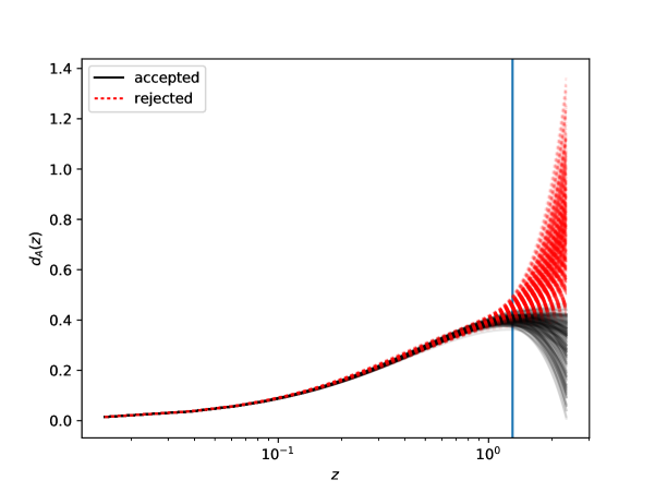
Second, and more important, not all curves that provide a good fit to the data have a maximum, as shown in figure 1. We reject such curves (some of them would lead to , a symptom of not satisfying the condition ). Redshifts beyond the JLA range () are not considered in the , but we extend the search for the maximum up to . This is a good compromise between including well-fitting curves with but not considering too large redshifts, where the extrapolation of the polynomial becomes unreliable. The cutoff redshift is somewhat arbitrary, but the results are not very sensitive to the its precise value; for example, choosing instead does not change the results. Mock data analysis shows that the selection effect of demanding to have a maximum in this range causes significant bias in the marginalised statistics, but not in the maximised statistics. We discuss this in more detail in appendix C. If we did not demand to have a maximum, some of the curves would still have to be discarded because they would lead to .
In summary, when determining the backreaction case from the distance data, we require to have exactly one maximum (in order to set such that is positive and non-singular), and focus on maximised rather than marginalised profiles.
5 Results
5.1 Expansion rate and consistency conditions from backreaction
5.1.1 Distance and expansion rate
We first determine the luminosity distance from the JLA data, then find the corresponding backreaction with (2.7) and calculate the allowed range for , and .
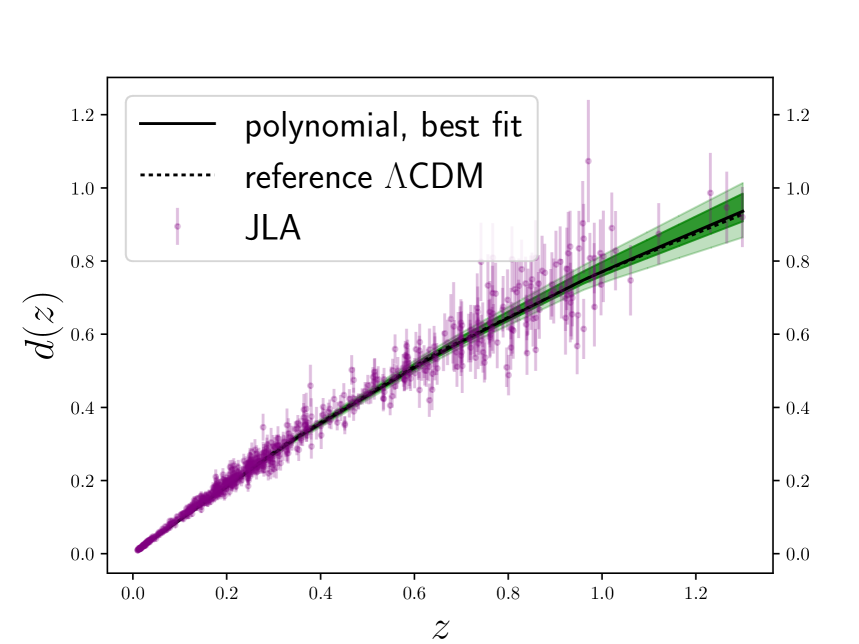
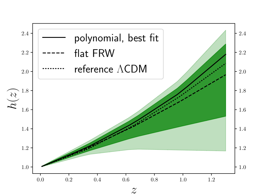
Figure 2 shows the results obtained by fitting the polynomial luminosity distance to the JLA SNIa data. The data points shown are obtained by fixing the nuisance parameters to their best fit values. The distance is relatively well constrained: the polynomial best fit, shown in figure 2(a), is close to the CDM best fit, and the 95% contours are quite tight, with only 10% errors even at the largest redshift. The result for the matter density determined from the maximum of , , is close to the result for the CDM model fitted to the same JLA data, . In contrast, the Hubble parameter determined from (2.7), shown in figure 2(b), shows large errors at high redshifts, in part due to the spread in values determined with the extrapolation. In addition to the backreaction and CDM curves, we show the curve corresponding to the polynomial best fit distance in a spatially flat FRW model, where . It shows a clear difference from the backreaction case, of order 10% at high redshift, suggesting significant violation of the FRW consistency condition (though it has to be checked whether this could be fitted by FRW spatial curvature). However, the difference is completely swamped by the large errors. The errors could be reduced by adding an angular diameter distance determination at from Ly BAO analysis [148], but this would increase model dependence without changing the main conclusions. The errors are smaller at low redshifts due to a better determination of the distance, combined with the initial conditions at .
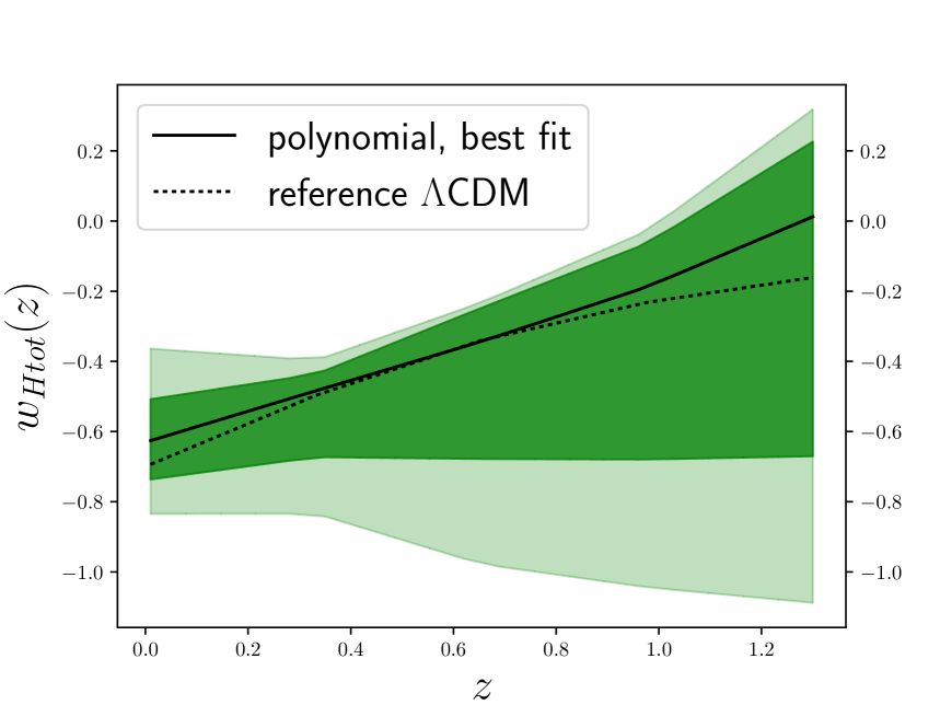
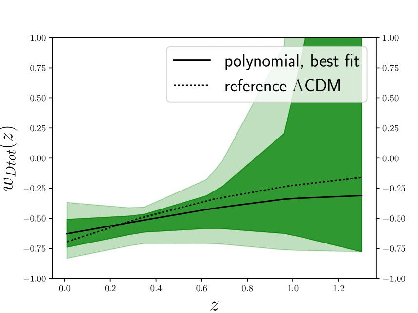
The uncertainty in the total equations of state and , shown in figure 2, is even larger, and they are consistent with each other. This is not surprising, as the equations of state depend on the second derivative of the distance, and even small errors in the distance can lead to large errors in the equation of state [149], as our mock studies confirm. At large redshift, the errors are much larger for than for . This is mainly due to the fact that the values are determined to provide a finite from (2.7), which then enters in . Instead, depends on , which is more affected by the spread in distance values introduced by the extrapolation. While increasing the polynomial order leads to more precision in the derivatives, it does not necessarily increase accuracy due to overfitting and the fact that in general higher-order polynomials do not provide a more reliable extrapolation (used to determine ).
5.1.2 Backreaction prediction for
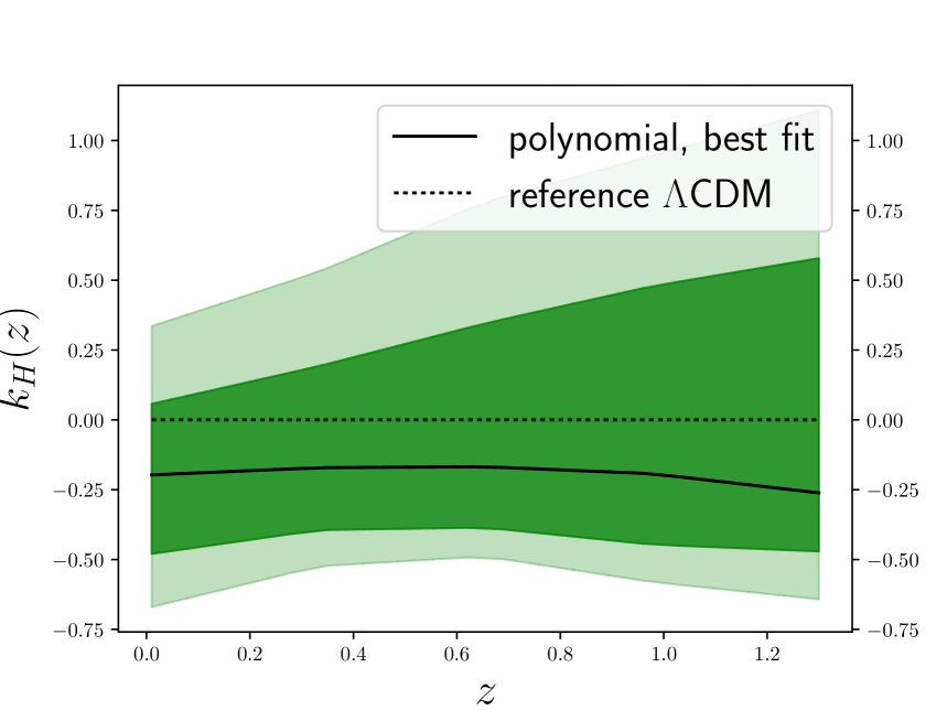
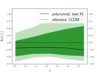
We input the determined from the JLA data and the corresponding calculated from (2.7) into the expression (2.1) for : the result is shown in figure 2(e). In contrast to the effective equations of state, depends only on the first derivative of , though it is still affected by the spread in . The best fit shows a clear deviation from the spatially flat FRW case, with for the whole data range. This is the same order of magnitude as obtained in [67], where a backreaction toy model was fitted to the data, but the redshift-dependence is completely different. The fit result is almost constant, reflecting the fact that the distance data does not require the kind of features in that are expected if backreaction explains the accelerated expansion (such as early extra deceleration and possible late transition from acceleration back to deceleration). Because is almost constant, it would be difficult to distinguish backreaction from FRW spatial curvature using observations at redshifts . However, the behaviour at high redshifts would be completely different, as the FRW constant has a large impact on the distance to the last scattering surface (which is precisely constrained model-independently [150, *Audren:2013nwa, 141]) unlike a backreaction , which would be expected to rapidly decrease for as the effect of non-linear structures becomes negligible [67]. In any case, there is no detection of any deviation from the FRW case and within the error bars it is not possible to make out any trend of redshift evolution. The large errors still allow for features in , with the 95% confidence contours covering the range , though because of large correlations between different redshifts (see appendix B for details) it is not possible to put constraints on them simply by considering figure 2(e). The tightest constraint is at .
This result shows how much deviation from the FRW consistency condition is expected given the observed light-curves, if backreaction is responsible for the accelerated expansion and the relation between the average expansion rate and distance is given by the relation (2.7). Before comparing this to what the combination of distance and expansion rate observations gives for , let us also find the backreaction range for and .
5.1.3 Backreaction prediction for
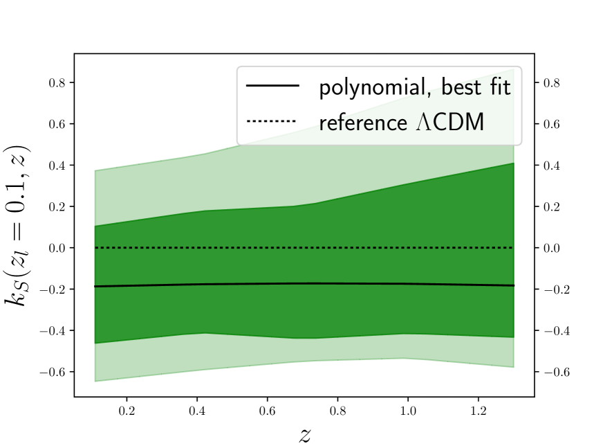
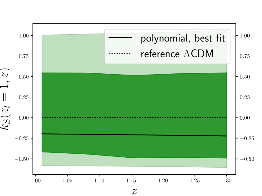
The backreaction sum rule consistency condition function is determined from the polynomial fit to the observed by first finding from (2.7), determining from (2.11) and inputting them together into (2.3). The result is shown in figure 3. In the two plots we show the cases where is 0.1 or 1.0. The best fit goes slightly down with , and the errors increase with larger , because the distance is more poorly determined. The dependence on is small: in both cases the best fit prediction is almost a straight line, the errors just increase slightly.
5.1.4 Backreaction prediction for
As , and the best fit is close to constant in both redshift variables, this implies that the best fit is also close to constant, as we indeed see in figure 4. For the best fit, , and the error contours are similar as for . If one of the consistency condition functions were strictly constant, they would all be constant and equal to each other, so it is not surprising that as they are (for the best fits) almost constant, they are also close to each other. In fact, the contours for and are essentially indistinguishable. However, the 95% C.I. contours cover a wide range of possible values and redshift-dependencies.
There are no observations of the parallax distance on cosmological distances at the moment, but upcoming data from the Gaia satellite may yield a constraint of the order , provided that there will be measurements of at the corresponding redshifts [20].
5.2 Distance, expansion rate and consistency conditions from the data
5.2.1 Fits to the distance data
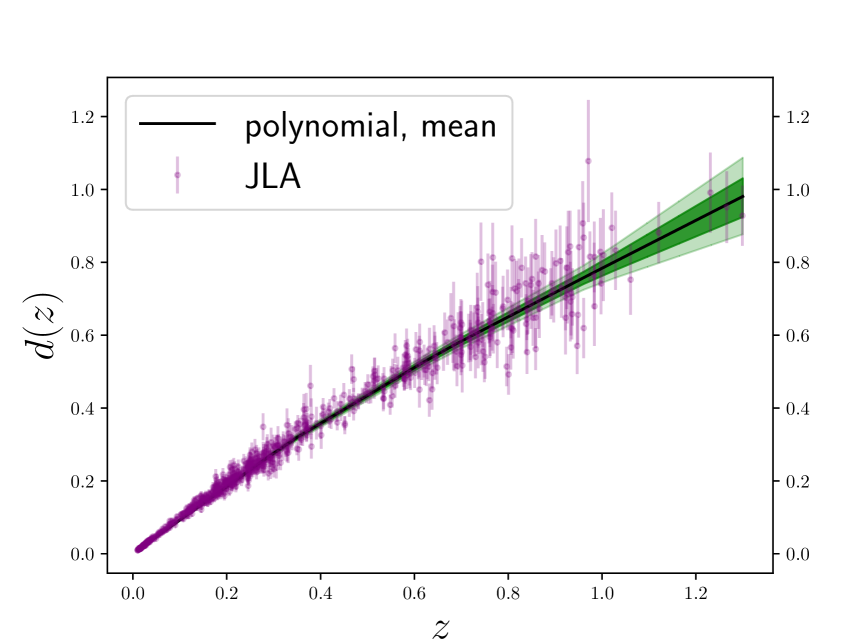
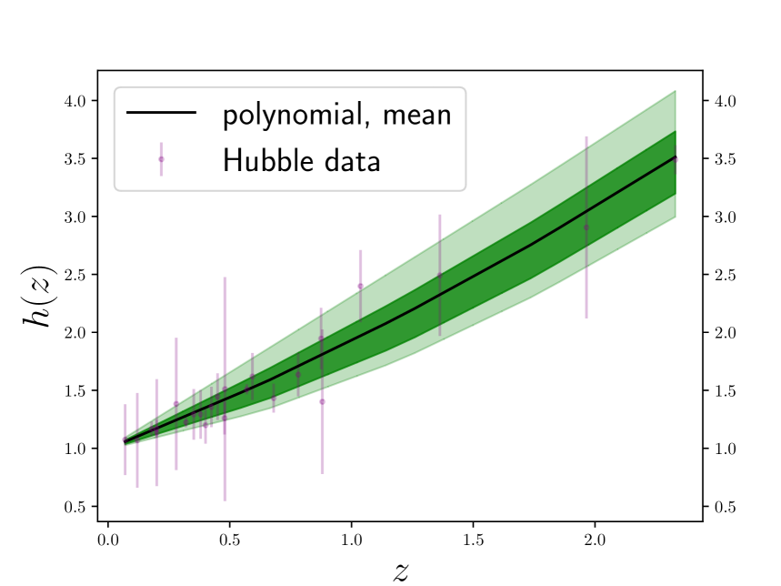
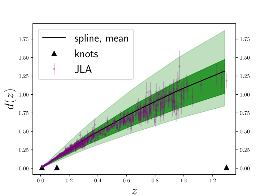
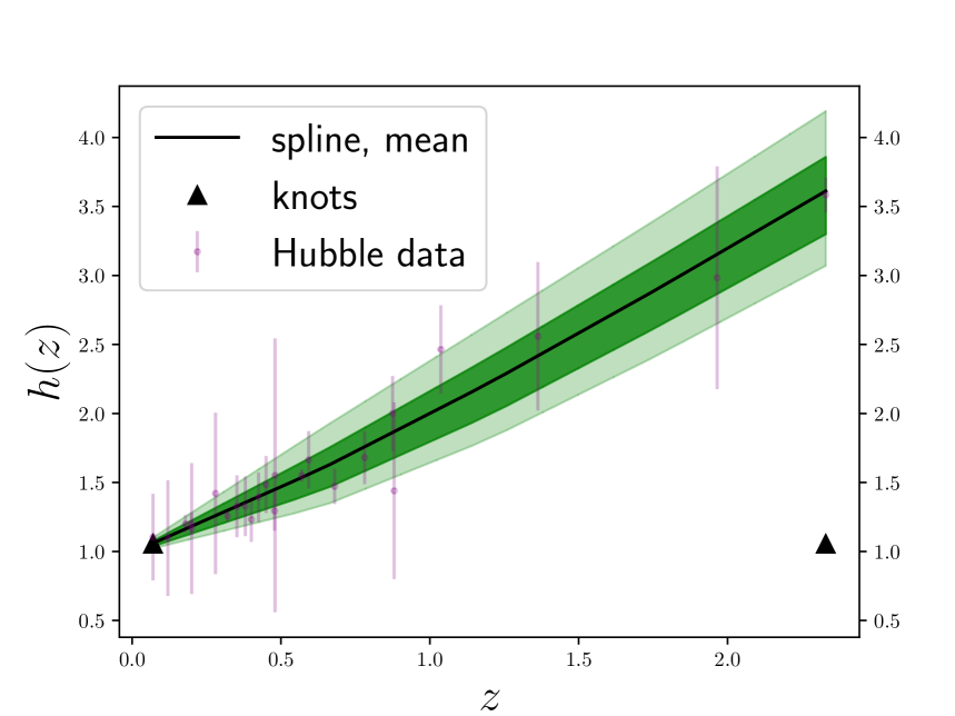
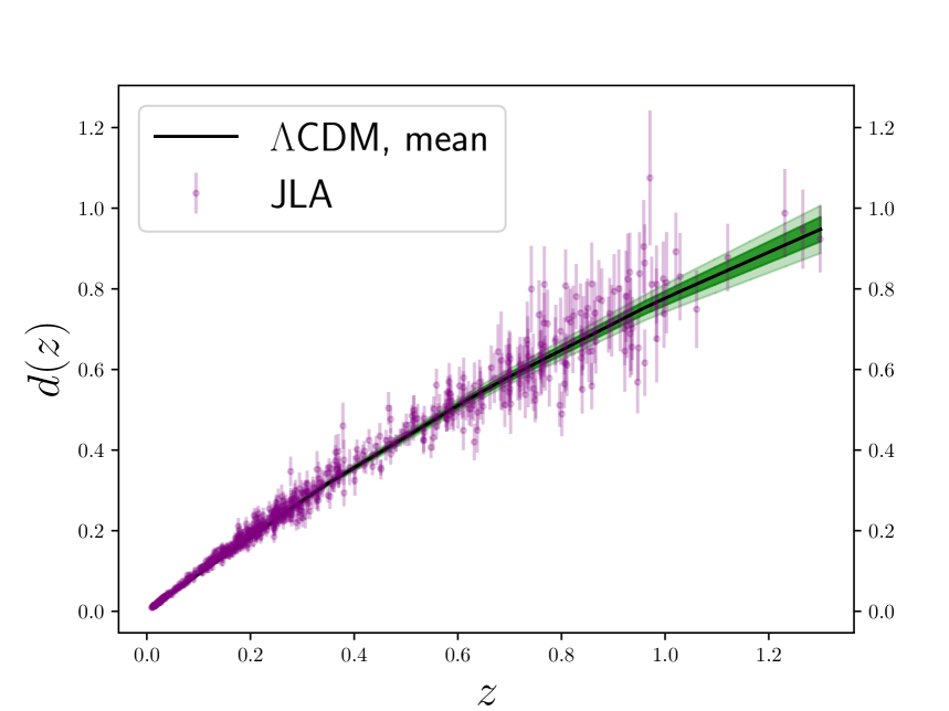
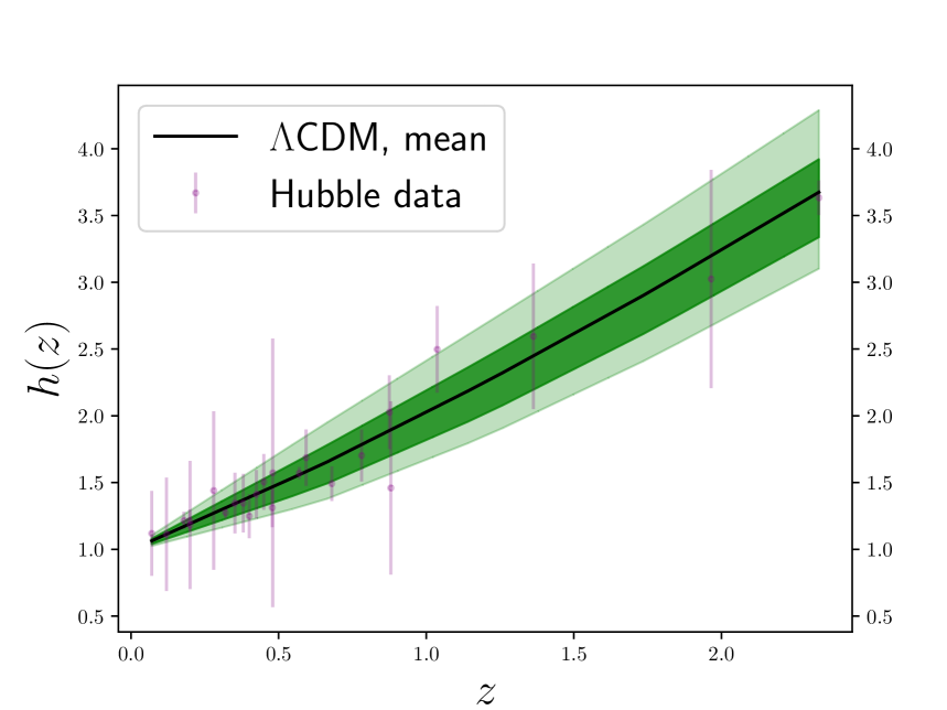
We now move to determining the expansion rate and the consistency condition from the data alone, without backreaction assumptions. In this case, there is no need to look for the maximum of , so we consider both polynomials and splines to get a handle on the dependence on the fitting function, and again consider the CDM model for comparison. Figure 5 shows the distance for these three cases. As before, the data points shown in the plots are obtained by fixing the nuisance parameters to their mean values. In the spline case we also show the location of the knots corresponding to the distance values varied in the chain (the knot at , fixed by the initial conditions, is not shown).
The three fitting functions give values that are comparable, though slightly larger for splines. Compared to the polynomial, the spline fit accommodates a wider variety of distances at the same confidence interval (only in small measure due to the fact that marginalisation over the final spline boundary condition involves a further nuisance parameter), and the CDM model is of course even more constrained than the polynomial. Otherwise the recovered distances are qualitatively similar, the spline result favouring somewhat longer distances. For the splines, the posterior mean differs from the global best fit by at lower redshifts. This is caused primarily by degeneracies in parameter space leading to a volume effect with respect to in the marginalised constraints, similar to the degeneracies in the backreaction case discussed in appendix C. Mock analysis shows that if is fixed to its best fit value, the mean of the distance correctly recovers the expected value. As a result of this degeneracy, the derivatives of the distance are not well recovered. Adding more spline knots does not improve the situation, because in this case the Metropolis–Hastings algorithm is not an efficient enough sampling in the direction (alternatives such as Nested Sampling, Hamiltonian/Hybrid Monte Carlo or other techniques could be more appropriate, see e.g. [152] and references therein).
5.2.2 Fits to the expansion rate data
Fits to BC03+BAO Hubble parameter data are shown in figure 5. In this case all fitting functions give similar results. The narrow error contours at small redshifts are partly due to the initial condition . The Hubble parameter is better constrained at high redshifts than the backreaction prediction shown in figure 2(b) (note the different redshift ranges of figures 2(b) and 5), because in the backreaction case depends on determination of using the zero of , which introduces extra spread. Within the errors, the expansion rate does not show any features. It should be noted that our second order polynomial (or two free spline knots) may not have the flexibility to fit features, but the choice reflects the fact that the present data are not very constraining. For results for other fitting methods, see [124, 115, 153].
Fits to BC03 data are characterised by small due to large errors. The optimal fit parameters have been tested through cross-validation to rule out flagrant overfitting. Datapoints obtained with MaStro stellar modelling give a more reasonable and are overall consistent with BC03. However, these goodness-of-fit values should be interpreted with caution. We expect fits to both BC03 and MaStro to be poorly predictive due to large errors and small amount of data. For instance, adding just three precise BAO data points helps to improve the goodness of fit in both cases, though the overall conclusions are unchanged as the errors are in any case large.
| [km/Mpc/s] | BC03 | BC03+BAO | MaStro | MaStro+BAO |
|---|---|---|---|---|
| polynomial | ||||
| spline | ||||
| CDM |
In table 2 we show the value for different fitting functions and datasets. The values are consistently lower than determinations from nearby SNe Ia (which have mean values from 72.5 to 73.75 km/s/Mpc and 68% C.I. ranges from 1.7 to 3.2 km/s/Mpc, depending on the analysis) [118, *Riess:2016jrr, *Cardona:2016ems, 121, 122, 123], although our error bars are large. (The exception is the MaStro only data, which consists of only 8 points, and for which the errors are particularly large.) This is in agreement with previous determinations of from data [124, 115, 125]. The differences between fitting functions are within the 68% C.I. (the effect of different fitting functions was investigated in the context of Gaussian processes in [138, 125]), whereas the differences between stellar evolution models are larger, suggesting caution in the interpretation of the value of derived from cosmic clock data.
The determination of from local SNe is not independent of cosmology, it depends on the value of the deceleration parameter via the series expansion of . As discussed in [123], more positive values of (meaning less acceleration today) give smaller values of . If backreaction explains the accelerated expansion, the acceleration is transient and the expansion will at some point start to decelerate [81, *Rasanen:2006kp]. The distance data are consistent with (but, obviously, do not require) considerably less acceleration (or even deceleration) today than in the CDM model, as the distance depends on the acceleration via two integrals, and conclusions about depend on the chosen parametrisation [154, *Gong:2006tx, *Elgaroy:2006tp, *Seikel:2007pk, *Seikel:2008ms, *Mortsell:2008yu, *Guimaraes:2009mp, *Serra:2009yp, *Cai:2010qp, *Wang:2010vj, *Park:2010xw, *Pan:2010zh, *Cai:2011px, *Li:2011wb, *Shafieloo:2012ht, *Aviles:2012ay, *Magana:2014voa, *Qing-Guo:2016ykt, *Ade:2015rim, 146, *Visser:2009zs]. For the BC03+BAO expansion rate data, deceleration today is within the 68% limits for the splines, and well within the 95% contours for the polynomials. However, this is mostly indicative of the poor constraining power of the data, as deceleration today is also within the 68% contours of the CDM model. (For MaStro+BAO, deceleration today is within the 95% contours in all of the three cases.)
The effect of late-time deceleration on the distance can be compensated by having more acceleration in the past. Indeed, if backreaction explains the accelerated expansion, the acceleration can naturally be stronger than in the CDM case, with an effective equation of state more negative than , being preceded by stronger deceleration [81, *Rasanen:2006kp, 67]. A period with extra deceleration corresponds to effective negative energy density, which is unnatural in the FRW framework, but expected in the backreaction case. It has been noted that there is tension between CMB and Ly BAO data at redshift , which is difficult to explain in FRW models, but can be solved by negative energy density [148, 173, 174]. This is around the redshift range where one could expect extra deceleration from backreaction [67], but not much can be read into such possible hints without a backreaction prediction for , whether from theoretical calculations or more precise distance data and the relation (2.7) between and .
5.2.3 Consistency condition
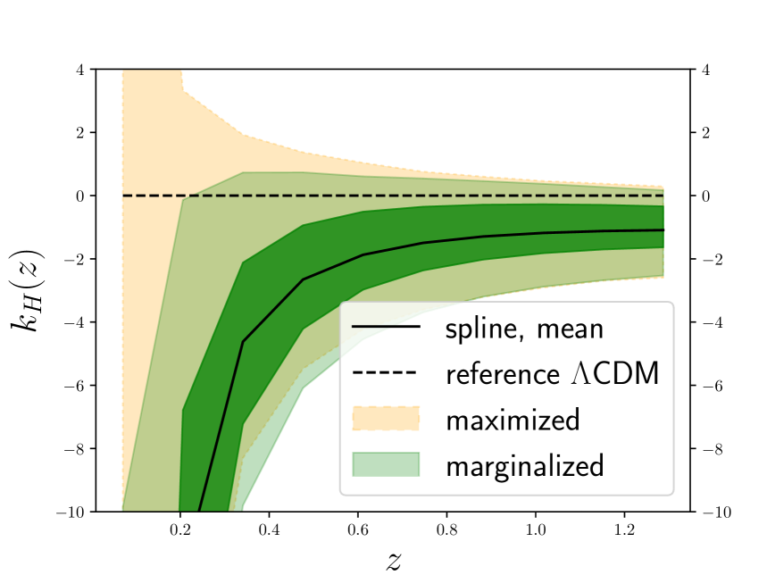
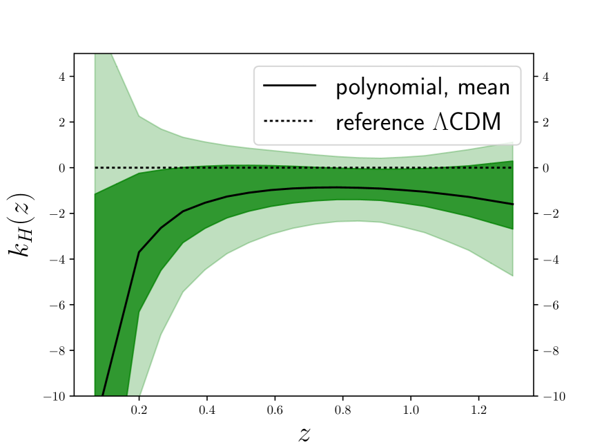
In figure 6 we show the consistency condition function obtained by fitting to the JLA+BC03+BAO data using both splines and polynomials. The polynomial fit shows no violation of the FRW consistency condition. In the spline case, there appears to be a significant deviation from , but this has to be treated with caution. As explained in section 5.2.1 (and discussed further in appendix section C), in the spline analysis we can have strong shifts in the 1-dimensional projected statistics due to the volume effect introduced by . The fact that the maximised contours (also plotted in in figure 6) do not show significant deviations from the FRW case is consistent with the interpretation that this is projection effect. When fitting JLA+MaStro+BAO data with splines, the marginalised 95% contours are consistent with . The large errors at low redshift are due to the fact that the denominator of goes to zero as when . The numerator diverges at least as rapidly, so the result is not divergent, but errors cause a mismatch between the measured values of the denominator and numerator. At large redshifts, in turn, the distance is less well determined. The best constraints over the redshift range are at for the polynomials and at for the splines. While polynomials are better constrained at intermediate redshifts, splines give smaller errors at large , reaching similar errors on as polynomials despite the fact that the distance is less well determined. This is not surprising since in the spline case we also fit the first derivative at the last spline knot , providing a better determination of in (2.1) than the polynomial case.
We also fit the polynomial to the JLA+BC03+BAO data assuming a constant . We use the FRW relation with a constant . The result is sensitive to the assumed value for , as found in [75]. Taking km/s/Mpc we get , whereas km/s/Mpc and km/s/Mpc give, respectively, and . (The results for the JLA+MaStro+BAO combination are similar, within the error bars.) For comparison, fitting the CDM model to the JLA data alone gives the (by construction constant) value . (The BC03+BAO data gives .) Taking into account the dependence on the parametrisation, on the debated value of and on the different stellar evolution models, the constraints can be conservatively summarised as . If the universe is well described by the FRW model, these numbers are a direct constraint on the spatial curvature parameter. A combination of the local value and the distance to the last scattering surface, which can be determined model-independently from the CMB [150, *Audren:2013nwa, 141], gives the constraint from the requirement that the universe is large enough to contain the last scattering surface [21].
These observational constraints on a constant are of the same order as the backreaction prediction shown in figure 2(e). However, in the case when is allowed to vary they loosen considerably; even at the best constrained redshift, for polynomials, our constraint on is about a factor of 3 weaker than the bound on a constant . Observational analyses where is taken to be constant therefore cannot be directly used as constraints on the magnitude of that varies with .
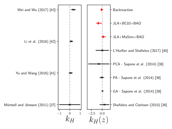
Our results roughly agree with those in the literature, with the caveat that the constraints depend on the dataset and the fitting method. Results for a constant are (95% C.I.) [69], (using a method applicable only for ) [73], [75] and [74]. Due to different model-dependence of the datasets and varying methods of fitting and determining the error bars, the strongest quoted constraints are not necessarily the most reliable. These limits are summarised in figure 7.
In figure 7 we also show results in the literature in the case when redshift dependence is taken into account. The results in the literature are [68], (with principal component analysis, PCA), (with Padé approximants, PA), (with genetic algorithms, GA) [70] and [72]. (The error bars from GA are very small, but they have been estimated with bootstrap methods [175].) These are limits for the redshifts for which the constraints are the tightest, determined by the balance between the low redshift mismatch divergence and poor accuracy of high redshift data. Apart from the case of genetic algorithms, the constraints loosen considerably. In [71, 72] it was also checked whether the data are consistent with the spatially flat FRW relation , but the error bars cannot be readily interpreted in terms of .
5.3 Forecast
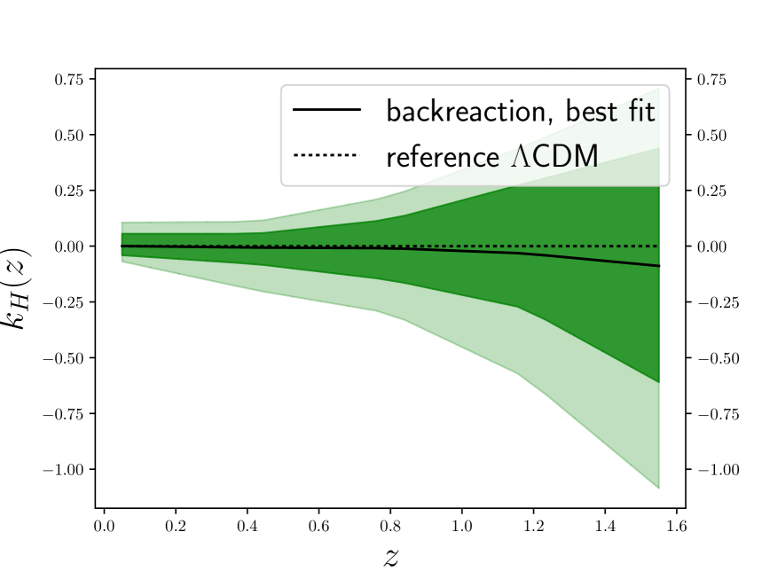
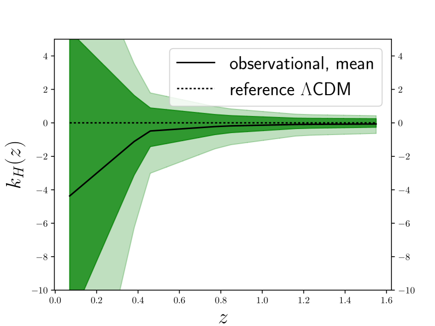
Finally, let us forecast how well next generation experiments can constrain .
We consider logarithmically spaced SNe Ia in the range . This is loosely modelled on a future catalogue combining observations from experiments such as LSST111111https://www.lsst.org/ and Euclid121212https://www.euclid-ec.org/ [176]. We assume fractional errors on the distance modulus equal to the mean of JLA fractional errors (the dispersion in the fractional error for different data points, about in JLA, is negligible for our purposes). We neglect nuisance parameters, as we only aim at a rough estimate. Given the larger redshift range spanned compared to JLA, fourth order polynomials do not recover the data well enough, so we model the luminosity distance with a fifth order polynomial.
Euclid [177] is also expected to measure differential ages of passive galaxies within the range . (See also [110, 178, 70] for discussion of future data.) We add the five simulated Hubble parameter datapoints from figure 2 of [105] to the BC03 data points listed in table 1. We consider the same second-order polynomial fit as before and marginalise over .
The data are rescaled to a fiducial flat CDM cosmology with and km/s/Mpc (we neglect realisation noise).
Given the different polynomial order of the SNIa fit, constraints on the distance coefficients cannot be readily compared to JLA results. However, the projected Hubble parameter results can be directly compared to those based on a BC03+BAO catalogue, rescaled at the fiducial cosmology. Error contours are similar, indicating that replacing the accurate BAO datapoints by the model-independent Euclid differential age datapoints will not degrade error bars even though the simulated Euclid errors on are about km/s/Mpc, contrasted with the BAO errors of km/s/Mpc.
On the left panel of figure 8 we show constraints on the consistency condition based on future SNIa data alone, calculating from the backreaction relation (2.7). As we assume the existence of a maximum in the angular diameter distance, we show the maximised (rather than marginalised) statistics, as before. Compared to figure 2(e), the forecasts show an improvement of a factor of 6 at low redshifts, with the tightest constraint at the minimum redshift having the 68% C.I. range and 95% C.I. range . Since in the forecast we keep nuisance parameters fixed, this improvement has to be interpreted as a lower possibly reachable bound on the errors. On larger redshifts the errors are comparable to present data. This indicates that, at large redshifts, the limiting systematic of this method is the bias introduced when determining (see section 4.5). Note that the upper limit of our projected SNIa data are close to the redshift of the angular diameter distance maximum in our fiducial model; the precision may vary depending on the real position of the maximum and reach of the SNIa data.
On the right panel of figure 8 we show the joint marginalised constraints on the consistency condition based on future SNIa and Hubble parameter data. Compared to figure 6, error contours decrease significantly, especially at large redshifts. The improvement is mainly driven by the larger number of SNIae. The tightest 68% C.I. limit is (the 95% C.I. limit is , reached at the largest redshift . This is a factor of 3 improvement compared to current data. This is comparable to the 68% C.I. limit obtained in [70] and based on a similar future SNIa catalogue as the one we have considered, but including Euclid BAO Hubble parameter data. Given that the expected magnitude from backreaction is [67], future observations are expected to probe the theoretically interesting region, but not cover it exhaustively.
6 Conclusions
We have fitted the JLA SNIa distance data with a fourth order polynomial, determined the expansion rate as a function of redshift using the backreaction relation (2.7) and calculated the resulting backreaction prediction for the FRW consistency functions , and . This method of determining the expansion rate requires the angular diameter distance to have a maximum. As the maximum is typically slightly outside the JLA data range (or is not clearly visible in the data), this means that many good fits have to be discarded. This selection effect leads to significant bias in marginalised parameters, but the maximised statistics give reliable results. The best fits for all three functions are approximately constant and equal to . The 95% C.I. range for and (which are essentially indistinguishable) varies between at small redshift and at , and is of the same order of magnitude.
We have also determined the function directly without cosmological assumptions (except for those associated with BAO data reduction) by combining the JLA SNIa distance data with cosmic clock and BAO expansion rate data. We have compared the results of fitting with polynomials or splines, and using either the BC03 or MaStro stellar population evolution models for cosmic clocks. We have carefully checked for bias and the reliability of the error bars with mock data and, in the case of splines, further guarded against overfitting with a cross-validation analysis. For splines we see a similar misleading volume effect as in the backreaction case, highlighting the importance of validating methods with mock data. The details show significant dependence on the stellar evolution model and the fitting method, but the overall trends are similar. At , errors are overwhelming due to the fact that is a ratio between two terms that vanish at and do not match precisely due to errors. The best 95% C.I. constraint, , is at for the polynomial fit (a similar constraint holds for splines) to the JLA+BC03+BAO data. Replacing BC03 data by MaStro data points gives at . In comparison, the constraints for a constant are nearly 3 times stronger, demonstrating that limits derived for a constant in the literature cannot be directly applied to backreaction, which (if significant) is expected to produce a with significant -variation. Furthermore, non-trivial redshift correlations and highly asymmetric error contours show the importance of consistently modelling the covariance matrix and the full non-Gaussian information, suggesting that care should be taken when using fitting methods such as Gaussian processes that rely on assumptions about correlations between different redshifts.
We have considered the value of determined from the data, and found that while the dependence on the fitting function is well within the 1 errors, the effect of the adopted stellar evolution model is larger, suggesting caution in the interpretation of these values, which are smaller than those determined from local SNe, although with large error bars.
Finally, we have done a forecast of the improvement expected from a future SNIa survey loosely modelled on LSST and Euclid and additional cosmic clock datapoints from Euclid galaxy differential age measurements. Observational constraints on tighten by up to a factor of 6 for the backreaction case and 3 for the model-independent case, reaching the order of magnitude where signatures of backreaction are expected if it is significant. However, a -dependent of this order of magnitude cannot be ruled out by next generation data of the kind we consider. The accuracy may be improved if the maximum of the angular diameter distances will be clearly determined by the data, which depends on a combination of redshift coverage and errors. Note also that our forecast is based on the spatially flat CDM model. The result may be different if the expansion rate or the distance has features, as is expected if backreaction is significant. This is difficult to take into account, as there is no reliable prediction for the change in the expansion rate due to backreaction, and the current data does not have strong constraining power for features. Nevertheless, we conclude that upcoming observations are expected to probe an interesting range of and that general model-independent tests such as the FRW consistency conditions continue to complement more precise model studies.
Acknowledgments
We thank Elisabetta Majerotto for contributing at an early stage of this work, and Martin Kunz and Jussi Väliviita for useful discussions.
Appendix A Roughness parameter for the spline fit
We do a cross-validation analysis in the spline case to avoid overfitting. Instead of computing the likelihood based directly on as in (4.3), we consider the following effective :
| (A.1) | |||||
where the constant is a roughness parameter. The first term is the introduced in (4.3). The explicit sum over the data points at redshifts highlights that in general they differ from the spline knots , where . The form of the penalty factor is inspired by smoothing spline algorithms [179, 180, 181]. The integral multiplying takes into account the mean curvature of the spline (the integrand is squared since we are not interested in the sign of the curvature). Values penalise irregularly oscillating functions that may fit noise (in the limit only linear functions would be allowed).
We select the optimal value of by demanding that if the underlying function is correctly recovered, it should accurately predict new independent data. This requirement is implemented by performing a -fold cross-validation (CV) [180, 181, 182]. First, we fix a value for and divide the data into two halves, and , homogeneously distributed in redshift (in practice, is given by the odd rows of a given catalogue and by the even rows). We then perform MCMC minimisation of on the first half that serves as a training dataset, determining the best fit spline parameters. The of the second half , which serves as a test dataset, is then computed at those best fit values, giving the score CVAB. If the training dataset is overfitted, the model so determined will predict poorly the test dataset, resulting in a large score CVAB. The roles of the two halves are switched and the procedure is repeated, determining the score CVBA. The total score CVAB+CVBA is stored for the parameter . The optimal value is the one that minimises CVAB+CVBA, reducing the risk of overfitting.
Given that at each step full MCMC chains are required, in practice we choose the optimal one among the five possibilities . The second derivatives appearing in (A.1) are computed as linear interpolations of the spline algorithm derivatives at the knot values. In our cubic spline algorithm we require second derivatives to be continuous and to vary linearly between two knots. Since we use second derivatives only to set the roughness parameters, the fact that they may be a poor approximation is not a concern.
The cross-validation analysis suggests that the selected number of spline knots does not overfit the supernova nor the Hubble parameter data, as they prefer the values and , respectively (and in the Hubble parameter case, the CV score of the case is very similar to the one for ).
Appendix B Redshift correlations
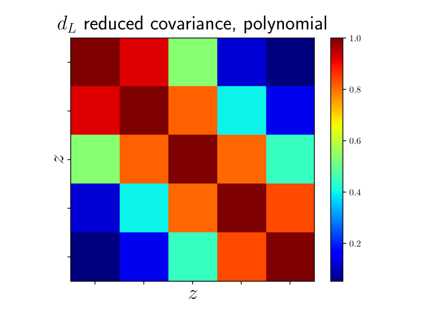
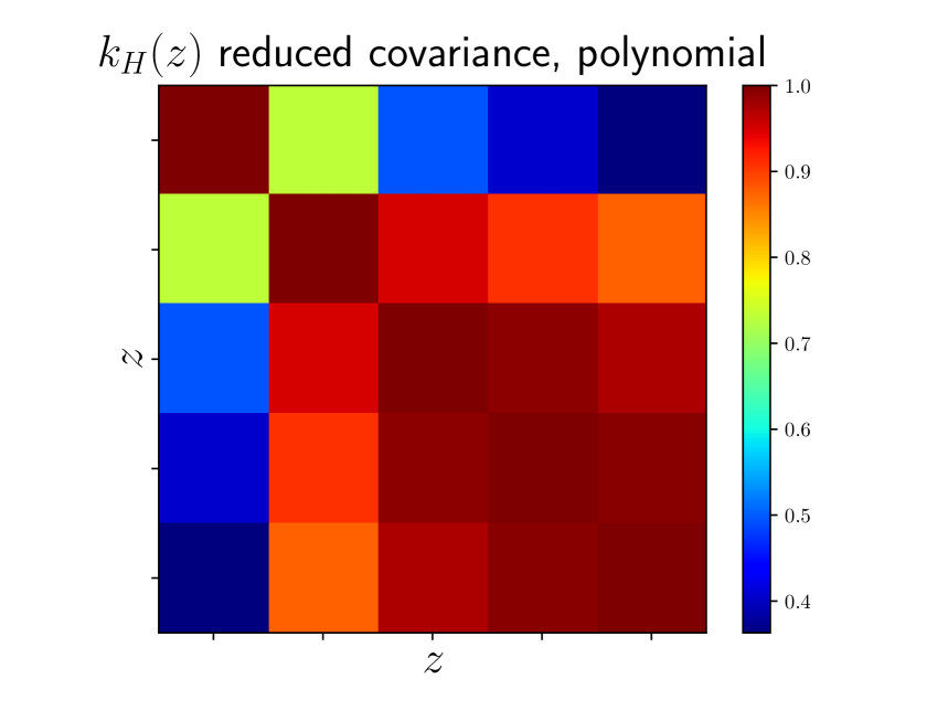
As discussed in section 4.4.4, our MCMC-based approach provides error contours on each function of redshift without restrictive assumptions about the underlying probability distribution. Furthermore, the covariance matrix computed from the chains provides information not only on the variance , but also on the correlations among the functions , at different redshifts , . To visualise to correlation between different redshifts we introduce the reduced correlation matrix
| (B.1) |
where is the matrix of the diagonal elements of a given covariance matrix .131313The elements of the reduced correlation matrix take values , and are equal to 1 on the diagonal by construction. If , no significant correlation is present between the corresponding -th and -th parameters (e.g. between the values of at redshifts and ).
Figure 9 shows the reduced correlation matrix for the luminosity distance and the consistency function for the polynomial fit to JLA data when is determined from the backreaction relation (2.7). In both cases there are important off-diagonal contributions. Redshift correlations are particularly significant for the consistency relation, partially because the Hubble parameter is obtained by integrating the distance over the redshift. While this correlates different redshifts non-trivially, the information is easily propagated through the MCMC algorithm. Besides these two examples, we have verified that all the functions considered in our analysis have important redshift correlations. The correlations in the CDM fit are similar as in the polynomial case, while in the spline case the off-diagonal terms are even larger.
Reconstruction techniques such as Gaussian processes rely on ansatzes about redshift correlations (see [138, 125] for discussion of the effects of different covariance functions). It is then important to model such non-trivial correlations correctly. Furthermore, as the strongly asymmetric error contours in the main text show, not all the functions can be well described by their second-order statistics alone and it is necessary to be able to model fully non-Gaussian profiles.
Appendix C Volume effect due to marginalisation
| Marginalised | ||
|---|---|---|
| Maximised |
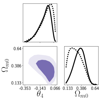
Figure 10 shows the marginalised posteriors for two of the parameters varied in the SN data fit when determining from (2.7) by demanding that is finite and real. The 1-dimensional plots show both the marginalised posteriors and the maximised profile likelihood. Table 3 shows the mean together with the 68% marginalised minimum credible intervals [183] (obtained by projecting all the points of the multi-dimensional parameter space onto 1-dimensional histograms) as well as the best fit together with the 68% confidence intervals (obtained by computing the maximum likelihood in each histogram bin).
Maximised confidence intervals describe the likelihood and are interpreted from a frequentist point of view, while the marginalised credible intervals are based on Bayesian posterior analysis. Maximised profiles have the advantage of preserving the true peak of the original multi-dimensional posterior probability. Marginalisation instead favours regions of parameter space that have large volume in the marginalised directions, and may lead to a misleading volume effect [183]. For example, consider the - plot in figure 10. It is instructive to compare the 2-dimensional posterior (keeping in mind it is obtained by projecting from a higher-dimensional space) to the 1-dimensional profiles for . While the global best fit is (given by the maximised profile, dashed line), there is a large amount of volume at higher values due to the large spread in the direction. This pushes the marginalised (projected) posterior mean to the larger value .
While the tension between the maximised and marginalised profiles is not severe when the error bars are taken into account, as we see from table 3, the differences are amplified in derived parameters such as , and hence in and .
References
- [1] C. J. Copi, D. Huterer, D. J. Schwarz and G. D. Starkman, Large angle anomalies in the CMB, Adv. Astron. 2010 (2010) 847541, [1004.5602].
- [2] Planck collaboration, P. A. R. Ade et al., Planck 2013 results. XXIII. Isotropy and statistics of the CMB, Astron. Astrophys. 571 (2014) A23, [1303.5083].
- [3] D. W. Hogg, D. J. Eisenstein, M. R. Blanton, N. A. Bahcall, J. Brinkmann, J. E. Gunn et al., Cosmic homogeneity demonstrated with luminous red galaxies, Astrophys. J. 624 (2005) 54–58, [astro-ph/0411197].
- [4] M. Scrimgeour et al., The WiggleZ Dark Energy Survey: the transition to large-scale cosmic homogeneity, Mon. Not. Roy. Astron. Soc. 425 (2012) 116–134, [1205.6812].
- [5] S. Nadathur, Seeing patterns in noise: Gigaparsec-scale ‘structures’ that do not violate homogeneity, Mon. Not. Roy. Astron. Soc. 434 (2013) 398–406, [1306.1700].
- [6] P. Laurent et al., A 14 Gpc3 study of cosmic homogeneity using BOSS DR12 quasar sample, JCAP 1611 (2016) 060, [1602.09010].
- [7] P. Ntelis et al., Exploring cosmic homogeneity with the BOSS DR12 galaxy sample, JCAP 1706 (2017) 019, [1702.02159].
- [8] F. S. Labini, Characterizing the large scale inhomogeneity of the galaxy distribution, AIP Conf. Proc. 1241 (2010) 981–990, [0910.3833].
- [9] F. S. Labini and L. Pietronero, The complex universe: recent observations and theoretical challenges, J. Stat. Mech. 1011 (2010) P11029, [1012.5624].
- [10] F. S. Labini, Inhomogeneities in the universe, Class. Quant. Grav. 28 (2011) 164003, [1103.5974].
- [11] F. S. Labini, Very large scale correlations in the galaxy distribution, EPL 96 (2011) 59001, [1110.4041].
- [12] C. Clarkson, B. Bassett and T. H.-C. Lu, A general test of the Copernican Principle, Phys. Rev. Lett. 101 (2008) 011301, [0712.3457].
- [13] R. Maartens, Is the Universe homogeneous?, Phil. Trans. Roy. Soc. Lond. A369 (2011) 5115–5137, [1104.1300].
- [14] W. B. Bonnor and G. F. R. Ellis, Observational homogeneity of the universe, Mon. Not. Roy. Astron. Soc. missing 218 (Feb., 1986) 605–614.
- [15] W. R. Stoeger, G. F. R. Ellis and C. Hellaby, The relationship between continuum homogeneity and statistical homogeneity in cosmology, Mon. Not. Roy. Astron. Soc. missing 226 (May, 1987) 373–381.
- [16] A. F. Heavens, R. Jimenez and R. Maartens, Testing homogeneity with the fossil record of galaxies, JCAP 1109 (2011) 035, [1107.5910].
- [17] C. Clarkson and R. Maartens, Inhomogeneity and the foundations of concordance cosmology, Class. Quant. Grav. 27 (2010) 124008, [1005.2165].
- [18] C. Clarkson, Establishing homogeneity of the universe in the shadow of dark energy, Comptes Rendus Physique 13 (2012) 682–718, [1204.5505].
- [19] T. Clifton, C. Clarkson and P. Bull, The isotropic blackbody CMB as evidence for a homogeneous universe, Phys. Rev. Lett. 109 (2012) 051303, [1111.3794].
- [20] S. Räsänen, A covariant treatment of cosmic parallax, JCAP 1403 (2014) 035, [1312.5738].
- [21] S. Räsänen, K. Bolejko and A. Finoguenov, New Test of the Friedmann-Lemaître-Robertson-Walker Metric Using the Distance Sum Rule, Phys. Rev. Lett. 115 (2015) 101301, [1412.4976].
- [22] M. F. Shirokov and I. Z. Fisher, Isotropic Space with Discrete Gravitational-Field Sources. On the Theory of a Nonhomogeneous Isotropic Universe, Soviet Astronomy missing 6 (Apr., 1963) 699.
- [23] T. Buchert and J. Ehlers, Averaging inhomogeneous Newtonian cosmologies, Astron. Astrophys. 320 (1997) 1–7, [astro-ph/9510056].
- [24] G. F. R. Ellis, Relativistic Cosmology: Its Nature, Aims and Problems, Fundam. Theor. Phys. 9 (1984) 215–288.
- [25] G. F. R. Ellis and W. Stoeger, The ’fitting problem’ in cosmology, Class. Quant. Grav. 4 (1987) 1697–1729.
- [26] G. F. R. Ellis and T. Buchert, The Universe seen at different scales, Phys. Lett. A347 (2005) 38–46, [gr-qc/0506106].
- [27] S. Rasanen, Backreaction: directions of progress, Class. Quant. Grav. 28 (2011) 164008, [1102.0408].
- [28] T. Buchert and S. Räsänen, Backreaction in late-time cosmology, Ann. Rev. Nucl. Part. Sci. 62 (2012) 57–79, [1112.5335].
- [29] T. Buchert, On average properties of inhomogeneous cosmologies, in Proceedings, 9th Workshop on General Relativity and Gravitation (JGRG9): Hiroshima, Japan, November 3-6, 1999, 1999. gr-qc/0001056.
- [30] C. Wetterich, Can structure formation influence the cosmological evolution?, Phys. Rev. D67 (2003) 043513, [astro-ph/0111166].
- [31] D. J. Schwarz, Accelerated expansion without dark energy, in 18th IAP Colloquium on the Nature of Dark Energy: Observational and Theoretical Results on the Accelerating Universe Paris, France, July 1-5, 2002, 2002. astro-ph/0209584.
- [32] S. Rasanen, Dark energy from backreaction, JCAP 0402 (2004) 003, [astro-ph/0311257].
- [33] S. Rasanen, Backreaction of linear perturbations and dark energy, in 39th Rencontres de Moriond Workshop on Exploring the Universe: Contents and Structures of the Universe La Thuile, Italy, March 28-April 4, 2004, 2004. astro-ph/0407317.
- [34] E. W. Kolb, S. Matarrese, A. Notari and A. Riotto, The Effect of inhomogeneities on the expansion rate of the universe, Phys. Rev. D71 (2005) 023524, [hep-ph/0409038].
- [35] S. R. Green and R. M. Wald, A new framework for analyzing the effects of small scale inhomogeneities in cosmology, Phys. Rev. D83 (2011) 084020, [1011.4920].
- [36] S. R. Green and R. M. Wald, Examples of backreaction of small scale inhomogeneities in cosmology, Phys. Rev. D87 (2013) 124037, [1304.2318].
- [37] S. R. Green and R. M. Wald, How well is our universe described by an FLRW model?, Class. Quant. Grav. 31 (2014) 234003, [1407.8084].
- [38] T. Buchert et al., Is there proof that backreaction of inhomogeneities is irrelevant in cosmology?, Class. Quant. Grav. 32 (2015) 215021, [1505.07800].
- [39] S. R. Green and R. M. Wald, Comments on Backreaction, 1506.06452.
- [40] J. J. Ostrowski and B. F. Roukema, On the Green and Wald formalism, in 14th Marcel Grossmann Meeting on Recent Developments in Theoretical and Experimental General Relativity, Astrophysics, and Relativistic Field Theories (MG14) Rome, Italy, July 12-18, 2015, 2015. 1512.02947.
- [41] S. R. Green and R. M. Wald, A simple, heuristic derivation of our ‘no backreaction’ results, Class. Quant. Grav. 33 (2016) 125027, [1601.06789].
- [42] J. Adamek, D. Daverio, R. Durrer and M. Kunz, General Relativistic -body simulations in the weak field limit, Phys. Rev. D88 (2013) 103527, [1308.6524].
- [43] J. Adamek, C. Clarkson, R. Durrer and M. Kunz, Does small scale structure significantly affect cosmological dynamics?, Phys. Rev. Lett. 114 (2015) 051302, [1408.2741].
- [44] J. Adamek, R. Durrer and M. Kunz, N-body methods for relativistic cosmology, Class. Quant. Grav. 31 (2014) 234006, [1408.3352].
- [45] J. Adamek, D. Daverio, R. Durrer and M. Kunz, General relativity and cosmic structure formation, Nature Phys. 12 (2016) 346–349, [1509.01699].
- [46] J. Adamek, D. Daverio, R. Durrer and M. Kunz, gevolution: a cosmological N-body code based on General Relativity, JCAP 1607 (2016) 053, [1604.06065].
- [47] C.-M. Yoo, H. Abe, K.-i. Nakao and Y. Takamori, Black Hole Universe: Construction and Analysis of Initial Data, Phys. Rev. D86 (2012) 044027, [1204.2411].
- [48] E. Bentivegna and M. Korzynski, Evolution of a periodic eight-black-hole lattice in numerical relativity, Class. Quant. Grav. 29 (2012) 165007, [1204.3568].
- [49] E. Bentivegna, Black-hole lattices, Springer Proc. Math. Stat. 60 (2014) 143–146, [1307.7673].
- [50] J. Adamek, M. Gosenca and S. Hotchkiss, Spherically Symmetric N-body Simulations with General Relativistic Dynamics, Phys. Rev. D93 (2016) 023526, [1509.01163].
- [51] E. Bentivegna, M. Korzyński, I. Hinder and D. Gerlicher, Light propagation through black-hole lattices, JCAP 1703 (2017) 014, [1611.09275].
- [52] J. T. Giblin, J. B. Mertens and G. D. Starkman, Departures from the Friedmann-Lemaitre-Robertston-Walker Cosmological Model in an Inhomogeneous Universe: A Numerical Examination, Phys. Rev. Lett. 116 (2016) 251301, [1511.01105].
- [53] J. B. Mertens, J. T. Giblin and G. D. Starkman, Integration of inhomogeneous cosmological spacetimes in the BSSN formalism, Phys. Rev. D93 (2016) 124059, [1511.01106].
- [54] E. Bentivegna and M. Bruni, Effects of nonlinear inhomogeneity on the cosmic expansion with numerical relativity, Phys. Rev. Lett. 116 (2016) 251302, [1511.05124].
- [55] J. T. Giblin, J. B. Mertens and G. D. Starkman, Observable Deviations from Homogeneity in an Inhomogeneous Universe, Astrophys. J. 833 (2016) 247, [1608.04403].
- [56] E. Bentivegna, An automatically generated code for relativistic inhomogeneous cosmologies, Phys. Rev. D95 (2017) 044046, [1610.05198].
- [57] H. J. Macpherson, P. D. Lasky and D. J. Price, Inhomogeneous Cosmology with Numerical Relativity, Phys. Rev. D95 (2017) 064028, [1611.05447].
- [58] J. T. Giblin, J. B. Mertens and G. D. Starkman, A cosmologically motivated reference formulation of numerical relativity, 1704.04307.
- [59] F. Ferrer and S. Rasanen, Dark energy and decompactification in string gas cosmology, JHEP 02 (2006) 016, [hep-th/0509225].
- [60] F. Ferrer, T. Multamaki and S. Rasanen, Fitting oscillating string gas cosmology to supernova data, JHEP 04 (2009) 006, [0812.4182].
- [61] F. Ferrer, Cosmological acceleration from a gas of strings, Nucl. Phys. Proc. Suppl. 194 (2009) 218–223, [0907.1342].
- [62] W. H. McCrea, Observable relations in relativistic cosmology. Mit 1 Abbildung., Zeitschrift fuer Astrophysik missing 9 (1935) 290.
- [63] S. Rasanen, Light propagation in statistically homogeneous and isotropic dust universes, JCAP 0902 (2009) 011, [0812.2872].
- [64] S. Rasanen, Light propagation in statistically homogeneous and isotropic universes with general matter content, JCAP 1003 (2010) 018, [0912.3370].
- [65] P. Bull and T. Clifton, Local and non-local measures of acceleration in cosmology, Phys. Rev. D85 (2012) 103512, [1203.4479].
- [66] M. Lavinto, S. Räsänen and S. J. Szybka, Average expansion rate and light propagation in a cosmological Tardis spacetime, JCAP 1312 (2013) 051, [1308.6731].
- [67] C. Boehm and S. Räsänen, Violation of the FRW consistency condition as a signature of backreaction, JCAP 1309 (2013) 003, [1305.7139].
- [68] A. Shafieloo and C. Clarkson, Model independent tests of the standard cosmological model, Phys. Rev. D81 (2010) 083537, [0911.4858].
- [69] E. Mortsell and J. Jonsson, A model independent measure of the large scale curvature of the Universe, 1102.4485.
- [70] D. Sapone, E. Majerotto and S. Nesseris, Curvature versus distances: Testing the FLRW cosmology, Phys. Rev. D90 (2014) 023012, [1402.2236].
- [71] R.-G. Cai, Z.-K. Guo and T. Yang, Null test of the cosmic curvature using and supernovae data, Phys. Rev. D93 (2016) 043517, [1509.06283].
- [72] B. L’Huillier and A. Shafieloo, Model-independent test of the FLRW metric, the flatness of the Universe, and non-local measurement of , JCAP 1701 (2017) 015, [1606.06832].
- [73] H. Yu and F. Y. Wang, New model-independent method to test the curvature of the universe, Astrophys. J. 828 (2016) 85, [1605.02483].
- [74] Z. Li, G.-J. Wang, K. Liao and Z.-H. Zhu, Model-independent estimations for the curvature from standard candles and clocks, Astrophys. J. 833 (2016) 240, [1611.00359].
- [75] J.-J. Wei and X.-F. Wu, An Improved Method to Measure the Cosmic Curvature, Astrophys. J. 838 (2017) 160, [1611.00904].
- [76] SDSS collaboration, M. Betoule et al., Improved cosmological constraints from a joint analysis of the SDSS-II and SNLS supernova samples, Astron. Astrophys. 568 (2014) A22, [1401.4064].
- [77] S. Rasanen, Light propagation and the average expansion rate in near-FRW universes, Phys. Rev. D85 (2012) 083528, [1107.1176].
- [78] S. M. Koksbang, Light propagation in Swiss cheese models of random close-packed Szekeres structures: Effects of anisotropy and comparisons with perturbative results, Phys. Rev. D95 (2017) 063532, [1703.03572].
- [79] I. M. H. Etherington, On the Definition of Distance in General Relativity., Philosophical Magazine 15 (1933) .
- [80] G. F. R. Ellis, Relativistic cosmology, Gen. Rel. Grav. 41 (2009) 581–660.
- [81] S. Rasanen, Cosmological acceleration from structure formation, Int. J. Mod. Phys. D15 (2006) 2141–2146, [astro-ph/0605632].
- [82] S. Rasanen, Accelerated expansion from structure formation, JCAP 0611 (2006) 003, [astro-ph/0607626].
- [83] K. Rosquist, Trigonometric parallaxes of distant objects - What they could tell about the universe, Astrophys. J. missing 331 (Aug., 1988) 648–652.
- [84] N. Suzuki et al., The Hubble Space Telescope Cluster Supernova Survey: V. Improving the Dark Energy Constraints Above z¿1 and Building an Early-Type-Hosted Supernova Sample, Astrophys. J. 746 (2012) 85, [1105.3470].
- [85] S. Nadathur and S. Sarkar, Reconciling the local void with the CMB, Phys. Rev. D83 (2011) 063506, [1012.3460].
- [86] SNLS collaboration, J. Guy et al., SALT2: Using distant supernovae to improve the use of Type Ia supernovae as distance indicators, Astron. Astrophys. 466 (2007) 11–21, [astro-ph/0701828].
- [87] G. R. Bengochea, Supernova light-curve fitters and Dark Energy, Phys. Lett. B696 (2011) 5–12, [1010.4014].
- [88] Z. Li, P. Wu and H. Yu, Probing the course of cosmic expansion with a combination of observational data, JCAP 1011 (2010) 031, [1011.2036].
- [89] M. C. March, R. Trotta, P. Berkes, G. D. Starkman and P. M. Vaudrevange, Improved constraints on cosmological parameters from SNIa data, Mon. Not. Roy. Astron. Soc. 418 (2011) 2308–2329, [1102.3237].
- [90] B. L. Lago, M. O. Calvao, S. E. Joras, R. R. R. Reis, I. Waga and R. Giostri, Type Ia supernova parameter estimation: a comparison of two approaches using current datasets, Astron. Astrophys. 541 (2012) A110, [1104.2874].
- [91] R. Giostri, M. V. dos Santos, I. Waga, R. R. R. Reis, M. O. Calvao and B. L. Lago, From cosmic deceleration to acceleration: new constraints from SN Ia and BAO/CMB, JCAP 1203 (2012) 027, [1203.3213].
- [92] R. Kessler et al., Testing Models of Intrinsic Brightness Variations in Type Ia Supernovae, and their Impact on Measuring Cosmological Parameters, Astrophys. J. 764 (2013) 48, [1209.2482].
- [93] J. T. Nielsen, A. Guffanti and S. Sarkar, Marginal evidence for cosmic acceleration from Type Ia supernovae, Sci. Rep. 6 (2016) 35596, [1506.01354].
- [94] H. Shariff, X. Jiao, R. Trotta and D. A. van Dyk, BAHAMAS: New Analysis of Type Ia Supernovae Reveals Inconsistencies with Standard Cosmology, Astrophys. J. 827 (2016) 1, [1510.05954].
- [95] D. Rubin and B. Hayden, Is the expansion of the universe accelerating? All signs point to yes, Astrophys. J. 833 (2016) L30, [1610.08972].
- [96] L. H. Dam, A. Heinesen and D. L. Wiltshire, Apparent cosmic acceleration from type Ia supernovae, Mon. Not. Roy. Astron. Soc. 472 (2017) 835–851, [1706.07236].
- [97] I. Tutusaus, B. Lamine, A. Dupays and A. Blanchard, Is cosmic acceleration proven by local cosmological probes?, Astron. Astrophys. 602 (2017) A73, [1706.05036].
- [98] SDSS collaboration, J. Marriner, J. P. Bernstein, R. Kessler, H. Lampeitl, R. Miquel, J. Mosher et al., A More General Model for the Intrinsic Scatter in Type Ia Supernova Distance Moduli, Astrophys. J. 740 (2011) 72, [1107.4631].
- [99] H. Campbell, M. Fraser and G. Gilmore, How SN Ia host-galaxy properties affect cosmological parameters, Mon. Not. Roy. Astron. Soc. 457 (2016) 3470–3491, [1602.02596].
- [100] C. Zhang, H. Zhang, S. Yuan, T.-J. Zhang and Y.-C. Sun, Four new observational data from luminous red galaxies in the Sloan Digital Sky Survey data release seven, Res. Astron. Astrophys. 14 (2014) 1221–1233, [1207.4541].
- [101] M. Moresco et al., Improved constraints on the expansion rate of the Universe up to z 1.1 from the spectroscopic evolution of cosmic chronometers, JCAP 1208 (2012) 006, [1201.3609].
- [102] BOSS collaboration, S. Alam et al., The clustering of galaxies in the completed SDSS-III Baryon Oscillation Spectroscopic Survey: cosmological analysis of the DR12 galaxy sample, Mon. Not. Roy. Astron. Soc. 470 (2017) 2617–2652, [1607.03155].
- [103] M. Moresco, L. Pozzetti, A. Cimatti, R. Jimenez, C. Maraston, L. Verde et al., A 6% measurement of the Hubble parameter at : direct evidence of the epoch of cosmic re-acceleration, JCAP 1605 (2016) 014, [1601.01701].
- [104] D. Stern, R. Jimenez, L. Verde, M. Kamionkowski and S. A. Stanford, Cosmic Chronometers: Constraining the Equation of State of Dark Energy. I: H(z) Measurements, JCAP 1002 (2010) 008, [0907.3149].
- [105] M. Moresco, Raising the bar: new constraints on the Hubble parameter with cosmic chronometers at , Mon. Not. Roy. Astron. Soc. 450 (2015) L16–L20, [1503.01116].
- [106] J. E. Bautista et al., Measurement of baryon acoustic oscillation correlations at with SDSS DR12 Ly-Forests, Astron. Astrophys. 603 (2017) A12, [1702.00176].
- [107] L. Verde, E. Bellini, C. Pigozzo, A. F. Heavens and R. Jimenez, Early Cosmology Constrained, JCAP 1704 (2017) 023, [1611.00376].
- [108] R. Jimenez and A. Loeb, Constraining cosmological parameters based on relative galaxy ages, Astrophys. J. 573 (2002) 37–42, [astro-ph/0106145].
- [109] D. P. Carson and R. C. Nichol, The age-redshift relation for Luminous Red Galaxies in the Sloan Digital Sky Survey, Mon. Not. Roy. Astron. Soc. 408 (2010) 213–233, [1006.2830].
- [110] T.-J. Zhang and C. Ma, Constraints on the Dark Side of the Universe and Observational Hubble Parameter Data, Adv. Astron. 2010 (2010) 184284, [1010.1307].
- [111] J. Simon, L. Verde and R. Jimenez, Constraints on the redshift dependence of the dark energy potential, Phys. Rev. D71 (2005) 123001, [astro-ph/0412269].
- [112] S. M. Crawford, A. L. Ratsimbazafy, C. M. Cress, E. A. Olivier, S.-L. Blyth and K. J. van der Heyden, Luminous Red Galaxies in Simulations: Cosmic Chronometers?, Mon. Not. Roy. Astron. Soc. 406 (2010) 2569, [1004.2378].
- [113] M. Moresco, R. Jimenez, A. Cimatti and L. Pozzetti, Constraining the expansion rate of the Universe using low-redshift ellipticals as cosmic chronometers, JCAP 1103 (2011) 045, [1010.0831].
- [114] A. Concas, L. Pozzetti, M. Moresco and A. Cimatti, On the robustness of the Lick index as a cosmic clock in passive early-type galaxies, Mon. Not. Roy. Astron. Soc. 468 (2017) 1747–1759, [1702.07348].
- [115] L. Verde, P. Protopapas and R. Jimenez, The expansion rate of the intermediate Universe in light of Planck, Phys. Dark Univ. 5-6 (2014) 307–314, [1403.2181].
- [116] G. Bruzual and S. Charlot, Stellar population synthesis at the resolution of 2003, Mon. Not. Roy. Astron. Soc. 344 (2003) 1000, [astro-ph/0309134].
- [117] C. Maraston and G. Stromback, Stellar population models at high spectral resolution, Mon. Not. Roy. Astron. Soc. 418 (2011) 2785, [1109.0543].
- [118] G. Efstathiou, H0 Revisited, Mon. Not. Roy. Astron. Soc. 440 (2014) 1138–1152, [1311.3461].
- [119] A. G. Riess et al., A 2.4% Determination of the Local Value of the Hubble Constant, Astrophys. J. 826 (2016) 56, [1604.01424].
- [120] W. Cardona, M. Kunz and V. Pettorino, Determining with Bayesian hyper-parameters, JCAP 1703 (2017) 056, [1611.06088].
- [121] B. R. Zhang, M. J. Childress, T. M. Davis, N. V. Karpenka, C. Lidman, B. P. Schmidt et al., A blinded determination of from low-redshift Type Ia supernovae, calibrated by Cepheid variables, 1706.07573.
- [122] B. Follin and L. Knox, Insensitivity of The Distance Ladder Hubble Constant Determination to Cepheid Calibration Modeling Choices, 1707.01175.
- [123] S. M. Feeney, D. J. Mortlock and N. Dalmasso, Clarifying the Hubble constant tension with a Bayesian hierarchical model of the local distance ladder, 1707.00007.
- [124] V. C. Busti, C. Clarkson and M. Seikel, Evidence for a Lower Value for from Cosmic Chronometers Data?, Mon. Not. Roy. Astron. Soc. 441 (2014) 11, [1402.5429].
- [125] V. C. Busti, C. Clarkson and M. Seikel, The Value of from Gaussian Processes, IAU Symp. 306 (2015) 25–27, [1407.5227].
- [126] C. Alcock and B. Paczynski, An evolution free test for non-zero cosmological constant, Nature 281 (1979) 358–359.
- [127] B. A. Bassett and R. Hlozek, Baryon Acoustic Oscillations, 0910.5224.
- [128] F. Montanari and R. Durrer, A new method for the Alcock-Paczynski test, Phys. Rev. D86 (2012) 063503, [1206.3545].
- [129] F. Lepori, E. Di Dio, M. Viel, C. Baccigalupi and R. Durrer, The Alcock Paczyński test with Baryon Acoustic Oscillations: systematic effects for future surveys, JCAP 1702 (2017) 020, [1606.03114].
- [130] E. Di Dio, Lensing smoothing of BAO wiggles, JCAP 1703 (2017) 016, [1609.09044].
- [131] X. Xu, A. J. Cuesta, N. Padmanabhan, D. J. Eisenstein and C. K. McBride, Measuring and H at from the SDSS DR7 LRGs using baryon acoustic oscillations, Mon. Not. Roy. Astron. Soc. 431 (2013) 2834, [1206.6732].
- [132] E. Gaztanaga, A. Cabre and L. Hui, Clustering of Luminous Red Galaxies IV: Baryon Acoustic Peak in the Line-of-Sight Direction and a Direct Measurement of H(z), Mon. Not. Roy. Astron. Soc. 399 (2009) 1663–1680, [0807.3551].
- [133] J. Miralda-Escude, Comment on the claimed radial BAO detection by Gaztanaga et al, 0901.1219.
- [134] F. S. Labini, N. L. Vasilyev, Y. V. Baryshev and M. Lopez-Corredoira, Absence of anti-correlations and of baryon acoustic oscillations in the galaxy correlation function from the Sloan Digital Sky Survey DR7, Astron. Astrophys. 505 (2009) 981–990, [0903.0950].
- [135] E. A. Kazin, M. R. Blanton, R. Scoccimarro, C. K. McBride and A. A. Berlind, Regarding the Line-of-Sight Baryonic Acoustic Feature in the Sloan Digital Sky Survey and Baryon Oscillation Spectroscopic Survey Luminous Red Galaxy Samples, Astrophys. J. 719 (2010) 1032–1044, [1004.2244].
- [136] A. Cabre and E. Gaztanaga, Have Baryonic Acoustic Oscillations in the galaxy distribution really been measured?, Mon. Not. Roy. Astron. Soc. 412 (2011) 98, [1011.2729].
- [137] M. Seikel, S. Yahya, R. Maartens and C. Clarkson, Using H(z) data as a probe of the concordance model, Phys. Rev. D86 (2012) 083001, [1205.3431].
- [138] M. Seikel and C. Clarkson, Optimising Gaussian processes for reconstructing dark energy dynamics from supernovae, 1311.6678.
- [139] J. E. Gonzalez, J. S. Alcaniz and J. C. Carvalho, Smoothing expansion rate data to reconstruct cosmological matter perturbations, JCAP 1708 (2017) 008, [1702.02923].
- [140] H. W. Chiang, A. E. Romano, F. Nugier and P. Chen, Probing homogeneity with standard candles, 1706.09734.
- [141] B. Audren, J. Lesgourgues, K. Benabed and S. Prunet, Conservative Constraints on Early Cosmology: an illustration of the Monte Python cosmological parameter inference code, JCAP 1302 (2013) 001, [1210.7183].
- [142] R. Trotta, Bayes in the sky: Bayesian inference and model selection in cosmology, Contemp. Phys. 49 (2008) 71–104, [0803.4089].
- [143] A. Gelman and D. B. Rubin, Inference from Iterative Simulation Using Multiple Sequences, Statist. Sci. 7 (1992) 457–472.
- [144] Planck collaboration, P. A. R. Ade et al., Planck intermediate results. XVI. Profile likelihoods for cosmological parameters, Astron. Astrophys. 566 (2014) A54, [1311.1657].
- [145] F. James and M. Roos, Minuit: A System for Function Minimization and Analysis of the Parameter Errors and Correlations, Comput. Phys. Commun. 10 (1975) 343–367.
- [146] C. Cattoen and M. Visser, Cosmography: Extracting the Hubble series from the supernova data, gr-qc/0703122.
- [147] M. Visser and C. Cattoen, Cosmographic analysis of dark energy, in Proceedings, 7th International Heidelberg Conference on Dark Matter in Astro and Particle Physics (DARK 2009): Christchurch, New Zealand, January 18-24, 2009, pp. 287–300, 2009. 0906.5407. DOI.
- [148] BOSS collaboration, T. Delubac et al., Baryon acoustic oscillations in the forest of BOSS DR11 quasars, Astron. Astrophys. 574 (2015) A59, [1404.1801].
- [149] P. Fleury, C. Clarkson and R. Maartens, How does the cosmic large-scale structure bias the Hubble diagram?, JCAP 1703 (2017) 062, [1612.03726].
- [150] M. Vonlanthen, S. Rasanen and R. Durrer, Model-independent cosmological constraints from the CMB, JCAP 1008 (2010) 023, [1003.0810].
- [151] B. Audren, Separate Constraints on Early and Late Cosmology, Mon. Not. Roy. Astron. Soc. 444 (2014) 827–832, [1312.5696].
- [152] J. Akeret, A. Refregier, A. Amara, S. Seehars and C. Hasner, Approximate Bayesian Computation for Forward Modeling in Cosmology, JCAP 1508 (2015) 043, [1504.07245].
- [153] J. L. Bernal, L. Verde and A. G. Riess, The trouble with , JCAP 1610 (2016) 019, [1607.05617].
- [154] C. Shapiro and M. S. Turner, What do we really know about cosmic acceleration?, Astrophys. J. 649 (2006) 563–569, [astro-ph/0512586].
- [155] Y. Gong and A. Wang, Observational constraints on the acceleration of the universe, Phys. Rev. D73 (2006) 083506, [astro-ph/0601453].
- [156] O. Elgaroy and T. Multamaki, Bayesian analysis of friedmannless cosmologies, JCAP 0609 (2006) 002, [astro-ph/0603053].
- [157] M. Seikel and D. J. Schwarz, How strong is the evidence for accelerated expansion?, JCAP 0802 (2008) 007, [0711.3180].
- [158] M. Seikel and D. J. Schwarz, Model- and calibration-independent test of cosmic acceleration, JCAP 0902 (2009) 024, [0810.4484].
- [159] E. Mortsell and C. Clarkson, Model independent constraints on the cosmological expansion rate, JCAP 0901 (2009) 044, [0811.0981].
- [160] A. C. C. Guimaraes, J. V. Cunha and J. A. S. Lima, Bayesian Analysis and Constraints on Kinematic Models from Union SNIa, JCAP 0910 (2009) 010, [0904.3550].
- [161] P. Serra, A. Cooray, D. E. Holz, A. Melchiorri, S. Pandolfi and D. Sarkar, No Evidence for Dark Energy Dynamics from a Global Analysis of Cosmological Data, Phys. Rev. D80 (2009) 121302, [0908.3186].
- [162] R.-G. Cai, Q. Su and H.-B. Zhang, Probing the dynamical behavior of dark energy, JCAP 1004 (2010) 012, [1001.2207].
- [163] S. Wang, X.-D. Li and M. Li, Exploring the Latest Union2 SNIa Dataset by Using Model-Independent Parametrization Methods, Phys. Rev. D83 (2011) 023010, [1009.5837].
- [164] J. Park, C.-G. Park and J.-c. Hwang, Analysis of recent type Ia supernova data based on evolving dark energy models, Phys. Rev. D84 (2011) 023506, [1011.1723].
- [165] A. V. Pan and U. Alam, Reconstructing Dark Energy : A Comparison of Cosmological Parameters, 1012.1591.
- [166] R.-G. Cai and Z.-L. Tuo, Detecting the cosmic acceleration with current data, Phys. Lett. B706 (2011) 116–122, [1105.1603].
- [167] X.-D. Li, S. Li, S. Wang, W.-S. Zhang, Q.-G. Huang and M. Li, Probing Cosmic Acceleration by Using the SNLS3 SNIa Dataset, JCAP 1107 (2011) 011, [1106.4116].
- [168] A. Shafieloo, A. G. Kim and E. V. Linder, Gaussian Process Cosmography, Phys. Rev. D85 (2012) 123530, [1204.2272].
- [169] A. Aviles, C. Gruber, O. Luongo and H. Quevedo, Cosmography and constraints on the equation of state of the Universe in various parametrizations, Phys. Rev. D86 (2012) 123516, [1204.2007].
- [170] J. Magaña, V. H. Cárdenas and V. Motta, Cosmic slowing down of acceleration for several dark energy parametrizations, JCAP 1410 (2014) 017, [1407.1632].
- [171] Q.-G. Huang and K. Wang, How the dark energy can reconcile Planck with local determination of the Hubble constant, Eur. Phys. J. C76 (2016) 506, [1606.05965].
- [172] Planck collaboration, P. A. R. Ade et al., Planck 2015 results. XIV. Dark energy and modified gravity, Astron. Astrophys. 594 (2016) A14, [1502.01590].
- [173] E. Aubourg et al., Cosmological implications of baryon acoustic oscillation measurements, Phys. Rev. D92 (2015) 123516, [1411.1074].
- [174] Planck collaboration, P. A. R. Ade et al., Planck 2015 results. XIII. Cosmological parameters, Astron. Astrophys. 594 (2016) A13, [1502.01589].
- [175] S. Nesseris and A. Shafieloo, A model independent null test on the cosmological constant, Mon. Not. Roy. Astron. Soc. 408 (2010) 1879–1885, [1004.0960].
- [176] P. Astier et al., Extending the supernova Hubble diagram to z 1.5 with the Euclid space mission, Astron. Astrophys. 572 (2014) A80, [1409.8562].
- [177] Euclid collaboration, R. Laureijs et al., Euclid Definition Study Report, 1110.3193.
- [178] J. C. Carvalho and J. S. Alcaniz, Cosmography and cosmic acceleration, Mon. Not. Roy. Astron. Soc. 418 (2011) 1873–1877, [1102.5319].
- [179] P. Green and B. Silverman, Nonparametric Regression and Generalized Linear Models: A roughness penalty approach. Chapman & Hall/CRC Monographs on Statistics & Applied Probability. Taylor & Francis, 1993.
- [180] C. Sealfon, L. Verde and R. Jimenez, Smoothing spline primordial power spectrum reconstruction, Phys. Rev. D72 (2005) 103520, [astro-ph/0506707].
- [181] H. V. Peiris and L. Verde, The Shape of the Primordial Power Spectrum: A Last Stand Before Planck, Phys. Rev. D81 (2010) 021302, [0912.0268].
- [182] F. Pedregosa et al., Scikit-learn: Machine Learning in Python, J. Machine Learning Res. 12 (2011) 2825–2830, [1201.0490].
- [183] J. Hamann, S. Hannestad, G. G. Raffelt and Y. Y. Y. Wong, Observational bounds on the cosmic radiation density, JCAP 0708 (2007) 021, [0705.0440].