The effect of nuclear gas distribution on the mass determination of supermassive black holes
Abstract
Supermassive black holes reside in the nuclei of most galaxies. Accurately determining their mass is key to understand how the population evolves over time and how the black holes relate to their host galaxies[1, 2, 3]. Beyond the local universe, the mass is commonly estimated assuming virialized motion of gas in the close vicinity to the active black holes, traced through broad emission lines[4, 5]. However, this procedure has uncertainties associated with the unknown distribution of the gas clouds. Here we show that the comparison of black hole masses derived from the properties of the central accretion disc with the virial mass estimate provides a correcting factor, for the virial mass estimations, that is inversely proportional to the observed width of the broad emission lines. Our results suggest that line-of-sight inclination of gas in a planar distribution can account for this effect. However, radiation pressure effects on the distribution of gas can also reproduce our findings. Regardless of the physical origin, our findings contribute to mitigate the uncertainties in current black hole mass estimations and, in turn, will help to further understand the evolution of distant supermassive black holes and their host galaxies.
Departamento de Astronomía, Universidad de Chile, Camino el Observatorio 1515, Santiago, Chile.
School of Physics and Astronomy, Tel Aviv University, Tel Aviv 69978, Israel.
Institute for Astronomy, Dept. of Physics, ETH Zurich, Wolfgang-Pauli-Strasse 27, CH-8093 Zurich, Switzerland.
Department of Physics, McGill University, Montreal, Quebec, H3A 2T8, Canada.
Active Supermassive black holes (SMBHs) are powered by accretion flows, probably in the form of accretion discs (ADs) that convert gravitational energy into radiation[6]. Gas in the Broad Line Region (BLR), located in the vicinity of the SMBH and moving at Keplerian velocities of thousands of kilometres per second, is photo-ionized by the AD producing broad emission lines. Under virial equilibrium, the observed width of these lines (in terms of full width at half maximum, ) can be used as a proxy for the virial velocity () and can be expressed as:
| (1) |
Here, is the gravitational constant, is the mean BLR distance to the SMBH and is the virial factor that accounts for the differences between the unknown and that are mostly caused by the BLR gas distribution of each object. Since even in the closest active galaxies the BLR cannot be resolved with current capabilities, is estimated from reverberation mapping (RM) experiments that show a strong correlation between the typical distance to the H emitting region and the continuum luminosity (the relation)[7, 8]. is assumed to be constant for all systems and is usually determined by requiring RM-based masses (from Equation 1) to agree, on average, with masses estimated from the relation between and the stellar velocity dispersion found in local galaxies[9, 10, 11]. This indirect technique to determine is known as the “single epoch virial method”[4, 5].
Unfortunately, the virial method is subject to biases and uncertainties associated with our ignorance of the dependence of on additional physical properties. These could include radiation pressure perturbations[12, 13], non virial velocity components[14, 15], the relative thickness () of the Keplerian BLR orbital plane[16], and the line-of-sight inclination angle ()[17, 18, 19] of this plane. An analytical expression for in the case of a planar BLR of thickness is given by:
| (2) |
where accounts for the line-of-sight projection of the Keplerian velocity of the BLR orbital plane[20, 21]. The nature of the velocity component responsible for the thickness of the BLR in unclear. However, ideas such as non-coplanar orbits, accretion disc radiation pressure, induced turbulence and outflowing disc winds have been suggested in the literature as plausible mechanisms to puff up the BLR[20, 22]. Given all these, the assumption of an universal introduces an uncertainty in the single epoch method which is estimated to be at least a factor of 2-3.
Recently, we used an alternative method to estimate by fitting the AD spectra of 37 active galaxies at z1.5 (about 1/3 of the current age of the universe), observed using the ESO X-Shooter spectrograph which provides simultaneous, very wide wavelength coverage of the AD emission[23, 24] (see supplementary information for sample description). The spectra were fitted with standard, geometrically thin, optically thick AD models[6] including general relativistic and disc atmosphere corrections[25]. In our modelling we made sure to avoid known model uncertainties that affect the short wavelength region (Å, see supplementary information). Each model is determined by several properties, mainly its (), the normalized accretion rate (expressed as the Eddington ratio ), the black hole spin () and the disc inclination to the line of sight (see supplementary information for model description). Crucially, this method only relies on our ability to model the AD. As a result, the derived masses are independent of the BLR geometry and kinematics, and therefore of any assumptions on the factor. For this sample, we also previously estimated the associated single epoch black hole masses () from the H, H, Mg ii and C iv broad emission lines[26]. As the relation has only been robustly established for the H line, the H, Mg iiand C iv single epoch masses are cross-calibrated to agree on average with the H mass estimations.
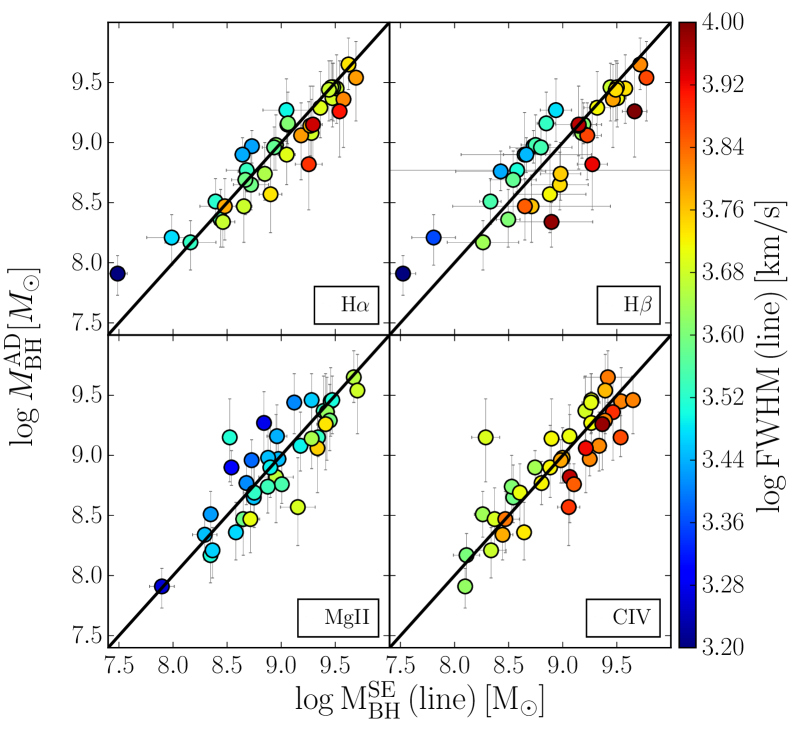
determinations from these two methods are compared in Figure 1. The approaches yield masses in very good agreement with each other (suggesting that AD and SE masses have comparable accuracies) albeit with significant scatter of a factor of about two[24]. In this letter we looked for possible drivers for this scatter and found a strong gradient in across the relation, as can be seen by the colour gradient of the data points in Figure 1.
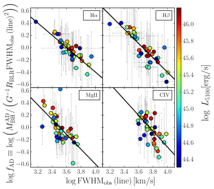
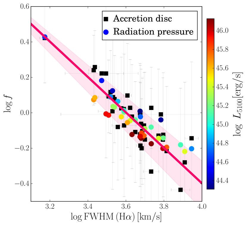
The ratio between and allows us to determine a proxy for the virial factor which we define as . In Figure 2 we show as a function of the for the H, H, Mg ii and C iv broad emission lines. Strong anti-correlations between and are present for all lines. These correlations are found to be significantly stronger than the expected correlations between and (see Table 1 and see supplementary information for details). We can conclude that the of the broad lines drives the discrepancies between and .
| (†) | (‡) | |||||
|---|---|---|---|---|---|---|
| Broad line | rs | Ps | rs | Ps | ||
| H | 4000700 | -1.000.10 | -0.85 | 4 | -0.44 | 5 |
| H | 45501000 | -1.170.11 | -0.84 | 8 | -0.48 | 2 |
| Mg ii | 3200800 | -1.210.24 | -0.75 | 9 | -0.23 | 2 |
| C iv | 56503000 | -1.290.35 | -0.61 | 6 | -0.25 | 1 |
We also determined how depends on and (see supplementary information). The dependence on is close to linear and, therefore, very different from the expected squared dependency found in Equation 1. The dependence on the monochromatic luminosities is consistent, within errors, with that found for single epoch calibrations (i.e., ). This indicates that has no impact on the scatter between and and that can be expressed as a single function of the of the broad emission lines. As can be seen in Table 1, our measurements are consistent within uncertainties with for all lines.
Previous works attempted to derive by comparing single epoch SMBH mass estimations with masses obtained from alternative methods. For instance, from the scaling relations between the black hole mass and the luminosity[27] or the stellar dispersion[18] of the host galaxy spheroidal components as well as from the amplitude of the excess X-ray variability variance that is found to be inversely anti-correlated with the black hole mass[28]. The results of these works also exhibit an anti-correlation between and the of the broad emission lines and were understood as an effect of line of sight inclination of the BLR. However, these works applies the same prescription to all systems, assuming that all objects are well represented by the median trend of the scaling relations, and do not take into account the large intrinsic scatter in such relations. This is in contrast with our sample where is independently obtained for each object through individual spectral fitting of the accretion disc emission.
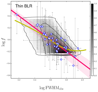
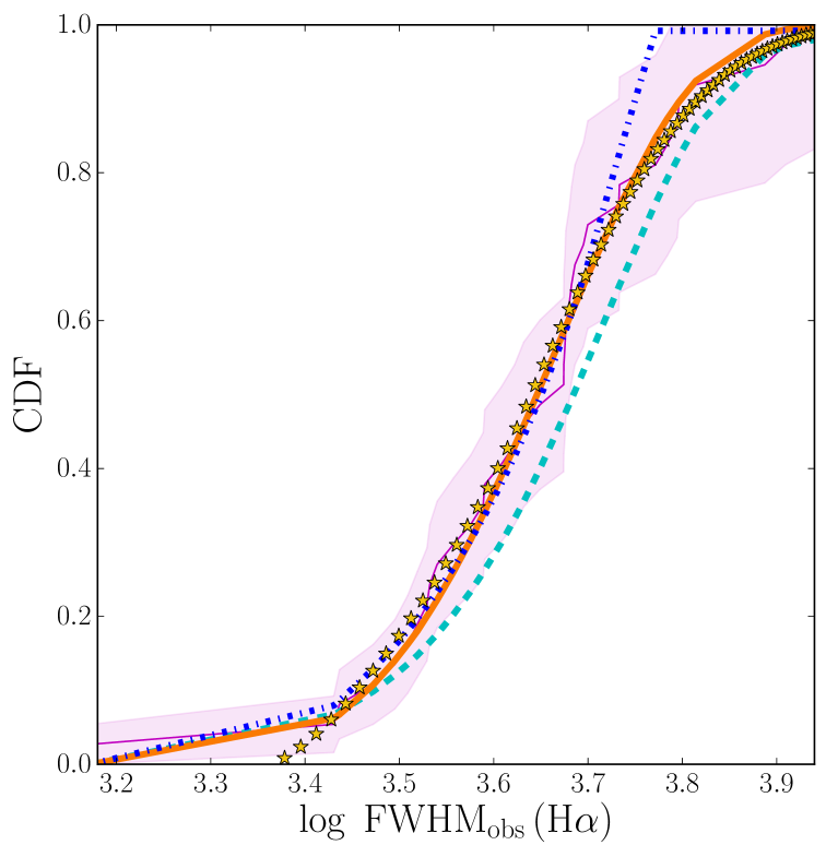
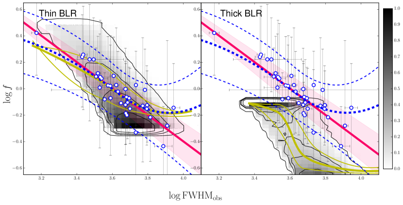
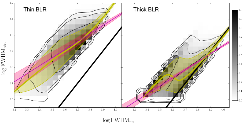
The high quality spectra in our sample and the careful modelling of its broad emission lines allow us to explore in detail whether the line of sight inclination in a disc-like BLR can reproduce the observed trends. For this purpose we prefer to use the data and correlations determined from the H line because of its high signal-to-noise ratio[26]. We define as the intrinsic full width at half maximum of the virialized velocity component of the BLR. To recover the virial expectation given by Equation 1 we use our result that for H (or equivalently FWHMobs) implying that, on average, . First, we adopt a model of a thin BLR (assuming that in Equation 2) and use Monte Carlo simulations to find the distribution that, after taking into account the line-of-sight inclination effects for randomly orientated BLRs, reproduces the cumulative distribution (see supplementary information for further details). Next, we generate a large population of objects drawn from the distribution and determine for each of these and FWHMobs. Finally, we compare the bi-dimensional –FWHMobs distribution obtained from our data with that generated from the simulations. We find that we are able to reproduce not only the mean trend of the observed correlation, but also the density distribution of data points, as can be seen in Figure 3. Furthermore, our simulations can recover the expected correlation (see extended data Figure E3). These results strongly indicate that line-of-sight inclination effects cause the observed –FWHMobs anti-correlation.
We also considered the combined effect of inclination and BLR thickness by assuming an universal within the range 0-1. We find that a wide range in thickness ratios () can reproduce the cumulative distribution function of , but only relatively thin BLRs () can reproduce the observed bi-dimensional distribution of and , and the predicted dependence.
We have also examined possible alternative scenarios. In particular, the effects of radiation pressure force in a gravitationally bound BLR can predict for some configurations[13]. This model predicts that the scatter in the relation will depend on the luminosity of the sources (see supplementary information). However, we do not find clear indications for this in our observations, as can be seen by the colour coded data points in Figure 2, where no clear gradient in is found across the –FWHMobs correlation. Note however that given the relatively narrow range in covered by our sample (a factor of 80), and the uncertainties in our estimations of , radiation pressure remains a intriguing mechanism that should be explored further in the future (see Extended data figure E4).
Regardless of its physical origin, the dependence of on implies that has been, on average, systematically overestimated for systems with large () and underestimated for systems with small (). The range of values presented in Figure 2, which are associated with 1600-8000 km s-1, imply a range in , and hence , of factor 6. However, this range should not be taken as representative of the entire population of AGN since our sample is too small (37 objects) and was not defined to be complete in terms of BLR properties.
Even though our sample is selected at a specific epoch (), the physics of a compact region such as the BLR is likely to remain constant over time. This has important implications for the study of active SMBHs at low and high redshifts. For example, the lowest sources at typically show relatively narrow BLR profiles (1000 km s-1 2000 km s-1). In this case, should be about 2-4 times larger than current estimates, and consequently should be smaller by the same factor. Another example is related to the mass of the most massive young known quasars found at . Our proposed dependence of with reduces the mass of the brightest known systems by up to a factor 2, as they typically show lines with 3000 km s-1, somewhat alleviating the tension between their outstandingly large masses and the very early epochs at which they have been discovered [29, 30]
References
- [1] Ferrarese, L. & Merritt, D. A Fundamental Relation between Supermassive Black Holes and Their Host Galaxies. ApJ 539, L9–L12 (2000). astro-ph/0006053.
- [2] Xiao, T. et al. Exploring the Low-mass End of the M BH-∗ Relation with Active Galaxies. ApJ 739, 28 (2011). 1106.6232.
- [3] Kormendy, J. & Ho, L. C. Coevolution (Or Not) of Supermassive Black Holes and Host Galaxies. ARA&A 51, 511–653 (2013). 1304.7762.
- [4] Trakhtenbrot, B. & Netzer, H. Black hole growth to z = 2 - I. Improved virial methods for measuring MBH and L/LEdd. MNRAS 427, 3081–3102 (2012). 1209.1096.
- [5] Shen, Y. The mass of quasars. Bulletin of the Astronomical Society of India 41, 61–115 (2013). 1302.2643.
- [6] Shakura, N. I. & Sunyaev, R. A. Black holes in binary systems. Observational appearance. A&A 24, 337–355 (1973).
- [7] Kaspi, S. et al. Reverberation Measurements for 17 Quasars and the Size-Mass-Luminosity Relations in Active Galactic Nuclei. ApJ 533, 631–649 (2000). astro-ph/9911476.
- [8] Bentz, M. C. et al. The Low-luminosity End of the Radius-Luminosity Relationship for Active Galactic Nuclei. ApJ 767, 149 (2013). 1303.1742.
- [9] Onken, C. A. et al. Supermassive Black Holes in Active Galactic Nuclei. II. Calibration of the Black Hole Mass-Velocity Dispersion Relationship for Active Galactic Nuclei. ApJ 615, 645–651 (2004). astro-ph/0407297.
- [10] Graham, A. W. Galaxy bulges and their massive black holes: a review. ArXiv e-prints (2015). 1501.02937.
- [11] Woo, J.-H., Yoon, Y., Park, S., Park, D. & Kim, S. C. The Black Hole Mass-Stellar Velocity Dispersion Relation of Narrow-line Seyfert 1 Galaxies. ApJ 801, 38 (2015). 1412.7225.
- [12] Marconi, A. et al. The Effect of Radiation Pressure on Virial Black Hole Mass Estimates and the Case of Narrow-Line Seyfert 1 Galaxies. ApJ 678, 693–700 (2008). 0802.2021.
- [13] Netzer, H. & Marziani, P. The Effect of Radiation Pressure on Emission-line Profiles and Black Hole Mass Determination in Active Galactic Nuclei. ApJ 724, 318–328 (2010). 1006.3553.
- [14] Denney, K. D. et al. Diverse Kinematic Signatures from Reverberation Mapping of the Broad-Line Region in AGNs. ApJ 704, L80–L84 (2009). 0908.0327.
- [15] Denney, K. D. et al. Reverberation Mapping Measurements of Black Hole Masses in Six Local Seyfert Galaxies. ApJ 721, 715–737 (2010). 1006.4160.
- [16] Gaskell, C. M. What broad emission lines tell us about how active galactic nuclei work. New Astronomy Review 53, 140–148 (2009). 0908.0386.
- [17] Wills, B. J. & Browne, I. W. A. Relativistic beaming and quasar emission lines. ApJ 302, 56–63 (1986).
- [18] Shen, Y. & Ho, L. C. The diversity of quasars unified by accretion and orientation. Nature 513, 210–213 (2014). 1409.2887.
- [19] Runnoe, J. C., Brotherton, M. S., DiPompeo, M. A. & Shang, Z. The behaviour of quasar C IV emission-line properties with orientation. MNRAS 438, 3263–3274 (2014). 1312.7500.
- [20] Collin, S., Kawaguchi, T., Peterson, B. M. & Vestergaard, M. Systematic effects in measurement of black hole masses by emission-line reverberation of active galactic nuclei: Eddington ratio and inclination. A&A 456, 75–90 (2006). astro-ph/0603460.
- [21] Decarli, R., Dotti, M., Fontana, M. & Haardt, F. Are the black hole masses in narrow-line Seyfert 1 galaxies actually small? MNRAS 386, L15–L19 (2008). 0801.4560.
- [22] Czerny, B., Du, P., Wang, J.-M. & Karas, V. A Test of the Formation Mechanism of the Broad Line Region in Active Galactic Nuclei. ApJ 832, 15 (2016). 1610.00420.
- [23] Capellupo, D. M., Netzer, H., Lira, P., Trakhtenbrot, B. & Mejía-Restrepo, J. Active galactic nuclei at z1.5 - I. Spectral energy distribution and accretion discs. MNRAS 446, 3427–3446 (2015). 1410.8137.
- [24] Capellupo, D. M., Netzer, H., Lira, P., Trakhtenbrot, B. & Mejía-Restrepo, J. Active galactic nuclei at z1.5 - III. Accretion discs and black hole spin. MNRAS 460, 212–226 (2016). 1604.05310.
- [25] Slone, O. & Netzer, H. The effects of disc winds on the spectrum and black hole growth rate of active galactic nuclei. MNRAS 426, 656–664 (2012). 1207.7074.
- [26] Mejía-Restrepo, J. E., Trakhtenbrot, B., Lira, P., Netzer, H. & Capellupo, D. M. Active galactic nuclei at z1.5 - II. Black hole mass estimation by means of broad emission lines. MNRAS 460, 187–211 (2016). 1603.03437.
- [27] Decarli, R., Labita, M., Treves, A. & Falomo, R. On the geometry of broad emission region in quasars. MNRAS 387, 1237–1247 (2008). 0804.1875.
- [28] Nikołajuk, M., Czerny, B., Ziółkowski, J. & Gierliński, M. Consistency of the black hole mass determination in AGN from the reverberation and the X-ray excess variance method. MNRAS 370, 1534–1540 (2006). astro-ph/0606621.
- [29] Mortlock, D. J. et al. A luminous quasar at a redshift of z = 7.085. Nature 474, 616–619 (2011). 1106.6088.
- [30] Wu, X.-B. et al. An ultraluminous quasar with a twelve-billion-solar-mass black hole at redshift 6.30. Nature 518, 512–515 (2015). 1502.07418.
- [31] McLure, R. J. & Dunlop, J. S. The black hole masses of Seyfert galaxies and quasars. MNRAS 327, 199–207 (2001). astro-ph/0009406.
- [32] Kaspi, S. et al. The Relationship between Luminosity and Broad-Line Region Size in Active Galactic Nuclei. ApJ 629, 61–71 (2005). astro-ph/0504484.
- [33] Bentz, M. C., Peterson, B. M., Netzer, H., Pogge, R. W. & Vestergaard, M. The Radius-Luminosity Relationship for Active Galactic Nuclei: The Effect of Host-Galaxy Starlight on Luminosity Measurements. II. The Full Sample of Reverberation-Mapped AGNs. ApJ 697, 160–181 (2009). 0812.2283.
- [34] Davis, S. W. & Laor, A. The Radiative Efficiency of Accretion Flows in Individual Active Galactic Nuclei. ApJ 728, 98 (2011). 1012.3213.
- [35] Netzer, H. & Trakhtenbrot, B. Bolometric luminosity black hole growth time and slim accretion discs in active galactic nuclei. MNRAS 438, 672–679 (2014). 1311.4215.
- [36] Peterson, B. M. & Wandel, A. Evidence for Supermassive Black Holes in Active Galactic Nuclei from Emission-Line Reverberation. ApJ 540, L13–L16 (2000). astro-ph/0007147.
- [37] Onken, C. A. & Peterson, B. M. The Mass of the Central Black Hole in the Seyfert Galaxy NGC 3783. ApJ 572, 746–752 (2002). astro-ph/0202382.
- [38] Done, C. & Krolik, J. H. Kinematics of the Broad Emission Line Region in NGC 5548. ApJ 463, 144 (1996). astro-ph/9510100.
- [39] Ulrich, M.-H. & Horne, K. A month in the life of NGC 4151: velocity-delay maps of the broad-line region. MNRAS 283, 748–758 (1996).
- [40] Sergeev, S. G., Pronik, V. I., Sergeeva, E. A. & Malkov, Y. F. Markarian 6 Nucleus since 1992. ApJS 121, 159–169 (1999).
- [41] Bentz, M. C. & Katz, S. The AGN Black Hole Mass Database. PASP 127, 67–73 (2015). 1411.2596.
- [42] Du, P. et al. Supermassive Black Holes with High Accretion Rates in Active Galactic Nuclei. IV. H Time Lags and Implications for Super-Eddington Accretion. ApJ 806, 22 (2015). 1504.01844.
- [43] Batiste, M., Bentz, M. C., Raimundo, S. I., Vestergaard, M. & Onken, C. A. Recalibration of the M BH- ⋆ Relation for AGN. ApJ 838, L10 (2017). 1612.02815.
- [44] Kollatschny, W. & Zetzl, M. Vertical broad-line region structure in nearby active galactic nuclei. A&A 558, A26 (2013). 1308.1902.
- [45] Kollatschny, W. & Zetzl, M. Broad-line active galactic nuclei rotate faster than narrow-line ones. Nature 470, 366–368 (2011).
- [46] Peterson, B. M. et al. Central Masses and Broad-Line Region Sizes of Active Galactic Nuclei. II. A Homogeneous Analysis of a Large Reverberation-Mapping Database. ApJ 613, 682–699 (2004). astro-ph/0407299.
- [47] Baron, D., Stern, J., Poznanski, D. & Netzer, H. Evidence that most type 1 AGN are reddened by dust in the host ISM. ArXiv e-prints (2016). 1603.06948.
- [48] Dunn, O. J. & Clark, V. Correlation Coefficients Measured on the Same Individuals. Journal of the American Statistical Association 64, 366–377 (1969).
- [49] Greene, J. E. & Ho, L. C. Estimating Black Hole Masses in Active Galaxies Using the H Emission Line. ApJ 630, 122–129 (2005). astro-ph/0508335.
- [50] McLure, R. J. & Dunlop, J. S. On the black hole-bulge mass relation in active and inactive galaxies. MNRAS 331, 795–804 (2002). astro-ph/0108417.
- [51] Laor, A., Barth, A. J., Ho, L. C. & Filippenko, A. V. Is the Broad-Line Region Clumped or Smooth? Constraints from the H Profile in NGC 4395, the Least Luminous Seyfert 1 Galaxy. ApJ 636, 83–89 (2006). astro-ph/0509200.
- [52] Pancoast, A. et al. Modelling reverberation mapping data - II. Dynamical modelling of the Lick AGN Monitoring Project 2008 data set. MNRAS 445, 3073–3091 (2014). 1311.6475.
- [53] Glen, A. G., Leemis, L. M. & Drew, J. H. Computing the distribution of the product of two continuous random variables. Computational Statistics & Data Analysis 44, 451–464 (2004).
- [54] Lopez, S. & Jenkins, J. S. The Effects of Viewing Angle on the Mass Distribution of Exoplanets. ApJ 756, 177 (2012). 1207.4477.
- [55] Foreman-Mackey, D., Hogg, D. W., Lang, D. & Goodman, J. emcee: The MCMC Hammer. PASP 125, 306–312 (2013). 1202.3665.
- [56] Ng, P. & Maechler, M. A fast and efficient implementation of qualitatively constrained quantile smoothing splines. Statistical Modelling 7, 315–328 (2007).
- [57] Afanasiev, V. L. & Popović, L. Č. Polarization in Lines - A New Method for Measuring Black Hole Masses in Active Galaxies. ApJ 800, L35 (2015). 1501.07730.
| E | F | vs | vs | ||||
|---|---|---|---|---|---|---|---|
| [1] | [2] | [3] | [4] | [5] | [6] | [7] | |
| 0.63 | 0.660.03 | 1.000.10 | 7.420.07 | 0.948 | 0.17 | 0.09 | |
| 0.65 | 0.690.04 | 0.820.11 | 7.430.09 | 0.943 | 0.24 | 0.12 | |
| MgII | 0.61 | 0.680.05 | 0.780.24 | 7.400.15 | 0.850 | 0.22 | 0.16 |
| CIV | 0.60 | 0.610.06 | 0.690.36 | 7.290.27 | 0.770 | 0.24 | 0.20 |
Supplementary Information
1 Sample description
The sample we use in this letter consists of 39 type-I AGN selected to be within a narrow redshift range around . For this sample we obtained high signal to noise () spectroscopic observations using the VLT/X-Shooter spectrograph. At the selected narrow redshift range, the X-Shooter spectrograph covers a wide range from 1200 Å to 9200 Å in the rest-frame. The sample was selected to homogeneously map the parameter space of and within the sampled region. The initial values of these quantities were obtained from single-epoch (SE) calibrations[4] of the H broad emission line and its adjacent continuum.
The broad spectral coverage and the high S/N in our sample allowed us to (1) re-calibrate, compare and test the performance of the different SE estimators using H, H, Mg ii and C iv[26]; and (2) model and confidently constrain the observed Spectral Energy Distributions (SEDs) in 37 out of 39 objects using standard thin accretion disc models[23, 24]. The output of the SED fitting provided alternative estimations for , , and a realistic estimate of . For the sake of simplicity, hereafter when referring to paper I, II and III we will be citing references 23, 26 and 24, respectively.
2 Estimating
In this section we briefly describe the two alternative approaches that we followed to derive and comment on the sources of uncertainties of each method.
2.1 Single Epoch estimates
We used the black hole masses obtained in paper II from the new calibrations of the single epoch (SE) black hole mass estimators for the broad , , and emission lines. In particular, we used the coefficients of the first two columns of Table 7 in Paper II. The underlying assumption in SE estimations is that Equation1 holds for all broad emission lines and can be estimated from the of the line in question using Equation 1. We used as suggested from -Stellar dispersion calibrations[11]. is obtained from the calibration of the relation obtained from various RM studies[7, 32, 33, 8] which can be written as:
| (3) |
where, is the normalization constant which for the case of the H line, and for Å, is 538 light-days[26].
As we briefly discussed in the letter, the simple SE mass determination method is limited in various important ways:
-
1.
The relation has been obtained from a relatively small sample of low-z () Seyfert I galaxies and low luminosity quasars (, where ). Therefore, extrapolation of the relation is needed to estimate in high luminosity objects at high-z. Moreover, the intrinsic scatter in the relation is affected by intrinsic luminosity variations as well as by the disc inclination to the line-of-sight[34, 35, 23].
-
2.
The re-calibration of the H-based single epoch method to other broad emission lines like H, Mg ii and C iv induces intrinsic dispersion that can be as high as 0.5 dex for the C iv line[26].
-
3.
The dependence of on inclination is a major source of uncertainty. This has been explored in numerous papers. A recent paper used a sample of about 600 local SDSS type1-AGN to compare the estimations derived from the -stellar dispersion relation () with those derived from the single epoch method[18]. They found that is anti-correlated with , and argued that this is a manifestation of the line-of-sight inclination in a flat, disc-like BLR. Earlier works also suggested an anti-correlation between the radio loudness of sources and the observed [17, 19]. Assuming that radio jets in AGN are aligned with the axis of symmetry of the BLR and that the flat BLR is aligned with the disc, their results strongly suggests that the BLR in radio-loud AGN are considerably flattened.
-
4.
There are questions regarding the validity of virial equilibrium of the BLR material. Earlier results about AGN with multiple emission measurements (i.e., NGC3783, NGC5548, NGC7469 and 3C390.3) show that the velocity radial profiles that are in good agreement with the expectations for a Keplerian system[36, 37] (i.e., ). Additionally, in some velocity resolved RM experiments, the blue wing of the H line has been observed to lag behind the red wing, which generally rules out significant outflow of both high- and low-ionization lines[38, 39, 40]. However, more recent RM observations revealed diverse kinematics of the BLR including inflows, outflows and virialized gas[14, 15].
-
5.
The use of a single value of for measuring in sources that are not part of RM samples introduces an additional uncertainty which results from the fact that the measured from single-epoch spectra are systematically larger than those measured from the RMS profiles during a RM campaign[20]. This can be easily verified by comparing the RMS [41] with the one measured from the mean spectrum of the same sources[42]. This is also true when the standard deviation of the lines () is used instead of the and has not been taken into account, properly, in many studies. For example, from the results published in a recent paper[43] we obtain .
-
6.
The line shape parameter provides information on the structure and kinematics of the BLR. For instance, is found for a spherical shell of clouds moving with fix a velocity and random orientations, is found for an face-on rotating ring with fixed velocity, corresponds to Gaussian profiles, is found for a face on rotating Keplerian disc, () corresponds to Lorentzian profiles due, for example, to turbulent motions, as well as logarithmic profiles which can be caused by in-/outflow motions, and corresponds to exponential profiles caused by electron scattering within the photo-ionized BLR gas[44]. is known to vary within a significant range[20, 45, 46] suggesting that BLR profiles are not universal and that the virial factor is far from being a constant value.
2.2 Black Hole Mass Estimates from SED fitting
As previously mentioned, in papers I and III we recently implemented an alternative method to estimate the black hole mass in type1-AGN based on the fitting of the SED of the accretion discs, using a geometrically thin, optically thick accretion disc model, and obtained successful fits in 37 out of 39 objects in our sample. The model is fully determined by , , , the AD inclination with respect to the line-of-sight (), and intrinsic . The procedure consisted of a Bayesian minimization over a grid of models covering a range in values for these parameters. We assumed Gaussian priors for and . Means were given by the single-epoch estimations for each object and standard deviations of 0.3 and 0.2 dex were adopted, respectively. and were calculated assuming a virial factor . Flat priors were assumed for the remaining model parameters. The role of the priors is to penalize models which deviate significantly from the observational estimations of and , but allow a symmetric parameter search on either side of the means. In the analysis presented in this letter we use the results obtained in paper III. To completely avoid complications in SED fittings resulting from unknown opacity and other effects in the disc atmosphere, for our Bayesian fitting we used only the X-shooter spectra with Å. At such wavelengths, our models are adequate and spectral features that may influence the spin parameter determination are not included in the fit.
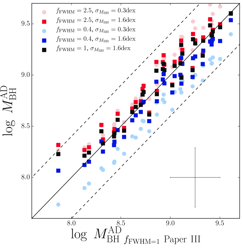
We have investigated the possibility that our initial choices of and the standard deviation in (), affect the resulting . As shown in Figure E5, this is not the case. In this Figure, we compare the resulting for a large range of initial guesses in and with the original values obtained for our sample in paper III (where and dex were assumed). We find that for large enough ( dex) there is basically no difference between the values obtained with our initial choices and those values obtained with an initial varying over a large range (0.4-2.5). Motivated on the previous findings, we re-ran our code using completely random mass priors within the interval of [8,10] and dex. We find that (1) the resulting “random-AD masses” do not show significant correlation with the assumed random priors (, ) and, crucially, that (2) random-AD masses are significantly correlated and consistent with SE masses from paper II with and . All these tests confirm the robustness of the BH mass measurements obtained by fitting AD SEDs as well as their comparable accuracy and good agreement and with SE mass measurements.
We also tested the reliability of the anti-correlation with found using our Bayesian algorithm. We explored whether the assumption of flat priors for and had an impact on our results. We tested various Gaussian priors on assuming as central values some randomly assigned numbers and different intrinsic scatters of 0.1, 0.2 and 0.3 dex. We also assumed Gaussian priors on . The central values were obtained from the recent calibrations of based on the ratio[47]. The intrinsic scatter were varied from 0.1 to 0.3 dex. In all cases we recover the anti-correlation between and the for the Balmer lines with similar statistical significance. We also used as the central value for the prior and tested using the median values, instead of the mean, for and . In both cases we recover the aforementioned anti-correlation with similar statistical significance. We conclude that our findings are not an artefact of the fitting code.
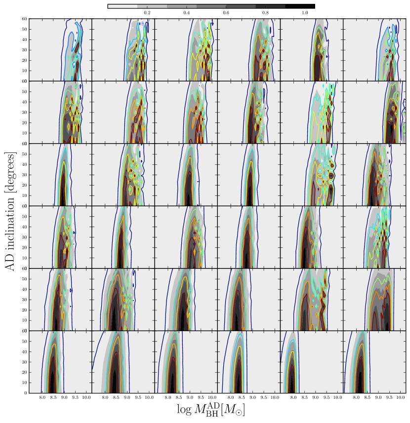
One important drawback from our modelling is a large degeneracy between the accretion rate and the inclination angle of the disc. For a given flux, larger inclinations will return larger intrinsic luminosities which in turn will return larger accretion rates. Fortunately, the derived black hole mass does not strongly depend on either inclination nor accretion rate and the mass estimates are consistent within 0.1 dex regardless of the final derived inclinations and accretion rates. This is confirmed in Figure E6 that shows the posterior bi-dimensional probability distribution of the accretion disk inclination versus in 36 out of 37 objects of our sample. Although the inclination is mostly unconstrained, the derived black hole mass is practically independent of the assumed inclination. As a consequence, the derived disc inclinations are very uncertain and are not good indicators of the real inclinations of the disc and consequently of the flat BLRs. Therefore, these values are not used as proxies for the inclination of the BLR and the determination of the virial factor.
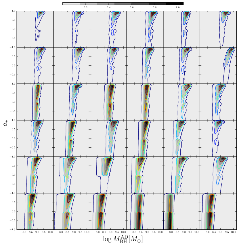
Finally, our results also show that the derived is mostly independent of . This is confirmed in Figure E7 that shows the posterior bi-dimensional probability distribution of versus in 36 out of 37 objects of our sample. It can be observed that although the spin is not tightly constrained, the black hole mass is restricted to a narrow range. This indicates that our AD mass determinations are not degenerated with . The reason for this is that the spin affects mostly the ionizing UV continuum emission while the mass depends mainly on the optical part of the AD spectrum.
3 as a function of line width
In Table 1 we present the correlation coefficients of the – and – correlations for all the broad emission lines considered here. In all cases we find that the correlations associated with the are stronger than those associated with . This suggests that the correlations are not inherited from the definition of . In order to prove this we conducted the Williams’s Test[48]. Given a sample size, this test computes the statistical significance of the difference between the correlation coefficients of two correlations that have one variable in common. In this case the two dependent correlations are – and –, while the common variable is . Our results indicate very different correlation coefficients for the – and the – correlations (see Table 1), with a 5- significance for the H line, 4- significance for the H and the Mg ii lines and a 3- significance for the C iv line. This confirms that the correlations associated with the of the broad emission lines are indeed much stronger than those that by definition are associated with .
Single epoch can also be estimated using instead of . Obviously, in that case the virial factor has a different numerical value since FWHM can be significantly different from (e.g., for a Gaussian line profile ). We tested whether the associated is also anti-correlated with and confirmed statically significant anti-correlations using all four emission lines. However, in this case there is no statistical difference between the – and – correlations. This is most likely due to the larger uncertainties associated with the measurement of in our sample[26].
To determine how depends on the of the lines and the associated used in single epoch mass determinations methods, we used the following expression:
| (4) |
and implemented an ordinary bi-variate least square linear regression to determine the coefficients in the equation. We summarize the results in Table E1, where we also show , which represents the slope of the power-law coefficient of in Equation 3. We also list the scatter between and as well as the scatter between and the corrected () after the dependency of on is taken into account. In the case of the Balmer lines, the scatter is reduced by about a factor 2. Thus, correcting for the correlation between and the of the Balmer lines provides an important improvement in our estimations.
The results of the linear regressions presented in Table E1 highlight two important findings. First, and are basically indistinguishable from each other. This indicates that has almost no impact in the deviation of from and that preserves its dependency on . Second, the dependence of on the observed of the Balmer lines is close to linear rather than quadratic, as expected from the virial relation.
4 Inclination as the source of the – correlation
In this section we present different tests that we carried out to determine whether inclination is driving the correlation between and .
Hereafter when referring to , and we mean , and the observed value of , unless otherwise specified. The reason to select the H line instead of the H line for the following analysis is the better S/N and hence more accurate measurements of in our sample. As shown in earlier works, in both Balmer lines are the same within uncertainties [49, 26].
The anti-correlation between and could be explained by the inclination of the axis of symmetry of a disc-like BLR with respect to the line-of-sight (LOS). If we consider the median LOS inclination, , at which Type-1 AGN are typically observed, we can also define a median virial factor at which the SE calibration represents an accurate black hole mass for objects observed at . Objects with narrower than usual broad emission lines are more likely observed at (face-on orientations) and objects with broader than usual emission are more likely observed at (edge-on orientations). This will produce too large (too small) SE mass estimates for objects with very broad (very narrow) emission lines, and would translate into a virial factor that anti-correlates with the line FWHMs.
The inclination hypothesis is also consistent with recent work that found that is anti-correlated with [18]. Here, is the black hole mass obtained from the correlation between and the stellar dispersion of the spheroidal component in galaxies. Analogously, an earlier work compared the virial black hole masses with black hole mass estimations obtained from the relation between black hole mass and the luminosity of the host-galaxy spheroidal component[27]. Their results also show a clear anti-correlation between and the of the broad emission lines that is interpreted by the authors as a BLR line-of-sight inclination bias.
There is further evidence that favours the hypothesis that LOS inclination is biasing SE estimations. As already pointed out, previous works found that the is significantly anti-correlated with radio core dominance in radio-loud quasars[17, 19]. This is consistent with H emitting gas in a flattened configuration. In this scenario core-dominated objects (with their radio emission being Doppler-boosted along the LOS) correspond to face-on discs that typically show narrow H profiles, while lobe-dominated objects (lacking Doppler-boosting) correspond to edge-on discs, that typically show broad H profiles. In this scenario, the BLR is flat and the general plane of motion is similar to the plane of rotation of the central disc. In addition to this, there is accumulated evidence in the literature favouring a disc-like geometry for the BLR[31, 50, 51, 21, 52].
For a disc-like BLR with a thickness ratio and inclination with respect to the line-of-sight we will have . Thus, for an ensemble of randomly orientated BLRs the final distribution of will depend on (1) the intrinsic distribution and (2) the range of possible random orientations at which the BLR can be observed, both of which are, a priori, not known.
To check the inclination hypothesis we first need to determine the distribution of that is consistent with the probability density distribution (PDF) of the observed . We then need to test whether it is possible to recover the anti-correlation of with and the linear dependence of on , as derived in this letter. In other words, we need to test whether a population of randomly generated inclinations and that satisfy the PDF of , can also account for:
| (5) |
and at the same time:
| (6) |
It is important to note that both predictions should be satisfied to guarantee inclination as the driving mechanism of the observed correlation between and . The reason for this is that each of these expressions tests the dependency between and the two independent distributions determined to reproduce : and . While Equation (5) tests the dependency between and (which is proportional to ), Equation (6) tests the dependency between and .
We first assumed a thin BLR by taking . We computed the PDF as the product of two independent random variables[53] and applied it to the special case where [54]. For the distribution, we assumed an underlying truncated normal distribution with certain mean (FWHMmean) and dispersion (FWHMstd). Our normal distribution was truncated to allow to vary between 1000 and 30000 km s-1. We also assumed that our sample is limited to objects with line-of-sight inclination angles between and , with determined by the torus opening angle. For an optimal exploration of the parameter space we ran a Monte Carlo Markov Chain simulation using the python code EMCEE[55]. For the simulation we used 20 independent walkers and 5000 iterations that mapped a total of models.
In the left panel of Figure E1 we compare the observed cumulative and its uncertainty (magenta thin line and shadowed region, respectively) with the predicted cumulative PDF from the model with the highest posterior probability (black line). The parameters of this model are: , , , , and . Our model successfully reproduces the observed cumulative PDF. However, a simple normal distribution (red dashed line) is also consistent with the data and cannot be rejected. We also determined the best fit model for a distribution with FWHM, i.e., effectively a single velocity. This model (dashed blue-line) is able to reproduce the distribution at low values of , but it is unable to account for the distribution at large velocity widths.
First, we tested whether our thin BLR model is successful in reproducing the – distribution seen in the data (i.e., Equation 5). In the left panel of Figure E3 we show the predicted bi-dimensional probability density distribution of the virial factor and the observed as predicted by the thin BLR model. The Figure includes contours showing 25%, 50%, 75% and 99% confidence limits contours (black-thin lines) centred around the maximum probability point. We also superposed the data from in Figure 2 (open-blue circles). The magenta line represents the derived relation . The thick yellow line is the median of the – distributions derived using a quantile non-parametric spline regression[56]. Analogously, the blue-dashed lines represent the 25%, 50% and 75% quantiles of the observational distribution. To obtained these quantiles, for each observed data we randomly generated 1000 points following the error distributions in and and then applied the COBS method to characterize the resulting distribution. We can notice that the median (50%-quantile) of the theoretical and observational distributions are in very good agreement. The scattered open-blue circles also show excellent agreement with the the bi-dimensional probability density function from the best model. Explicitly, we find that from our 37 objects, 21% fall inside the central 25% confidence level region, 51% fall inside the 50% confidence level region, 74% fall inside the 75% confidence level region, and 85% fall inside the 99% confidence level region.
Next, we tested for the same thin BLR model whether it is possible to recover the predicted relation between and (i.e., Equation 6). In the left panel of Figure E3 we show the predicted bi-dimensional probability distribution of versus using the model with the highest posterior probability. The magenta solid line and magenta shadowed region represent the expected relation and 1- uncertainties, respectively. The solid-yellow line and yellow shadowed region represent the median – and errors from the simulated bi-dimensional distribution. A good agreement is found between the simulations and the predicted relations. This implies that we are also able to recover the relation for the thin BLR model.
In order to test the effects introduced by a thick BLR (), we assumed a single for all objects and followed the same steps outlined for the case of a thin BLR. We found that a wide range in BLR thickness ratios () is able to reproduce the cumulative PDF. However, objects with large thickness ratios clearly fail to reproduce the bi-dimensional distributions of – and –, as can be seen in the right panels of Figures E2 and E3. We generally find that only relatively thin BLRs, i.e., those with , are able to reproduce both bi-dimensional distributions and the cumulative PDF. In particular, for a BLR with , we find that the derived values constrain the range of inclinations at which the BLR is observed in our sample to . This upper limit is consistent with typical expectations of a central torus hiding the BLR. We also find that the median virial factor in our sample, , corresponds to a median orientation of .
In summary, our results show that a population of randomly orientated, thin BLRs can successfully reproduce our observations. We can thus conclude that inclination is very likely the main reason for the observed – correlations.
5 Radiation pressure effects
We finally considered the possibility that non-virial BLR motions or winds induced by radiation pressure force might cause the observed - dependency. We first tested a simple model that assumes that the BLR is composed of homogeneous clouds that are optically thick to ionizing radiation but optically thin to electron scattering. The model predicts a dependency between the virial factor and the the normalized accretion rate, , of the form: , where is the true virial factor and depends on the fraction of ionizing radiation and the column density of the gas clouds that is assumed constant along the entire BLR[12]. From this expression we can see that underestimates the actual as increases. Equivalently, should increase as increases. However, we find no clear correlation between and in our data (, ), and therefore radiation pressure effects, as prescribed by this model, are not present in our objects. Note however that our sample is restricted to a relatively small range of (from to , corresponding to a variation by a factor of 30).
A more recent model considers the effects of radiation pressure in a more realistic BLR composed of pressure confined clouds, hence allowing the gas density of individual clouds to decrease with distance to the central black hole[13]. In this model the system is still bound by gravity and becomes smaller with increasing . The reason for this trend is that as increases, the clouds spend more time at large distances from the black hole, therefore increasing the median and decreasing the median BLR Keplerian velocities. To account for this effect, the authors of this model proposed a modified expression for :
| (7) |
where and are constants. The first term accounts for the observational relation described in Equation 3 and the second term represents a radiation pressure perturbation quantified by . When replaced into the virial mass equation (Equation 1) this relation leads to a simple quadratic equation on with solution:
| (8) |
or equivalently:
| (9) |
where rad and are the black hole mass and virial factor for a radiation pressure dominated BLR. , , and is a normalization constant. In the case when this would result in a close agreement with the inverse proportionality between and found in our data. Given that is found to be for all lines (Table E1), this would translate into an explicit dependency of on . We would then expect that the scatter in the – relation should be driven by . In Figure 2 larger (smaller) values of are represented by redder (bluer) colours. We can see that there is no clear suggestion that the scatter in driven by in any of the lines. Note however that the relatively narrow range in covered by our sample (from to ergs/s, corresponding to a factor of 80), together with the uncertainties in our estimations of , do not allow us to rule out this mechanism.
Testing this model further, we found the combination of parameters , and that best reproduce our measurements and the observed relation between and for the H line. To obtain dimensionless values for and we expressed , and FWHM in units of , and 1000 km s-1, respectively. Taking , as suggested by the observations (see Table E1), we carried out a Monte-Carlo Markov Chain exploration of the parameter space of the model and found that , and are able to reproduce our measurements with a scatter of 0.12 dex, preserving the experimental dependence of on as expressed in Equation 3 with a scatter of 0.05 dex. At the same time the results are able to reproduce the observed – relation with a scatter of 0.11 dex (see Figure E4, which presents our observations (black squares with error bars) together with the prescribed values for as given by Equation 9 (coloured circles without error bars)). However, we also found that the residuals between the predicted values and the best fit to the correlation are heavily correlated with (r, P), as can be seen by the colour gradient of our simulated points in the direction perpendicular to the correlation best fit in Figure E4. This bias is introduced by the explicit dependence of on which is not observed in our sample, although notice that the error bars of our derived values are of the order of, if not larger, than the expected dependence (see Figure E4). Finally, the dependency on vanishes when . For this case, however, we were unable to reproduce any the observables. Extending our sample towards lower luminosities should yield the final test to be able to confidently conclude whether this model can be the driving mechanism for the observed – correlation.
Further constraints to the models evaluated here may be provided by the new method to determine based on the spectropolarimetry of the broad lines[57]. This method takes advantage of the scattering in the dusty structure of the light coming from the BLR. The radial velocity gradient in the BLR induces a gradient in the position angle of polarization across the broad emission line profiles. The advantage of this method is that it provides estimations that are independent of the BLR inclination. Therefore, the application of this method will eventually allow us to differentiate between the effects of inclination and radiation pressure.