High-resolution reconstruction of cellular traction-force distributions: the role of physically motivated constraints and compressive regularization

I Abstract

We develop a method to reconstruct, from measured displacements of an underlying elastic substrate, the spatially dependent forces that cells or tissues impart on it. Given newly available high-resolution images of substrate displacements, it is desirable to be able to reconstruct small scale, compactly supported focal adhesions which are often localized and exist only within the footprint of a cell. In addition to the standard quadratic data mismatch terms that define least-squares fitting, we motivate a regularization term in the objective function that penalizes vectorial invariants of the reconstructed surface stress while preserving boundaries. We solve this inverse problem by providing a numerical method for setting up a discretized inverse problem that is solvable by standard convex optimization techniques. By minimizing the objective function subject to a number of important physically motivated constraints, we are able to efficiently reconstruct stress fields with localized structure from simulated and experimental substrate displacements. Our method incorporates the exact solution for the stress tensor accurate to first-order finite-differences and motivates the use of distance-based cut-offs for data inclusion and problem sparsification.

II Introduction

The adhesion of cells and tissues to their environment has profound consequences on processes such as cell polarization [1], division, differentiation [2], tissue morphology during development [3], wound healing [4, 5, 6], and cancer metastasis [7]. Hence, quantifying how cells attach to impart force on the surrounding material is an important technical challenge in cell biology.

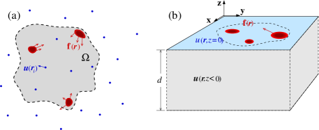
Cell motility and cellular response to signals have hitherto typically been studied in two-dimensional geometries in which cells are placed on a flat elastic substrate. Dynamic adhesion between the cells and the substrate are realized through dynamically reorganizing focal adhesions, often mediated through cellular structures such as lamellipodia and filopodia [8]. Focal adhesions are typically spatially localized, as shown in Fig. 1. Similarly, on larger length scales, a collection of cells can give rise to localized stress distributions. For example, the leading edge of a cell layer produces the pulling force that leads to migration in wound healing assays [4, 6, 5].

Figure 1: A schematic of an isolated cell. (a) The boundary of the cell footprint is denoted by the dashed curve, the support of the stress field is represented by the red regions that impart a stress ${\bf f}(x,y)$ on the surface. Displacements ${\bf u}({\bf r}_{i})$ of the elastic medium are measured at position ${\bf r}_{i}=x_{i}\hat{x}+y_{i}\hat{y}+z_{i}\hat{z}$ (blue dots) that can be inside or outside the cell footprint, on the surface ($z_{i}=0$), or below the surface ($z_{i}<0$). (b). A perspective view of the elastic substrate and cellular footprint.

Dynamically varying force-generating structures are often small and difficult to image. Mechanics-based methods for inferring their positions and magnitudes, such as using deformation of pillar structures [9] or textured substrates [10], have been developed. These methods require the cell to attach to a non-flat interface. The simplest method compatible with a flat interface relies on measuring the displacement of fiduciary markers, such as gold nanoparticles, embedded in the elastic substrate [11]. The measured displacements are an indirect probe of the force-generating structures, e.g., focal adhesions. Any inversion method should be able to not only reconstruct the positions and magnitudes of the stress field, but should ideally be able to capture potentially sharp boundaries of the stress-generating structures. However, fiduciary markers embedded in the 3D substrate are typically too sparse to reveal a displacement field with sufficient resolution to infer small cellular focal adhesion structures. To image such sub-cellular stress structures, high resolution reconstructions are required [12, 13]. Experimentally, new high-resolution imaging methods have been developed using methods to image higher densities of fiduciary markers [13] or fluorescent grid patterning of the substrate [14]. A surface grid pattern of fluorescent adhesion proteins allows surface deformation to be directly measured using conventional microscopes.

In light of such higher spatial resolution techniques, we develop an improved method for elastic stress source recovery using ideas developed for image segmentation [15]. This class of methods relies on optimization that uses “compressive” $L^{1}$ regularization terms in the objective function that favor solutions that are compactly supported [16, 17]. This type of regularization term is not derived from any fundamental physical law, but represents prior knowledge that the function to be recovered is sparse in content. In addition, the overall objective function will be constructed to obey physical constraints and symmetries.

In the next section, we review the standard linear equations of elasticity that describe the forward problem of computing the displacement field as a function of an arbitrary surface stress distribution. This model is then used to construct the data mismatch term in the objective function. We then motivate regularization and constraint terms in the full objective function. Finally, we demonstrate our method using both simulated and experimental data. Our method provides good reconstruction of localized structures that exhibit desirable qualities such compressive recovery of compact features as well as the suppression of Gibbs ringing phenomenon at the boundaries of the stress structures.

III Methods

III.1 Forward problem

We first derive the linear elastic Green’s function associated with a point force applied to the surface of a semi-infinite half-space, as shown in Fig. 1(b). We assume that the elastic medium is infinite in both depth ($d\to\infty$) and lateral extent. The Green’s function tensor defined in the domain ${\cal D}=\left\{(x,y,z)|x,y\in R,z\leq 0\right\}$ is given by

$${\bf G}=\left[\begin{matrix}G_{xx}(x,y,z)&G_{xy}(x,y,z)&G_{xz}(x,y,z)\\ G_{yx}(x,y,z)&G_{xy}(x,y,z)&G_{yz}(x,y,z)\\ G_{zx}(x,y,z)&G_{zy}(x,y,z)&G_{zz}(x,y,z)\end{matrix}\right]$$ (1)

where the components are explicitly given in Appendix A of the Supplementary Material. For example,

$$G_{sz,zs}(x,y,z)=\frac{1+\nu}{2\pi E}\left(\frac{sz}{R_{\perp}^{3}}\pm\frac{(1-2\nu)s}{R_{\perp}(R_{\perp}-z)}\right).$$ (2)

where $s\equiv x,y$. The equation with $\pm$ corresponds to $G_{sz}$ and $G_{zs}$, respectively, and $R_{\perp}\equiv\sqrt{x^{2}+y^{2}}$. The Young’s modulus and Poisson ratio of the elastic substrate are denoted by $E$ and $\nu$, respectively. For Matrigel, $E\approx 4\pm 3\times 10^{2}\textrm{ Pa}$ and $\nu\approx 0.5$ [18]. Throughout the rest of this manuscript, we will express stress in units of $E$. The displacement of a material point at $(x,y,z\leq 0)$ in the medium due to a stress distribution ${\bf f}$ is simply the convolution ${\bf u}({\bf r})\equiv[u_{x}\ u_{y}\ u_{z}]^{\intercal}={\bf G}\mathop{\scalebox{1.5}{\raisebox{-0.86108pt}{$\ast$}}}{\bf f}$.

For our specific problem, we shall restrict the forces to surface stresses ${\bf f}$ that act on the plane perpendicular to the $\hat{z}$ axis. We define the in-plane stress distribution, at depth $z$, as ${\bf f}(x,y)=f_{x}(x,y)\hat{x}+f_{y}(x,y)\hat{y}$. The resulting surface-level displacement fields become

$$u_{s}(x,y,z)=\sum_{k=x,y,z}\int_{\Omega}\mbox{d}x^{\prime}\mbox{d}y^{\prime}G_{sk}(x-x^{\prime},y-y^{\prime},z)f_{k}(x^{\prime},y^{\prime}).$$ (3)

Note that tangential stresses can induce displacements in the direction normal to the surface. For cells on flat surface, we assume that $f_{z}=0$.

III.2 Inverse problem

Next, we develop an objective function for which the minimizing solution provides a good approximation to the underlying stress field, while preserving discontinuities. The first component is simply a quadratic data mismatch term defined by the sum over the displacements measured at the $N$ measurement positions at ${\bf r}_{i}$:

$$\Phi_{\rm data}[{\bf f}]=\sum_{i}^{N}|{\bf u}^{\rm data}({\bf r}_{i})-{\bf u}({\bf r}_{i}|{\bf f})|^{2}.$$ (4)

Since ${\bf u}^{\rm data}({\bf r}_{i})$ is given, and ${\bf u}({\bf r}_{i}|{\bf f})$ is given by the linear model of Eq. 3, this contribution to the objective function is a functional over the surface force ${\bf f}(x,y)$. For simplicity, we will assume that the data points are measured only at the interface $z=0$ over an uniform grid with coordinates given $\{(x_{j},y_{k}):j\in\{1,2,\ldots,J\},k\in\{1,2,\ldots,K\}\}.$

In Eq. 3, we have restricted the domain of integration to lie within the cell footprint $\Omega$, reiterating that ${\bf f}(x,y)$ has compact support. As a consequence of compact support, for a fixed discretized approximation of ${\bf f}(x,y)$, the displacements can be obtained exactly by solving an equivalent system of linear equations of finite dimension. We explicitly define this system of linear equations given a piecewise-affine approximation of the stress field. Let us consider the first-order approximation of $f_{x}(x,y)$ and $f_{y}(x,y)$ using central finite differences, for $x\in[x_{j}-\delta x/2,x_{j}+\delta x/2)\cap y\in[y_{j}-\delta y/2,y_{j}+\delta y/2)$,

$$f_{x}(x,y)=f_{x}(x_{i},y_{j})$$

$$\qquad+(x-x_{i})\frac{f_{x}(x_{i+1},y_{j})-f_{x}(x_{i-1},y_{j})}{2\delta x}$$

$$\qquad+(y-y_{j})\frac{f_{x}(x_{i},y_{j+1})-f_{x}(x_{i},y_{j-1})}{2\delta y}$$

$$\qquad+\mathcal{O}(\delta x)^{2}+\mathcal{O}(\delta y)^{2},$$ (5)

where $i,j$ denotes a tuple of grid coordinates. In effect, we are performing sub-pixel interpolation where the stress is fully-determined by its values at the grid vertices.

Upon using Eq. 5, we can rewrite Eq. 3 by decomposing the integral into a sum of integrals over grid cells. After further regrouping terms, we find a linear system of equations for $u_{s}(x,y)$ across all grid points. For example,

$$u_{x}(x_{n},y_{m})=\Gamma_{xx}^{nmjk}f_{x}(x_{j},y_{k})+\Gamma_{xy}^{nmjk}f_{y}(x_{j},y_{k}),$$ (6)

where summation notation for each index tuple $(j,k)$ has been implicitly assumed, and the tensors $\Gamma_{xx}^{nmjk}$, $\Gamma_{xy}^{nmjk}$, and the analogous formulae for $u_{y}(x_{n},y_{m})$ are given in Appendix B of the Supplementary Material.

From an equation-counting perspective, the system of equations is exactly determined if and only if one has at least as many measurement points as grid cells in the resolution that one wishes to reconstruct the stress field, provided that one is able to measure displacements in both principle directions. Even if one is able to measure displacements in both directions, the measurements may be imprecise and noisy rendering the inversion of Eq. 6 highly ill-conditioned.  6 To resolve these issues, we introduce a number of physically consistent constraints and regularization terms relevant to this system.

III.3 Physical constraints and regularization

The remaining components of the objective function should contain information about the known physical constraints as well as regularization terms that better condition the overall optimization problem. Various regularization terms have been motivated, but they can also be associated with prior knowledge on the solution [19].

First, we consider explicit physical constraints. Since we are assuming inertial effects are negligible, we require that the net force vanish, or that

$$\int_{\Omega}f_{x}(x,y)\mbox{d}x\mbox{d}y=\int_{\Omega}f_{y}(x,y)\mbox{d}x\mbox{d}y=0.$$ (7)

Likewise, we require that there is no net torque, or that

$$\int_{\Omega}xf_{y}(x,y)\mbox{d}x\mbox{d}y=\int_{\Omega}yf_{x}(x,y)\mbox{d}x\mbox{d}y.$$ (8)

Similar no-force and no-torque constraints have been previously applied to the traction force inference problem in the Fourier domain [20] for which sparse solutions are difficult to resolve.

Another physical constraint is the requirement that surface stress at locations outside of the cell footprint vanish. In regions where there is no contact between the cell and the substrate, no mechanism can impart stress. Thus, the stress field is compactly supported within the cell footprint. The stress field may be further localized within cellular focal adhesions inside the cell footprint. Confining the stress to within an arbitrary cell footprint requires a complex iterative method [20].

To better condition the inference of ${\bf f}(x,y)$, we regularize this problem by forcing the reconstruction to obey some physically relevant characteristics of the surface stress. In many other types of inverse problems, for example, in the inference of the potential of mean force of a molecular bond, a constraint on differentiability is typically imposed on the function to be inferred [21]. A typical constraint of this nature may be a quadratic penalty on the gradients of the function to be inferred. However, such $L^{2}$ functional regularization often leads to over-smoothing of extreme values and failure to recover compactness. Thus, $L^{1}$ regularization on the function, or on its variations, have been developed to allow for more “compressed” reconstructions. These approaches are suitable for problems such as segmentation of images where boundaries are are sharp [16]. In these problems, the data is sparse in the sense that the boundaries in an image contain most of the information. Likewise, in the stress recovery problem at hand, the data consisting of displacements at a finite number of measurement positions may be considered sparse.

To this end one may employ variants of penalties often used in image processing applications, where one penalizes the $L^{1}$ norm of the vector field or its variations using regularization terms $\Phi_{\rm reg}$ of the form

$$\Phi_{L^{1}}=\int_{\Omega}\left(|f_{x}(x,y)|+|f_{y}(x,y)|\right){\bf d}{\bf r},$$ (9)

$$\Phi_{{\rm TV}_{1}}=\int_{\Omega}\left(|\nabla f_{x}(x,y)|+|\nabla f_{y}(x,y)|\right){\bf d}{\bf r}$$ (10)

and

$$\Phi_{{\rm TV}_{2}}=\int_{\Omega}\left(|\partial_{x}f_{x}|+|\partial_{y}f_{x}|+|\partial_{x}f_{y}|+|\partial_{y}f_{y}|\right){\bf d}{\bf r},$$ (11)

representing an $L^{1}$ regularization of the surface stress and two forms of its total variation, respectively. Since these regularization terms are not based on any fundamental physical law, there is some freedom in choosing their form. However, we do not want the choice of parameterization for the data grid to affect the reconstruction results. Hence, the regularization terms should not induce any additional anisotropy over that of the measured displacement field. Thus, appropriate regularizations should be invariant under coordinate rotation. Coordinate-invariant regularizers can be constructed from the magnitude of the force vector at the surface

$$|{\bf f}(x,y)|=\sqrt{f_{x}^{2}+f_{y}^{2}}.$$ (12)

Any regularization penalty imposed on the reconstruction problem must be a functional of this quantity in order to maintain rotational invariance relative to the choice of how the displacements are sampled. In this manuscript, we follow the approach taken by Han et al. [17] and focus on the isotropic $L^{1}$ norm

$$\tilde{\Phi}_{L^{1}}=\int_{\Omega}|{\bf f}(x,y)|\mbox{d}x\mbox{d}y.$$ (13)

Other regularizations are possible; for example, one may also use the isotropic $L^{2}$ norm

$$\tilde{\Phi}_{\rm L^{2}}=\int_{\Omega}|{\bf f}(x,y)|^{2}\mbox{d}x\mbox{d}y,$$ (14)

as was used by Plotnikov et al. [22].

Employing any of the above expressions as the regularization norm $\Phi_{\rm reg}$, we define the penalized optimization problem

$$\hat{{\bf f}}\big{|}\lambda=\arg\min_{{\bf f}}\left\{\Phi_{\textrm{data}}[{\bf f}]+\lambda\Phi_{\textrm{reg}}[{\bf f}]\right\},$$ (15)

subject to the no-force, no-torque, and footprint constraints (Eqs. 7 and 8) on ${\bf f}$ mentioned above. In Eq. 15, $\lambda>0$ is a tunable parameter. This problem is in a standard form that is directly solvable using a variety of optimization routines. In our implementation, we use a second-order quadratic cone solver [23].

To reduce the size of the system of equations described in Eqs. 6, we note that the Green’s function falls off at a rate of $|{\bf r}|^{-1}$. However, when combined with the zero-force constraint, the relationship between the displacements and the support of the stress field falls off at the much quicker rate of $|{\bf r}|^{-2}$ (see Appendix C in Supplementary Material). Formally, if $\Omega={\rm sup}({\boldsymbol{\sigma}})\subset\mathbb{R}^{2}$ is compact, and $\int{\boldsymbol{\sigma}}({\bf r}){\bf d}{\bf r}=\mathbf{0}$, then as $\mathbf{r}\to\infty$, $u_{x,y}({\bf r})=\mathcal{O}\left(|{\bf r}|^{-2}\right)$. The decay of the influence of stress on the system provides justification for setting distance-based cut-offs of the linear system. The effect of the cut-off is to limit the left-hand side of Eq. 6 to locations only within some maximal distance $R_{\perp}$ from the outline of the cell.

IV Results

We implemented our regularized inversion method in Python version 3.5, where optimization is performed using the cvxpy package with the ecos solver. Our implementation is available at https://github.com/joshchang/tractionforce. For all reconstructions, we assumed that $\nu=0.5$ and reported all results in normalized units of the Young’s modulus.

Figure 2: Test stress pattern and surface displacements. (a) Four focal adhesions attached by filaments indicated by the green lines. The red border represents the extent of the cell footprint and can be determined experimentally as part of the imaging. Mathematically, the cell boundary forms the basis for a constraint on the stress distribution and we explore the dependence of the quality of reconstruction on the footprint constraint. The faint blue grid represents the regular points at which displacements might be measured. (b) and (c) show, schematically, the corresponding surface displacements $u_{x}(x,y)$ and $u_{y}(x,y)$, respectively.

IV.1 Simulated data

First, we tested our method on simulated data derived from a force- and torque-free test stress field shown in Fig. 2. The test pattern consists of four separated circular stress pads, or focal adhesions, with radii $r_{1}=1/5$, $r_{2}=1/6$, $r_{3}=1/8$, and $r_{4}=1/4$, and centers at positions $(x_{1},y_{1})=(-1,-1/2)$, $(x_{2},y_{2})=(0,-1)$, $(x_{3},y_{3})=(2,1)$, and $(x_{4},y_{4})=(0,1)$. The pads 2,3, and 4 are connected in a triangle as shown, while pad 1 is connected only to pad 2. The tensions along these connections give rise to surface stresses imparted by the pads onto the substrate. We will assume that the stress fields in pads 1,2, and 3 are uniformly distributed within the circular disks. For pad 4, we assume that the filaments connected to it are distributed according to a cone-like density function. Thus, the stress field within pad 4 linearly decrease along the radial direction. The stresses ${\bf f}^{(i)}$ under each patch $i$ are decomposed into contributions arising from the total tension $T_{ij}$ connecting them with pad $j$ and can be expressed in the form

$${\bf f}^{(1)} =a_{12}\left(\hat{x}-{\hat{y}\over 2}\right)$$ (16)

$${\bf f}^{(2)} ={G_{4}\over A_{2}}\hat{y}-a_{12}{A_{1}\over A_{2}}\left(\hat{x}-{\hat{y}\over 2}\right)+a_{23}(\hat{x}+\hat{y})$$ (17)

$${\bf f}^{(3)} =-\hat{x}{G_{4}\over A_{3}}-a_{23}{A_{2}\over A_{3}}(\hat{x}+\hat{y})$$ (18)

$${\bf f}^{(4)} =g_{4}\left(1-{r\over r_{4}}\right)(\hat{x}-\hat{y})$$ (19)

where $a_{12},a_{23},g_{4}>0$ are constant amplitudes, $A_{i}=\pi r_{i}^{2}$ are the pad areas, and

$$G_{4}=2\pi g_{4}\int_{0}^{r_{4}}\left(1-{r\over r_{4}}\right)r\mbox{d}r={g_{4}\pi r_{4}^{2}\over 3}$$ (20)

is the total force on pad 4 in each direction. Note that both test stress fields are constructed to be force- and torque-free.

Figure 3: Comparing different regularizers. Reconstruction of the test patterns using all constraints and the different forms of $\Phi_{\rm reg}$: $\Phi_{L^{1}},\Phi_{{\rm TV}_{1}},\Phi_{{\rm TV}_{2}}$,$\tilde{\Phi}_{L^{1}}$ and $\tilde{\Phi}_{\rm{L}_{2}}$. Regularization parameters chosen according to Fig. D1 in Appendix D of the Supplementary Material.

In our examples, we used $a_{12}=10^{-4}$, $a_{23}=2\times 10^{-4}$, and $g_{4}=9\times 10^{-5}$. We generated displacement fields by solving the forward problem of (i.e., Eq. 3 for surface values ${\bf u}(x,y,z=0)$) and then corrupted the displacements with Gaussian white noise with standard deviation $10^{-5}$. From these noisy displacements, we reconstructed $f({\bf r})$.

Figure 4: Grid coarsening. Using every $n\in\{1,2,4\}$ lattice points of observations. The reconstruction is also performed at the same resolution. In general, the optimization is stable and the qualitative features of the reconstructed ${\bf f}(x,y)$ are robust to modest data coarsening.

Fig. 3 compares the reconstruction achieved from using the different forms of $\Phi_{\rm reg}$. In all of these reconstructions, we have imposed that the surface stress is both force-free and torque-free, and also that the support of the surface stress is within given the boundary defined in Fig. 2. The adjustable parameter $\lambda$ was chosen in each instance by examining the balance between data mismatch and regularity using trade-off curves shown in Fig. D1 in Appendix D, and taking the value for $\lambda$ that yields a point farthest away from the line segment joining the ends of the plot. The chosen value of $\lambda$ corresponds to a balance between regularity and data fidelity. The solution corresponding to each particular value of $\lambda$ is shown in Fig. 3. Each column in Fig. 3 corresponds to the use of a different regularization penalty. The parameter $\lambda$ can also be extracted using a Bayesian framework in which posterior probability is maximized [22].

Fig. 3 indicates that all forms of regularization yield reasonable reconstructions of the four pads, albeit at different levels of scarcity in reconstruction of the surrounding regions. The reconstruction using the isotropic $L^{1}$ penalty is seen to be more sparse than that of the isotropic $L^{2}$ penalty, whereas the other penalties all yielded comparable reconstructions. In the remaining analysis of the 4-pad test pattern we concentrate on using $\tilde{\Phi}_{L^{1}}$.

Figure 5: Unidirectional displacement measurements. We explore surface stress reconstruction from displacements only in one direction. Reconstructions of both components of the four-pad surface stress shown under measures along only $\hat{x}$ or only $\hat{y},$ using the $\tilde{\Phi}_{L^{1}}$ norm.

In many inverse problems, computational complexity is a technical issue either due to memory constraints or computational time. A tactic for reducing computational complexity is to coarsen the reconstruction problem so that one reduces the rank of the linear system to solve. Fig. 4 shows reconstructions of the 4-pad test patterns using $\tilde{\Phi}_{L^{1}}$ as a function of the coarseness of the displacement data. We coarsened the data by taking only every $n\in\{1,2,4\}$ lattice points in each dimension, noting that doing so reduces the rank of the problem by a factor of $n^{2}$. The general features of the stress patterns are preserved under coarsening but sufficient density of data points are needed to resolve fine scale variations in the stress field.

Figure 6: Constraints are unsatisfied unless enforced. Plotted are best reconstructions under $\tilde{\Phi}_{L^{1}}$ penalty and the difference between these reconstructions and the corresponding fully constrained reconstruction in Fig. 3.

Figure 7: Footprint misspecification. Reconstructions performed with the footprint drawn in an incorrect orientation. The erroneous footprint constraint misses two of the stress pads, resulting in a erroneous forces distributed along the edge of the footprint. If the misspecified footprint misses actual stress pads, spurious stresses will be generated at the misspecified boundaries in order to satisfy the no-force and no-torque constraint.

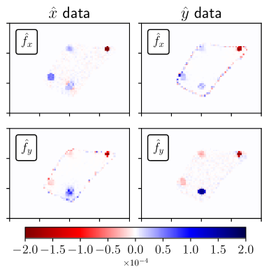
In some applications, displacements are only measurable along a single axis. Reconstruction of the surface forces using this type of data is related to the problem of missing data or information loss. We tested reconstruction under these circumstances by assuming that displacements only in either the $\hat{x}$ or the $\hat{y}$ directions are measured. In Fig. 5 we show reconstructions using only $u_{x}$ or $u_{y}$ data. In both cases, the reconstruction of the force in the direction perpendicular to the measured displacements is most affected by information loss. This effect is seen in the spurious boundary forces generated at the cell boundary in both cases. Nonetheless, the pads are clearly visible in both sets of reconstructions, along both axes.

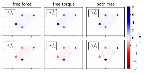
In all reconstructions so far, we have enforced the physical no-force and no-torque constraints. Fig. 6 explores the influence of these constraints by providing the differences in the reconstructions between the physically constrained problem and unconstrained problems. In the first column, the force constraint is not enforced. In the second column, the torque constraint is not enforced. In the last column, neither force nor torque constraints are enforced. In all cases, we see that the constraints are active; removing the constraints affect the quantitative results of the reconstruction. In all cases, constraints are not satisfied automatically. For example, without enforcing the force constraint, net forces on the magnitude of $10^{-6}$ arise.

The other type of constraint that we have imposed on this problem is the compactness constraint that is given by enforcing zero force outside the independently determined cell footprint $\Omega$. We see from Fig. 3 that because of the sparse target function ${\bf f}(x,y)$, the reconstruction of the four-pad test pattern is not likely to be sensitive to expansions of the cell boundary. However, the effect of failing to enclose all of the pads within a given cell boundary is dramatic. In Fig. 7, we performed reconstructions where the footprint was drawn in an incorrect orientation along the $\hat{y}$ axis, thereby failing to capture two of the pads within the cell footprint. In these reconstructions, the two remaining pads emerge in the reconstruction, but the effect of the two missing pads is the spurious generation of traction forces near the boundary of the erroneously drawn cell.

Thus, the reconstruction is sensitive to both the completeness of the data and the footprint boundary constraint. In particular, for systems where the stress fields are spread about the outer boundary, a misspecified perimeter that misses some the interior domain would lead to errors, particularly if only one component of the displacement are given. However, if the misspecified boundary completely contains the cell footprint, the stress reconstruction is fairly robust when both components of the displacement are available.

IV.2 Reconstruction from single cell data

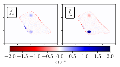
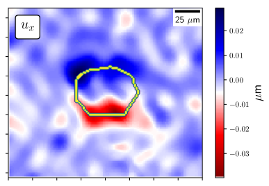
To apply our method on high-resolution experimental data, we consider the displacements resulting from stress generated by a single isolated mesenchymal stem cell. The surface displacements were measured using Hilbert space dynamometry which uses phase information of the periodic signal arising from a chemically patterned grid on the substrate [14]. In the preliminary dataset shown in Fig. 8, only $x$-displacements at a resolution of the patterned grid spacing were measured. As we have done for the simulation data in Fig. 3, the $\lambda-$optimal results for the reconstructed stress field $\hat{{\bf f}}$ using the experimental data and the full set of constraints are shown in Fig. 9.

Figure 8: Mesenchymal stem cell displacement field. Measured along $\hat{x}$ (the horizontal axis). Boundary of the cell (yellow) was hand-drawn based on bright-field image of the cell. Courtesy of G. Popescu (UIUC).

Figure 9: Reconstruction of experimental surface stress field. Reconstruction of ${\bf f}$ from the measured displacements shown in Fig. 8 using the norms defined in the manuscript. In each case, $\lambda$ was chosen using the L-curve method as described in Appendix D of the Supplementary Material.

Figure 10: False footprint constraint. Comparing the surface force reconstruction using the estimated cell footprint (from the bright field image) with the reconstruction derived from a false cell footprint. Since the forces are concentrated near the cell border, the reconstruction is sensitive to the location of the border (recall that only one direction of the displacement field was available).

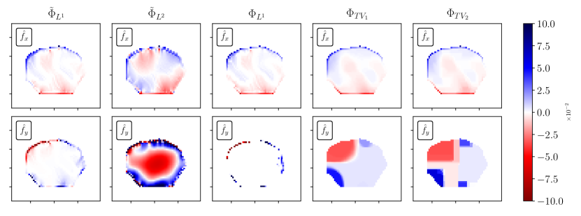
In contrast with our simulated example, these results are highly dependent on the choice of regularization. They also illustrate the importance of using isotropic regularization, particularly in reconstruction problems using these type of data where only unidirectional displacements are available. In the reconstructions using anisotropic penalties, the forces are qualitatively distinct along the two directions. This behavior is undesirable as it appears that the choice of observation axis heavily influences the outcome of the reconstruction procedure. The isotropic $L^{1}$ norm, by contrast, is robust.

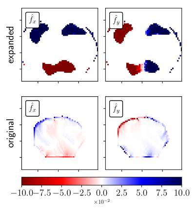
As evident from the reconstructions, the surface forces are concentrated near the border of the cell footprint. For such boundary-dominated stress fields, the footprint constraint is expected to be important in the recovery of ${\bf f}$. Fig. 10 compares the reconstruction with that computed with an artificially expanded footprint. Using an incorrect footprint results in a force distribution $\hat{{\bf f}}$ that differs from the “true” distribution, especially near the borders. Particularly, the qualitative properties of the reconstruction are markedly different when not imposing the true footprint.

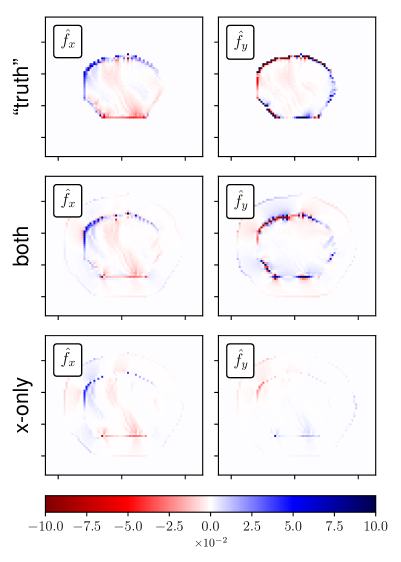
To further probe the influence of footprint specification on the reconstruction of traction forces, we assumed that our isotropic-L¹-reconstructed ($\tilde{\Phi}_{L^{1}}$) stress field is the “true” stress field, used it to generate displacements, and attempted to replicate it using the expanded (and “false”) cell boundary of Fig. 10. In this exercise, we added noise of magnitude $10^{-5}\mu$m, to approximate the noise in the real data.

The reconstruction results are shown in Fig. 11. In these reconstructions we assumed that we had available either both components of the displacement, or only a single component ($x$-only). In the case where both displacements are available (middle row), the reconstruction looks similar to that of the assumed true stress field, with the stress highly concentrated on the actual cell boundary, without explicit specification of this boundary. However, there is some leakage of forces outside of the actual boundary as well, with some forces concentrated out on the rim of the expanded false boundary.

When only a single component of the displacements is used, the reconstructed stress distribution does not gather near the actual cell boundary (Fig. 11, bottom row). The forces outside of the actual cell boundary are of similar magnitude to the forces within the cell in these reconstructions, particularly in the reconstruction of the forces in the $\hat{y}$ component. In that component, very little of the actual cell boundary is reconstructed.

Figure 11: Influence of boundary specification on force reconstruction. In the top row, we take the original reconstruction (the first columns in Figs. 9 and 10) as the new ground “truth.” Using this “true” stress field to generate displacements, we try to recover this “true” stress field, using a false footprint boundary. If both components of the displacement field are used, reasonable reconstruction is achieved (middle row). However, if only the $x$-component of the displacements are used, the reconstruction with the false expanded boundary constraint fails to detect the stress localized to the “true” boundary.

V Discussion

We presented a systematic real-space approach to solving the inverse problem associated with the reconstruction–from displacements of the underlying substrate–of surface stresses imparted by isolated cells. Our approach combines sparsity-favoring regularization, all appropriate physical constraints, and an accurate piecewise affine approximation of the exact solution to the forward problem as a system of linear equations. This approximation to the forward problem is used in a data mismatch term $\Phi_{\rm data}$ (Eq. 4). In the numerical implementation of the optimization problem, we also motivated the use of a cut-off in the solution of the forward problem that greatly reduces the rank of the inverse problem thereby decreasing both the computational complexity of the problem and the memory requirements. This cut-off approach is appropriate only in scenarios in which the stress-generating cell is localized and far from the system boundaries. Assays in which cells or layers that extend to the boundary of the sample, or in which the substrate is of finite depth will require the careful implementation of boundary conditions defined by the sample size.

Upon further consideration of physical and geometric aspects of the problem, we motivated additional important terms the objective function. The fundamental optimization problem involves minimizing an objective function containing $L^{1}$ regularization terms that are invariant to coordinate rotation. The anisotropy of $\hat{{\bf f}}$ derives solely from the anisotropy in the data. Although $L^{1}$ regularization has been used in traction force microscopy [17], in this work we also imposed a number of important physical and geometric constraints including vanishing net force/net torque and zero stress outside the cell footprint. Through exploration of the mathematical features of the stress inference problem, we find that properly identifying and implementing physical constraints (such as no-force and no-torque) are crucial to accurate stress recovery.

We also showed the footprint boundary constraint can critically impact the reconstruction, especially when adhesion sites are distributed near the cell boundary. Such boundary-localized focal adhesion configurations are commonly observed in cells grown on 2D substrates. In general, cell boundaries that artificially extend beyond the true footprint worsens the inversion, allowing for “leakage” of stress beyond its actual support. These effects are especially pronounced in reconstructions using only single-component displacement data.

For surface stress distributions that are sparse and that arise from localized focal adhesions, it is also important to use a footprint that circumscribes all sources of stress. This is especially important for cells that emanate long thin protrusions or filopodia that may be difficult to image. Indeed, the full problem may be extended to include the footprint as a variable in the objective function to be minimized. In this way, the bright field image can also be used as data automatically infer the segmentation of the footprint. A similar extension extension can be implemented to reconstruct the elastic parameters if they are not known with high certainty, resulting in a fully automated inverse problem that utilizes both imaging and substrate displacements.

Acknowledgments: This work was supported in part by the Intramural Research Program of the NIH Clinical Center and by grants from the NSF (DMS-1516675) and the Army Research Office (W911NF-14-1-0472). We are especially grateful to G. Popescu for sharing their preliminary data on cell-induced substrate deformation measured using Hilbert phase dynamometry.

VI References

Supplementary Material: Mathematical Appendices

Appendix A: Elastic Green’s function

For completeness, we explicitly list the components of the Green’s tensor for a linear elastic substrate [24]

$$G_{ss}(x,y,z)=\frac{1+\nu}{2\pi E}\left[\frac{2(1-\nu)R_{\perp}-z}{R_{\perp}(R_{\perp}-z)}+\frac{[2R_{\perp}(\nu R_{\perp}-z)+z^{2}]s^{2}}{R_{\perp}^{3}(R_{\perp}-z)^{2}}\right],$$ (A1)

$$G_{zz}(x,y,z)=\frac{1+\nu}{2\pi E}\left(\frac{2(1-\nu)}{R_{\perp}}+\frac{z^{2}}{R_{\perp}^{3}}\right),$$ (A2)

$$G_{xy}(x,y,z)=G_{yx}=\frac{1+\nu}{2\pi E}\frac{[2R_{\perp}(\nu R_{\perp}-z)+z^{2}]xy}{R_{\perp}^{3}(R_{\perp}-z)^{2}},$$ (A3)

$$G_{sz,zs}(x,y,z)=\frac{1+\nu}{2\pi E}\left(\frac{sz}{R_{\perp}^{3}}\pm\frac{(1-2\nu)s}{R_{\perp}(R_{\perp}-z)}\right).$$ (A4)

where $s\equiv x,y$. The last equation with $\pm$ corresponds to $G_{sz}$ and $G_{zs}$, respectively, and $R_{\perp}\equiv\sqrt{x^{2}+y^{2}}$. The Young’s modulus and Poisson ratio of the elastic substrate are denoted by $E$ and $\nu$, respectively.

Appendix B: Displacements and stresses at discrete positions

Here, we show the explicit expressions relating displacements ${\bf u}(x_{n},y_{m})=\boldsymbol{\Gamma}{\bf f}$ at grid points $(x_{n},y_{m})$ in terms of stress fields at the same locations. Using the interpolation of ${\bf f}(x,y)$ defined by Eq. 5 in Eq. 3, we find

$$u_{x}(x_{n},y_{m})=$$

$$\quad\sum_{(x_{j},y_{k})\in\Omega}\Bigg{\{}\Bigg{[}f_{x}(x_{j},y_{k})-x_{j}\left(\frac{f_{x}(x_{j+1},y_{k})-f_{x}(x_{j-1},y_{k})}{2\delta x}\right)-y_{k}\left(\frac{f_{x}(x_{j},y_{k+1})-f_{x}(x_{j},y_{k-1})}{2\delta y}\right)\Bigg{]}{\langle G_{xx}\rangle}^{nmjk}$$

$$\qquad\qquad+\left[\frac{f_{x}(x_{j+1},y_{k})-f_{x}(x_{j-1},y_{k})}{2\delta x}\right]\langle xG_{xx}\rangle^{nmjk}+\left[\frac{f_{x}(x_{j},y_{k+1})-f_{x}(x_{j},y_{k-1})}{2\delta y}\right]\langle yG_{xx}\rangle^{nmjk}$$

$$\qquad\qquad+\Bigg{[}f_{y}(x_{j},y_{k})-x_{j}\left(\frac{f_{y}(x_{j+1},y_{k})-f_{y}(x_{j-1},y_{k})}{2\delta x}\right)-y_{k}\left(\frac{f_{y}(x_{j},y_{k+1})-f_{y}(x_{j},y_{k-1})}{2\delta y}\right)\Bigg{]}\langle G_{xy}\rangle^{nmjk}$$

$$\qquad\qquad+\left[\frac{f_{y}(x_{j+1},y_{k})-f_{y}(x_{j-1},y_{k})}{2\delta x}\right]\langle xG_{xy}\rangle^{nmjk}+\left[\frac{f_{y}(x_{j},y_{k+1})-f_{y}(x_{j},y_{k-1})}{2\delta y}\right]\langle yG_{xy}\rangle^{nmjk}\Bigg{\}},$$ (B1)

where

$$\langle g(x,y)G_{uv}\rangle^{nmjk}=\int_{y_{k}-\delta y/2}^{y_{k}+\delta y/2}\int_{x_{j}-\delta x/2}^{x_{j}+\delta x/2}g(x^{\prime},y^{\prime})G_{uv}(x_{n}-x^{\prime},y_{m}-y^{\prime})\mbox{d}x^{\prime}\mbox{d}y^{\prime},$$ (B2)

except that at the edges where we use one-sided differences so that we are only differentiating within $\Omega$. A similar expression can be found for solving for $u_{y}$ (not shown). Collecting terms, we write $u_{x,y}(x_{n},y_{m})$ in terms of ${\bf f}(x_{j},y_{k})$ in Eq. 6, where

$$\Gamma_{xx}^{nmjk} =\langle G_{xx}\rangle^{nmjk}-\langle G_{xx}\rangle^{n,m,j-1,k}\frac{x_{j-1}}{2\delta x}+\langle G_{xx}\rangle^{n,m,j+1,k}\frac{x_{j+1}}{2\delta x}-\langle G_{xx}\rangle^{n,m,j,k-1}\frac{y_{k-1}}{2\delta y}$$

$$\quad+\langle G_{xx}\rangle^{n,m,j,k+1}\frac{y_{k+1}}{2\delta y}-\frac{\langle xG_{xx}\rangle^{n,m,j-1,k}}{2\delta x}+\frac{\langle xG_{xx}\rangle^{n,m,j+1,k}}{2\delta x}-\frac{\langle yG_{xx}\rangle^{n,m,j,k-1}}{2\delta y}+\frac{\langle yG_{xx}\rangle^{n,m,j,k+1}}{2\delta y},$$ (B3)

$$\Gamma_{xy}^{nmjk} =\langle G_{xy}\rangle^{nmjk}-\langle G_{xy}\rangle^{n,m,j-1,k}\frac{x_{j-1}}{2\delta x}+\langle G_{xy}\rangle^{n,m,j+1,k}\frac{x_{j+1}}{2\delta x}-\langle G_{xy}\rangle^{n,m,j,k-1}\frac{y_{k-1}}{2\delta y}$$

$$\quad+\langle G_{xy}\rangle^{n,m,j,k+1}\frac{y_{k+1}}{2\delta y}-\frac{\langle xG_{xy}\rangle^{n,m,j-1,k}}{2\delta x}+\frac{\langle xG_{xy}\rangle^{n,m,j+1,k}}{2\delta x}-\frac{\langle yG_{xy}\rangle^{n,m,j,k-1}}{2\delta y}+\frac{\langle yG_{xy}\rangle^{n,m,j,k+1}}{2\delta y}.$$ (B4)

Explicit closed-form expressions for the integrals in Eq. B2 are given below. By defining $\Delta x_{nj}^{+}=x_{n}-(x_{j}+\delta x/2),$ $\Delta x_{nj}^{-}=x_{n}-(x_{j}-\delta x/2)$, $\Delta y_{mk}^{+}=y_{m}-(y_{k}+\delta y/2)$, and $\Delta y_{mk}^{+}=y_{m}-(y_{k}-\delta y/2)$, we find

$$\langle G_{uv}\rangle^{nmjk} =g_{uv}(\Delta x_{nj}^{+},\Delta y_{mk}^{+})-g_{uv}(\Delta x_{nj}^{+},\Delta y_{mk}^{-})-g_{uv}(\Delta x_{nj}^{-},\Delta y_{mk}^{+})+g_{uv}(\Delta x_{nj}^{-},\Delta y_{mk}^{-})$$ (B5)

where

$$g_{xx}(x,y) =\frac{\nu+1}{\pi E}\Bigg{[}x(1-\nu)\log\left(\sqrt{x^{2}+y^{2}}+y\right)+y\log\left(\sqrt{x^{2}+y^{2}}+x\right)-y\Bigg{]}$$ (B6)

$$g_{yy}(x,y) =\frac{\nu+1}{\pi E}\Bigg{[}y(1-\nu)\log\left(\sqrt{x^{2}+y^{2}}+x\right)+x\log\left(\sqrt{x^{2}+y^{2}}+y\right)-x\Bigg{]}$$ (B7)

$$g_{xy}(x,y) =-\frac{\nu(\nu+1)}{\pi E}\sqrt{x^{2}+y^{2}}.$$ (B8)

The first moments are

$$\langle xG_{xx}(x,y)\rangle^{nmjk} =\Big{[}g_{xx}(\Delta x_{nj}^{+},\Delta y_{mk}^{+})-g_{xx}(\Delta x_{nj}^{+},\Delta y_{mk}^{-})-g_{xx}(\Delta x_{nj}^{-},\Delta y_{mk}^{+})+g_{xx}(\Delta x_{nj}^{-},\Delta y_{mk}^{-})\Big{]}x_{n}$$

$$\qquad-\Big{[}g^{x}_{xx}(\Delta x_{nj}^{+},\Delta y_{mk}^{+})-g^{x}_{xx}(\Delta x_{nj}^{+},\Delta y_{mk}^{-})-g^{x}_{xx}(\Delta x_{nj}^{-},\Delta y_{mk}^{+})+g^{x}_{xx}(\Delta x_{nj}^{-},\Delta y_{mk}^{-})\Big{]},$$ (B9)

where

$$g^{x}_{xx}(x,y) =\frac{\nu+1}{2\pi E}\Big{[}(\nu+1)y\sqrt{x^{2}+y^{2}}-(\nu-1)x^{2}\log\left(\sqrt{x^{2}+y^{2}}+y\right)\Big{]},$$ (B10)

$$\langle yG_{xx}(x,y)\rangle^{nmjk} =\Big{[}g_{xx}(\Delta x_{nj}^{+},\Delta y_{mk}^{+})-g_{xx}(\Delta x_{nj}^{+},\Delta y_{mk}^{-})-g_{xx}(\Delta x_{nj}^{-},\Delta y_{mk}^{+})+g_{xx}(\Delta x_{nj}^{-},\Delta y_{mk}^{-})\Big{]}y_{m}$$

$$\qquad-\Big{[}g^{y}_{xx}(\Delta x_{nj}^{+},\Delta y_{mk}^{+})-g^{y}_{xx}(\Delta x_{nj}^{+},\Delta y_{mk}^{-})-g^{y}_{xx}(\Delta x_{nj}^{-},\Delta y_{mk}^{+})+g^{y}_{xx}(\Delta x_{nj}^{-},\Delta y_{mk}^{-})\Big{]},$$ (B11)

where

$$g^{y}_{xx}(x,y) =\frac{\nu+1}{2\pi E}\Bigg{[}y^{2}\log\left(\sqrt{x^{2}+y^{2}}+x\right)-\sqrt{x^{2}+y^{2}}\left((2\nu-1)x+\frac{1}{2}\sqrt{x^{2}+y^{2}}\right)\Bigg{]},$$ (B12)

and

$$\langle xG_{xy}(x,y)\rangle^{nmjk} =\Big{[}g_{xy}(\Delta x_{nj}^{-},\Delta y_{mk}^{+})-g_{xy}(\Delta x_{nj}^{-},\Delta y_{mk}^{-})-g_{xy}(\Delta x_{nj}^{+},\Delta y_{mk}^{+})+g_{xy}(\Delta x_{nj}^{+},\Delta y_{mk}^{-})\Big{]}x_{n}$$

$$\qquad-\Big{[}g_{xy}^{x}(\Delta x_{nj}^{+},\Delta y_{mk}^{+})-g_{xy}^{x}(\Delta x_{nj}^{+},\Delta y_{mk}^{-})-g_{xy}^{x}(\Delta x_{nj}^{-},\Delta y_{mk}^{+})+g_{xy}^{x}(\Delta x_{nj}^{-},\Delta y_{mk}^{-})\Big{]}$$ (B13)

where

$$g_{xy}^{x}(x,y) =\frac{\nu(\nu+1)}{\pi E}\Big{[}\frac{y^{2}}{2}\log\left(\sqrt{x^{2}+y^{2}}+x\right)-\frac{1}{4}\sqrt{x^{2}+y^{2}}\left(\sqrt{x^{2}+y^{2}}+2x\right)\Big{]}.$$ (B14)

Analogous expressions are straightforwardly derived for $\Gamma_{yx}^{nmjk}$ and $\Gamma_{yy}^{nmjk}$.

All of the above expressions may be found through direct iterated evaluation of the integrals, as long as $n\neq m$ or $j\neq k$ the integrand (effectively the Green’s function) is bounded, hence making Fubini’s theorem applicable given the compactly supported domains of integration.

In the special case where $n=m$ and $j=k$, these formulae also hold. This fact is found by decomposing the integration domain to exclude the origin, for instance in the manner

$$\int_{-\Delta y/2}^{\Delta y/2}\int_{-\Delta x/2}^{\Delta x/2}{\bf d}{\bf r}=\lim_{\varepsilon\to 0}\left(\int_{\varepsilon}^{\Delta y/2}+\int_{-\Delta y/2}^{\varepsilon}\right)\int_{\Delta x/2}^{\Delta x/2}{\bf d}{\bf r}.~{}$$ (B15)

Since the antiderivatives of Eqs. B6, B7, B8, B10, B12, and B14 all have well-defined limits with only removable discontinuities at the origin, integrals of the Green’s functions defined through Eq. B15 all converge about the origin and the equations above also hold in the case where $n=m$ and $j=k$. These explicit expressions allow us to accurately evaluate ${\bf u}({\bf r}_{i})$ in $\Phi_{\rm data}[{\bf f}]$.

Appendix C: Decay of displacement fields

Note that $u_{x}$ and $u_{y}$ are symmetric in form. Hence, it will suffice to prove just one of these assertions. Eq. 3 can be written as

$$u_{x}({\bf r}) =\frac{1+\nu}{\pi E}\int\frac{\mbox{d}{\bf r}}{|{\bf r}-{\bf r}^{\prime}|}\Bigg{\{}\left[\frac{\nu(x-x^{\prime})^{2}}{|{\bf r}-{\bf r}^{\prime}|^{2}}+1-\nu\right]f_{x}({\bf r}^{\prime})+\nu\frac{(x-x^{\prime})(y-y^{\prime})}{|{\bf r}-{\bf r}^{\prime}|^{2}}f_{y}({\bf r}^{\prime})\Bigg{\}}$$

$$\equiv\frac{1+\nu}{\pi E}\int\frac{\rho_{x}({\bf r},{\bf r}^{\prime})}{|{\bf r}-{\bf r}^{\prime}|}\mbox{d}{\bf r}^{\prime}$$ (C1)

where $\rho_{x}({\bf r},{\bf r}^{\prime})$ is $\mathcal{O}(1)$ as $|{\bf r}|\to\infty$. Without loss of generality, we assume that the coordinate system is centered at some point $\mathbf{0}\in\Omega$. The Euclidean distances can then be represented through the binomial expansion,

$$\frac{1}{|{\bf r}-{\bf r}^{\prime}|^{p}} =\frac{1}{|{\bf r}|^{p}}\frac{1}{\left(1-\frac{2{\bf r}\cdot{\bf r}^{\prime}}{|{\bf r}|^{2}}+\frac{|{\bf r}^{\prime}|^{2}}{|{\bf r}|^{2}}\right)^{p/2}}=\frac{1}{|{\bf r}|^{p}}\sum_{k=0}^{\infty}{{{p\over 2}+k-1}\choose{k}}{\left(\underbrace{\frac{2{\bf r}\cdot{\bf r}^{\prime}-|{\bf r}^{\prime}|^{2}}{|{\bf r}|^{2}}}_{\mathcal{O}(|{\bf r}|^{-1})}\right)}^{k}.$$ (C2)

Since ${\bf r}\not\in\Omega$ and ${\bf r}^{\prime}\in\Omega$, the series converges in the $|{\bf r}|\to\infty$ limit. Plugging this series into the last line of Eq. C1, where $p=1$, one sees that it in order to show that the magnitude of $u_{x}({\bf r})$ is $\mathcal{O}(|{\bf r}|^{-q})$, it suffices to show that $\int\rho({\bf r},{\bf r}^{\prime})\mbox{d}{\bf r}^{\prime}\leq{\cal O}(|{\bf r}|^{-q+1})$.

Using the fact that $\int{\bf f}({\bf r}){\bf d}{\bf r}=\mathbf{0}$, one finds that

$$\int\rho_{x}({\bf r},{\bf r}^{\prime}){\bf d}{\bf r}^{\prime} =\int(1-\nu)f_{x}({\bf r}^{\prime}){\bf d}{\bf r}^{\prime}+\nu\int\left[\frac{(x-x^{\prime})^{2}}{|{\bf r}-{\bf r}^{\prime}|^{2}}f_{x}({\bf r}^{\prime})+\frac{(x-x^{\prime})(y-y^{\prime})}{|{\bf r}-{\bf r}^{\prime}|^{2}}f_{y}({\bf r}^{\prime})\right]{\bf d}{\bf r}^{\prime}$$

$$=\frac{\nu}{|{\bf r}|^{2}}\int\Bigg{[}(x-x^{\prime})^{2}f_{x}({\bf r}^{\prime})+(x-x^{\prime})(y-y^{\prime})f_{y}({\bf r}^{\prime})\Bigg{]}\sum_{k=0}^{\infty}\left[\frac{2{\bf r}\cdot{\bf r}^{\prime}-|{\bf r}^{\prime}|^{2}}{|{\bf r}|^{2}}\right]^{k}{\bf d}{\bf r}^{\prime}.$$ (C3)

Expanding the leading order term of this expression, we see that

$$\int\rho_{x}({\bf r},{\bf r}^{\prime}){\bf d}{\bf r} =\frac{\nu}{|{\bf r}|^{2}}\int\Bigg{[}(x-x^{\prime})^{2}f_{x}({\bf r}^{\prime})+(x-x^{\prime})(y-y^{\prime})f_{y}({\bf r}^{\prime})\Bigg{]}{\bf d}{\bf r}^{\prime}$$

$$=\frac{\nu}{|{\bf r}|^{2}}\Bigg{[}-2x\int x^{\prime}f_{x}({\bf r}^{\prime}){\bf d}{\bf r}^{\prime}+\int x^{\prime 2}f_{x}({\bf r}^{\prime}){\bf d}{\bf r}^{\prime}-x\int y^{\prime}f_{y}({\bf r}^{\prime}){\bf d}{\bf r}^{\prime}-y\int x^{\prime}f_{y}({\bf r}^{\prime}){\bf d}{\bf r}^{\prime}+\int x^{\prime}y^{\prime}f_{y}({\bf r}^{\prime}){\bf d}{\bf r}^{\prime}\Bigg{]}$$

$$=\mathcal{O}(|{\bf r}|^{-1}).$$ (C4)

Hence, it is evident that this integral is of $\mathcal{O}(|{\bf r}|^{-2})$, where to the leading order we have

$$u_{x}({\bf r})=\frac{1+\nu}{\pi E|{\bf r}|^{2}}\Bigg{[}-2\nu\frac{x}{|{\bf r}|}\int x^{\prime}f_{x}({\bf r}^{\prime}){\bf d}{\bf r}^{\prime}-\frac{x\nu}{|{\bf r}|}\int y^{\prime}f_{y}({\bf r}^{\prime}){\bf d}{\bf r}^{\prime}$$

$$\qquad-\frac{y\nu}{|{\bf r}|}\int x^{\prime}f_{y}({\bf r}^{\prime}){\bf d}{\bf r}^{\prime}+(1-\nu)\frac{{\bf r}}{|{\bf r}|}\cdot\int{\bf r}^{\prime}f_{x}({\bf r}^{\prime}){\bf d}{\bf r}^{\prime}\Bigg{]}+\mathcal{O}(|{\bf r}|^{-3}).$$ (C5)

Appendix D: Choice of regularization penalty parameter $\lambda$

The “L-curve” below illustrates the optimal choice of $\lambda$ for each reconstruction used in this paper.

List of suppfigures 1 Choice of $\lambda$ by plotting the tradeoff between regularity and data mismatch for different values of $\lambda$. The “optimal” value (red circle) is chosen by to be the point farthest away from the line segment joining the two ends of the plot (green and black circles). Reconstructions under the different values of $\lambda$ given by these circles are shown. The green circle corresponds to solution with low regularity and is hence “under-regularized.” The black circle coincides with a solution of high regularity and is hence “over-regularized.”

List of suppfigures 2 Choice of $\lambda$ for mesenchymal cell data (where displacements are known only in one direction). The optimal reconstruction corresponds to the elbow of the tradeoff curve. Color contrast enhanced relative to scale used in the manuscript body.

References

- [1] Masha Prager-Khoutorsky, Alexandra Lichtenstein, Ramaswamy Krishnan, Kavitha Rajendran, Avi Mayo, Zvi Kam, Benjamin Geiger, and Alexander D. Bershadsky. Fibroblast polarization is a matrix-rigidity-dependent process controlled by focal adhesion mechanosensing. Nature Cell Biology, 13:1457–1465, 2011.
- [2] Tim Pieters and Frans van Roy. Role of cell–cell adhesion complexes in embryonic stem cell biology. Journal of Cell Science, 127:2603–2613, 2014.
- [3] Andy Aman and Tatjana Piotrowski. Cell migration during morphogenesis. Developmental Biology, 341:20–33, 2010.
- [4] L. Schneider, M. Cammer, J. Lehman, S. K. Nielsen, C. F. Guerra, I. R. Veland, C. Stock, E. K. Hoffmann, B. K. Yoder, A. Schwab, P. Satir, and S. T. Christensen. Directional Cell Migration and Chemotaxis in Wound Healing Response to PDGF-AA are Coordinated by the Primary Cilium in Fibroblasts. Cell Physiology and Biochemistry, 25:279–292, 2010.
- [5] Li Li, Yong He, Min Zhao, and Jianxin Jiang. Collective cell migration: Implications for wound healing and cancer invasion. Burns and Trauma, 1:21–26, 2013.
- [6] Mariaceleste Aragona, Sophie Dekoninck, Steffen Rulands, Sandrine Lenglez, Guilhem Mascré, Benjamin D. Simons, and Cédric Blanpain. Defining stem cell dynamics and migration during wound healing in mouse skin epidermis. Nature Communications, 8:14684, 2017.
- [7] Andrew G. Clark and Danijela Matic Vignjevic. Modes of cancer cell invasion and the role of the microenvironment. Current Opinion in Cell Biology, 36:13–22, 2015.
- [8] James Watson, Bruce Alberts, Dennis Bray, Martin Raff, and Julian Lewis. Molecular Biology of the Cell, 6th Edition. Garland Science, 2014.
- [9] John L. Tan, Joe Tien, Dana M. Pirone, Darren S. Gray, Kiran Bhadriraju, and Christopher S. Chen. Cells lying on a bed of microneedles: An approach to isolate mechanical force. Proceedings of The National Academy of Sciences USA, 100:1484–1489, 2003.
- [10] Nathalie Q. Balaban, Ulrich S. Schwarz, Daniel Riveline, Polina Goichberg, Gila Tzur, Ilana Sabanay, Diana Mahalu, Sam Safran, Alexander Bershadsky, Lia Addadi, and Benjamin Geiger. Force and focal adhesion assembly: a close relationship studied using elastic micropatterned substrates. Nature Cell Biology, 3:466–472, 2001.
- [11] James H.-C. Wang and Jeen-Shang Lin. Cell traction force and measurement methods. Biomechanics and Modeling in Mechanobiology, 6:361–371, 2007.
- [12] B. Sabass, M. L. Gardel, C. M. Waterman, and U. S. Schwarz. High resolution traction force microscopy based on experimental and computational advances. Biophysical Journal, 94:207–220, 2008.
- [13] Huw Colin-York, Christian Eggeling, and Marco Fritzsche. Dissection of mechanical force in living cells by super-resolved traction force microscopy. Nature Protocols, 12:783–796, 2017.
- [14] Shamira Sridharana, Yanfen Li, Louis Foucarde, Hassaan Majeed, Basanta Bhaduria, Alex J. Levine, Kristopher Kilian, and Gabriel Popescu. Hilbert phase dynamometry for real-time cell traction imaging. Submitted: Nature Methods, 2017.
- [15] Tom Goldstein and Stanley Osher. The Split Bregman Method for L1-Regularized Problems. SIAM J. Imaging Sciences, 2:323–343, 2009.
- [16] Tony F. Chan and S. Esedoglu. Aspects of total variation regularized function approximation. SIAM J. Appl. Math., 65:1817–1837, 2004.
- [17] Sangyoon J Han, Youbean Oak, Alex Groisman, and Gaudenz Danuser. Traction microscopy to identify force modulation in subresolution adhesions. Nature Methods, 12:953–656, 2015.
- [18] Shauheen S. Soofia, Julie A. Lasta, Sara J. Liliensieka, Paul F. Nealey, and Christopher J. Murphy. The elastic modulus of Matrigel as determined by atomic force microscopy. Journal of Structural Biology, 167:216–219, 2009.
- [19] J. C. Chang, V. M. Savage, and T. Chou. A path-integral approach to Bayesian inference for inverse problems using the semiclassical approximation. Journal of Statistical Physics, 157(3):582–602, 2014.
- [20] James P. Butler, Iva Marija Tolić-Nørrelykke, Ben Fabry, and Jeffrey J. Fredberg. Traction fields, moments, and strain energy that cells exert on their surroundings. American Journal of Physiology - Cell Physiology, 282:C595–C605, 2002.
- [21] J. C. Chang, P.-W. Fok, and T. Chou. Bayesian uncertainty quantification for bond energies and mobilities using path integral analysis. Biophysical Journal, 109:966–974, 2015.
- [22] S. V. Plotnikov, B. Sabass, U. S. Schwarz, and C. M. Waterman. High-resolution traction force microscopy. Methods in Cell Biology, 123:367–394, 2014.
- [23] Steven Diamond and Stephen Boyd. CVXPY: A Python-embedded modeling language for convex optimization. Journal of Machine Learning Research, 17(83):1–5, 2016.
- [24] L. D. Landau and E. M. Lifshitz. Theory of Elasticity. Pergamon Press, Oxford, 1970.