Families of non-linear subdivision schemes for scattered data fitting and their non-tensor product extensions
Abstract
In this article, families of non-linear subdivision schemes are presented that are based on univariate polynomials up to degree three. Theses families of schemes are constructed by using dynamic iterative reweighed least squares method. These schemes are suitable for fitting scattered data with noise and outliers. Although these schemes are non-interpolatory, but have the ability to preserve the shape of the initial polygon in case of non-noisy initial data. The numerical examples illustrate that the schemes constructed by non-linear polynomials give better performance than the schemes that are constructed by linear polynomials (Computer-Aided Design, 58, 189-199). Moreover, the numerical examples show that these schemes have the ability to reproduce polynomials and do not cause over and under fitting of the data. Furthermore, families of non-linear bivariate subdivision schemes are also presented that are based on linear and non-linear bivariate polynomials.
Keywords:
Subdivision scheme; Iterative re-weighted least squares method; -regression; Noisy data; Outlier; Reproduction; Over and under fitting;
AMS Subject Classifications: 65D17; 65D10; 68U07; 93E24; 62J02; 62J05
1 Introduction
Curve fitting is the method of constructing a curve, or a mathematical function, that has the best fit to a series of data points, probably subject to constraints. In statistics and machine learning, the common task is to fit a ”model” to a set of training data, so as to be able to make consistent predictions on general untrained data. The cause of poor performance in statistics and machine learning is either overfitting or underfitting the data. In overfitting, a statistical model describes random error or noise instead of the underlying relationship. Overfitting occurs when a model is extremely complex, such as owning too many parameters relative to the number of observations. A model that has been overfit has poor predictive performance, as it overreacts to small variations in the training data. For example, the presence of outliers in the initial data points may increase the chance of overfitting in the fitted curves. Underfitting happens when a statistical model or machine learning algorithm cannot capture the underlying trend of the data. It occurs when the model or algorithm does not fit the data enough. It is often a result of an extremely simple model. For example, when fitting a linear model to non-linear data. Such a model would have poor predictive performance.
The method of least squares is one of the wonderful technique in statistics for curves fitting, whereas in the field of geometric modeling subdivision schemes are used for curves and surfaces fitting. Subdivision schemes are recursive processes used for the quick generation of curves and surfaces. Subdivision schemes are also important ingredients in many multiscale algorithms used in data compression. In some applications, the given data need not to be retained at each step of the refinement process, which requires the use of approximating subdivision schemes. Nowadays, approximating subdivision schemes are further categorized as classical schemes and least squares subdivision schemes. Many authors in the field of geometric modeling have been constructed classical subdivision schemes for different type of initial data. Some of the recently constructed classical schemes along with their properties are available in [5, 6, 8, 10, 12]. The detail information about these schemes can be found in [4]. Classical schemes are not suitable to fit scattered data and they are very sensitive to outliers. The presence of only one outlier in the initial data can badly damage the whole fitted model. This drawback of classical schemes has been inspired to construct least squares techniques based subdivision schemes.
The first attempt to construct subdivision schemes by using least squares technique is done by Dyn et al. [3]. They introduced univariate linear binary subdivision schemes for refining noisy data by fitting local least squares polynomials. They also give several numerical experiments to show the performance of their schemes on initial noisy data. Mustafa et al. [11] proposed the -regression based univariate and non-tensor product bivariate binary subdivision schemes to handle with noisy data with outliers. They also give many numerical experiments to determine the usability and practicality of their proposed schemes. Mustafa and Bari [9] proposed univariate and non-tensor product bivariate -ary () subdivision schemes to fit local least squares polynomials of degree 3. However, they have not given any numerical experiment to see the performance of their schemes on noisy data. The following motivation plays a vital role behind the construction of our families of schemes.
1.1 Motivation and contribution
Mustafa et al. [11] proposed subdivision schemes with dynamic iterative re-weighted weights by fitting 1D and 2D line functions to -observations and -observations in 2D and 3D spaces respectively. Their schemes have following merits:
-
•
The schemes remove noises and outliers without prior information about the input data.
-
•
Overfitting of the data does not occur by using their schemes.
But the following de-merits have been noted in the schemes based on fitting 1D and 2D line functions:
- •
- •
The above issues motivate us to present the schemes based on fitting non-linear polynomial functions. We observe the following characteristics in the schemes that are based on fitting non-linear polynomial functions:
- •
- •
- •
- •
-
•
In surface case, our schemes produce smooth models comparative to the schemes of [11].
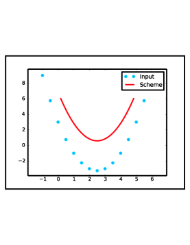 |
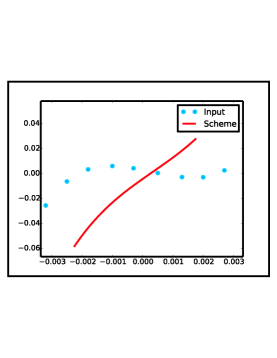 |
|
| (a) | (b) | |
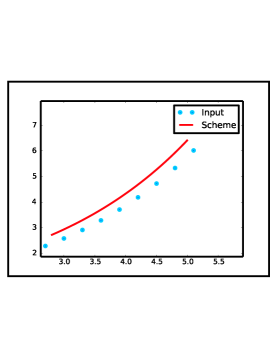 |
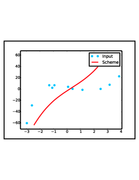 |
|
| (c) | (d) |
For better understanding of this article, we have organized the material in the following fashion. In Section 2, we give the algorithms for the construction of families of binary univariate subdivision schemes. We also construct families of univariate schemes based on -regression by using degree three, two and one polynomials respectively in this section. In Section 3, the numerical examples of the proposed families of schemes are presented. In Section 4, we construct families of bivariate subdivision schemes that are based on bivariate polynomials up to degree two. We give the conclusion of our work in Section 5.
2 Framework for the construction of univariate schemes
In this section, we present a framework for the construction of families of univariate approximating schemes. The framework has two steps. In first step, we fit the univariate -degree polynomial to the -observations/data by using the IRLS. In second step, we derive the families of -point approximating subdivision schemes also called -schemes.
2.1 Step 1
Consider the univariate polynomial function of degree
| (2.1) |
where , , are the monomial functions.
Now express the polynomial function (2.1) with respect to the observations for () as
| (2.2) |
Let , then use fitting function of [13] for estimating . The -norm operator is defined as
The optimum of is expressed as
| (2.3) | |||||
Use the IRLS method [2] which is based on the thought that, in a first step, the norm , being a convex functional, can be approximated by a family of smooth convex functionals , . That is
| (2.4) |
The regularization of the non-smooth functional (2.3) by (2.4) has been done by [14]. So by ([2], Theorem 1), we get
This means that is the approximation of .
Thus, in order to compute , use the iterative formula given below
| (2.5) |
where
| (2.6) |
Here is called the dynamic iterative weights. When , , then the -regression problem converts into the -regression problem.
The ordinary least squares method can be used to find out the starting values , i.e. determine the values of unknown parameters in (2.2) to make the sum of the squares of residuals minimum. The sum of the squares of residuals is defined as
| (2.7) |
Now differentiating (2.5) and (2.7) with respect to , then setting each system of the -equations equal to zero and then by solving these systems for unknowns values, we get the values of and respectively.
2.2 Step 2
In this step, first evaluate the best fitted -degree polynomial (2.8) at and . Then set the following notations for iterative point of view. That is, set
and also set the data values , involved in , where and are the control points at level and respectively. The refinement rules and make the families of -point -schemes denoted by to fit a curve to the set of data points. Step 2 is briefly described in Algorithm 2.
Remark 2.1.
The -ary subdivision scheme is a tool which maps a polygon/mesh to a refined mesh where denotes a sequence of points in and is a non negative integer. For and , the -ary scheme is univariate and bivariate respectively.
Furthermore, for , the and schemes mean the binary -variate -schemes computed from -variate -degree polynomial. These schemes take and consecutive points from initial polygon/mesh respectively to compute a new point in order to get a refined polygon/mesh. In other words, schemes mean the binary -variate schemes computed from -variate -degree polynomials where . From numerical experiments, it is to be noted that small value of is a good choice, while good choice of is 5 or 6.
Proposition 2.1.
Proposition 2.2.
| (2.14) | |||||
| (2.16) |
where
| (2.22) |
| (2.28) |
| (2.34) |
| (2.35) |
Proposition 2.3.
| (2.37) |
| (2.38) |
| (2.39) |
Remark 2.2.
Since from iterative point of view, we have set and . Furthermore, set the symbols used in Proposition 2.2 as for ; for and for .
2.3 Family of -point schemes based on polynomial of degree 3
From Propositions 2.1-2.2 and Algorithm 2 for , we get the following family of -point subdivision schemes based on fitting polynomial of degree 3
| (2.43) |
where
| (2.44) | |||||
| (2.45) | |||||
| (2.46) | |||||
| (2.47) | |||||
| (2.48) | |||||
2.4 Family of -point schemes based on polynomial of degree 3
We have introduced a family of schemes in (2.43) that is based on the fitting of a cubic univariate polynomial to -observations in two-dimensional space. We can get an alternative of the schemes by fitting polynomial function of degree 3 to -observations. This alternative can be obtained by replacing to in (2.13)-(2.35) and (2.43)-(2.50), by and by in (2.43). Ultimately, we get the following family of schemes denoted by
| (2.54) |
The starting values are defined in Proposition 2.3.
Now we introduce two more families of schemes that are based on fitting polynomial of degree 2.
2.5 Family of -point schemes based on polynomial of degree 2
From Propositions 2.1-2.2 with and Algorithm 2 with , we get the following family of -points schemes based on fitting polynomial of degree 2.
| (2.58) |
where is defined in (2.22) and
| (2.59) | |||||
2.6 Family of -point schemes based on polynomial of degree 2
Similarly, if we fit a polynomial function of degree two to -observations, we get a further alternative of the schemes , i.e. replace by in Proposition 2.2 and (2.58)-(2.59) and then use Propositions 2.2-2.3 for to get the following family of -point schemes
| (2.63) |
where and are defined in (2.22) and (2.59) respectively and
2.7 Families of schemes based on polynomial of degree 1
If we use Propositions 2.1-2.2 with , and Algorithm 2, we get the family of -point schemes proposed by Mustafa et al. [11]. The refinement rules of this family of schemes are
If we replace by in Proposition 2.2, then use Propositions 2.2-2.3 for and then apply Algorithm 2 for , we get the following family of schemes proposed by Mustafa et al. [11]. The family of schemes is
| (2.72) |
2.8 Basic limit functions
The basic limit functions of the families of schemes , , are defined as
where is the initial data such that for sufficiently large positive integer .
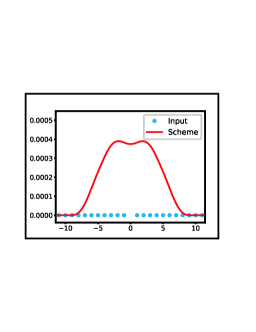
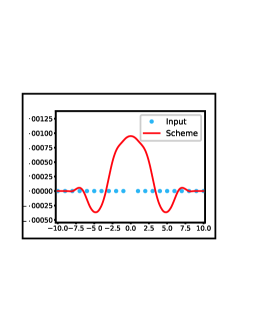
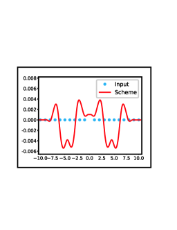
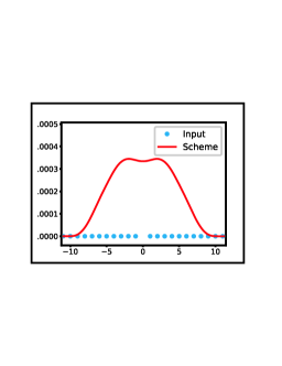
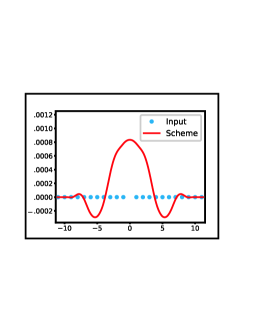
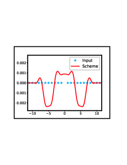
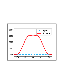
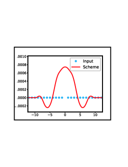
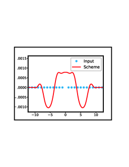
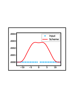
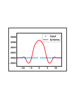
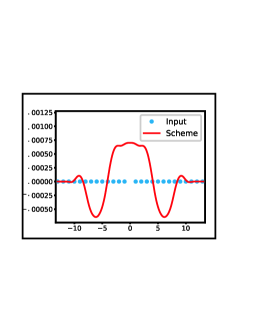
The support of the basic limit functions and the subdivision schemes is the area of the limit curve that will be affected by the displacement of a single control point from its initial place. The part which is dependent on that given control point is called the support width of that control point. By using the approach of Beccari et al. [1], it can be easily proved that the basic limit functions of families of scheme have the support width , where which implies that it vanishes out side the interval . Similarly, the basic limit functions of the families of schemes have the support width , where which implies that it vanishes out side the interval . Figure 2(a)-(l) shows the basic limit functions of the schemes , , , , , , , , , , and respectively. From this figure we see that the effects of the schemes constructed with different degree polynomials are different on initial data . The schemes and have two and one top peaks respectively , while the behavior of schemes is greatly effected with a small change in .
 |
 |
 |
|
| (a) | (b) | (c) |
 |
 |
 |
|
| (d) | (e) | (f) |
 |
 |
 |
|
| (g) | (h) | (i) |
 |
 |
 |
|
| (j) | (k) | (l) |
3 Numerical examples
In this section, we give several numerical examples to see the performance of the proposed families of schemes. Different types of initial data have been used for this purpose. We give the comparisons of the schemes based on fitting non-linear and linear polynomials.
Example 3.1.
Response to the polynomial data
According to [7], three numerical quantities indicate the behavior of a subdivision scheme when all the initial control points lie on a polynomial. The limit curves on all polynomial data up to a certain degree passes through the same polynomial, a polynomial of the same degree or passes through the original control points.
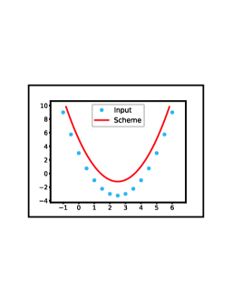
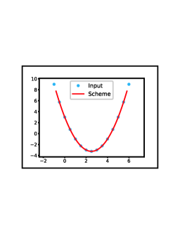
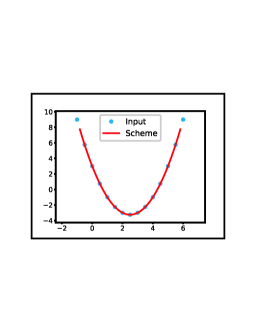
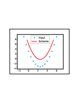
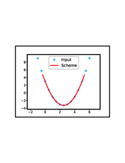
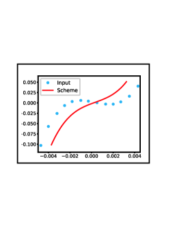
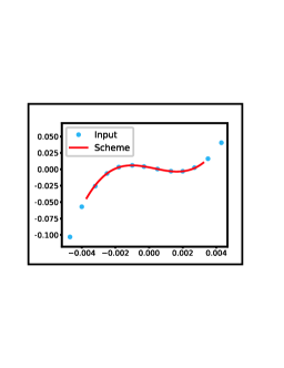
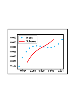
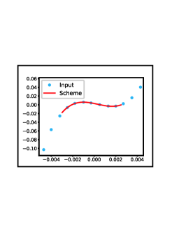
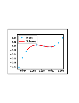
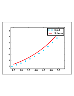
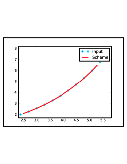
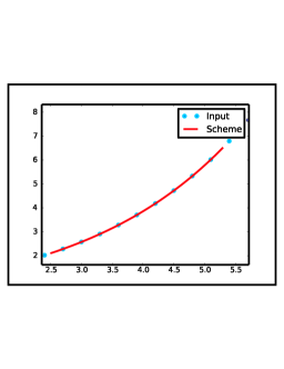
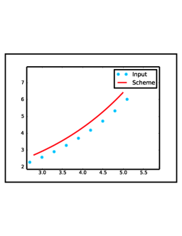
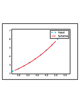
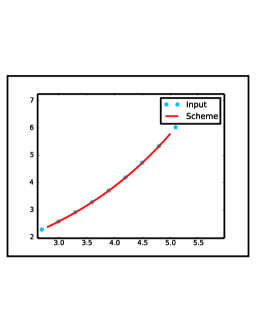
These three behaviors show three maximal degrees, that are reproduction degree, generation degree, and interpolation degree respectively. Figures 3-5 show the responses of the schemes , and , where , on the data taken from quadratic polynomial function , cubic polynomial function and exponential polynomial function respectively. We can see from these figures that fitted curves by schemes , , generate, reproduce and interpolate these polynomials while the limit curves of the schemes do not reproduce and interpolate these polynomials.
 |
 |
 |
|
| (a) | (b) | (c) |
 |
 |
 |
|
| (d) | (e) | (f) |
 |
 |
 |
|
| (a) | (b) | (c) |
 |
 |
 |
|
| (d) | (e) | (f) |
 |
 |
 |
|
| (a) | (b) | (c) |
 |
 |
 |
|
| (d) | (e) | (f) |
Example 3.2.
Response to the discontinuous data
If we generate initial data from a discontinuous function
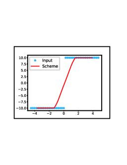
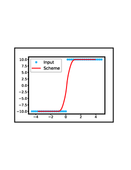
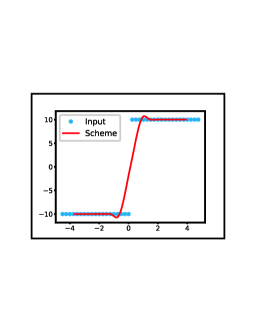
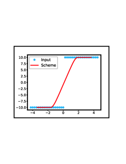
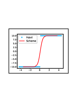
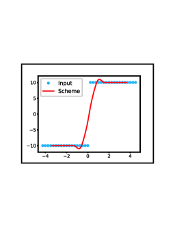
then from Figure 6 the fitted curves generated by the proposed schemes , , and do not suffer from Gibbs oscillations, whereas the curves generated by the proposed schemes and suffer from these oscillations. It means that the schemes based on higher degree polynomials are not suitable for fitting the data that comes from discontinuous functions.
 |
 |
 |
|
| (a) | (b) | (c) |
 |
 |
 |
|
| (d) | (e) | (f) |
Example 3.3.
Interpolating behavior to the non-noisy data
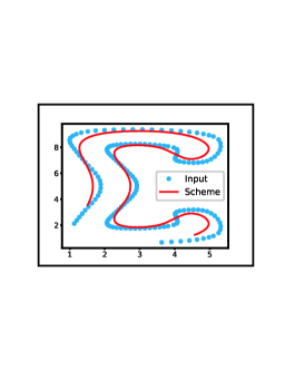
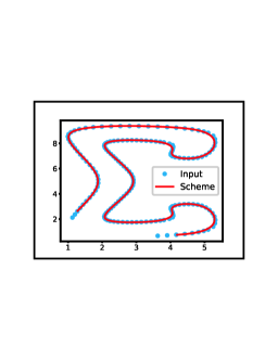
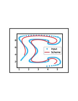
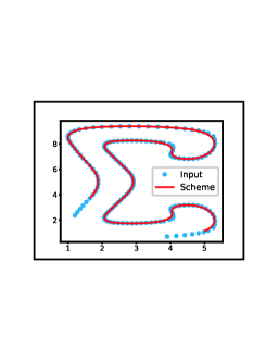
The higher complexity schemes are more suitable to handle with noisy data [11]. It is observed that the schemes generated by the higher degree polynomials, i.e , , and , show interpolatory behavior on non-noisy data points, while the schemes generated by the linear polynomial, i.e. and , show approximating behavior (see Figure 7).
 |
 |
 |
|
| (a) | (b) | (c) |
 |
 |
 |
|
| (d) | (e) | (f) |
Example 3.4.
Response to the data that contains outliers
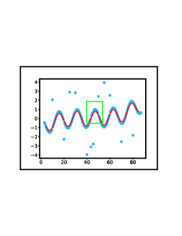
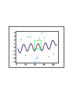
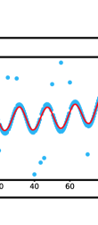
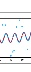
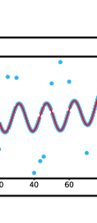
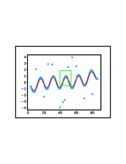
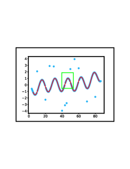
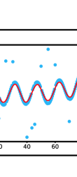
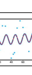
In this example, we generate data from the oscillatory function along with twelve outliers. The limit curves generated by the proposed schemes are presented in Figure 8. In this figure, blue bullets show the initial control points, while solid lines show fitted curves. This figure shows that the curves generated by the proposed schemes with and are more consistent with the graph of than the curves generated by .
 |
 |
 |
|
| (a) | (b) | (c) | |
 |
 |
 |
|
| (d) | (e) | (f) |
 |
 |
 |
|
| (g) | (h) | (i) | |
 |
 |
 |
|
| (j) | (k) | (l) |
Example 3.5.
Response to the noisy data with outliers
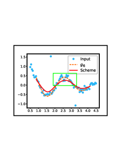
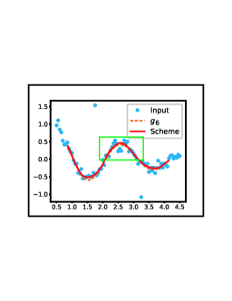
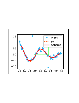
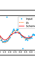
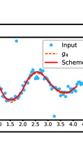
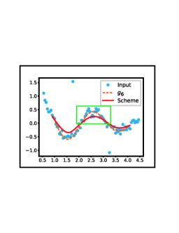
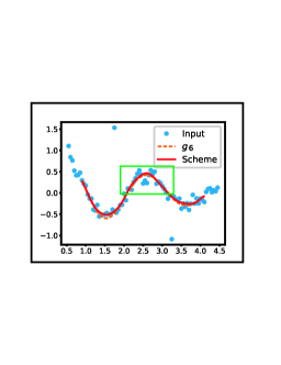
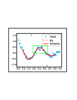
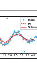
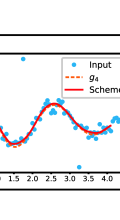
Let us take noisy data from the function with two outliers. We want to see the effects of this noisy data with outliers on the fitted curves. From Figure 9, it is to be observed that the fitted curves generated by the proposed schemes , , , , and are not effected by outliers and noise.
 |
 |
 |
|
| (a) | (b) | (c) | |
 |
 |
 |
|
| (d) | (e) | (f) |
 |
 |
 |
|
| (g) | (h) | (i) | |
 |
 |
 |
|
| (j) | (k) | (l) |
Remark 3.1.
Families of -point -ary () subdivision schemes can be obtained by substituting optimum of into degree three, two and one univariate polynomial functions and then evaluating these functions at , . Similarly, by evaluating these functions at with and with , we get families of -point even N-ary subdivision schemes and -point odd N-ary subdivision schemes respectively.
4 Framework for the construction of bivariate schemes
In this section, we generalize our representation of the 2-dimensional case to the 3-dimensional case to construct families of -point and -point non-tensor product binary schemes by using the IRLS technique as optimality criterion. Again the proposed framework contains two steps. These steps are presented in the following subsections.
4.1 Step 1
Consider the following bivariate polynomial function of degree to determine the best function to fit the data
| (4.1) |
where are the monomial functions with and , i.e. there is one one correspondence between , , , , , and ,, , , , , , , , .
The polynomial function (4.1) with respect to the observations for , where can be expressed as
| (4.2) |
The norm operator that is used for estimating is defined as
The optimum of is
| (4.3) | |||||
Use the IRLS method to approximate by () as
By regularizing (4.3) with (4.1) and using the generalized version of ([2], Theorem 1), we get
Thus, we compute which is the approximation of by using the following iterative formula
| (4.5) | |||||
where
| (4.6) |
For starting values , use the ordinary least squares method.
The sum of the squares of residuals for bivariate degree polynomial is
| (4.7) |
Differentiate (4.5) and (4.7) with respect to then solve these systems for unknowns values, we get and respectively. Iterations will continue until
Substitute in (4.2) to get the following best fitted -degree polynomial to the -observations
| (4.8) |
This step is briefly defined in Algorithm 3.
4.2 Step 2
In this step, evaluate the bivariate -degree polynomial (4.8) at , , and . Then, for the iterative point of view, set the following representations
and the 3D data values involved in are set as
where and are the control points at level and respectively. For different values of and , the four refinement rules ,, and make the -point scheme denoted by to fit a surface to the set of 3D data points.
Proposition 4.1.
| (4.10) |
| (4.11) |
| (4.12) |
| (4.13) |
| (4.14) | |||||
Proposition 4.2.
| (4.15) |
| (4.16) |
| (4.17) |
| (4.18) |
| (4.19) | |||||
| (4.20) | |||||
where
| (4.24) |
| (4.32) |
| (4.38) |
| (4.46) |
| (4.54) |
| (4.61) | |||||
| (4.62) | |||||
| (4.63) | |||||
| (4.64) | |||||
| (4.65) | |||||
| (4.66) | |||||
| (4.67) | |||||
| (4.68) | |||||
| (4.69) | |||||
| (4.70) | |||||
| (4.71) | |||||
| (4.72) | |||||
| (4.73) | |||||
| (4.74) | |||||
| (4.75) | |||||
| (4.76) | |||||
| (4.77) | |||||
| (4.78) | |||||
| (4.79) | |||||
| (4.80) | |||||
| (4.86) |
| (4.92) |
| (4.98) |
| (4.106) |
| (4.112) |
Proposition 4.3.
| (4.113) |
| (4.114) |
| (4.115) |
| (4.116) |
| (4.117) |
| (4.118) |
Remark 4.1.
Theorem 4.4.
Theorem 4.5.
Theorem 4.6.
Theorem 4.7.
Let us replace by respectively in Algorithm 4 and (4.15)-(4.112) of Proposition 4.2. Now put and in Propositions 4.2-4.3 respectively and take the values of , , , , and from Propositions 4.2-4.3. Then we apply Algorithm 4 for and , , , , we get the -point schemes based on fitting linear bivariate polynomial.
(a) (b)
Figure will be supplied on demand. Exceeded size limits.
(a) 1st subdivision level (b) 2nd subdivision level (c) 3rd subdivision level
(d) 1st subdivision level (e) 2nd subdivision level (f) 3rd subdivision level
Figure will be supplied on demand. Exceeded size limits.
(a) 1st subdivision level (b) 2nd subdivision level (c) 3rd subdivision level
(d) 1st subdivision level (e) 2nd subdivision level (f) 3rd subdivision level
Figure will be supplied on demand. Exceeded size limits.
4.3 Numerical example
Here we present numerical example to show the performance of the proposed non-tensor product bivariate schemes. In this example, we examine a parametric torus surface expressed by the following parametric equations
The surface and data shown in Figure 10(a) have been generated by taking , and , whereas the surface and data shown in Figure 10(b) have been generated by adding noise and some outliers in the data that has been shown in 10(a). Figures 11 and 12 show the performance of the proposed bivariate schemes that are based on linear and quadratic bivariate polynomials respectively. It is clear from these figures that the proposed bivariate schemes are best for fitting 3D data that contains noise and outliers. Moreover, from Figures 11-12, it is also observed that the bivariate schemes based on bi-quadratic polynomials smooth data/mesh more efficiently than the schemes based on bi-linear polynomials.
5 Conclusion
In this article, we have presented six families of univariate binary subdivision schemes which are based on univariate polynomials up to degree three and -regression. These schemes have been constructed for noisy data with outliers and have the ability to remove under and over fitting of the data. Since in this article we have extended the technique of Mustafa et al. [11] for the construction of the families of schemes, their schemes have become special cases of the proposed schemes. The schemes of [9] are also the special cases of our schemes. We have given several numerical examples to see the performance of the proposed schemes. Our schemes reproduce non-linear polynomial data and have the ability to show the interpolatory and approximating behavior, according to the nature of initial data points. We have also given the suggestion to increase the arity of these schemes. Visual performance of the families of - schemes based on bivariate polynomials up to degree two have also been presented.
Acknowledgement
This work is supported by NRPU Project. No. 3183, Pakistan.
References
- [1] Beccari, C., Casola, G., Romani, L., 2007, An interpolating -point ternary non-stationary subdivision scheme with tension control, Computer Aided Geometric Design, 24(4), 210-219.
- [2] Bissantz, N., Dumbgen, L., Munk, A., Stratmann, B., 2009, Convergence analysis of generalized iteratively reweighted least squares algorithms on convex function space, SAIM Journal Optim, 19, 1828-1845.
- [3] Dyn, N., Heard, A., Hormann, K., Sharon, N., 2015, Univariate subdivision schemes for noisy data with geometric applications, Computer Aided Geometric Design, 37, 85-104.
- [4] Dyn, N., Subdivision schemes in computer-aided geometric design, Advances in Numerical Analysis, Vol. II (Lancaster, 1990), Oxford Science Publication, Oxford University Press, New York. 36-104.
- [5] Hameed, R., Mustafa, G., 2016, Construction and analysis of binary subdivision schemes for curves and surfaces originated from Chaikin points, International Journal of Analysis, Volume 2016, Article ID 1092476, 15 pages.
- [6] Hameed, R., Mustafa, G., 2017, Family of -point -ary subdivision schemes with bell-shaped mask, Applied Mathematics and Computation, 309, 289-302.
- [7] Hormann, K., Sabin, M.A., 2008, A family of subdivision schemes with cubic precision, Computer Aided Geometric Design, 25(1), 41-52.
- [8] Jeong, B., Yoon, J., 2017, Construction of Hermite subdivision schemes reproducing polynomials, Journal of Mathematical Analysis and Applications, 451, 565-582.
- [9] Mustafa, G., Bari, M., 2016, Wide-ranging families of subdivision schemes for fitting data, Punjab University Journal of Mathematics, 48(2), 125-134.
- [10] Mustafa, G., Hameed, R., 2017, Families of univariate and bivariate subdivision schemes originated from quartic B-spline, Advances in Computational Mathematics, DOI 10.1007/s10444-017-9519-y.
- [11] Mustafa, G., Li, H., Zhang, J., Deng, J., 2015, -Regression based subdivision schemes for noisy data, Computer-Aided Design, 58, 189-199.
- [12] Novara, P., Romani, L., 2016, Complete characterization of the regions of and convergence of combined ternary -point subdivision schemes, Applied Mathematics Letters, 62, 84-91.
- [13] Rey, W., 1983, Introduction to robust and quasi-robust statistical methods, New York: Springer-Verlag.
- [14] Vogel, C.R., Oman, M.E., 1996, Iterative methods for total variation denoising, SIAM Journal on Scientific Computing, 17, 227-238.