Inverse-square law between time and amplitude for crossing tipping thresholds

Abstract

A classical scenario for tipping is that a dynamical system experiences a slow parameter drift across a fold tipping point, caused by a run-away positive feedback loop. We study what happens if one turns around after one has crossed the threshold. We derive a simple criterion that relates how far the parameter exceeds the tipping threshold maximally and how long the parameter stays above the threshold to avoid tipping in an inverse-square law to observable properties of the dynamical system near the fold.

For the case when the dynamical system is subject to stochastic forcing we give an approximation to the probability of tipping if a parameter changing in time reverses near the tipping point.

The derived approximations are valid if the parameter change in time is sufficiently slow. We demonstrate for a higher dimensional system, a model for the Indian summer monsoon, how numerically observed escape from the equilibrium converge to our asymptotic expressions. The inverse-square law between peak of the parameter forcing and the time the parameter spends above a given threshold is also visible in the level curves of equal probability when the system is subject to random disturbances.

1 Introduction

The phenomenon of tipping is subject to ongoing intense study within the scientific community due to its prominence in complex systems, including climate [1, 2, 3, 4], ecosystems [5, 6, 7, 8] and finance [9]. The notion of tipping usually refers to a sudden large qualitative change in output behavior caused by a small change to input levels or rates [10]. The classical and most common model case for tipping is that the system can be described (possibly at a coarse level) as a dynamical system with a slowly drifting system parameter which passes slowly through a fold (or saddle-node) bifurcation. In scientific terms the mathematical scenario of a fold bifurcation at some system parameter value corresponds to the presence of internal positive feedback loops, which, with sufficient internal amplification, lead to a run-away scenario.

In Section 3 we will introduce a simple conceptual Indian summer monsoon model, originally derived by Zickfeld [11]. In this model a positive feedback loop is formed between the temperature difference over the Indian Ocean and Indian subcontinent and moisture advection [12]. In the summer months the temperature over land warms quicker than the temperature over the ocean, which creates winds coming off the ocean onto land [11]. The winds carry moisture which is deposited over the land in the form of precipitation. This process releases latent heat, causing the temperature over land to increase, creating a greater temperature difference and thus generating stronger winds to complete the positive feedback loop. Zickfeld et al. [13] identified a tipping threshold in the planetary albedo (the fraction of incoming solar radiation that is reflected over the Indian subcontinent), such that increasing the albedo above this value will cause the monsoon to shutdown.

The classical tipping scenario considers a gradual parameter change that varies the system parameter slowly through the tipping threshold (the fold bifurcation parameter value), causing a transition from the current equilibrium, gradually varying with the parameter, to a new state, possibly far away in state space. However, we may expect that this transition is delayed with respect to the passage through the tipping threshold if the system is forced at a faster than infinitesimal speed [14, 15]. This delay may pose policy relevant questions, since many real life scenarios, particularly in climate [16], display similar characteristics to those of a fold bifurcation transgression. For example, numerical simulations of climate models suggest that the Atlantic Meridional Overturning Circulation (AMOC) can be disrupted or even stopped by an increase of freshwater to the North Atlantic [17]. However, due to the slow response time of the system [18, 19] it may be possible to exceed the critical threshold for some time but still maintain the circulation if the freshwater forcing is reduced to values below a critical level sufficiently rapidly.

We will investigate this for the example model of the Indian summer monsoon, one of the policy relevant tipping elements in the climate system identified by Lenton et al. [1]. For this climate subsystem, policy makers may be interested in understanding: if the albedo was increased beyond the threshold, can the albedo be reversed quickly enough to prevent a shutdown of the monsoon? We use Zickfeld’s model to illustrate the deterministic inverse square law for the maximal permitted exceedance value and time over the tipping threshold, and the deviations from it affected by random disturbances.

Deterministic result

(a)

(b)

(c)

Figure 1: (1(a)) Time profiles of planetary albedo forcing $A_{\mathrm{sys}}(t)$ with maximal exceedances $R=0.01$ (green), $R=0.02$ (pink), $R\approx 0.027$ (light brown) and $R=0.03$ (bright blue), starting from present day albedo $A_{\mathrm{sys}}^{\infty}=0.47$. Horizontal dotted line indicates location $A_{\mathrm{sys}}^{b}$ of the critical threshold for fixed albedo (fold bifurcation). (1(b)) Time profiles of the specific humidity $Q_{a}$. (1(c)) Trajectories from (1(a)), (1(b)) in the $(A_{\mathrm{sys}},Q_{a})$ - plane and $A_{\mathrm{sys}}$-dependent location of equilibria for fixed albedo $A_{\mathrm{sys}}$: upper branch stable (blue) and lower branch is unstable (red). Present day $A_{\mathrm{sys}}^{\infty}$ is marked by dashed line, critical equilibrium value marked by black dot. Underlying equations are given in (13)–(14) and (15) in Section 3.

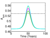
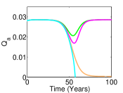
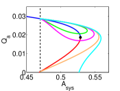
Figure 1 demonstrates the general effect, described for general systems in Section 2. The specific graphs have been computed for Zickfeld’s model for the Indian summer monsoon, a model with two time-dependent variables depending on the planetary albedo $A_{\mathrm{sys}}$ as a parameter, given in Section 3. The current planetary albedo is estimated as $A_{\mathrm{sys}}^{\infty}=0.47$ [13], where the monsoon is at a stable equilibrium with specific humidity $Q_{a}=0.03$. The tipping threshold for the shutdown of the monsoon is at $A_{\mathrm{sys}}^{b}\approx 0.53$ according to our simple model (dashed line in Figure 1(a)). For sufficiently slow monotone increases of the albedo $A_{\mathrm{sys}}$, the value $A_{\mathrm{sys}}^{b}$ is the tipping point, where in the model the monsoon shuts down. However, Figure 1(a) shows four scenarios for time profiles of the albedo, $A_{\mathrm{sys}}(t)$, where it temporarily crosses the tipping threshold $A_{\mathrm{sys}}^{b}$ but then returns back to its present day value $A_{\mathrm{sys}}^{\infty}$. Whether the monsoon shuts down depends on how far the albedo exceeds the tipping threshold maximally (the exceedance amplitude $R=\max A_{\mathrm{sys}}(t)-A_{\mathrm{sys}}^{b}$), and for how long (the exceedance time $t_{e}$), for each of these scenarios. Our general deterministic result applies for the case that the change of the albedo is slow compared to the internal time scales of the monsoon model, such that we may introduce a small parameter $\epsilon$ expressing this ratio of time scales. The criterion whether the monsoon avoids shutdown depends only on the parameters $R$ and $t_{e}$ of the albedo time profile and one system dependent quantity $d^{b}$ for small $\epsilon$. To avoid shutdown the exceedance amplitude $R$ has to be of order $\epsilon$ and

$$d^{b}\,R\,t_{e}^{2} \leq 16+O(\epsilon)\mbox{.}$$ (1)

Criterion (1) is general for scenarios when one temporarily crosses a critical threshold (mathematically a fold bifurcation), the parameter time profile can be approximated by a parabola close to the threshold, and the ratio $\epsilon$ of parameter drift speed to internal time scales is sufficiently small.

The consequences of our general result are shown in Figures 1(b) and 1(c). One of the time-dependent variables in the monsoon model, the specific humidity $Q_{a}(t)$, experiences a temporary drop in the first two scenarios, which meet criterion (1) (green: $R=0.01$, $t_{e}=8$, and pink: $R=0.02$, $t_{e}=11$). In contrast, $Q_{a}(t)$ drops far below its stable equilibrium value for the fourth scenario, which does not satisfy (1) (bright blue: $R=0.03$, $t_{e}=13.3$). Whilst the third scenario shows the solution for $Q_{a}(t)$ at the boundary of criterion (1) (light brown: $R\approx 0.027$, $t_{e}=12.7$). Figure 1(c) shows how albedo $A_{\mathrm{sys}}(t)$ and specific humidity $Q_{a}(t)$ change in combination. For the scenarios without tipping the trajectories form closed curves returning to their starting (present day) equilibrium values, while in the tipping scenario the trajectory escapes from the region where the model is valid. Figure 1(c) also contains the underlying equilibria for fixed albedo $A_{\mathrm{sys}}$. The stable equilibrium is blue, above $Q_{a}=0.02$, meeting the unstable equilibrium (red) in the point that would be the tipping point for fixed albedo (black dot at $A_{\mathrm{sys}}\approx 0.53$, $Q_{a}\approx 0.02$). The trajectory on the boundary established by equality in (1) connects the stable and the unstable equilibrium at the present day albedo value $0.47$ (light brown in Figure 1(c)). We may also formulate a criterion equivalent to (1) which depends on the acceleration $\ddot{A}_{\mathrm{sys}}(t)$ of the planetary albedo at its maximum. This is provided by equation (10).

Value and estimates of proportionality factor $d^{b}$

The system dependent proportionality factor $d^{b}$ depends on the decay rate -$\lambda(A_{\mathrm{sys}})$ toward the stable equilibrium for fixed albedo $A_{\mathrm{sys}}$ just below the critical threshold $A_{\mathrm{sys}}^{b}$. In the ratio

$$d(A_{\mathrm{sys}})=\frac{[-\lambda(A_{\mathrm{sys}})]^{2}}{A_{\mathrm{sys}}^{b}-A_{\mathrm{sys}}}$$ (2)

the decay rate $-\lambda(A_{\mathrm{sys}})$ is the negative of the leading eigenvalue $\lambda(A_{\mathrm{sys}})$ of the linearization of the system at the stable equilibrium, which is zero for $A_{\mathrm{sys}}=A_{\mathrm{sys}}^{b}$. Thus, both, numerator and denominator in (2) converge to $0$ as $A_{\mathrm{sys}}$ approaches its critical threshold $A_{\mathrm{sys}}^{b}$ from below. However, $d(A_{\mathrm{sys}})$ has a well defined limit from the left, defining $d^{b}$: $d(A_{\mathrm{sys}})\to d^{b}$ as $A_{\mathrm{sys}}\to A_{\mathrm{sys}}^{b}$ from below.

In real-world applications there is often no direct access to an underlying model. Instead, only time series output data, disturbed by random fluctuations, may be available, such as proxies for the temperature and $CO_{2}$ [20] in palaeo-climate records. For a constant parameter $A_{\mathrm{sys}}^{c}<A_{\mathrm{sys}}^{b}$ and close to the stable equilibrium, the system, when subjected to small white-noise disturbances, acts like a linear Ornstein-Uhlenbeck process where the decay rate $-\lambda$ is approximately related to the time-$\Delta t$ autocorrelation $a$ via [21]

$${\color[rgb]{0,0,0}-\lambda(A_{\mathrm{sys}}^{c})}\approx\dfrac{1-a}{\Delta t}\mbox{.}$$

Thus, we may estimate the quantity $d(A_{\mathrm{sys}}^{c})$ for some fixed $A_{\mathrm{sys}}^{c}<A_{\mathrm{sys}}^{b}$ (but still $A_{\mathrm{sys}}^{c}\approx A_{\mathrm{sys}}^{b}$) by $d(A_{\mathrm{sys}}^{c})\approx(1-a)^{2}/[(\Delta t)^{2}(A_{\mathrm{sys}}^{b}-A_{\mathrm{sys}}^{c})]$, where $a$ is the time $\Delta t$ autocorrelation of an output time series (e.g., specific humidity $Q_{a}(t)$ or atmospheric temperature $T_{a}(t)$), observed for the fixed parameter $A_{\mathrm{sys}}^{c}$. Then we use this as an approximation for $d^{b}$ since $d(A_{\mathrm{sys}}^{c})$ approaches $d^{b}$ for $A_{\mathrm{sys}}^{c}\to A_{\mathrm{sys}}^{b}$. Inserting this approximation into (1), we obtain a simplified dimensionless criterion that a parameter change policy $A_{\mathrm{sys}}(t)$ avoids tipping if

$$\frac{(1-a)^{2}}{A_{\mathrm{sys}}^{b}-A_{\mathrm{sys}}^{c}}\left[\max_{t}A_{\mathrm{sys}}(t)-A_{\mathrm{sys}}^{b}\right]N_{e}^{2}\leq 16+O(\epsilon)\mbox{.}$$

In this criterion the autocorrelation was measured at $A_{\mathrm{sys}}^{c}$ (for example, present-day value $A_{\mathrm{sys}}^{\infty}$), and $N_{e}$ is the number of time units above threshold $A_{\mathrm{sys}}^{b}$, using the same time unit as for measuring the autocorrelation $a$ (so $N_{e}=t_{e}/\Delta t$). The autocorrelation $a$ and the variance of output time series are expected to increase when the parameter $A_{\mathrm{sys}}^{c}$ approaches the tipping threshold $A_{\mathrm{sys}}^{b}$ from below. This has motivated extensive studies in field data (such as palaeo climate records or lake sediments), investigating whether autocorrelation and variance act as early-warning indicators of tipping [22, 23, 16, 24]. See also Ritchie and Sieber [25] for a study on the behavior of early-warning indicators when the parameter is changed at higher speed, causing rate-induced tipping, and Dakos et al. [23] for methods on calculating autocorrelation and variance.

Probabilistic result

(see Section 4) If the system is subject to small white-noise disturbances of variance $2D$, tipping may occur with positive probability even if the albedo time profile $A_{\mathrm{sys}}(t)$ never exceeds the critical threshold $A_{\mathrm{sys}}^{b}$ (that is, $R<0$). Thus, the exceedance time $t_{e}(A_{\mathrm{sys}}^{\mathrm{th}})$, measuring the time the parameter $A_{\mathrm{sys}}(t)$ spends above a fixed threshold value $A_{\mathrm{sys}}^{\mathrm{th}}<A_{\mathrm{sys}}^{b}$ becomes a relevant parameter. We find that the level curves of constant probability of escape follow the inverse square in parts of the parameter space if the time scale ratio $\epsilon$ and the noise variance have the relation $\epsilon\sim D^{2/3}$. If $\epsilon\gg D^{2/3}$, the probabilistic result reverts to the deterministic case, while for $\epsilon\ll D^{2/3}$ the tipping probability is close to $1$. We provide a numerically computed graph of escape probabilities that is accurate in the limit $\epsilon\to 0$ and $D^{2/3}\sim\epsilon$ (fitting coefficients are in the Supplementary Material). We also provide approximations for the escape probabilities in several limiting cases of the provided graph.

In Section 5 we will illustrate the escape probability estimates for the monsoon model with additive noise. The Supplementary Material provides detailed expressions for the projection of a general $n$-dimensional system onto a scalar ODE, and for the approximations of the escape probability in the presence of noise.

2 Critical distance and time over threshold before tipping

Assumptions on the dynamical system

We consider an $n$-dimensional system of ordinary differential equations (ODEs) with a scalar output $y_{o}$

$$\dot{\mathbf{y}}(t) =f(\mathbf{y}(t),q(t))\mbox{,} \mathbf{y}(t) \in\mathbb{R}^{n}\mbox{,}\,q(t)\in\mathbb{R}$$ (3)

$$y_{o}(t) =\mathbf{w}^{T}\mathbf{y}(t)\mbox{,} y_{o}(t) \in\mathbb{R}\mbox{,}\,\mathbf{w}\in\mathbb{R}^{n}\mbox{.}$$

that has a fold (saddle-node) bifurcation for constant $q$ at $(\mathbf{y},q)=(\mathbf{y}^{b},q^{b})$. Specifically, we make the following assumptions ((S1)-(S4) define the fold bifurcation [26]):

1. the linearization $A_{1}=\partial_{1}f(\mathbf{y}^{b},q^{b})$ is singular and has a single right nullvector $\mathbf{v}_{0}$ and a single left nullvector $\mathbf{w}_{0}$ ($A_{1}\mathbf{v}_{0}=0$, $\mathbf{w}_{0}^{T}A_{1}=0$), scaled such that $\mathbf{w}_{0}^{T}\mathbf{v}_{0}=1$;

2. all other eigenvalues of $A_{1}$ have negative real part: one of the branches of the fold is stable;

3. $a_{0}:=\mathbf{w}_{0}^{T}\partial_{2}f(\mathbf{y}^{b},q^{b})\neq 0$: changing the parameter $q$ crosses the fold transversally;

4. $\kappa:=\frac{1}{2a_{0}}\mathbf{w}_{0}^{T}\partial_{1}^{2}f(\mathbf{y}^{b},q^{b})\mathbf{v}_{0}^{2}\neq 0$: only one node and one saddle collide in the fold;

5. $\mathbf{w}^{T}\mathbf{v}_{0}\neq 0$: one can observe the dynamics in the critical direction $\mathbf{v}_{0}$ through the output $y_{o}$; thus we scale $\mathbf{v}_{0}$ such that $\mathbf{w}^{T}\mathbf{v}_{0}=1$.

We use the convention that $\partial_{1}^{k}f(\mathbf{y},q)$ and $\partial_{2}^{k}f(\mathbf{y},q)$ refer to the $k$th order partial derivatives of $f$ with respect to $\mathbf{y}$ and $q$ respectively. Without loss of generality we assume that the stable equilibrium involved in the fold exists for $q<q^{b}$ and the stable equilibrium has output $y_{o}<y_{o}^{b}:=\mathbf{w}^{T}\mathbf{y}^{b}$, such that the signs of $a_{0}$ and $\kappa$ are positive:

$$a_{0} >0\mbox{,} \kappa >0\mbox{.}$$

Otherwise, we may change the sign of the considered output projection $\mathbf{w}$ or parameter $q$.

Assumptions on the forcing

We assume that the dependence of the parameter on time, $q(t)$, is slow, differentiable sufficiently often, and that $q(t)$ reaches a maximum, which we can assume without loss of generality to be at time $t=0$. Thus, $q(t)$ can be split into a constant part (equal to $q^{\max}$) and a time-dependent part $q_{h}$ with a time dependence of the form $\epsilon t$ and a small parameter $\epsilon$: $q(t)=q^{\max}+q_{h}(\epsilon t)$, where, by our assumptions, $q_{h}(0)=\dot{q}_{h}(0)=0$. The slowness of the parameter change implies that for $q^{\max}>q^{b}$ the system will tip for sufficiently small $\epsilon$, unless the overshoot of the forcing beyond the bifurcation value $q^{b}$, the maximal exceedance $q^{\max}-q^{b}$, is small. Thus, we may introduce a rescaled measure $R_{0}$ of the maximal exceedance such that $q^{\max}=q^{b}+\epsilon R_{0}$ (the analysis below will show that for small $\epsilon$ the boundary for tipping occurs for $R_{0}$ of order $1$). Furthermore, we assume that the parameter forcing $q(t)$ reaches a regular maximum at time $t=0$, such that $R_{2}:=-\frac{1}{2}q_{h}^{\prime\prime}(0)>0$ (using $(\cdot)^{\prime}$ to indicate the derivative of a single-argument function with respect to its argument). In summary, we assume that the parameter forcing is of the form

$$q(t)=q^{b}+\epsilon R_{0}+q_{h}(\epsilon t)\mbox{,}$$ (4)

where $\epsilon$ is small and

1. $q_{h}(0)=0$: the parameter $q(t)$ reaches the value $q^{\max}=q^{b}+\epsilon R_{0}$ (without loss of generality) at time $0$;

2. $q_{h}^{\prime}(0)=0$: the value $q^{\max}$ is a critical point of the parameter dependence, making the encounter of the fold at $q^{b}$ non-transversal for $R_{0}=0$;

3. $R_{2}:=-\frac{1}{2}q_{h}^{\prime\prime}(0)>0$: the parameter forcing has a regular maximum at time $t=0$.

Assumption P2 implies that we are studying the vicinity of a degeneracy. Commonly, one assumes that the crossing of the bifurcation is transversal (that is, $q_{h}^{\prime}(0)>0$, making P3 unnecessary) [27, 28, 29, 30, 31]. The case $q_{h}^{\prime}(0)>0$ is called a slow (in comparison to the response time of the system) transversal passage through a fold bifurcation. For the transversal case it has been shown [14, 15] that solutions track the stable equilibrium branch for $t<0$ at a distance of order $\epsilon^{1/3}$ and that solutions gain distance of order $1$ from the equilibrium branch with a delay of order $\epsilon^{2/3}$ such that $y(t)-y^{b}\sim O(1)$ for times $t\sim\epsilon^{2/3}$. Li et al. [32] determine the precise time at which $\mathbf{y}$ reaches order $1$, corresponding to an escape to infinity after rescaling, calling it the “point of no return” for a linear forcing. The textbook by Berglund and Gentz [14] also derives asymptotic probabilities and escape times for tipping in the presence of white noise in the small-$\epsilon$-small-variance regime.

The assumptions imply that we have for fixed $q<q^{b}$ a branch of stable equilibria $(\mathbf{y}^{s}(q),q)$ and a branch of unstable equilibria $(\mathbf{y}^{u}(q),q)$ of (3) (all satisfying $0=f(\mathbf{y}^{s,u}(q),q)$), which meet in the fold at parameter $q^{b}$ in point $\mathbf{y}^{b}$. We expect a solution $\mathbf{y}(t)$, starting from close to $\mathbf{y}^{s}(q(t_{0}))$ with $t_{0}<0$ to follow the stable branch closely for sufficiently small $\epsilon$ until we reach the vicinity of $\mathbf{y}^{b}$ at time $t<0$ of order $1$.

In the vicinity of the fold $(\mathbf{y}^{b},q^{b})$, we may zoom in and speed up time:

$$x :=\epsilon^{-1/2}(y_{\color[rgb]{0,0,0}o}-y_{o}^{b})=\epsilon^{-1/2}\mathbf{w}^{T}(\mathbf{y}-\mathbf{y}^{b})\mbox{,}$$ (5)

$$t_{\mathrm{new}} :=\epsilon^{1/2}t_{\mathrm{old}}\mbox{.}$$

Then combined with the expansion for $q(t)$, equation (4), $x$ satisfies the scalar differential equation [33]

$$\dot{x}=a_{0} \left(R_{0}-R_{2}t^{2}+\kappa x^{2}\right)+O(\epsilon^{1/2})\mbox{.}$$ (6)

If $R_{0}$ is sufficiently large, the trajectory $x(t)$ will grow to large values for positive $t$ and small $\epsilon$ (since $a_{0}>0$). Thus, $\mathbf{y}(t)$ will leave the neighborhood of the branches of equilibria (corresponding to tipping).

The system quantities $a_{0}$ and $\kappa$ can be estimated from observations of the output $x$ for fixed parameter $q$ (thus, $R_{2}=0$): $2\kappa$ is the curvature of the equilibrium curve as observed through $x$ in $x=0$ (but also in the $(y_{o},q)$ plane in $(y_{o}^{b},q^{b})$). The decay rate of (6) at $R_{2}=0$ and fixed $R_{0}<0$ toward the stable equilibrium equals $2a_{0}\sqrt{-R_{0}\kappa}$ (recall that $\kappa>0$). Note that this is the decay rate for the sped up time $t_{\mathrm{new}}$.

For small $\epsilon$, the scalar equation (6) has solutions that are asymptotically $x(t)\sim-|t|\sqrt{R_{2}/\kappa}$ for large $t$ if (see [10])

$$R_{0}<\frac{1}{a_{0}}\sqrt{\frac{R_{2}}{\kappa}}+o(1)\mbox{.}$$ (7)

(The term $o(1)$ stands for terms that go to $0$ for $\epsilon\to 0$.) For $\kappa a_{0}^{2}R_{0}^{2}=R_{2}$ and $\epsilon=0$ the orbit $x(t)=t\sqrt{R_{2}/\kappa}$ is the only solution existing for all time (connecting $x\sim t$ at $-\infty$ and $+\infty$). In the original coordinates this gives a first-order expansion for the condition relating the maximum value of $q(t)$ and its acceleration at the maximum to each other. By assumptions P1–P3 the maximum of $q(t)$ is attained at $t=0$, $\max_{t}q(t)=q^{b}+\epsilon R_{0}$, and the acceleration of $q$ at $0$ equals $\ddot{q}(0)=\frac{\mathrm{d}^{2}}{\mathrm{d}t^{2}}q_{h}(\epsilon t)|_{t=0}=-2\epsilon^{2}R_{2}$ (by expansion (4) of $q$). Expressed using $q(0)$ and $\ddot{q}(0)$, criterion (7) for avoiding tipping (including the small perturbation $\epsilon$ again) reads

$$q(0)<q_{\mathrm{crit}}(\epsilon):=q^{b}+\frac{1}{a_{0}}\sqrt{-\frac{\ddot{q}(0)}{2\kappa}}+o(\epsilon)\mbox{.}$$ (8)

The first term added to $q^{b}$ is of order $\epsilon$ since $\ddot{q}(0)=\epsilon^{2}q_{h}^{\prime\prime}(0)=-{\color[rgb]{0,0,0}2}\epsilon^{2}R_{2}+o(\epsilon^{2})$. The combination of the quantities $a_{0}$ and $\kappa$, needed for (8), $1/(a_{0}\sqrt{\smash[b]{2\kappa}})$, may be found via the left limit

$$d^{b}:=\lim_{q\nearrow q^{b}}\frac{[-\lambda(q)]^{2}}{q^{b}-q}\mbox{,}$$ (9)

where $\lambda(q)$ is the leading eigenvalue of the linearization of underlying system (3) toward the stable equilibrium $y^{s}(q)$ (or, equivalently, the negative of the decay rate toward $y^{s}(q)$) in the original time-scale $t_{\mathrm{old}}$ and spatial scale $\mathbf{y}$. Then $d^{b}=4a_{0}^{2}\kappa$, such that the acceleration criterion (8) for avoiding tipping becomes

$$q(0)<q_{\mathrm{crit}}(\epsilon)=q^{b}+\sqrt{-\frac{2\ddot{q}(0)}{d^{b}}}+o(\epsilon)\mbox{,}$$ (10)

where both, $d^{b}$ and $\ddot{q}(0)$, are computed in the original time and space scale. Thus, to establish the critical permissible distance $\max_{t}q(t)-q^{b}$ over the threshold before tipping, we need some estimate of the attraction rate toward the stable equilibria near the fold. This decay rate can, for example, be estimated through the autocorrelation in the output time series $y_{o}(t)$ when the system is subject to fluctuations [22, 23, 20, 34].

Furthermore, for every forcing $q(t)$ exceeding the bifurcation value $q^{b}$ ($q(0)>q^{b}$) we may, as an alternative to $\ddot{q}(0)$, consider the exceedance time $t_{e}$, the time that the parameter forcing $q(t)$ spends beyond the fold bifurcation value $q^{b}$. In the original time scale, expanding the parameter forcing $q(t)$ with respect to $t$:

$$q(t)=q(0)+\frac{1}{2}\ddot{q}(0)t^{2}+O(\epsilon t)^{3},$$

and establishing the times $t_{\pm}$ at which the parameter forcing crosses $q^{b}$

$$t_{\pm}=\pm\sqrt{\dfrac{2(q^{b}-q(0))}{\ddot{q}(0)}}+O(1),$$

gives the relationship between $t_{e}$ and the other forcing parameters $q(0)$ and $\ddot{q}(0)$ as approximately

$$t_{e} ={\color[rgb]{0,0,0}t_{+}-t_{-}=}\sqrt{\frac{8(q^{b}-q(0))}{\ddot{q}(0)}}+O(1)=\sqrt{\frac{4R_{0}}{\epsilon R_{2}}}+O(1)\mbox{.}$$ (11)

As the second expression makes clear, the exceedance time $t_{e}$ is large (of order $\epsilon^{-1/2}$), even when the amplitude of the exceedance $\epsilon R_{0}+O(\epsilon^{2})$ is small. We can then insert relation (11) into (10) to eliminate $\ddot{q}(0)$ and establish the inverse-square law for maximal exceedance amplitude $q(0)-q^{b}$ and time of exceedance $t_{e}$ that avoids tipping (recall that $q(0)=\max_{t}q(t)=q^{\max}$ and $d^{b}$ is given by (9)):

$$d^{b}\left[q^{\max}-q^{b}\right]t_{e}^{2}\leq 16\mbox{,\quad or,\quad}a_{0}^{2}\kappa\left[q^{\max}-q^{b}\right]t_{e}^{2}\leq 4\mbox{.}$$ (12)

In applications the parameter forcing is typically not given in the form of an expansion such as (4), but rather as a function of time $q(t)$. The quantities $d^{b}$, $q^{\max}-q^{b}$ and $t_{e}$ can be computed or estimated without explicitly introducing $\epsilon$. Then the above inequality is a valid criterion for the tipping threshold if $q^{\max}-q^{b}$ is small in modulus, while $t_{e}$ is large and the forcing is approximately parabolic in $[-t_{e},t_{e}]$.

3 Indian summer monsoon model

We illustrate the general deterministic criterion using a conceptual model for one of the recognized policy-relevant tipping elements in the Climate System, the Indian summer monsoon [1, 35]. The Indian economy and agriculture is heavily reliant on the Indian summer monsoon [36] as it provides the main source of water for India [37]. In the second half of the 20th century, summer rainfall has decreased leading to an increasing frequency of droughts [38], reducing rice harvests [39]. In particular, in 2002 India experienced a major drought with a seasonal rain deficit of $21.5\%$ [36], seeing an increase in suicides amongst farmers and an estimated cost of $340$ million dollars to the Indian government for drought relief programs [37]. Meehl et al. [40] connect these observations of decreased rainfall and increased droughts to an already present disruption of the monsoon.

We study a model for the Indian summer monsoon [13], which contains the key driving force of the monsoon, a moisture-advection feedback loop [12]. In the summer months the land is warmer than the ocean. This temperature difference generates winds coming off the Indian Ocean onto the land. The winds carry moisture from the ocean which is deposited over the land in the form of precipitation. This process releases latent heat, meaning that the temperature over land increases. A larger temperature difference causes stronger winds carrying more moisture and hence the positive feedback loop is formed.

We use a conceptual model proposed by Zickfeld [11] and make further simplifications, though retaining the key mechanism of the monsoon, the positive feedback loop described above. The model has two time-dependent variables, the specific humidity $Q_{a}$ and the atmospheric temperature $T_{a}$, are described by the following ODEs:

$$\dot{Q}_{a} =\dfrac{E-P+A_{v}}{\beta I_{q}},$$ (13)

$$\dot{T}_{a} =\dfrac{\mathcal{L}(P-E)-F_{\uparrow}^{LW,TA}+F_{\downarrow}^{SL,TA}(1-A_{\mathrm{sys}})+A_{T}}{\beta I_{T}}$$ (14)

where the terms on the right-hand side are grouped as follows:

• Evaporation $E$ (mm$/$s): Proportional to the temperature difference between the land $T_{a}$ and the Indian Ocean $T_{oc}$ and to the difference between saturated humidity $Q_{\mathrm{sat}}$ and specific humidity $Q_{a}$

  $$E:=E(Q_{a},T_{a})=C_{E}(T_{a}-T_{oc})(Q_{\mathrm{sat}}-Q_{a}).$$

• Precipitation $P$ (mm$/$s): Proportional to the specific humidity

  $$P:=P(Q_{a})=C_{P}Q_{a}.$$

• Moisture advection $A_{v}$ (mm$/$s): Winds driven by the temperature difference between the land and ocean bring moisture from the ocean over land proportional to the humidity over the ocean $Q_{oc}$. Winds are reversed above a given height taking moisture away proportional to the humidity over land $Q_{a}$

  $$A_{v}:=A_{v}(Q_{a},T_{a})=(T_{a}-T_{oc})(C_{mo}Q_{oc}-C_{ml}Q_{a}).$$

• Outgoing long-wave radiation $F_{\uparrow}^{LW,TA}$ (kg$/$s³): Proportional to the temperature of the land

  $$F_{\uparrow}^{LW,TA}:=F_{\uparrow}^{LW,TA}(T_{a})=C_{L1}T_{a}+C_{L2}.$$

• Incoming short-wave radiation $F_{\downarrow}^{SL,TA}$ (kg$/$s³): Fraction of incoming solar radiation not reflected, proportional to $1-A_{\mathrm{sys}}$, where $A_{\mathrm{sys}}$ is the system planetary albedo.

• Heat advection $A_{T}$ (kg$/$s³): Winds driven by the temperature difference between the land and ocean bring cool air at a prescribed low altitude proportional to the potential temperature $\theta_{\mathrm{oc}}$ above the ocean ($\theta_{oc}$ is fixed). Reversed winds at a prescribed high altitude $z_{h}$ take warm air away proportional to the potential temperature above the land $\theta_{a}(Q_{a},T_{a})$. The potential temperature at the prescribed height $z_{h}$ is given by $\theta_{a}=T_{a}-(\Gamma(T_{a},Q_{a})-\Gamma_{a})z_{h}$ where $\Gamma=\Gamma_{0}+\Gamma_{1}(T_{a}-T_{0})(1-\Gamma_{2}Q_{a}^{2})$ (with a reference temperature $T_{0}$) is the atmospheric lapse rate and $\Gamma_{a}$ is the adiabatic lapse rate

  $$A_{T}:=A_{T}(Q_{a},T_{a})=C_{H}(T_{a}-T_{oc})(\theta_{oc}-\theta_{a}(Q_{a},T_{a})).$$

The remaining terms are all constants. The constant ${\cal L}$ is the latent heat, and $\beta$ converts from seconds to decades (the unit of time $t$ is decades). Appendix C, Table 1 lists all parameters and their values and units.

Zickfeld et al. [13] identified two quantities that are influenced by human activities or subject to natural variation and affect the stability of the monsoon. In the model either an increase of the planetary albedo $A_{\mathrm{sys}}$ or a decrease in the $CO_{2}$ concentration from present day values can potentially lead to a “shutdown” of the Indian monsoon. We will focus our analysis on the possibility of an increase in the planetary albedo.

The planetary albedo represents the ratio of reflected to incoming solar radiation and can be influenced by atmospheric aerosols and land-cover conversion [13]. In particular, the atmospheric brown cloud haze hanging over the Indian subcontinent has been considered responsible for the disruption of the monsoon with some future projections suggesting the drought frequency could double within a decade [38]. This cloud haze is predominately made up of black carbon aerosols emanating from fossil fuel combustion and biomass burning, which both absorb and reflect (thus, increasing planetary albedo) incoming radiation [40]. Knopf et al. [41] have previously performed a multi-parameter uncertainty analysis for the original Zickfeld model, which models the planetary albedo as a function of the surface albedo. They concluded that if the model is reliable the bifurcation point for the surface albedo is sufficiently far from present day values such that this point cannot be reached in the near future. However, brown haze is typically poorly captured by the functional dependency assumed in the models [1]. Thus, the pollution-driven changes such as brown haze may place the monsoon system closer to its bifurcation point than concluded by Knopf et al. [41]. On a positive note this pollution is a regional problem, so does not require any world-wide agreement [37] and therefore reversion of tipping by rapid action may be politically more feasible [35]. Note that, despite its name the planetary albedo is a regional property for the Indian subcontinent in this model.

Zickfeld et al. [13] states that the present day value of the planetary albedo is $A_{\mathrm{sys}}^{\infty}=0.47$. This is comparable with radiative transfer model output data for the period 1984-1997, which suggests an averaged summer value of around $0.45$ for India [42]. For fixed $A_{\mathrm{sys}}$ system (13)–(14) has a fold (saddle-node) bifurcation at $A_{\mathrm{sys}}^{b}\approx 0.53$, as shown as a black dot in the $(A_{\mathrm{sys}},Q_{a})$-plane in Figure 1(c). A slow increase of the planetary albedo linearly beyond the fold will cause tipping in the monsoon model, a sudden drop in the specific humidity would be observed. Equation (14) highlights how increasing the planetary albedo affects the positive feedback loop outlined above. As the albedo increases, the change in temperature over land decreases, meaning a smaller temperature difference between the land and ocean and hence weaker winds are formed. We will use criterion (12) to estimate how long the planetary albedo may exceed the fold bifurcation parameter value $A_{\mathrm{sys}}^{b}$ without causing a tipping of the Indian summer monsoon in the model. While the general tipping criterion (12) could in principle be used to guide policy, model (13), (14) is only conceptual such that the precise figures for $A_{\mathrm{sys}}(t)$ serve as an illustration of the general result, rather than as policy guidelines. We assume a change of planetary albedo as a temporary increase from a background value $A_{\mathrm{sys}}^{\infty}$, namely

$$A_{\mathrm{sys}}(t)=A_{\mathrm{sys}}^{\infty}+\frac{R+A_{\mathrm{sys}}^{b}-A_{\mathrm{sys}}^{\infty}}{\cosh(S(t_{\mathrm{end}}-2t))^{2}}$$ (15)

for a time interval $[0,t_{\mathrm{end}}]$. The parameters $R$ and $S$ correspond to the amount of overshoot and the speed of forcing respectively. They are both small and of equal magnitude, such that we may introduce rescaled parameters via

$$R =r_{1}\epsilon\mbox{,} S =s_{1}\epsilon\mbox{.}$$

Equation (15) describes an increase of the planetary albedo towards (and, if $R>0$, beyond) the fold bifurcation value $A_{\mathrm{sys}}^{b}$ before it returns to its present day (background) value $A_{\mathrm{sys}}^{\infty}$. Figure 1(a) in the introduction shows four example time profiles of planetary albedo forcing (15) for illustration. All four fix the speed of forcing $S=0.5$, and vary $R$, the difference between maximal albedo and its bifurcation value $A_{\mathrm{sys}}^{b}$. The exceedance $R$ of the maximal albedo beyond the fold bifurcation value $A_{\mathrm{sys}}^{b}$ (indicated by the horizontal dashed line) and the time $t_{e}$ the albedo $A_{\mathrm{sys}}(t)$ spends above $A_{\mathrm{sys}}^{b}$ are determined by $S$ and $R$ via

$$t_{e}={\color[rgb]{0,0,0}\frac{1}{S}}\sqrt{\frac{R}{A_{\mathrm{sys}}^{b}-A_{\mathrm{sys}}^{\infty}}}+O(R^{3/2}/{\color[rgb]{0,0,0}S})\mbox{.}$$

Specifically expressing the exceedance time in quantities of order 1 and $\epsilon$

$$t_{e}={\color[rgb]{0,0,0}\frac{1}{\sqrt{\epsilon}}\frac{1}{s_{1}}}\sqrt{\frac{r_{1}}{A_{\mathrm{sys}}^{b}-A_{\mathrm{sys}}^{\infty}}}+O(\epsilon^{1/2})\mbox{,}$$

we can see the exceedance time is large (of order $\epsilon^{-1/2}$), consistent with equation (11). The error is of order $\epsilon^{1/2}$ (smaller than the error of order 1 in (11)) due to the even symmetry of the forcing $A_{\mathrm{sys}}(-t)=A_{\mathrm{sys}}(t)$.

In addition to the illustrative curves shown in Figure 1, we compare the asymptotic approximation (1) to the numerically computed critical curve separating a “safe” area (monsoon retained) from the “unsafe” area, where escape toward shutdown occurs, in the two-parameter plane. We choose as forcing parameters the peak exceedance beyond the fold $R$, and exceedance time $t_{e}$.

The critical parameters, for which the exact (numerically computed) connecting orbit to the saddle occurs, are shown as a blue solid curve in Figure 2. As discussed in Section 2, the critical amount by which the planetary albedo exceeds the fold value $A_{\mathrm{sys}}^{b}$ is approximately inversely proportional to the square of the time the planetary albedo stays above $A_{\mathrm{sys}}^{b}$. For example, if the planetary albedo increases just above the bifurcation ($R=0.005$) then the system can spend a long time ($\sim 30$ years) above the bifurcation value without shutting down the monsoon. However, for a higher maximum of $A_{\mathrm{sys}}$ ($R=0.02$ above the bifurcation value) the system can maintain the monsoon only if the exceedance time $t_{e}$ is shorter ($\sim 15$ years).

Figure 2: Tipping region in the two parameter plane $R=\max_{t}A_{\mathrm{sys}}(t)-A_{\mathrm{sys}}^{b}$ (Peak distance over fold (saddle-node)) and $t_{e}$ (time above fold). Safe region and escape region separated by the numerically calculated critical curve (blue solid). The red dashed curve provides an approximation of the critical curve obtained from equation (12), where $d^{b}=318.36$ per decades².

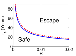
The parameter values satisfying the theoretical inequality (1) (valid for the limit $\epsilon\to 0$) are below the red dashed curve in Figure 2. The curve gives a good approximation to the numerically calculated critical curve. The approximation is best for small critical $R$ (peak distance over fold) because then the system spends most time in the region of the phase space where the second-order expansion of the right-hand side in the fold and of the forcing in its maximum are valid (both of these were assumed in the derivation of inequality (12), and, thus, (1)).

4 Probability of tipping under the influence of noise

In this section we study the probability of escape when the system is, in addition to its parameter drift, subject to random disturbances, which we model by adding white noise to (3):

$$\mathrm{d}\mathbf{y}(t)=f(\mathbf{y}(t),q(t))\mathrm{d}t+\Sigma\mathrm{d}W_{t}\mbox{,}$$ (16)

where $\Sigma$ is a $n\times\ell$ matrix of noise amplitudes, and $\mathrm{d}W_{t}$ are the increments of $\ell$ Wiener processes. We again consider a changing parameter $q(t)$ satisfying conditions P1–P3 and expansion (4), touching a fold $(\mathbf{y}^{b},q^{b})$ of the deterministic part satisfying conditions S1–S5. Similar to the analysis of the deterministic case in Section 2, the dynamics of (16) can be studied near the fold $(\mathbf{y}^{b},q^{b})$ by projecting it onto its center direction using the right ($\mathbf{v}_{0}$) and left ($\mathbf{w}_{0}$) eigenvectors of $\partial_{1}f(\mathbf{y}^{b},q^{b})$. We focus on the case where after this projection the noise amplitude is sufficiently small (say, of order $\sigma\ll 1$) such that escape is unlikely at times when the parameter forcing $q(t)$ is away from its maximum $q^{\max}$ (for $|t|\gg 1/\epsilon$). The behavior of the noise-disturbed system depends on the asymptotic relation between small noise variance of order $\sigma^{2}$ and small parameter drift speed $\epsilon$.

Two sections in the Supplementary Material derive in detail that for $\sigma^{2}\ll\epsilon^{3/2}$ the probabilistic case reverts to the deterministic case studied in Section 2, while for $\sigma^{2}\gg\epsilon^{3/2}$ the probability of tipping will approach $1$ for $\sigma\to 0$ (and, hence, $\epsilon\to 0$). Thus, for a non-trivial limit of small noise variance $\sigma^{2}$ and parameter drift speed $\epsilon$, we require a scaling of $\sigma^{2}=\epsilon^{3/2}$. The argument in the Supplementary Material follows the textbook of Berglund and Gentz [14], exploiting that close to the fold the decay rate in the center direction $\mathbf{v}_{0}$ is much smaller than the decay rates in the stable directions $\mathbf{y}_{s}$ (defined by $\mathbf{w}_{0}^{T}\mathbf{y}_{s}=0$), such that the coupling between stable and center directions is small. One underlying assumption is that the scaled projection $\sigma^{-1}\mathbf{w}_{0}^{T}\Sigma$ of the noise onto the center direction is of order $1$ (that is, it is not much smaller than the scaled projection $\sigma^{-1}[I-v_{0}\mathbf{w}_{0}^{T}]\Sigma$ onto the stable directions).

Consequently, the projection of $\Sigma$ by $\mathbf{w}$ onto the scalar output, after the rescaling (5) to the zoomed-in output $x=\epsilon^{1/2}\mathbf{w}^{T}(\mathbf{y}-\mathbf{y}^{b})$ and sped up time $\epsilon^{-1/2}t$ (see (5)), has the variance ($\Delta=\Sigma\Sigma^{T}$)

$$2D:=2\epsilon^{-3/2}\mathbf{w}_{0}^{T}\Delta\mathbf{w}_{0}\mbox{,}$$ (17)

which is of order $1$.

Furthermore, if the the matrix of noise amplitudes $\Sigma$ in (16) depends on the state $\mathbf{y}$, then after the rescaling (5) the dependence of $D$ on $x$ becomes weak, of order $\epsilon^{1/2}$, such that we neglect it to leading order.

In the limit for $\epsilon\to 0$, the projected equation (16) becomes the scalar stochastic differential equation (SDE)

$$\mathrm{d}x =a_{0}[R_{0}-R_{2}t^{2}+\kappa x^{2}]\mathrm{d}t+\sqrt{2D}\mathrm{d}W_{t}\mbox{}$$ (18)

(recall that $a_{0}>0$ and $\kappa>0$ without loss of generality), starting from $x(t_{0})\leq 0$ and $t_{0}<0$ (see Supplementary Material). By further rescaling $x$ and time and introducing correspondingly rescaled versions of the parameters $R_{0}$ and $R_{2}$,

$$x_{\mathrm{new}} =\frac{(a_{0}\kappa)^{1/3}}{D^{1/3}}x_{\mathrm{old}}\mbox{,} t_{\mathrm{new}} =D^{1/3}(a_{0}\kappa)^{2/3}t_{\mathrm{old}}\mbox{,} p_{0} =\frac{a_{0}^{2/3}R_{0}}{D^{2/3}\kappa^{1/3}}\mbox{,} p_{2} =\frac{R_{2}}{D^{4/3}\kappa^{5/3}a_{0}^{2/3}}\mbox{,}$$ (19)

we may simplify (18) to a SDE

$$\mathrm{d}x =[p_{0}-p_{2}t^{2}+x^{2}]\mathrm{d}t+\sqrt{2}\mathrm{d}W_{t}\mbox{}$$ (20)

with unit noise amplitude and nonlinear coefficient, and the two parameters $p_{0}\in\mathbb{R}$ and $p_{2}>0$. The lines $x=\sqrt{p_{2}}t$ for $t\ll-1$ and $x=-\sqrt{p_{2}}t$ for $t\gg 1$ are stable slow manifolds of the deterministic part of (20). Thus, the density of $x$ at some fixed large time $t=-T_{0}$ is nearly independent from the initial density for $t\ll-T_{0}$ (conditional on no escape occurring before $t=-T_{0}$). Thus, we can compute numerically the probability of escape by solving the Fokker-Planck equation (FPE) [43] for the density $u(x,t)$ of $x$

$$\partial_{t}u(x,t)=\partial_{x}^{2}u(x,t)-\partial_{x}[(p_{0}-p_{2}t^{2}+x^{2})u(x,t)]$$ (21)

with Dirichlet boundary conditions $u(x_{\mathrm{bd}},t)=u(-x_{\mathrm{bd}},t)=0$ from $t=-T_{0}$ to $t=+T_{0}$, starting from an arbitrary density concentrated in the region $\{x\leq 0\}$ and a sufficiently large $T_{0}$. The resulting escape probability $P_{\mathrm{esc}}(p_{0},p_{2})$ is then (approximately for large $T_{0}$ and large $x_{\mathrm{bd}}$) given by

$$P_{\mathrm{esc}}(p_{0},p_{2})=1-\int_{-x_{\mathrm{bd}}}^{x_{\mathrm{bd}}}u(x,T_{0})\mathrm{d}x\mbox{.}$$ (22)

The result (using chebfun [44]) is shown in Figure 3. Since in the probabilistic scenario, tipping is possible also for forcings $p(t)=p_{0}-p_{2}t^{2}$ that do not exceed the critical value $p_{0}^{b}=0$, it is useful to also consider other (especially lower) thresholds than $p_{0}^{b}$ (indicated by the white dashed line) for measuring exceedance amplitudes and times. In Figure 3 we choose $p_{0}^{\mathrm{th}}=-1$, and, hence, consider the parameter plane $(R^{(-1)},t_{e}^{(-1)})$ where

$$R^{(-1)} =p_{0}-p_{0}^{\mathrm{th}}\in[0,3]\mbox{,\quad and} t_{e}^{(-1)} =2\sqrt{(p_{0}-p_{0}^{\mathrm{th}})/p_{2}}\in[1,5]$$

are the maximal distance over the threshold $p_{0}^{\mathrm{th}}$ and the exceedance time spent above $p_{0}^{\mathrm{th}}$.

Figure 3: Probability of escape, $P_{\mathrm{esc}}$ of $x\to+\infty$ in (20) for parameter values $R^{(-1)}=p_{0}+1$ and $t_{e}^{(-1)}=2\sqrt{(p_{0}+1)/p_{2}}$ (exceedance amplitudes and times beyond the arbitrary threshold $p_{0}^{\mathrm{th}}=-1$). Parameters for FPE (21): domain $[-8,8]$, time interval $[-T_{0},T_{0}]$, initial density $N(x_{0},1)$ where $T_{0}=\sqrt{(x_{0}^{2}+p_{0})/p_{2}}$ and $x_{0}=-4$. White dashed line indicates the static fold bifurcation, black dashed curve shows the critical parameter values for deterministic tipping and the red solid curve indicates the boundary for validity of the mode approximation.

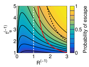
In the lower right corner of Figure 3, the level curves of equal probability align with the inverse-square law for deterministic tipping (black dashed curve in Figure 3 provides boundary for deterministic tipping). For fixed expansion parameters $R_{0}$ and $R_{2}$ of the parameter drift $q(t)$ in this corner corresponds to small noise variance $D$. Figure 5 in Appendix A shows a transformation of the $(p_{0},p_{2})$-plane in which varying the variance $D$ corresponds to moving along a straight line. For finite positive noise Figure 3 shows the deviation from the inverse-square relationship. For $R^{(-1)}<1$ (meaning that the fold is not reached) and small $t^{(-1)}_{e}$ (fast shifts) the probability of escape is small. The probability of escape increases if the maximal forcing exceeds the fold ($R^{(-1)}>1$) or the exceedance time $t^{(-1)}_{e}$ over the threshold increases. The $(R^{(-1)},t_{e}^{(-1)})$ coordinates are singular at their origin $(0,0)$ such that all equal-probability level curves pass through the origin.

Mode approximation in moving coordinates

While the numerical result is sufficient for some practical estimates, the Supplementary Material provides two approximation formulas for some regions of the $(R^{(-1)},t_{e}^{(-1)})$ plane that are generalizable to non-parabolic parameter changes. These approximations show how escape rates become exponentially small (similar to Kramers’ escape rate approximation [45]) such that they provide uniform accuracy in the region of small $p_{2}$ or large $t_{e}^{(-1)}$. In particular, the mode approximation, first tested by Ritchie and Sieber [33], is valid to the left of the red curve in Figure 3.

The mode approximation is based on the escape rate at time $t$ provided by the leading eigenvalue $-\gamma_{1}(\bar{x})$ of the Fokker-Planck operator $[F_{\bar{x}}u](z):=\partial_{z}^{2}u(z)-\partial_{z}[(z^{2}+2\bar{x}z)u(z)]$ with Dirichlet boundary conditions for large $z$ at both ends. The value of $\bar{x}$ at time $t$ for parameters $p_{0}$ and $p_{2}$, $\bar{x}(t;p_{0},p_{2})$, is the unique solution of the deterministic part $\dot{x}=p_{0}-p_{2}t^{2}+x^{2}$ with $\bar{x}(t;p_{0},p_{2})+\sqrt{p_{2}}|t|\to 0$ for $|t|\to\infty$ (see the Supplementary Material for details). This permits us to estimate escape probabilities after a one-off fit of the leading eigenvalue $-\gamma_{1}(\bar{x})$ as a function of $\bar{x}$:

$$P_{\mathrm{esc}}^{\mathrm{1d}}\approx 1-\exp\left(\int_{-\infty}^{\infty}\gamma_{1}(\bar{x}(t;p_{0},p_{2})\mathrm{d}t\right)\approx 1-\exp\left(\int_{-\infty}^{\infty}\exp(-c_{0}-c_{2}\bar{x}^{2}(t;p_{0},p_{2})\mathrm{d}t\right)\mbox{,}$$ (23)

where $c_{0}=1.01$ and $c_{2}=1.41$ provide a good a-priori fit of $-\log\gamma_{1}(\bar{x})=c_{0}+c_{1}\bar{x}^{2}$. A $4$th-order fit for $-\log\gamma_{1}(\bar{x})$ is given in the Supplementary Material. A necessary condition for the accuracy of the approximation (see Supplementary Material for an explanation) is that $\bar{x}(t;p_{0},p_{2})<0$ for all $t$, which is the case left of the red line in Figure 3.

In the parameter region to the left of the red line in Figure 3, the mode approximation has a global absolute error less than $0.05$ when applied to the monsoon example (Figure 6(b) in Appendix B is a contour graph of the error).

5 Probability of tipping in the monsoon model

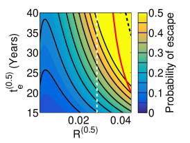
We now estimate the probability of shutdown of the monsoon in the model by projecting the system (13,14) onto a one-dimensional output ($\mathbf{w}^{T}=\mathbf{w}_{0}^{T}=(-3.50,-0.99)$) and expanding it near the fold to quadratic order (in $x$), and using the mode approximation estimate (23) for the escape probability. If time is measured in decades, the quadratic expansion of the monsoon model near its fold has the form $\dot{x}=p_{f}(A_{\mathrm{sys}}(t)-A_{\mathrm{sys}}^{b})+x_{f}x^{2}$ where $x$ is a dimensionless projection of the state. We add white noise of variance $2\Delta=\operatorname{diag}(0.02,6)$ to the monsoon model (13)–(14), such that

$$\mathrm{d}x=[p_{f}(A_{\mathrm{sys}}(t)-A_{\mathrm{sys}}^{b})+x_{f}x^{2}]\mathrm{d}t+\sqrt{2D}\mathrm{d}W_{t}\mbox{}$$ (24)

with the scaling factors $p_{f}=115.30$, $x_{f}=0.69$, and noise variance $D=3.04$. The albedo forcing functions $A_{\mathrm{sys}}(t)$ are chosen identical to equation (15)

$$A_{\mathrm{sys}}(t)=A_{\mathrm{sys}}^{\infty}+\frac{R^{(0.5)}+A_{\mathrm{sys}}^{\mathrm{th}}-A_{\mathrm{sys}}^{\infty}}{\cosh({\color[rgb]{0,0,0}S}(t_{\mathrm{end}}-2t))^{2}}\mbox{,}$$ (25)

where $A_{\mathrm{sys}}^{\infty}=0.47$ is the present-day value of the albedo and $[0,t_{\mathrm{end}}]$ is the time interval. For the same reasons as in the previous section, we choose a threshold lower than $A_{\mathrm{sys}}^{b}\approx 0.53$, specifically, $A_{\mathrm{sys}}^{\mathrm{th}}=0.5$, for measuring exceedance amplitudes and times. Hence, we consider the parameter plane $(R^{(0.5)},t^{(0.5)}_{e})$, where $R^{(0.5)}=R+A_{\mathrm{sys}}^{b}-0.5$ is the distance of the maximal albedo along the forcing from a chosen albedo threshold $A_{\mathrm{sys}}^{\mathrm{th}}=0.5$, and $t^{(0.5)}_{e}$ is the corresponding exceedance time above this threshold.

Figure 4(a) shows the mode approximation (23), using the solution $\bar{x}$ of $\dot{\bar{x}}=p_{f}(A_{\mathrm{sys}}(t)-A_{\mathrm{sys}}^{b})+x_{f}\bar{x}^{2}$ with (25), for the probability of escape $P_{\mathrm{esc}}^{\mathrm{1d}}$, on a grid of points in the $(R^{(0.5)},t^{(0.5)}_{e})$ - plane. Since the mode approximation (23) is valid only in the region to the left of the red line, Figure 4(a) leaves a part of the $(R^{(0.5)},t_{e}^{(0.5)})$-plane white. As before, the vertical white dashed line positioned indicates the location of the deterministic fold bifurcation and the black dashed curve provides the boundary for deterministic $(D=0)$ tipping.

(a)

(b)

(c)

Figure 4: Probability of escape: Contours in $(R^{(0.5)},t^{(0.5)}_{e})$ - plane and cross sections for two different values of $R^{(0.5)}$: $R^{(0.5)}=0.02$ (blue) and $R^{(0.5)}=0.03$ (red). (4(a)): Contour lines are spaced at $0.05$ intervals. White dashed line indicates the static fold bifurcation, black dashed curve shows the critical parameter values for deterministic tipping and the red solid curve indicates the boundary for validity of the mode approximation. (4(b)) Time profiles of planetary albedo scenarios of a short ($t^{(0.5)}_{e}=7.5$, and $9$ years for blue solid and red solid respectively) and longer ($t^{(0.5)}_{e}\approx 25$, and $30$ years for blue dashed and red dashed respectively) exceedance time $t^{(0.5)}_{e}$ for each fixed $R^{(0.5)}$ value. Horizontal black dotted line represents the chosen threshold value $A_{\mathrm{sys}}^{\mathrm{th}}=0.5$ used for the definition of $R^{(0.5)}$ and $t_{e}^{(0.5)}$. (4(c)) Probability of escape over a range of exceedance times $t_{e}^{(0.5)}$. Parameters: $\mathbf{w}=(-3.50,-0.99)^{T}$ such that $p_{f}=115.30$ and $x_{f}=0.69$ in (24), $D=3.04$.

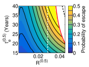
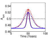
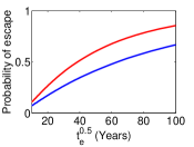
Consistent with the previous section and as expected we observe that for small $R^{(0.5)}$ and small $t^{(0.5)}_{e}$ the probability of escape is small. While, increasing $R^{(0.5)}$ (to and beyond the fold) and/or increasing the exceedance time $t^{(0.5)}_{e}$ over the arbitrary threshold the probability of escape increases.

Figure 4(c) shows the probability of escape for a range of times $t^{(0.5)}_{e}$ for which $A_{\mathrm{sys}}(t)$ is above the threshold $0.5$ for two fixed maxima $\max_{t}A_{\mathrm{sys}}(t)$. Figure 4(b) shows example scenarios of $A_{\mathrm{sys}}(t)$ with two different exceedance times for each fixed maximum.

6 Summary

We have investigated the scenario of forcing a system over a tipping threshold (a fold of equilibria) for a short time. We provide simple criteria determining whether the forced deterministic system escapes from the family of equilibria or not. The two primary parameters of the parameter forcing $q(t)$ are the maximum exceedance amplitude $\max_{t}q(t)$ beyond the fold bifurcation parameter value $q^{b}$, and the time $t_{e}$ for which the parameter forcing has exceeded the fold bifurcation value. The critical curve, which separates a region of tipping and the safe region in this two-parameter plane follows an inverse-square law: $t_{e}^{2}(\max_{t}q(t)-q^{b})=16/d^{b}$. The constant $d^{b}$ can be determined from equilibria at parameters $q$ near the critical value $q^{b}$ as the ratio of the square of the decay rate to $q-q^{b}$.

We used a simplified version of the Indian summer monsoon model developed by Zickfeld [11] to demonstrate which scenarios for changing planetary albedo in the model result in (or avoid) tipping, matching the general theoretical predictions (which are only accurate if one is sufficiently close to a fold) precisely: the trade-off between exceedance amplitude and time beyond the critical value of the albedo follows the inverse-square law with the predicted factor $d^{b}$.

We also quantify the effect of random disturbances, modeled by white additive noise, determining a probability of escape. For each chosen threshold $q_{0}$ near the fold we obtain level curves of equal probability in the parameter plane $(\max_{t}q(t)-q_{0},t_{e}^{0})$ of exceedance amplitude and exceedance time for $q_{0}$. These level curves follow the inverse-square law in part, deviating from it (expectedly) in the large-noise/slow-drift limit (for which we provide approximation formulas in the Supplementary Material) and at the origin of the $(\max_{t}q(t)-q_{0},t_{e}^{0})$.

This work did not involve any active collection of human data.

The research materials supporting this publication have been uploaded as part of the supplementary material.

P.R. derived the general mathematical results (with contributions from J.S.), processed and simplified the monsoon model, performed the numerical computations in sections 3 and 5, and led the writing of the paper. J.S. contributed to the mathematical results and performed the numerical computations in Section 4 and the fitting coefficients for approximations in the probabilistic results. O.K. carried out the comparison between approximations and simulations of the full model. All authors have contributed to the writing of the manuscript and gave final approval for publication.

We have no competing interests

P.R.’s research was supported by funding from the EPSRC Grant No. EP/M008495/1, P.R. has also received funding from the NERC grant No. NE/P007880/1. J.S. gratefully acknowledges the financial support of the EPSRC via Grants No. EP/N023544/1 and No. EP/N014391/1. J.S. has also received funding from the European Union’s Horizon 2020 research and innovation programme under Grant Agreement No. 643073.

We would like to thank Tim Lenton and Peter Cox for advice on the current consensus on the prospects of tipping in the Indian summer monsoon.

Appendix A Escape probability levels in transformed coordinates

The asymptotic behavior of the escape (tipping) probability for SDE (20) becomes visible after parameter transformation $(q_{1},q_{2})=(\sqrt{p_{2}},p_{0}-\sqrt{p_{2}})\in[0.1,4]\times[-2,2]$, shown in Figure 5.

Figure 5: Transformation of the $(p_{0},p_{2})$-parameter plane of Figure 3. for escape probability $P_{\mathrm{esc}}$ for $x\to+\infty$ in (20) with the transformation $q_{1}=\sqrt{p_{2}}$ and $q_{2}=p_{0}-\sqrt{p_{2}}$. Parameters for FPE (21): domain $[-8,8]$, time interval $[-T_{0},T_{0}]$, initial density $N(x_{0},1)$ where $T_{0}=\sqrt{(x_{0}^{2}+p_{0})/p_{2}}$ and $x_{0}=-4$. White dashed line indicates the static fold bifurcation, black dashed curve shows the critical parameter values for deterministic tipping and the red solid line indicates the boundary for validity of the single-mode approximation. Computed using chebfun [44].

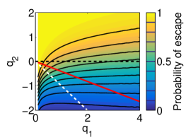
When one varies the noise variance $D$ in the original system (18), keeping the original forcing parameters $R_{0}$ and $R_{2}$ fixed, one moves along a straight line through the origin in Figure 5. An example is shown by a red line in Figure 5. The small-noise limit is at the large-$q_{1}$ end, and the large noise (or slow drift) limit is at the origin.

In the coordinates $(q_{1},q_{2})=(\sqrt{p_{2}},p_{0}-\sqrt{p_{2}})$ the slope of all $P_{\mathrm{esc}}$ level curves of equal probability will approach $0$ for large $q_{1}$ (or $\sqrt{p_{2}}$) such that the level curve for $P_{\mathrm{esc}}=0.5$ asymptotes to the horizontal $q_{2}=p_{0}-\sqrt{p_{2}}=0$ as at these parameter values the deterministic system has its tipping threshold (see (7) in Section 2), and the limit of large $q_{1}$ (or $p_{2}$) corresponds to the rapid drift (or small noise) limit. The $P_{\mathrm{esc}}$ level curves are graphs of functions $q_{2}(q_{1})$ in the coordinates of Figure 5. The slopes of these functions, $q_{2}^{\prime}(q_{1})$ go to zero for $q_{1}\to\infty$. This follows from the fact that in the small noise limit all probabilities with positive distance from $0$ or $1$ must get close to the deterministic tipping boundary. This deterministic tipping boundary corresponds to the ray $\{q_{2}=0,q_{1}>0\}$. Since the sets of fixed forcing parameters $R_{0}$ and $R_{2}$ and varying noise variances $2D$ correspond to rays, probabilities must converge to either $0$ or $1$ along each ray with $q_{2}\neq 0$. Hence, each probability contour level must cross all rays with non-zero slope.

Appendix B Projection and approximation error for the monsoon model

The projection of the SDE (16) to a one-dimensional system gives only accurate predictions for sufficiently small $\epsilon$, that is, for sufficiently small noise and slow parameter drift. We compare the predictions from the mode approximation of the projection onto the atmospheric temperature $T_{a}$ to the results of the two-dimensional monsoon model in the main paper, (3.1)–(3.2). To evaluate the tipping probability for the two-dimensional monsoon model we solve the Fokker-Planck equation

$$\partial_{t}u= D_{1}\partial_{Q_{a}}^{2}u+D_{2}\partial_{T_{a}}^{2}u-\partial_{Q_{a}}[f_{1}(Q_{a},T_{a},A_{\mathrm{sys}}(t))u]$$ (26)

$$-\partial_{T_{a}}[f_{2}(Q_{a},T_{a},A_{\mathrm{sys}}(t))u]$$

on the decade timescale with noise variances $D_{1}=0.01$ and $D_{2}=3$, and Dirichlet boundary conditions on the domain $(Q_{a},T_{a})\in[-0.04,0.07]\times[295,315]$ (so slightly larger than the physically realistic ranges). The forcings $A_{\mathrm{sys}}(t)$ are chosen as described in Section 3 and Section 5 of the main article, namely

$$A_{\mathrm{sys}}(t)=A_{\mathrm{sys}}^{\infty}+\frac{R^{(0.5)}+A_{\mathrm{sys}}^{\mathrm{th}}-A_{\mathrm{sys}}^{\infty}}{\cosh({\color[rgb]{0,0,0}S}(t_{\mathrm{end}}-2t))^{2}}\mbox{}$$ (27)

with $A_{\mathrm{sys}}^{\infty}=0.47$ (the approximate present day value), and $R$ and ${\color[rgb]{0,0,0}S}$ varying such that we exceed the threshold $A_{\mathrm{sys}}^{\mathrm{th}}=0.5$ for time $t_{e}^{(0.5)}\in[15,40]$ years and amplitude $R^{(0.5)}\in[0,0.045]$. For each simulation, we start from the eigenvector for the dominant (close to $1$) eigenvalue of the Fokker-Planck operator on the right-hand side of (26). The total simulation time period is chosen such that, after the transient time period, $A_{\mathrm{sys}}$ starts from close to its current day value, namely $0.471$, and returns back to this value again at the end of the total simulation period. The escape probability is then calculated as

$$P_{\mathrm{esc}}^{\mathrm{2d}}=1-\int_{Q_{a},T_{a}}u(Q_{a},T_{a},t_{\mathrm{end}})\mathrm{d}Q_{a}\mathrm{d}T_{a},$$ (28)

at the end of an overall integration period (neglecting the escape during the transient time period). The resulting escape probabilities are shown in Figure 6(a).

(a)

(b)

(c)

Figure 6: Comparison between the escape probability as computed from the full two-dimensional model to its projection and approximation (23) and slow drift approximation (S21) in the Supplementary Material. (a) Escape probability $P_{\mathrm{esc}}^{\mathrm{2d}}$, as computed using (26) and (28). (b) Difference between mode approximation depicted in Figure 4(a) of the main article calculated as $P_{\mathrm{esc}}^{\mathrm{1d}}-P_{\mathrm{esc}}^{\mathrm{2d}}$ and panel (a). (c) Difference between slow drift approximation of escape probability, $P_{\mathrm{esc}}^{\mathrm{slow}}$, and $P_{\mathrm{esc}}^{\mathrm{2d}}$. White dashed line indicates the fold bifurcation, black dashed curve the critical parameter values for deterministic tipping and the red solid curve indicates the boundary for validity of the mode approximation.

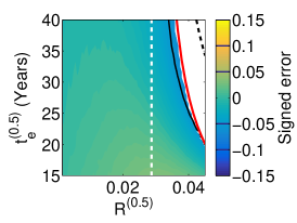
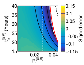
The one-dimensional projection of the monsoon model (6) is extracted from the output, temperature $T_{a}$, using a second-order approximation of the known equilibrium curve $(Q_{a},T_{a},A_{\mathrm{sys}})$ and the attraction rate toward stable equilibria nearby. In practice, these quantities may have to be estimated from observations or model outputs. Then we use a modification of (S16) from the Supplementary Material, replacing the parabolic forcing with the (rescaled) forcing of the planetary albedo (27):

$$\dot{x}=D^{-2/3}a_{0}^{2}\kappa(A_{\mathrm{sys}}(D^{-1/3}t)-A_{\mathrm{sys}}^{b})+x^{2}\mbox{.}$$ (29)

In Eq. (29) the forcing $A_{\mathrm{sys}}(t)$ is given by (27), $A_{\mathrm{sys}}^{b}\approx 0.5287$, $D=\mathbf{w}_{0}^{T}\operatorname{diag}(0.01,3)\mathbf{w}_{0}=3.04$ with $\mathbf{w}_{0}=(-3.50,-0.99)^{T}$, $\kappa\approx 6\cdot 10^{-3}$ and $a_{0}\approx 115.30$ ($a_{0}^{2}\kappa$ was estimated from decay rate and equilibrium curve of the 2d monsoon model.

The difference between the true escape probability (Figure 6(a)) and the mode approximation for the one-dimensional projected system (Figure 6(b)) is less than $0.05$ in absolute value everywhere in the region. The main source of error is that, due to the large noise variance, the system visits parts of the phase space where the quadratic approximation to the fold and the projection onto a single dimension are not accurate (the time scale separation between the two dimensions is only large close to the fold). For comparison, Figure 6(c) shows the slow-drift approximation, which is simply accumulating the escape rate for fixed parameter $A_{\mathrm{sys}}$ over the interval (see Supplementary Material for precise formulas). We observe that the mode approximation has a systematically smaller error especially close to the fixed-$A_{\mathrm{sys}}$ bifurcation point (white dashed line).

Appendix C Monsoon parameters

Section 3 discussed a simplification to the Indian summer monsoon model used by Zickfeld [11], retaining the key dynamics behind the mechanisms of the monsoon. Table 1 lists all the parameters and their values used in the simplified monsoon model.

Table 1: Table of parameters used in Indian summer monsoon model

Parameter	Value	Unit	Description
$T_{oc}$	$300$	$K$	temperature over Indian Ocean
$T_{0}$	$273.2$	$K$	freezing point
$Q_{oc}$	$0.0190$	$1$	humidity over Indian Ocean
$Q_{\mathrm{sat}}$	$0.0401$	$1$	saturated humidity
$\mathcal{L}$	$2.5\times 10^{6}$	$m^{2}s^{-2}$	latent heat
$C_{E}$	$3.4375\times 10^{-4}$	$mm\,s^{-1}K^{-1}$	evaporation factor
$C_{P}$	$0.0027$	$mm\,s^{-1}$	precipitation factor
$C_{mo}$	$6.9021\times 10^{-4}$	$mm\,s^{-1}K^{-1}$	moisture advection factor ocean
$C_{ml}$	$1.6213\times 10^{-4}$	$mm\,s^{-1}K^{-1}$	moisture advection factor land
$C_{L1}$	$1.6642$	$Kg\,s^{-3}K^{-1}$	outgoing long-wave radiation factor
$C_{L2}$	$-263.3753$	$Kg\,s^{-3}$	outgoing long-wave radiation constant
$F_{\downarrow}^{SL,TA}$	$443.6250$	$Kg\,s^{-3}$	incoming short wave radiation factor
$C_{H}$	$0.7136$	$Kg\,s^{-3}\,K^{-2}$	heat advection factor
$\theta_{oc}$	$300.2356$	$K$	potential temperature over Indian Ocean
$\Gamma_{0}$	$0.0053$	$K\,m^{-1}$	atmospheric lapse rate constant
$\Gamma_{1}$	$5.5\times 10^{-5}$	$m^{-1}$	atmospheric lapse rate linear factor
$\Gamma_{2}$	$1000$	$1$	atm. lapse rate quadratic factor for $Q_{a}$
$\Gamma_{a}$	$0.0098$	$K\,m^{-1}$	rate of decrease for pot. temp. over land
$z_{h}$	$5.1564\times 10^{3}$	$m$	high altitude fixed in model
$I_{q}$	$2.0636\times 10^{3}$	$mm$	humidity scaling factor
$I_{T}$	$1.1958\times 10^{9}$	$Kg\,s^{-2}\,K^{-1}$	temperature scaling factor
$\beta$	$3.1710\times 10^{-9}$	decades$\,s^{-1}$	time scaling factor

References

- Lenton et al. [2008] Timothy M Lenton, Hermann Held, Elmar Kriegler, Jim W Hall, Wolfgang Lucht, Stefan Rahmstorf, and Hans Joachim Schellnhuber. Tipping elements in the Earth’s climate system. Proceedings of the National Academy of Sciences, 105(6):1786–1793, 2008.
- Held and Kleinen [2004] Hermann Held and Thomas Kleinen. Detection of climate system bifurcations by degenerate fingerprinting. Geophysical Research Letters, 31(23), 2004.
- Holland et al. [2006] Marika M Holland, Cecilia M Bitz, and Bruno Tremblay. Future abrupt reductions in the summer Arctic sea ice. Geophysical Research Letters, 33(23), 2006.
- Boulton et al. [2014] Chris A Boulton, Lesley C Allison, and Timothy M Lenton. Early warning signals of Atlantic Meridional Overturning Circulation collapse in a fully coupled climate model. Nature Communications, 5, 2014.
- Laurance et al. [2011] William F Laurance, Bernard Dell, Stephen M Turton, Michael J Lawes, Lindsay B Hutley, Hamish McCallum, Patricia Dale, Michael Bird, Giles Hardy, Gavin Prideaux, et al. The 10 Australian ecosystems most vulnerable to tipping points. Biological Conservation, 144(5):1472–1480, 2011.
- Clark et al. [2013] Graeme F Clark, Jonathan S Stark, Emma L Johnston, John W Runcie, Paul M Goldsworthy, Ben Raymond, and Martin J Riddle. Light-driven tipping points in polar ecosystems. Global Change Biology, 19(12):3749–3761, 2013.
- Siteur et al. [2014] Koen Siteur, Eric Siero, Maarten B Eppinga, Jens DM Rademacher, Arjen Doelman, and Max Rietkerk. Beyond turing: The response of patterned ecosystems to environmental change. Ecological Complexity, 20:81–96, 2014.
- Gandhi et al. [2015] Punit Gandhi, Edgar Knobloch, and Cédric Beaume. Localized states in periodically forced systems. Physical review letters, 114(3):034102, 2015.
- Yan et al. [2010] Wanfeng Yan, Ryan Woodard, and Didier Sornette. Diagnosis and prediction of tipping points in financial markets: Crashes and rebounds. Physics Procedia, 3(5):1641–1657, 2010.
- Ashwin et al. [2017] Peter Ashwin, Clare Perryman, and Sebastian Wieczorek. Parameter shifts for nonautonomous systems in low dimension: Bifurcation-and rate-induced tipping. Nonlinearity, 30(6):2185, 2017.
- Zickfeld [2004] Kirsten Zickfeld. Modeling large-scale singular climate events for integrated assessment. PhD thesis, Universitätsbibliothek, 2004.
- Levermann et al. [2009] Anders Levermann, Jacob Schewe, Vladimir Petoukhov, and Hermann Held. Basic mechanism for abrupt monsoon transitions. Proceedings of the National Academy of Sciences, 106(49):20572–20577, 2009.
- Zickfeld et al. [2005] Kirsten Zickfeld, B Knopf, V Petoukhov, and HJ Schellnhuber. Is the Indian summer monsoon stable against global change? Geophysical Research Letters, 32(15), 2005.
- Berglund and Gentz [2006] Nils Berglund and Barbara Gentz. Noise-induced phenomena in slow-fast dynamical systems: a sample-paths approach. Springer Science & Business Media, 2006.
- Majumdar et al. [2013] Apala Majumdar, John Ockendon, Peter Howell, and Elena Surovyatkina. Transitions through critical temperatures in nematic liquid crystals. Physical Review E, 88(2):022501, 2013.
- Lenton [2011] Timothy M Lenton. Early warning of climate tipping points. Nature Climate Change, 1(4):201–209, 2011.
- Hawkins et al. [2011] Ed Hawkins, Robin S Smith, Lesley C Allison, Jonathan M Gregory, Tim J Woollings, Holger Pohlmann, and B De Cuevas. Bistability of the atlantic overturning circulation in a global climate model and links to ocean freshwater transport. Geophysical Research Letters, 38(10), 2011.
- Zhu et al. [2015] Jiang Zhu, Zhengyu Liu, Jiaxu Zhang, and Wei Liu. AMOC response to global warming: dependence on the background climate and response timescale. Climate Dynamics, 44(11-12):3449–3468, 2015.
- Li et al. [2016a] Xichen Li, Shang-Ping Xie, Sarah T Gille, and Changhyun Yoo. Atlantic-induced pan-tropical climate change over the past three decades. Nature Climate Change, 6(3):275, 2016a.
- Ditlevsen and Johnsen [2010] Peter D Ditlevsen and Sigfus J Johnsen. Tipping points: early warning and wishful thinking. Geophysical Research Letters, 37(19), 2010.
- Aalen et al. [2008] Odd Aalen, Ornulf Borgan, and Hakon Gjessing. Survival and event history analysis: a process point of view. Springer Science & Business Media, 2008.
- Scheffer et al. [2009] Marten Scheffer, Jordi Bascompte, William A Brock, Victor Brovkin, Stephen R Carpenter, Vasilis Dakos, Hermann Held, Egbert H Van Nes, Max Rietkerk, and George Sugihara. Early-warning signals for critical transitions. Nature, 461(7260):53–59, 2009.
- Dakos et al. [2008] Vasilis Dakos, Marten Scheffer, Egbert H van Nes, Victor Brovkin, Vladimir Petoukhov, and Hermann Held. Slowing down as an early warning signal for abrupt climate change. Proceedings of the National Academy of Sciences, 105(38):14308–14312, 2008.
- Scheffer et al. [2012] Marten Scheffer, Stephen R Carpenter, Timothy M Lenton, Jordi Bascompte, William Brock, Vasilis Dakos, Johan Van De Koppel, Ingrid A Van De Leemput, Simon A Levin, Egbert H Van Nes, et al. Anticipating critical transitions. science, 338(6105):344–348, 2012.
- Ritchie and Sieber [2016] Paul Ritchie and Jan Sieber. Early-warning indicators for rate-induced tipping. Chaos, 26(9):093116, 2016. http://dx.doi.org/10.1063/1.4963012.
- Kuznetsov [2004] Y. A Kuznetsov. Elements of Applied Bifurcation Theory, volume 112 of Applied Mathematical Sciences. Springer-Verlag, New York, third edition, 2004. ISBN 0-387-21906-4.
- Kuehn [2015] Christian Kuehn. Multiple Time Scale Dynamics. Springer, 2015.
- Neishtadt [1987] AI Neishtadt. Persistence of stability loss for dynamical bifurcations. 1. Differential Equations, 23(12):1385–1391, 1987.
- Neishtadt [1988] AI Neishtadt. Persistence of stability loss for dynamical bifurcations. 2. Differential Equations, 24(2):171–176, 1988.
- Baesens [1991] Claude Baesens. Slow sweep through a period-doubling cascade: Delayed bifurcations and renormalisation. Physica D: Nonlinear Phenomena, 53(2-4):319–375, 1991.
- Baer et al. [1989] Steven M Baer, Thomas Erneux, and John Rinzel. The slow passage through a hopf bifurcation: delay, memory effects, and resonance. SIAM Journal on Applied mathematics, 49(1):55–71, 1989.
- Li et al. [2016b] J Li, Felix X-F Ye, Hong Qian, and Sui Huang. Time dependent saddle node bifurcation: Breaking time and the point of no return in a non-autonomous model of critical transitions. arXiv preprint arXiv:1611.09542, 2016b.
- Ritchie and Sieber [2017] Paul Ritchie and Jan Sieber. Probability of noise- and rate-induced tipping. Phys. Rev. E, 95:052209, 2017.
- Lenton et al. [2012] TM Lenton, VN Livina, V Dakos, EH Van Nes, and M Scheffer. Early warning of climate tipping points from critical slowing down: comparing methods to improve robustness. Philosophical Transactions of the Royal Society of London A: Mathematical, Physical and Engineering Sciences, 370(1962):1185–1204, 2012.
- O’Riordan and Lenton [2013] Timothy O’Riordan and Timothy Lenton. Addressing tipping points for a precarious future. Oxford University Press, 2013.
- Bhat [2006] Ganesh S Bhat. The indian drought of 2002—a sub-seasonal phenomenon? Quarterly Journal of the Royal Meteorological Society, 132(621):2583–2602, 2006.
- Liepert and Giannini [2015] Beate G Liepert and Alessandra Giannini. Global warming, the atmospheric brown cloud, and the changing indian summer monsoon. Bulletin of the Atomic Scientists, 71(4):23–30, 2015.
- Ramanathan et al. [2005] Veerabhadran Ramanathan, C Chung, D Kim, T Bettge, L Buja, JT Kiehl, WM Washington, Q Fu, DR Sikka, and M Wild. Atmospheric brown clouds: Impacts on south asian climate and hydrological cycle. Proceedings of the National Academy of Sciences of the United States of America, 102(15):5326–5333, 2005.
- Auffhammer et al. [2006] Maximilian Auffhammer, V Ramanathan, and Jeffrey R Vincent. Integrated model shows that atmospheric brown clouds and greenhouse gases have reduced rice harvests in india. Proceedings of the National Academy of Sciences, 103(52):19668–19672, 2006.
- Meehl et al. [2008] Gerald A Meehl, Julie M Arblaster, and William D Collins. Effects of black carbon aerosols on the indian monsoon. Journal of Climate, 21(12):2869–2882, 2008.
- Knopf et al. [2006] B Knopf, M Flechsig, and K Zickfeld. Multi-parameter uncertainty analysis of a bifurcation point. Nonlinear Processes in Geophysics, 13(5):531–540, 2006.
- Hatzianastassiou et al. [2004] N Hatzianastassiou, A Fotiadi, Ch Matsoukas, K Pavlakis, E Drakakis, D Hatzidimitriou, and I Vardavas. Long-term global distribution of earth’s shortwave radiation budget at the top of atmosphere. Atmospheric Chemistry and Physics, 4(5):1217–1235, 2004.
- Risken and Frank [2012] Hannes Risken and Till Frank. The Fokker-Planck Equation: Methods of Solution and Applications. Springer Science & Business Media, 2012.
- Driscoll et al. [2014] Tobin A Driscoll, Nicholas Hale, and Lloyd N Trefethen. Chebfun guide. Pafnuty Publications, Oxford, http://www.chebfun.org/, 2014.
- Hänggi et al. [1990] Peter Hänggi, Peter Talkner, and Michal Borkovec. Reaction-rate theory: fifty years after Kramers. Reviews of modern physics, 62(2):251, 1990.