Initial System-Environment Correlations via the Transfer Tensor Method
Abstract
Open quantum systems exhibiting initial system-environment correlations are notoriously difficult to simulate. We point out that given a sufficiently long sample of the exact short-time evolution of the open system dynamics, one may employ transfer tensors for the further propagation of the reduced open system state. This approach is numerically advantageous and allows for the simulation of quantum correlation functions in hardly accessible regimes. We benchmark this approach against analytically exact solutions and exemplify it with the calculation of emission spectra of multichromophoric systems as well as for the reverse temperature estimation from simulated spectroscopic data. Finally, we employ our approach for the detection of spectral signatures of electromagnetically-induced transparency in open three-level systems.
I Introduction
The simulation of reduced open quantum systems is usually facilitated by the assumption of at least an initial product state between the system and its environment at some initial point in time Breuer and Petruccione (2002); Weiss (2012). However, numerous questions crucially require to account for initial correlations between the open system of interest and its environment. Apart from witnessing or certifying their existence Laine et al. (2010); Rodríguez-Rosario et al. (2012); Chaudhry and Gong (2013); Ringbauer et al. (2015); Vinjanampathy and Modi (2015); Chen and Goan (2016), they find very concrete applications such as the correct simulation of emission spectra of molecular systems Ma and Cao (2015); Ma et al. (2015); Moix et al. (2015) or their thermodynamic effect for the extractable work of thermal machines Alicki and Fannes (2013); Perarnau-Llobet et al. (2015). Although it has recently been pointed out that correlations may play a relevant role already in the weak system-environment coupling regime Chaudhry and Gong (2013), it is in situations of strong coupling to a non-Markovian environment where initial correlation effects are expected to be most significant. In this regime, it becomes necessary to resort to specialized treatments, see e.g. Refs. Grabert et al. (1988); Pechukas (1994); Esposito and Gaspard (2003); Iles-Smith et al. (2014); Chen and Goan (2016); Halimeh and de Vega (2017); Strasberg et al. (2016), at the expense of enhanced computational effort.
Here, methods such as the stochastic Liouville-von Neumann equations (SLE) Stockburger and Grabert (2002); Song and Shi (2015) or the hierarchy of equations of motion technique (HEOM) Tanimura and Kubo (1989); Tanimura (2014) stand out. SLE is based on the sampling of environmental trajectories in terms of stochastic realizations. The number of required trajectories generally scales with the length of the simulation time rather than with the strength of the coupling to the environment, its spectral density or its temperature, and it is therefore well suited for short but accurate simulations. In contrast, HEOM scales with the number of exponential functions required to approximate the environmental correlation functions and with the coupling strength. For this reason, it is best suited for high-temperature baths and Lorentzian spectral densities.
Strategies to circumvent the unfavorable scaling have been put forward Stockburger (2016). In this context, the transfer tensor method (TTM) Cerrillo and Cao (2014) provides a powerful tool to extend simulations to very long times Rosenbach et al. (2016). It can be interpreted as a discrete representation of the Nakajima-Zwanzig equation and has additionally found applications to mixed quantum-classical methods Kananenka et al. (2016). While originally transfer tensors are obtained from simulations of separable initial states, here we demonstrate how they can be correctly applied to account for a large class of initial system-environment correlations. This enables us to efficiently compute two-time correlation functions in the steady state such as absorption and emission spectra, as illustrated in Fig. 1. The class of initial states that are accessible with the method can be regarded as preparative transformations of the global thermal system-environment state. We restrict ourselves to preparative transformations that affect only the system but are otherwise general, including e.g. a measurement performed on the open system or system-local unitary transformations.
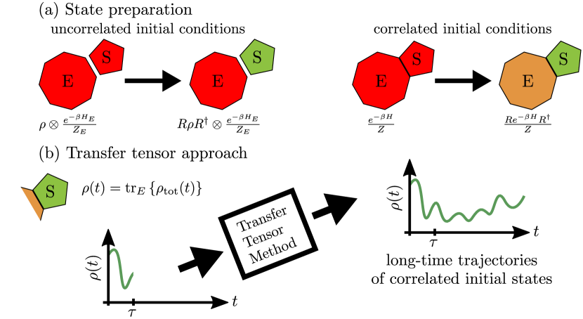
In the following, we first illustrate in Sec. II the breakdown of the quantum regression theorem by exploring how within a HEOM simulation the effect of initial correlations becomes increasingly relevant in the strong-coupling and slow-environment regime. In Sec. III, we demonstrate that correlated initial states can be treated with TTM, where a successful benchmark of the joint TTM-HEOM approach is also presented. In Sec. IV, we apply the proposed TTM approach for correlated initial states to the calculation of emission spectra of multichromophoric systems in previously hardly accessible regimes. Additionally, a detailed balance relation between absorption and emission spectra is employed for successful temperature estimation from simulated spectra. Finally, we use the TTM-SLE approach for the detection of spectral signatures of electromagnetically induced transparency in an open three-level system in Sec. V.
II Breakdown of the quantum regression theorem
We illustrate that the effect of initial correlations becomes especially relevant for systems located beyond the weak-coupling regime or systems that feature large correlation times of the environment. This is formally equivalent to the breakdown of the quantum regression theorem. We consider systems that are described in terms of a total Hamiltonian , comprised of a system (), interaction () and environmental () part, . The correlated initial states of interest are obtained from the thermal system-environment state, characterized by an inverse temperature , and subsequently transformed by a preparative procedure ,
| (1) |
where only affects the system. We will use a notation where denotes the total density matrix, and where the partition functions corresponding to the total system thermal state and the thermal environmental state are given by . The reduced state describing the open system of interest is then obtained from the total system state by tracing out the environmental degrees of freedom, . Regarding the preparative procedures, they may be of the form of a projective measurement performed on the open system, so that with being the projector associated to the respective measurement outcome. Alternatively, might also denote a unitary transformation that acts on the open system subspace only. Any admissible transformation for a density matrix is suitable as long as it is applied locally on the system (Kraus map) Kraus (1983). From now on, we will set the initial time to zero for simplicity, .
It is often assumed that within the weak system-environment coupling regime, the effect of the preparative procedure Eq.(1) onto the environment can be safely neglected and the correlated initial states can consequently be well approximated by means of the usual initial product state assumption
| (2) |
Fig. 1 (a) provides a sketch of the considered setup. In order to verify that the error introduced with Eq.(2) generally grows with the coupling between the open system and its environment as well as with characteristic environmental correlation times, we present numerical results obtained for a spin-boson model governed by the Hamiltonian
| (3) |
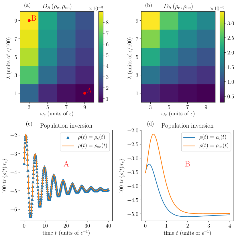
Here, denotes the energetic splitting of the two bare levels, denotes the tunneling amplitude, and denotes the collective position of the bosonic environment described by , with creation and annihilation operators and for environmental modes with associated energies . The coupling to the individual environmental modes is parametrized by . The usual Pauli matrices are denoted by , the normalized eigenvectors of are defined by and . For the results presented in Figure 2, characteristic bath correlation functions of the form with coupling strength and reservoir cutoff have been employed. These correlation functions are suitable for the HEOM formalism and approximate the effect of a Drude-Lorentz bath, described by a spectral density , in the high-temperature regime Ishizaki and Fleming (2009). Thereby, the reorganization energy quantifies the overall coupling strength between the two-level system and its environment and is inversely proportional to the characteristic correlation time of the latter.
The time evolution of the reduced open system state corresponding to the correlated initial condition Eq.(1), , and the evolution of the reduced state corresponding to the uncorrelated initial condition Eq.(2), , are compared in Fig. 2. Their difference is quantified by means of the cumulative trace distance defined as , with denoting the usual trace distance. From this definition one can already infer that the cumulative trace distance would diverge if differences between and prevail at steady state. The considered correlated initial states are given by means of a unitary rotation of the total system thermal state according to Eq. (1) with (panel (a), (c) and (d)) or by means of an ideal measurement performed on the open system yielding an outcome associated to the open system state , such that the projector as described above is given by (panel (b)). The upper plots (a) and (b) in Fig. 2 point out that the error introduced with Eq. (2) systematically increases when increasing the system-environmental coupling strength or the characteristic correlation time of the environment . Panels (c) and (d) compare the effect of these initial correlations in terms of the time evolution of the population inversion for parameter sets A and B marked in panel (a).
III Initial correlations via the transfer tensor method
In discrete time, the evolution of any reduced open system state can be expressed in terms of the transfer tensor formalism Cerrillo and Cao (2014) in the following generalized form
| (4) |
with transfer tensors corresponding to the evolution of an initial product state and a correction that accounts for the effect of initial correlations between the system and its environment. Here, the transfer tensors are defined recursively by with and dynamical maps that determine the evolution of an open system given an initial separable state of the form , such that . We emphasize that the tensors carry key information about the underlying dynamics of the open system state as they manifest a discrete representation of the Nakajima-Zwanzig memory kernel within the reduced open system subspace.
Here, we propose the use of transfer tensors for correlated initial states in the following manner:
-
•
First, the transfer tensors corresponding to an initial product state featuring a thermal bath are learned from a suitable simulation method of choice.
-
•
In a second step, the reduced density matrix corresponding to the correlated initial state of interest is propagated up to some time covering at least the length of the memory kernel, such that . This step can be conducted by means of any appropriate numerically exact simulation method, for instance by integrating the SLE Stockburger and Grabert (2002) or HEOM Tanimura (2014).
-
•
Third, the correction term that quantifies the effect of initial correlations onto the dynamics can be determined. A sufficient decay of within the simulation time verifies the suitability of the final step: a subsequent efficient propagation by means of the transfer tensors only.
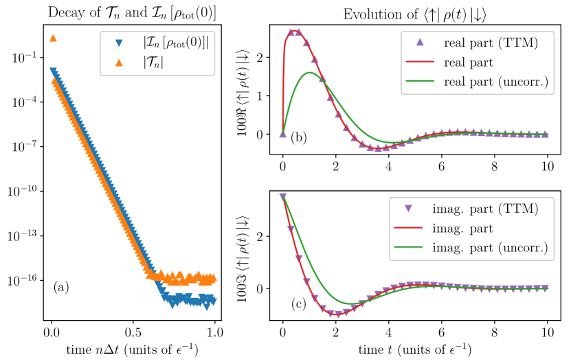
This approach is illustrated in Fig. 3 and benchmarked in combination with HEOM against exact results. For this, an exactly solvable variant of the spin boson model Eq.(3), given by
| (5) |
with a characteristic environmental correlation function is considered. The evolution of a correlated initial state with is shown in panels (b) and (c), by means of the real and imaginary part of the reduced density matrix element . The result obtained when considering an uncorrelated initial state is additionally shown for comparison. The large discrepancies between initially correlated and uncorrelated simulations are mostly due to the strong system-environment coupling and further reveal the necessity to account for initial correlations. Remarkable agreement is shown between the exact and the TTM-HEOM results. Panel (a) further verifies the suitability of the approach by showing the decay of the transfer tensors and the correction term within the range to . In view of the strong suppression over several orders of magnitude, the reduced open system state can be safely further propagated in time by means of transfer tensors as described above.
We emphasize that the verification of the suitability of the presented transfer tensor method for correlated initial states can be ensured by monitoring the required decays of the inhomogeneous contribution and the transfer tensors – even for models that do not allow for an exact solution. Sufficient decays have been verified for all of the presented results.
IV Application: Emission spectra of multichromophoric systems
As we will see, the calculation of emission spectra of multichromophoric systems provides an application that most importantly requires to account for correlated initial states. Here, we refer to systems that have been extensively discussed in Refs. Ma and Cao (2015); Ma et al. (2015); Moix et al. (2015). The molecular systems of interest are modeled by means of internal excited states , that span a single-exciton manifold and that are coupled diagonally to the collective positions of their individual bosonic environments. Additionally, these systems feature an internal ground state, denoted by , that is uncoupled from the excited states and their thermal baths in the Hamiltonian description. However, transitions between the excited manifold and the internal ground state can be formally incorporated by interactions with a further generic environment of the form , with system dipole operator
| (6) |
and some arbitrary environment operator . Omitting this further environment from the discussion, the corresponding Hamiltonian reads as
| (7) |
with a a total number of independent bosonic baths, , and their collective positions . The open system Hamiltonian representing the single-exciton manifold reads as
| (8) |
and allows for interactions among the excited states. Emission and absorption spectra are generically linked to transitions between the internal excited states and the ground state. They are obtained by computing Fourier transforms of the respective dipole-dipole correlation functions Ma and Cao (2015), and with
| (9) | ||||
| (10) |
Here, denotes the time-evolved dipole operator. The considered initial state for absorption processes is a product state composed of the internal ground state and thermal bath states. It can be obtained from the global thermal state by means of a projection onto the ground state, . Here, denotes the normalized projector onto the ground state, with . For emission processes on the other hand, a correlated initial thermal state that is equilibrated within the excited subspace needs to be considered. It is defined as the projection of the global thermal state onto the excited subspace , with and . This state may be prepared by optical pumping Kastler (1967) or similar procedures. We note that such transitions between the excited and the ground manifold are beyond Eq. (7) but would e.g. correspond to the linear response effect of the system on additional environmental modes.
The absorption and emission spectra fulfill a Kubo-Martin-Schwinger like relation
| (11) |
with , and which translates into the frequency domain as
| (12) |
This can be derived from the form of the dipole operators, and , together with the fact that the total Hamiltonian does not couple the ground state with the excited manifold, , and it fulfills and . As a consequence, the absorption and emission dipole-dipole correlation functions can be rewritten as and with reduced absorption and emission operators
| (13) | ||||
| and | ||||
| (14) | ||||
These matrices fulfill the Kubo-Martin-Schwinger like relationship also elementwise. Most importantly, relationship Eq. (12) has proven useful for the simplification of the derivation of multicromophoric spectra Chenu and Cao (2017) and can in our case be employed for temperature estimation from spectroscopic data and for the validation of results obtained from numerical simulations as shown in Figs. 5 and 6.
In a series of previous papers Ma and Cao (2015); Ma et al. (2015); Moix et al. (2015), the simulation of the reduced absorption and emission operators by means of different perturbative methods, such as the full cumulant expansion and hybrid cumulant expansion, as well as numerically exact methods, such as the stochastic path integral formalism or HEOM and its stochastic extension Moix and Cao (2013), has been discussed in detail. It turns out that, for general parameters, the stochastic path integral (sPI) approach Moix et al. (2015) manifests itself as a very powerful technique: it is not restricted to high temperatures or certain forms of the environmental spectral densities and it is suitable for the strong system-environment coupling regime. We point out that it constitutes a simpler method than SLE for density matrices Stockburger and Grabert (2002) due to the one-sided form of the evolution of the reduced absorption and emission operators, see Eq. (13) and Eq. (14). However, obtaining converged results for long-lasting system dynamics remains a cumbersome task. For the case of absorption spectra, this difficulty can be overcome by means of the usual TTM approach Rosenbach et al. (2016). Here, we extend this result and address the emission operator with the presented TTM approach for correlated initial states. We instantiate the proposed method with a molecular system that exhibits excited states and is described by the system Hamiltonian
| (15) |
expressed in the basis . Consequently, we consider two independent but identical baths that are coupled to the excited states. Each of them shall be characterized by an ohmic spectral density with an exponential cutoff for .
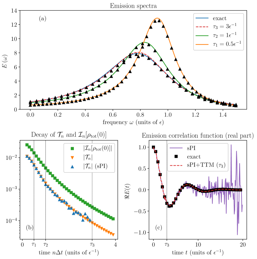
For a diagonal system Hamiltonian, , the emission problem can be solved exactly and may be used for the systematic benchmark of our TTM-sPI approach for correlated initial conditions that is presented in Fig. 4. Panel (a) shows the exact emission spectrum (blue line) and the rapid convergence of TTM towards the exact result with increasing sample times (red, green and yellow lines), where it is shown that a sample time of is sufficient to recover the exact result. The increase in the sample time gradually broadens the spectrum and its maxima is shifted to lower frequencies. This trend is representative of an effective increase of the system-environmental coupling as a larger portion of the memory kernel is represented by the transfer tensors. This view is supported by panel (b) which shows the decay of the transfer tensors (yellow triangles). It also shows the rapid decay of the effect of initial correlations (green squares) of approximately two orders of magnitude by the time . Panel (c) illustrates the difficulty to access long time propagation of the emission correlation function by means of a sPI simulation (purple line), whereas transfer tensors learned from a short-time sPI simulation suffice to accurately propagate to long times (red dashed line).
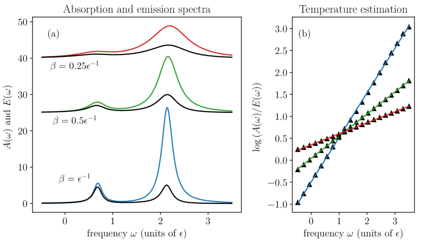
The symmetry relation between absorption and emission spectra Eq.(12) allows for thermometry based on spectroscopic data and also for the validation of the results stemming from numerical simulations such as our joint TTM-sPI approach. By means of this relation, the environmental temperature as well as the ratio of the partition functions can be immediately recovered from the corresponding spectra as illustrated in Fig. 5. Therein, we consider the Hamiltonian
| (16) |
In panel (a) emission and absorption spectra are shown for three different temperatures (low), (intermediate) and (high). All of the presented emission (black lines) and absorption (colored lines) spectra show peaks at frequencies that can be roughly identified with the two eigenvalues of the system Hamiltonian given by and , which can be best recognized in the low temperature example. The intermediate and high temperature cases exhibit an enhanced occupation of energetically higher environmental states, which supports transitions between ground and the excited states and vice versa on a wider energetic range. This results in a general broadening of the spectra. Additionally, one finds that for the low temperature example, the two emission peaks show roughly the same height, whereas for increasing temperatures one observes an increasing imbalance in favor of the peak associated to the higher energy. Panel (b) shows that successful estimation of the temperature from the simulated data is possible when initial correlations are taken into account.
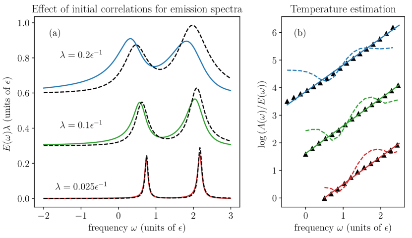
The presented TTM approach for correlated initial conditions allows for detailed studies of the importance of initial correlations for emission spectra by means of the possibility of accounting fully or partially, or even neglecting, the corresponding effects. In practice, this can be achieved by truncating the length of the initial sample of the exact (initially correlated) evolution of that is used. This is shown in Fig. 6 (a), where approximate emission spectra are presented which are obtained from a simulation that neglects the effect of initial correlations by means of a propagation of a sample of that only has length one. For weak system-environment couplings, one expects the effect of initial correlations to be negligible and this is indeed the case for , for which the approximate emission spectrum (black dashed line) provides a qualitatively good estimate for the exact emission spectrum (red line). However, with increasing system-environmental coupling strength, the effect of initial correlations becomes more relevant for the reduced emission operator and the approximate spectra fail to estimate the exact result. More importantly, we stress that even for the weak-coupling case () the temperature cannot be faithfully recovered from the approximate spectrum as shown in panel (b). Temperature estimation from the simulated spectra crucially requires to account for initial correlations of the reduced emission operator .
V Application: Spectral signatures of electromagnetically induced transparency
We finally employ the joint TTM-sPI approach for the investigation of spectral signatures of electromagnetically induced transparency (EIT). EIT is the phenomenon of vanishing absorption or emission due to the coupling of the dissipative manifold to a discrete state, and has found extensive application in the enhancement of laser cooling schemes for trapped ions Morigi et al. (2000). It appears in a so-called lambda configuration, where an excited state is coupled in Raman resonance with two ground states and forming the following system Hamiltonian
| (17) |
For the case , the basis of the dark state and bright state allows us to represent Hamiltonian Eq.(18) in the form Eq.(15). We will investigate the specific case
| (18) |
where the matrix is represented in the basis.
This three-level system is coupled to the collective position of a bosonic environment in dipolar form, such that the total Hamiltonian of the considered setup reads as
| (19) |
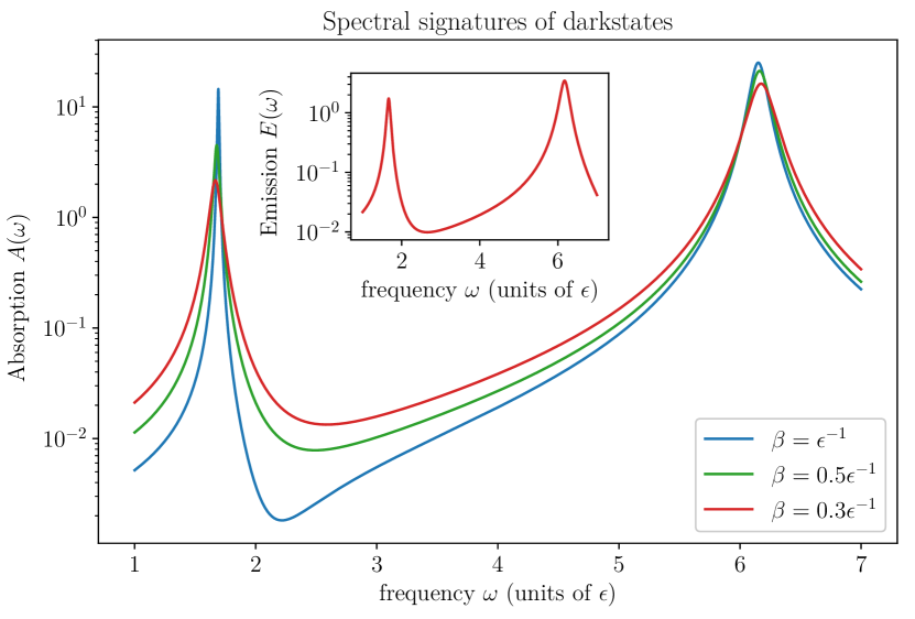
The coupling to the individual environmental modes shall be parametrized by an Ohmic spectral density with an exponential cutoff . We focus on the corresponding emission and absorption spectra for the dipole operator definition that show signatures of electromagnetically induced transparency. Absorption spectra are shown in Fig. 7 when considering three different temperatures of the environment. The characteristic dip indicating the presence of a dark state at becomes most obvious for low temperatures of the environment. However, even for the highest considered temperature the characteristic suppression can be observed within the corresponding emission spectrum.
We note that the presented TTM-sPI approach is especially well suited for studies of the parameter-regime considered in Fig 7. This is because of the long-lasting system dynamics due to the weak system-environmental coupling and the low temperatures. The considered parameter regime could otherwise not be treated with the usual stochastic path integral method.
VI Summary
Successful TTM-sPI and TTM-HEOM approaches for the simulation of open quantum systems subject to correlated initial conditions have been presented in this paper. The TTM approach for correlated initial conditions is especially useful for settings that feature low-temperatures or intermediate system-environment couplings, such that the reduced open system state of interest evolves on a time scale that is large compared to the characteristic correlation time of the environment.
We note that originally, TTM has been introduced for open systems that are subject to uncorrelated initial conditions. For the class of correlated initial conditions considered in this paper, it is still possible to apply TTM without any significant overhead. Recently, it has been pointed out that the formalism can in principle be extended in order to include correlated initial states by expressing them as a linear combination of a maximum of system-environment product terms Pollock and Modi (2017), where denotes the open system Hilbert space dimension. For each of the terms, the original TTM can be applied individually, leading to a set of transfer tensors that propagate the individual terms. Nevertheless, a practical implementation of the concept remains pending and the required overhead involving the derivation of transfer tensors could render it a challenging task.
Considering absorption and emission spectra of multichromophoric systems, we have shown that the symmetry relation Eq. (12) allows for successful temperature estimation from simulated spectroscopic data. In this context it turned out to be crucial to account for initial correlations of the reduced emission operator – even in the weak system-environment coupling regime.
Finally, the joint TTM-sPI approach enables the exploration of spectral signatures of electromagnetically induced transparency within obtained absorption and emission spectra in hardly accessible regimes.
Acknowledgements.
The authors would like to acknowledge financial support from the DFG projects BR 1528/9-1, SCHA 1646/3-1, SFB 910, GRK 1558. M.B. acknowledges financial support from the Studienstiftung des Deutschen Volkes.References
- Breuer and Petruccione (2002) H.-P. Breuer and F. Petruccione, The Theory of Open Quantum Systems (Oxford University Press, 2002).
- Weiss (2012) U. Weiss, Quantum Dissipative Systems, Vol. 13 (World Scientific, 2012).
- Laine et al. (2010) E.-M. Laine, J.Piilo, and H.-P. Breuer, EPL (Europhysics Letters) 92, 60010 (2010).
- Rodríguez-Rosario et al. (2012) C. A. Rodríguez-Rosario, K. Modi, L. Mazzola, and A. Aspuru-Guzik, EPL (Europhysics Letters) 99, 20010 (2012).
- Chaudhry and Gong (2013) A. Z. Chaudhry and J. Gong, Phys. Rev. A 88, 052107 (2013).
- Ringbauer et al. (2015) M. Ringbauer, C. J. Wood, K. Modi, A. Gilchrist, A. G. White, and A. Fedrizzi, Phys. Rev. Lett. 114, 090402 (2015).
- Vinjanampathy and Modi (2015) S. Vinjanampathy and K. Modi, Phys. Rev. A 92, 052310 (2015).
- Chen and Goan (2016) C.-C. Chen and H.-S. Goan, Phys. Rev. A 93, 032113 (2016).
- Ma and Cao (2015) J. Ma and J. Cao, J. Chem. Phys. 142, 094106 (2015).
- Ma et al. (2015) J. Ma, J. Moix, and J. Cao, J. Chem. Phys. 142, 094107 (2015).
- Moix et al. (2015) J. M. Moix, J. Ma, and J. Cao, J. Chem. Phys. 142, 094108 (2015).
- Alicki and Fannes (2013) R. Alicki and M. Fannes, Phys. Rev. E 87, 042123 (2013).
- Perarnau-Llobet et al. (2015) M. Perarnau-Llobet, K. V. Hovhannisyan, M. Huber, P. Skrzypczyk, N. Brunner, and A. Acín, Phys. Rev. X 5, 041011 (2015).
- Grabert et al. (1988) H. Grabert, P. Schramm, and G.-L. Ingold, Phys. Rep. 168, 115 (1988).
- Pechukas (1994) P. Pechukas, Phys. Rev. Lett. 73, 1060 (1994).
- Esposito and Gaspard (2003) M. Esposito and P. Gaspard, Phys. Rev. E 68, 066112 (2003).
- Iles-Smith et al. (2014) J. Iles-Smith, N. Lambert, and A. Nazir, Phys. Rev. A 90, 032114 (2014).
- Halimeh and de Vega (2017) J. C. Halimeh and I. de Vega, Phys. Rev. A 95, 052108 (2017).
- Strasberg et al. (2016) P. Strasberg, G. Schaller, N. Lambert, and T. Brandes, New J. Phys. 18, 073007 (2016).
- Stockburger and Grabert (2002) J. T. Stockburger and H. Grabert, Phys. Rev. Lett. 88, 170407 (2002).
- Song and Shi (2015) L. Song and Q. Shi, J. Chem. Phys. 143, 194106 (2015).
- Tanimura and Kubo (1989) Y. Tanimura and R. Kubo, J. Phys. Soc. Jpn. 58, 101 (1989).
- Tanimura (2014) Y. Tanimura, The Journal of Chemical Physics 141, 044114 (2014).
- Stockburger (2016) J. T. Stockburger, EPL (Europhysics Letters) 115, 40010 (2016).
- Cerrillo and Cao (2014) J. Cerrillo and J. Cao, Phys. Rev. Lett. 112, 110401 (2014).
- Rosenbach et al. (2016) R. Rosenbach, J. Cerrillo, S. F. Huelga, J. Cao, and M. B. Plenio, New J. Phys. 18, 023035 (2016).
- Kananenka et al. (2016) A. A. Kananenka, C.-Y. Hsieh, J. Cao, and E. Geva, J. Phys. Chem. Lett. 7, 4809 (2016).
- Kraus (1983) K. Kraus, States, Effects, and Operations Fundamental Notions of Quantum Theory, edited by A. Böhm, J. D. Wootters, and W. H. Dollard (Springer, Berlin, Heidelberg, 1983).
- Ishizaki and Fleming (2009) A. Ishizaki and G. R. Fleming, J. Chem. Phys. 130, 234111 (2009).
- Kastler (1967) A. Kastler, Science 158, 214 (1967).
- Chenu and Cao (2017) A. Chenu and J. Cao, Phys. Rev. Lett. 118, 013001 (2017), 1608.06943 .
- Moix and Cao (2013) J. M. Moix and J. Cao, J. Chem. Phys. 139, 134106 (2013).
- Morigi et al. (2000) G. Morigi, J. Eschner, and C. Keitel, Phys. Rev. Lett. 85, 4458 (2000).
- Pollock and Modi (2017) F. A. Pollock and K. Modi, arXiv preprint arXiv:1704.06204 (2017).