Efficient Convolutional Network Learning using
Parametric Log based Dual-Tree Wavelet ScatterNet
Abstract
We propose a DTCWT ScatterNet Convolutional Neural Network (DTSCNN) formed by replacing the first few layers of a CNN network with a parametric log based DTCWT ScatterNet. The ScatterNet extracts edge based invariant representations that are used by the later layers of the CNN to learn high-level features. This improves the training of the network as the later layers can learn more complex patterns from the start of learning because the edge representations are already present. The efficient learning of the DTSCNN network is demonstrated on CIFAR-10 and Caltech-101 datasets. The generic nature of the ScatterNet front-end is shown by an equivalent performance to pre-trained CNN front-ends. A comparison with the state-of-the-art on CIFAR-10 and Caltech-101 datasets is also presented.
1 Introduction
Deep Convolutional Neural Networks (DCNNs) have made great advances at numerous classification [14] and regression [28] tasks in computer vision and speech applications over the past few years. However, these models produce state-of-the-art results only for large datasets and tend to overfit [17] on many other applications such as the analysis of hyperspectral images [22], stock market prediction [11], medical data analysis [21] etc due to the small training datasets.
Two primary approaches have been utilized to train DCNNs effectively for applications with small training datasets: (i) Data augmentation and synthetic data generation, and (ii) Transfer Learning. Training CNNs on synthetic datasets may not learn potentially useful patterns of real data as often the feature distribution of synthetic data generated shifts away from the real data [33]. On the other hand, transfer Learning aims to extract the knowledge from one or more source tasks and applies the knowledge to a target task. The weights of the CNN are initialized with those from a network trained for related tasks before fine-tuning them using the target dataset [23]. These Networks have resulted in excellent embeddings, which generalize well to new categories [24].
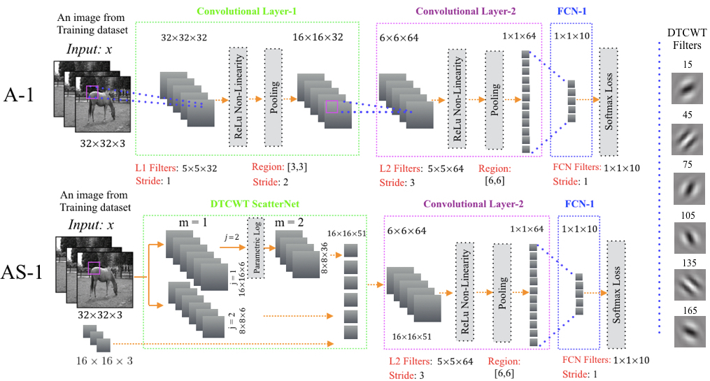
This paper proposes the DTCWT ScatterNet Convolutional Neural Network (DTSCNN) formed by replacing the first convolutional, relu and pooling layers of the CNN with a two-layer parametric log based DTCWT ScatterNet [27]. This extracts relatively symmetric translation invariant representations from a multi-resolution image using the dual-tree complex wavelet transform (DTCWT) [12] and a parametric log transformation layer. These extracted features, that incorporate edge information similar to the first layers of the networks trained on ImageNet [31], [10], are used by the middle and later CNN layers to learn high-level features. This helps the proposed DTSCNN architecture to converge faster as it has fewer filter weights to learn compared to its corresponding CNN architecture (Section 2). In addition, the CNN layers can learn more complex patterns from the start of learning as it is not necessary to wait for the first layer to learn edges as they are already extracted by the ScatterNet.
The performance of the DTSCNN architecture is evaluated on (i) Classification error and, (ii) Computational efficiency and the rate of learning with over 50 experiments performed with 14 CNN architectures. The efficient learning of the DSTCNN architectures is demonstrated by their ability to train faster and with lower classification error on small as well as large training datasets, generated from the CIFAR-10 dataset. The DTCWT ScatterNet front-end is also shown to give similar performance to the first convolutional pre-trained layers of CNNs which capture problem specific filter representations, on Caltech-101 as well as CIFAR-10 datasets. A comparison with the state-of-the-art is also presented on both datasets.
The paper is divided into the following sections. Section 2 presents the parametric log based DTCWT ScatterNet Convolutional Neural Network (DTSCNN). Section 3 presents the experimental results while Section 4 draws conclusions.
2 Proposed DTSCNN Network
This section details the proposed DTCWT ScatterNet Convolutional Neural Network (DTSCNN) composed by combining the two-layer parametric log based DTCWT ScatterNet with the later layers (middle and back-end) of the CNN to perform object classification. The ScatterNet (front-end) is first briefly explained followed by the details regarding the (back-end) CNN architecture.
The parametric log based DTCWT ScatterNet [27] is an improved version (both on classification error and computational efficiency) of the multi-layer Scattering Networks [4, 19, 26, 18, 5] that extracts relatively symmetric translation invariant representations from a multi-resolution image using the dual-tree complex wavelet transform (DTCWT) [12] and parametric log transformation layer. This network extracts feature maps that are denser over scale from multi-resolution images at 1.5 times and twice the size of the input image. Below we present the formulation of the parametric DTCWT ScatterNet for a single input image which may then be applied to each of the multi-resolution images.
| Architecture | Layers | ||||||||||
|---|---|---|---|---|---|---|---|---|---|---|---|
| L1-F | PL1-R | L2-F | PL2-R | L3-F | PL3-R | L4-F | L5-F | FCN1 | FCN2 | FCN3 | |
| a,b | [c,c] | a,b | [c,c] | a,b | [c,c] | a,b | a,b | a,b | a,b | a,b | |
| A-1 | 5,32 | [3,3] | 5,64 | [6,6] | – | – | – | – | 1,10 | – | – |
| A-2 | 5,32 | [3,3] | 5,32 | [6,6] | 5,64 | [4,4] | – | – | 1,32 | 1,10 | – |
| A-3 | 5,32 | [3,3] | 5,32 | [3,3] | 5,64 | [3,3] | 4,64 | – | 1,32 | 1,16 | 1,10 |
| A-4 | 5,32 | [3,3] | 5,32 | [3,3] | 5,64 | – | 4,64 | 4,64 | 1,32 | 1,16 | 1,10 |
| Training Data Sample Size | 300 | 500 | 1000 | 2000 | 5000 | 10000 | 25000 | 50000 |
|---|---|---|---|---|---|---|---|---|
| Batch Size | 5 | 5 | 10 | 20 | 50 | 100 | 100 | 100 |
The invariant features are obtained at the first layer by filtering the input signal with dual-tree complex wavelets at different scales () and six pre-defined orientations () fixed to and . To build a more translation invariant representation, a point-wise non-linearity (complex modulus) is applied to the real and imaginary part of the filtered signal:
| (1) |
The parametric log transformation layer is then applied to all the oriented representations extracted at the first scale with a parameter , to reduce the effect of outliers by introducing relative symmetry of pdf, as shown below:
| (2) |
Next, a local average is computed on the envelope that aggregates the coefficients to build the desired translation-invariant representation:
| (3) |
The high frequency components lost due to smoothing are retrieved by cascaded wavelet filtering performed at the second layer. The retrieved components are again not translation invariant so invariance is achieved by first applying the L2 non-linearity of eq(2) to obtain the regular envelope:
| (4) |
and then a local-smoothing operator is applied to the regular envelope () to obtain the desired second layer () coefficients with improved invariance:
| (5) |
The scattering coefficients for each layer are:
| (6) |
| Architectures | Classification Error | |||||||
|---|---|---|---|---|---|---|---|---|
| Derived from LeNet [15] | Training Data Sample Size | |||||||
| 300 | 500 | 1000 | 2000 | 5000 | 10000 | 25000 | 50000 | |
| A-1: 2Conv-1FCon | 77.8 | 73.2 | 70.3 | 66.7 | 61.3 | 54.9 | 45.3 | \cellcolorgray!5038.1 |
| AS-1: DTS-1Conv-1FCon | \cellcolorgray!5069.4 | \cellcolorgray!5065.8 | \cellcolorgray!5060.1 | \cellcolorgray!5058.9 | \cellcolorgray!5052.7 | \cellcolorgray!5054.7 | \cellcolorgray!5040.4 | 38.7 |
| A-2: 3Conv-2FCon | 66.8 | 62.0 | 57.5 | 52.8 | 46.1 | 40.1 | \cellcolorgray!5032.7 | \cellcolorgray!5027.3 |
| AS-2: DTS-2Conv-2FCon | \cellcolorgray!5063.7 | \cellcolorgray!5055.1 | \cellcolorgray!5049.5 | \cellcolorgray!5043.7 | \cellcolorgray!5039.1 | \cellcolorgray!5040.0 | 33.8 | 28.3 |
| A-3: 4Conv-3FCon | 62.2 | 57.4 | 51.0 | 46.8 | 40.1 | 35.1 | 29.2 | 24.2 |
| AS-3:DTS-3Conv-3FCon | \cellcolorgray!5056.8 | \cellcolorgray!5054.9 | \cellcolorgray!5050.9 | \cellcolorgray!5045.3 | \cellcolorgray!5039.7 | \cellcolorgray!5034.9 | \cellcolorgray!5028.7 | \cellcolorgray!5024.1 |
| A-4: 5Conv-3FCon | \cellcolorgray!5058.4 | 54.4 | 47.4 | 41.8 | \cellcolorgray!5035.0 | 32.2 | 25.7 | 22.1 |
| AS-4: DTS-4Conv-3FCon | 59.8 | \cellcolorgray!5054.0 | \cellcolorgray!5047.3 | \cellcolorgray!5041.3 | 38.4 | \cellcolorgray!5031.8 | \cellcolorgray!5025.2 | \cellcolorgray!5022.0 |
| Standard Deep Architectures | Training Data Sample Size | |||||||
| A-5: NIN [16] | 89.2 | 84.4 | 45.5 | 34.9 | 27.1 | 18.8 | \cellcolorgray!5013.3 | \cellcolorgray!508.1 |
| AS-5: DTS-NIN | \cellcolorgray!5083.2 | \cellcolorgray!5080.1 | \cellcolorgray!5041.0 | \cellcolorgray!5032.2 | \cellcolorgray!5025.3 | \cellcolorgray!5018.4 | 13.4 | 8.2 |
| A-6: VGG [25] | 89.9 | 89.7 | 89.1 | 59.6 | 36.6 | 28 | 16.9 | \cellcolorgray!507.5 |
| AS-6: DTS-VGG | \cellcolorgray!5083.5 | \cellcolorgray!5082.8 | \cellcolorgray!5081.6 | \cellcolorgray!5056.7 | \cellcolorgray!5034.9 | \cellcolorgray!5027.2 | \cellcolorgray!5016.9 | 7.6 |
| A-7: WResNet [30] | 87.2 | 53.2 | 43.2 | 31.1 | 18.8 | 13.6 | 10.1 | 3.6 |
| AS-7: DTS-WResNet | \cellcolorgray!5081.2 | \cellcolorgray!5049.8 | \cellcolorgray!5041.2 | \cellcolorgray!5030.1 | \cellcolorgray!5018.6 | \cellcolorgray!5013.5 | \cellcolorgray!509.9 | \cellcolorgray!503.6 |
Next, the proposed DTSCNN architectures (AS1 to AS4) are realized by replacing the first convolutional layer of the A-1 to A-4 CNN architectures with the ScatterNet (described above), as shown in Fig. 1. The four CNN architectures (A-1 to A-4, shown in Table. 1) are derived from the LeNet [15] architecture because they are relatively easy to train due to its small memory footprint. In addition to the derived architectures, the DTSCNN is also realized by using ScatterNet as the front-end of three standard deep architectures namely; Network in Network (NIN) [16] (A-5), VGG [25] (A-6), and wide ResNet [30] (WResNet) (A-7). The DTSCNN architectures (AS-5, AS-6, AS-7) for the standard architectures (NIN (A-5), VGG (A-6), WResNet (A-7)) are again obtained by removing the first convolutional layer of each network and replacing it with the ScatterNet. The architectures are trained in an end-to-end manner by Stochastic Gradient Descent with softmax loss until convergence.
3 Experimental Results
The performance of the DTSCNN architecture is demonstrated on CIFAR-10 and Caltech-101 datasets with over 50 experiments performed with 14 CNN architectures of increasing depth on (i) Classification error and, (ii) Computational efficiency and the rate of learning. The generic nature of the features extracted by the DTCWT ScatterNet is shown by an equivalent performance to the pre-trained CNN front-ends. The details of the datasets and the results are presented below.
3.1 Datasets
The CIFAR-10 [13] dataset contains a total of 50000 training and 10000 test images of size . The efficient learning of the proposed DTSCNN network is measured on 8 training datasets of sizes: 300, 500, 1000, 2000, 5000, 10000, 25000 and 50000 images generated randomly by selecting the required number of images from the full 50000 training dataset. It is made sure that an equal number of images per object class are sampled from the full training dataset. For example, a training dataset sample size of 300 will include 30 images per class. The full test set of 10000 images is used for all the experiments.
Caltech-101 [9] dataset contains 9K images each of size 224224 labeled into 101 object categories and a background class. The classification error on this dataset is measured on 3 randomly generated splits of training and test data, so that each split contains 30 training images per class, and up to 50 test images per class. In each split, 20% of training images were used as a validation set for hyper-parameter selection. Transfer learning is used to initialize the filter weights for the networks that are used to classify this dataset because the number of training samples are not sufficient to train the networks from a random start.
3.2 Evaluation and Comparison on Classification Error
The classification error is recorded for the proposed DTSCNN architectures and compared with the derived (A-1 to A-4) as well as the standard (A-5 to A-7) CNN architectures, for different training sample sizes, as shown in Table. 1. The parameters used to train the CNN architectures are shown in Table. 2. The classification error corresponds to the average error computed for 5 repetitions.
It can be observed from Table. 3 that the difference in classification error for the derived CNN architectures (A-1 to A-4) is at around 9% for the small training datasets with 1000 training images. This difference in error reduces with the increase in the size of the training dataset and with increase in the depth of the architectures as shown in Table. 3. In fact, the deeper CNN architectures such 5CV-3FCN (A-4) outperformed their corresponding DTSCNN architectures by a small margin.
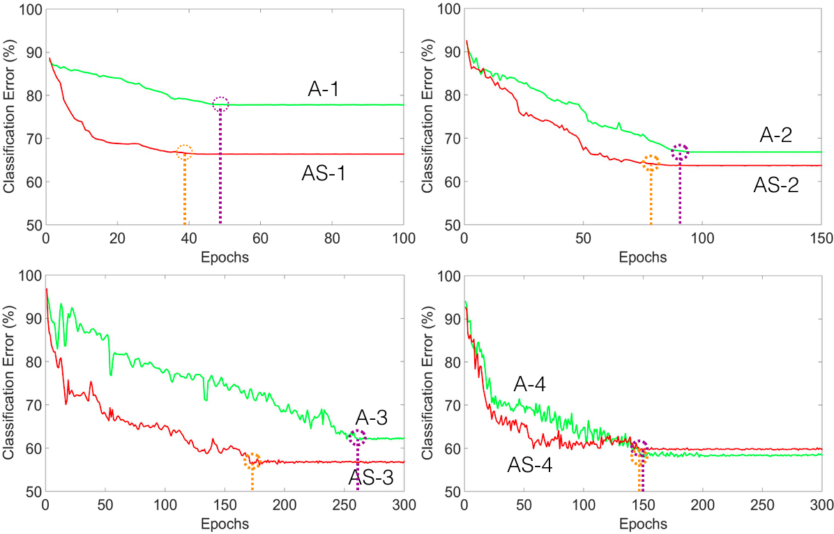
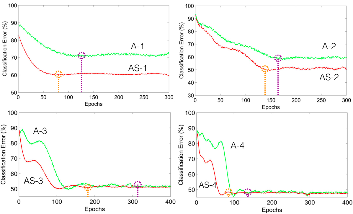
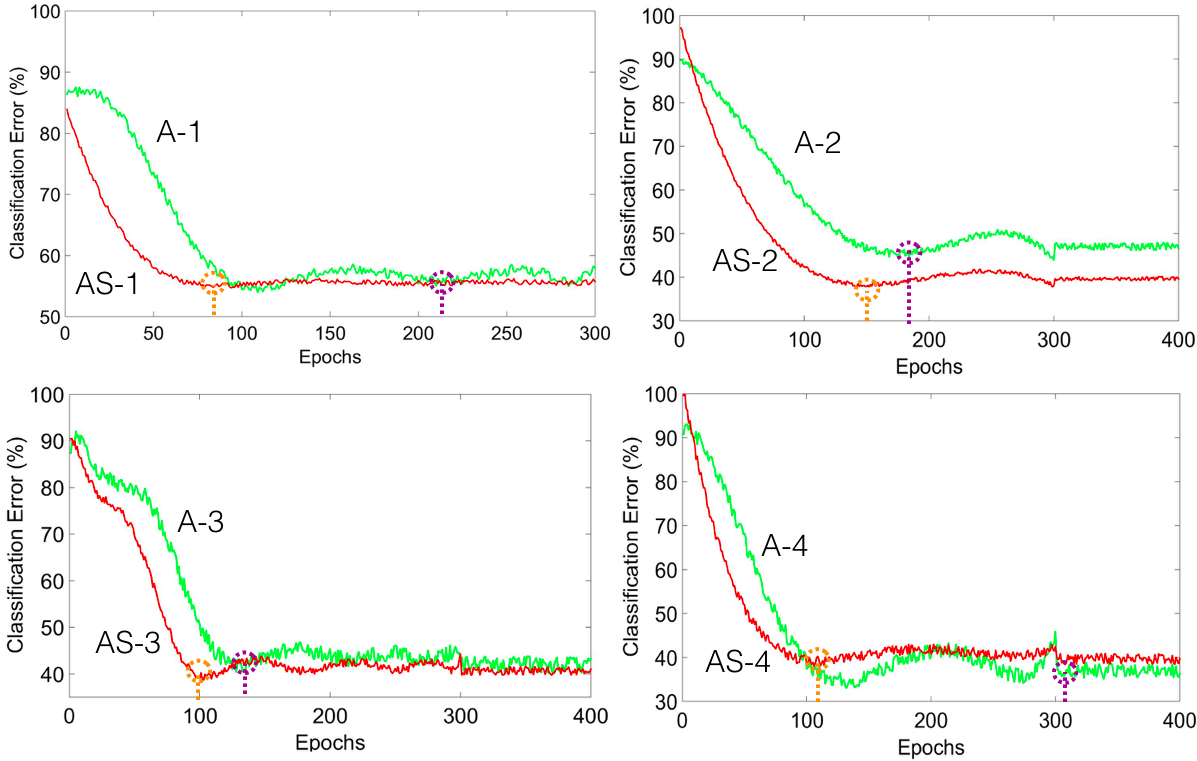
A similar trend in classification error is also observed for the standard more deeper CNN architectures (A-5 to A-7). The difference in classification error is large between the DTSCNN (AS-5 to AS-7) and the original (A-5 to A-7), architectures for small training datasets while both class of architectures produce a similar classification error for datasets with large training size. In fact, the wide ResNet (WResNet) (A-7) and its corresponding DTSCNN architecture (AS-7) result in the same classification error of 3.6%.


3.3 Analysis on Computational Efficiency and Learning
This section compares the efficient and faster learning of the proposed DTSCNN architectures against the CNN architectures (A-1 to A-4) derived from LeNet [15] as well as the standard (A-5 to A-7) deep learning architectures for a range of small and large training dataset sizes.
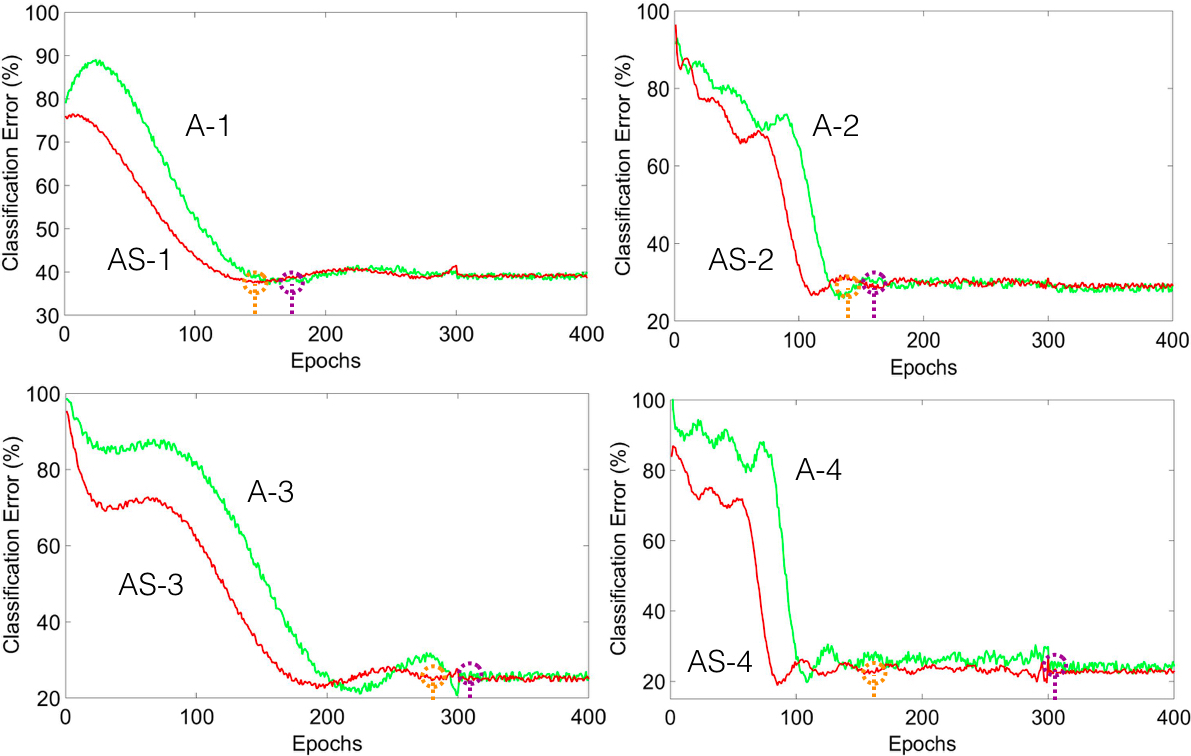
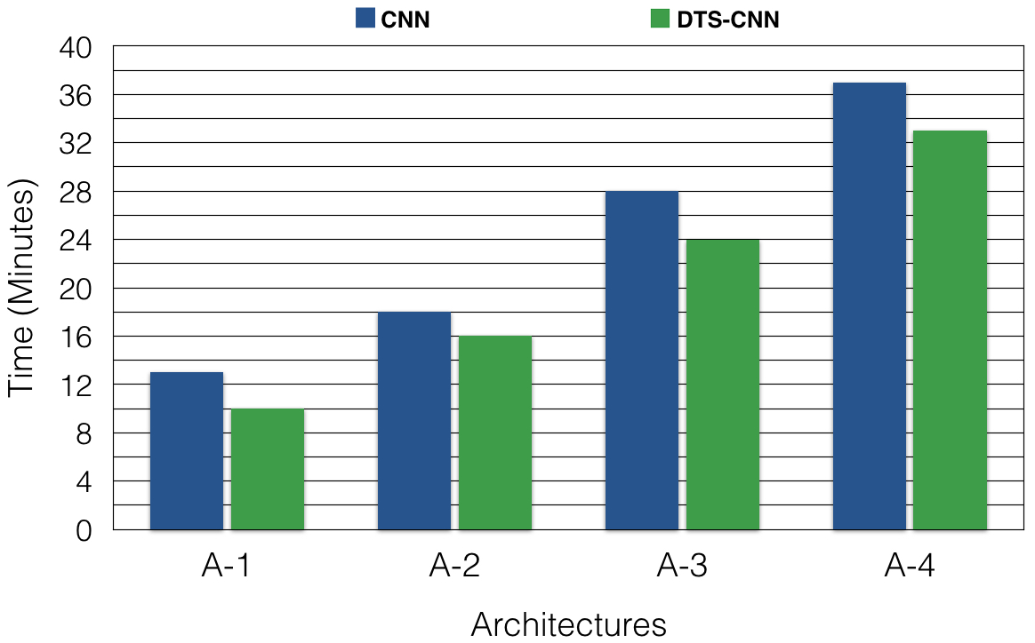
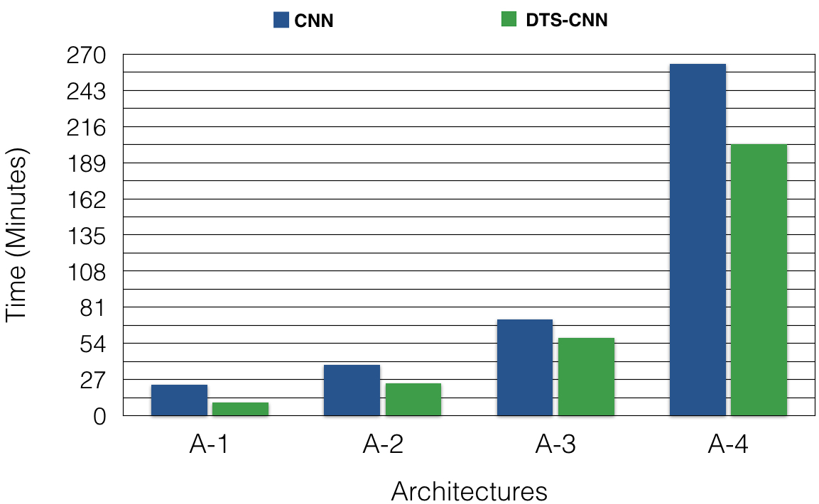
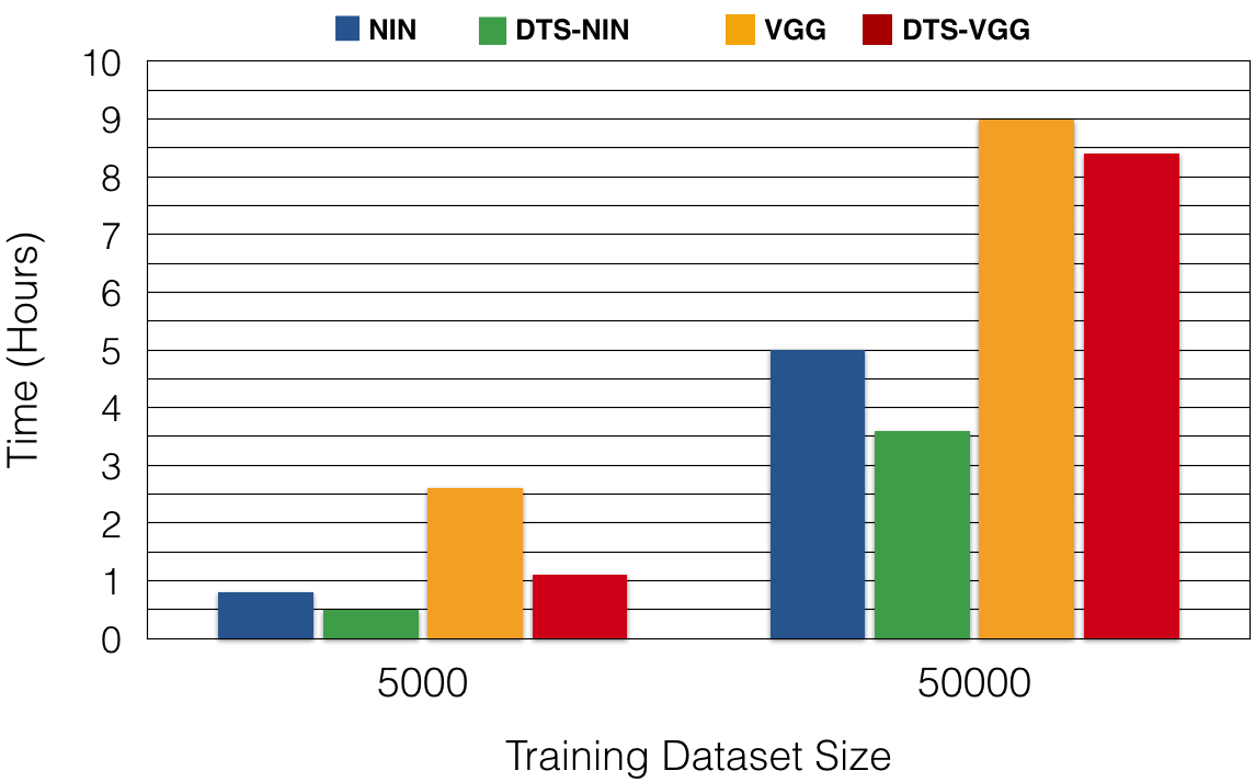
The DTSCNN architectures have a higher rate of learning or faster converge than the original CNN architectures because the numbers of filter weights required to be learned are smaller but also because the ScatterNet extracts edge representations that allow the later CNN layers to learn high-level features from the first epoch onwards. The faster convergence is shown for both the derived (A-1 to A-4) and standard deep architectures (A-5 to A-7) as shown in Fig. 2 and Fig. 3, respectively. An architecture is considered to have converged at a specific epoch when the error value for the subsequent epochs changes within 2% of the error value at that specific epoch. The convergence is marked on the epoch axis using an orange dotted line for the DTSCNN architecture and a purple dotted line for the CNN architectures. As observed from Fig. 2 and Fig. 3, the orange line has a lower epoch value as compared to the purple line indicating the faster convergence.
The time required for training the original and their corresponding DSTCNN architectures is presented for a small (5000) and large training dataset (50000) for both the derived (A-1 to A-4) and standard deep architectures (A-5 to A-6), as shown in Fig. 2 and Fig. 3, respectively. The time for convergence is again measured to within 2% of the final converged error value. As observed from both figures, the training time is higher for the original networks than the DTSCNN networks because of the reasons mentioned above.
The networks are trained using the MatConvNet [29] package on a server with a NVIDIA GeForce 7800 GTX card.
3.4 Comparison with Pre-trained CNN First Layers
The classification performance of the DTCWT ScatterNet front-end is compared with the first pre-trained convolutional layer for the Network in Network (NIN) [16] and the Visual Geometry Group convolutional (VGG) [25] architectures, on Caltech-101 and CIFAR-10 datasets. The filter weights for both the NIN and the VGG networks are initialized with the weights obtained from their models pre-trained on ImageNet (found here [1]). The first layers for both the architectures are fixed to be the ScatterNet and the pre-trained convolutional layer, while the filter weights only in later layers are fine-tuned using the training images of CIFAR-10 and Caltech-101. The ScatterNet front-end gives similar performance to the pre-trained first convolutional layer on classification error for both datasets as shown in Table. 4. For this experiment, dropout, batch normalization and data augmentation with crops and horizontal flips were utilized [2]. The use of the NIN network is preferred as it gives similar performance to the VGG network while being 4 times faster.
| Dataset | State-of-the-art Architectures | |||
|---|---|---|---|---|
| T-NIN | DTS-NIN | T-VGG | DTS-VGG | |
| Caltech-101 | 12.3 | \cellcolorgray!5012.26 | \cellcolorgray!508.78 | 9.23 |
| CIFAR-10 | \cellcolorgray!508.25 | 8.34 | \cellcolorgray!508.31 | 9.02 |
3.5 Comparison with the state-of-the-art
This section compares the architectures that produced the best classification performance with the state-of-the-art on CIFAR-10 and Caltech-101. The DTS-WResNet (AS-7) and DTS-VGG (AS-6) resulted in the best classification performance on CIFAR-10 and Caltech-101 with 3.6% and 8.08% classification error, respectively.
The DTS-WResNet (AS-7) architecture is compared with the state-of-the-art CNN architectures on CIFAR-10. DTS-WResNet outperformed these architectures as shown in Table 5.
| Dataset | State-of-the-art Architectures | |||||
|---|---|---|---|---|---|---|
| DW | VGG | E-CNN | NIN | DSN | MON | |
| Cifar-10 | \cellcolorgray!503.6 | 7.5 | 8.0 | 8.1 | 8.2 | 9.3 |
Next, the DTS-VGG (AS-6) architecture is compared against the state-of-the-art CNN architectures for the Caltech-101 dataset. On this dataset, the DTS-VGG outperformed some of the architectures while produced a marginally lower classification performance for others (Table 6).
| Dataset | State-of-the-art Architectures | |||||
|---|---|---|---|---|---|---|
| DV | SPP | VGG | E-CNN | EP | ZF | |
| Caltech-101 | 8.78 | \cellcolorgray!506.6 | 7.3 | 8.5 | 12.2 | 13.5 |
4 Conclusion
The proposed DTSCNN architectures, when trained from scratch, outperforms the corresponding original CNN architectures on small datasets by a useful margin. For larger training datasets, the proposed networks give similar error compared to the original architectures. Faster rate of convergence is observed in both cases for shallow as well as deep architectures.
The DTCWT scattering front-end is mathematically designed to deal with all edge orientations equally and with 2 or more scales, as required. The generic nature of the DTCWT scattering front-end is shown by its similar classification performance to the front-end of learned networks, on two different datasets. The generic features are likely to give it wide applicability to both small and large image datasets as it gives lower (small dataset) or similar classification error (large dataset), with faster rates of convergence.
Future work includes extending the DTCWT Scattering Network front-end for other learning frameworks, with a view to improving learning rates further.
References
- [1] https://github.com/bvlc/caffe/wiki/model-zoo.
- [2] http://torch.ch/blog/2015/07/30/cifar.html. 2015.
- [3] H. at al. Spatial pyramid pooling in deep convolutional networks for visual recognition. ArXiv:1406.4729v2, 2014.
- [4] J. Bruna and S. Mallat. Invariant scattering convolution networks. IEEE Transaction on Pattern Analysis and Machine Intelligence, 35:1872 –1886, 2013.
- [5] F. Cotter and N. Kingsbury. Visualizing and improving scattering networks. Axiv, 2017.
- [6] A. D. et al. Discriminative unsupervised feature learning with exemplar convolutional neural networks. ArXiv:1406.6909, 2014.
- [7] C. L. et al. Deeply-supervised nets. ArXiv:1409.5185, 2014.
- [8] I. G. et al. Maxout networks. ICML, 2013.
- [9] L. Fei-Fei, R. Fergus, and P. Perona. Learning generative visual models from few training examples: an incremental bayesian approach tested on 101 object categories. IEEE. CVPR Workshop on Generative-Model Based Vision, 2004.
- [10] R. Girshick, J. Donahue, T. Darrell, and J. Malik. Rich feature hierarchies for accurate object detection and se- mantic segmentation. arXiv:1311.2524, 2013.
- [11] S. Jain, S. Gupta, and A. Singh. A novel method to improve model fitting for stock market prediction. International Journal of Research in Business and Technology, 3(1), 2013.
- [12] N. Kingsbury. Complex wavelets for shift invariant analysis and filtering of signals. Applied and computational harmonic analysis, 10:234–253, 2001.
- [13] A. Krizhevsky and G. Hinton. Learning multiple layers of features from tiny images. 2009.
- [14] A. Krizhevsky, I. Sutskever, and G. Hinton. Imagenet classification with deep convolutional neural networks. NIPS, 2012.
- [15] Y. LeCun, L. Bottou, Y. Bengio, and P. Haffner. Gradient-based learning applied to document recognition. Proceedings of the IEEE, 86(11):2278–2324, 1998.
- [16] M. Lin, Q. Chen, and S. Yan. Network in network. arXiv:1312.4400, 2013.
- [17] R. Mao, H. Zhu, L. Zhang, and A. Chen. A new method to assist small data set neural network learning. Proceeding of the sixth International Conference on Intelligent Systems Design and Applications, pages 17–22, 2006.
- [18] S. Nadella, A. Singh, and S. Omkar. Aerial scene understanding using deep wavelet scattering network and conditional random field. European Conference on Computer Vision (ECCV) workshops, 9913:205–214, 2016.
- [19] E. Oyallon and S. Mallat. Deep roto-translation scattering for object classification. IEEE Conference on Computer Vision and Pattern Recognition, pages 2865–2873, 2015.
- [20] G. Papandreou. Deep epitomic convolutional neural networks. ArXiv:1406.6909, 2014.
- [21] A. Pasini. Artificial neural networks for small dataset analysis. Journal of Thoracic Disease, 7(11):2278–2324, 2015.
- [22] J. Plaza, A. Plaza, R. Perez, and P. Martinez. On the use of small training sets for neural network-based characterization of mixed pixels in remotely sensed hyperspectral images. Pattern Recognition, 42:3032–3045, 2009.
- [23] R. Raina, A. Battle, H. Lee, B. Packer, and A. Y. Ng. Self-taught learning: Transfer learning from unlabeled data. 24th International Conference on Machine Learning, pages 759–766, 2007.
- [24] A. Razavian, H. Azizpour, J. Sullivan, and S. Carlsson. Cnn features off-the-shelf: an astounding baseline for recognition. IEEE conference on Computer Vision and Pattern Recognition, pages 512–519, 2014.
- [25] K. Simonyan and A. Zisserman. Very deep convolutional networks for large-scale image recognition. International conference on learning representation, 2015.
- [26] A. Singh and N. Kingsbury. Multi-resolution dual-tree wavelet scattering network for signal classification. 11th International Conference on Mathematics in Signal Processing, 2016.
- [27] A. Singh and N. Kingsbury. Dual-tree wavelet scattering network with parametric log transformation for object classification. In IEEE International Conference on Acoustics, Speech and Signal Processing (ICASSP), pages 2622–2626, 2017.
- [28] A. Toshev and C. Szegedy. Deeppose: Human pose estimation via deep neural networks. CoRR, abs/1312.4659, 2013.
- [29] A. Vedaldi and K. Lenc. Matconvnet. University of Oxford, 2015.
- [30] S. Zagoruyko and N. Komodakis. Wide residual networks. ArXiv:1605.07146, 2016.
- [31] M. Zeiler and R. Fergus. Visualizing and understanding convolutional neural networks. arXiv:1311.2901, 2013.
- [32] M. D. Zeiler and R. Fergus. Visualizing and understanding convolutional networks. ECCV, 2014.
- [33] X. Zhang, Y. Fu, S. Jiang, L. Sigal, and G. Agam. Learning from synthetic data using a stacked multichannel autoencoder. Axiv:1509.05463, 2015.