Testing the consistency of three-point halo clustering in Fourier and configuration space

Abstract

We compare reduced three-point correlations $Q$ of matter, haloes (as proxies for galaxies) and their cross correlations, measured in a total simulated volume of $\sim 100\ (h^{-1}\text{Gpc})^{3}$, to predictions from leading order perturbation theory on a large range of scales in configuration space. Predictions for haloes are based on the non-local bias model, employing linear ($b_{1}$) and non-linear ($c_{2}$, $g_{2}$) bias parameters, which have been constrained previously from the bispectrum in Fourier space. We also study predictions from two other bias models, one local ($g_{2}=0$) and one in which $c_{2}$ and $g_{2}$ are determined by $b_{1}$ via approximately universal relations. Overall, measurements and predictions agree when $Q$ is derived for triangles with $(r_{1}r_{2}r_{3})^{1/3}\gtrsim 60h^{-1}\text{Mpc}$, where $r_{1-3}$ are the sizes of the triangle legs. Predictions for $Q_{matter}$, based on the linear power spectrum, show significant deviations from the measurements at the BAO scale (given our small measurement errors), which strongly decrease when adding a damping term or using the non-linear power spectrum, as expected. Predictions for $Q_{halo}$ agree best with measurements at large scales when considering non-local contributions. The universal bias model works well for haloes and might therefore be also useful for tightening constraints on $b_{1}$ from $Q$ in galaxy surveys. Such constraints are independent of the amplitude of matter density fluctuation ($\sigma_{8}$) and hence break the degeneracy between $b_{1}$ and $\sigma_{8}$, present in galaxy two-point correlations.

1 Introduction

Higher-order correlations, induced by gravity into the distribution of large-scale matter density fluctuations, contain information which cannot be captured by second-order statistics. This information can be used to tighten constraints on cosmological models, as well as on models of galaxy formation. A key tool for obtaining such constraints are galaxy bias models (e.g. Desjacques et al., 2016). These models relate the density and the tidal field of the full matter content in a given region to the density of observable tracers, such as galaxies. They include a number of so-called bias parameters, which depend on the various processes that drive the tracer formation. Since these highly complex processes are only partly understood, the bias parameters cannot be predicted in a reliable way (e.g. Li et al., 2007; Müller et al., 2011; Pujol et al., 2017; Springel et al., 2017) and hence need to be measured from the data. Such measurements can be obtained from the analysis of weak gravitational lensing signals, or redshift space distortions. However, these methods rely on good redshift estimations and imaging of the tracers (i.e. galaxies) as well as on various model assumptions. It is therefore interesting to obtain independent measurements of the bias parameters, which is possible with a joint analysis of second- and third-order statistics. This approach becomes increasingly interesting as errors on these statistics decrease with the increasing volumes of upcoming galaxy surveys. Going to third-order in the statistical analysis of galaxy surveys does not only deliver bias measurements, but also measurements of the growth of matter fluctuations. The latter provide the aforementioned cosmological constraints, while the bias can be used to predict the number of galaxies per halo, which places constraints on galaxy formation models (e.g. Scoccimarro et al., 2001; Berlind & Weinberg, 2002; Cooray & Sheth, 2002).

The most general third-order statistics is the three-point correlation function (hereafter referred to as 3PCF), which is defined in configurations space. Alternatively one can study its Fourier space counterpart, the bispectrum. These two statistics contain in principle the same information. However, their analyses implicate different limitations and challenges, which can affect the physical interpretation of the results. A main advantage of the bispectrum is that an analysis in Fourier space allows for a clear exclusion of high frequency modes in the density fluctuations, which are difficult to interpret theoretically due to their highly non-linear evolution. In configuration space, these high frequency modes contribute to the 3PCF in principle at all scales. In practice one therefore needs to restrict the analysis to large scales, where their contribution is negligible, lavishing a lot of valuable data. Another advantage of the bispectrum is that its covariance is diagonal for Gaussian density fluctuations. This approximation works well, even for evolved density fields, while deviations from Gaussianity can also be taken into account (Scoccimarro, 2000; Sefusatti et al., 2006; Chan & Blot, 2016). The covariance of the 3PCF on the other hand is not diagonal, even for Gaussian fluctuations, which makes the modeling more difficult (Srednicki, 1993; Slepian & Eisenstein, 2015; Byun et al., 2017; Gualdi et al., 2017). An additional difference in the analysis of the bispectrum and the 3PCF lies in the fact that the computation of the latter is more expensive. However, this aspect can be tackled by employing advanced algorithms and appropriate computational resources, as done in this work (see also, Barriga & Gaztañaga, 2002; McBride et al., 2011a; Jarvis, 2015; Slepian & Eisenstein, 2015, and references therein). Besides its disadvantages, there are some arguments which speak for the 3PCF. One of them is the fact that the amplitude of the 3PCF (but not its errors) is not affected by shot-noise, whereas the latter affects the bispectrum amplitude at all scales and hence needs to be modelled for correcting the measurements. In addition, an analysis in configuration space has the advantage that complicated survey masks can be easily taken into account in the analysis of observational data, while in Fourier space such masks impose complicated effects on the measured bispectrum, which are difficult to model (e.g. Scoccimarro, 2000). A more general consideration is that it is easier to interpret effects such as redshift space distortions or baryon acoustic oscillations (BAO) on the statistics in configuration space, since that is where the physical processes which cause these effects happen. Studies of third-order correlations in the literature usually focus on either Fourier or configuration space (e.g. McBride et al., 2011b; Marín et al., 2013; Gil-Marín et al., 2015). However, it is worthwhile studying both statistics and cross-check the results, since their different advantages and disadvantages are quite complementary.

In this work we will conduct such a cross-check for the first time. Our main interest thereby is to verify if and when the bias parameters, obtained from the bispectrum are consistent with those which affect the 3PCF in configuration space. Our approach is based on the analysis of Chan et al. (2012, hereafter referred to as CSS12). These authors measured the bias parameters of large-scale structure tracers in Fourier space from a set of N-body simulations, using a leading-order perturbative model of the bispectrum and restricting the analysis to large modes with wave numbers $k\leq 0.1\ h\text{Mpc}^{-1}$. The tracers in their analysis are dark-matter halos, while the same method for measuring the bias can be applied to any other type of tracers, such as galaxies or galaxy clusters. For our cross-check we use the same perturbative model together with the bias parameters of CSS12 to predict the halo 3PCF in configuration space. We then measure the latter in the same set of simulations to test the predictions. This allows us to verify if and when the bias parameters measured from third-order statistics in Fourier space also describe the corresponding statistics in configuration space. Simultaneously we test at which scales, redshifts and halo mass ranges the leading order perturbative modeling of the 3PCF is an appropriate approximation.

1.1 Bias models tested

The bias model relates the density fluctuations and the tidal field of matter in a certain region to the density fluctuations of its tracers. These fluctuations are defined with respect to the mean density as $\delta\equiv(\rho-\bar{\rho})/\bar{\rho}$. Since the leading order perturbative expansion of third-order statistics, on which we focus in this analysis, is quadratic, we use the quadratic non-local bias model,

$$\delta_{h}=b_{1}\biggl{\{}\delta_{m}+\frac{1}{2}[c_{2}(\delta_{m}^{2}-\langle\delta_{m}^{2}\rangle)+g_{2}\mathcal{G}_{2}]\biggr{\}}.$$ (1)

The indices $h$ and $m$ refer to the halo and matter density fluctuations respectively. The parameters $b_{1}$ and $c_{2}$ are hereafter referred to as local linear and quadratic bias (Fry & Gaztanaga, 1993), while $g_{2}$ will be referred to as quadratic non-local bias, since it scales with the tidal field term $\mathcal{G}_{2}$, which can be generated by masses outside of the volume in which $\delta_{g}$ is defined (see CSS12; McDonald & Roy, 2009; Baldauf et al., 2012). The term for the smoothed tidal field is given by a second-order Gallileon

$$\mathcal{G}_{2}({\bf r})=\int\beta_{12}\theta_{v}({\bf k}_{1})\theta_{v}({\bf k}_{2})\ \hat{W}[k_{12}R]e^{i{\bf k}_{12}\cdot{\bf r}}d^{3}{\bf k}_{1}d^{3}{\bf k}_{2},$$ (2)

where ${\bf k}_{i}$ and ${\bf k}_{12}\equiv{\bf k}_{2}-{\bf k}_{1}$ are wave vectors of density oscillations, $\beta_{12}\equiv 1-({\hat{\bf k}}_{1}\cdot{\hat{\bf k}}_{2})^{2}$ represents the mode-coupling between density oscillations which describes tidal forces, $\theta_{v}\equiv\nabla^{2}\Phi_{v}$ is the divergence of the normalised velocity field (${\bf v}/\mathcal{H}/f$) and $\hat{W}[k_{12}R]$ is the window function in Fourier space (CSS12). Note that the non-local bias has also been referred to as an additional local bias parameter, since the tidal field is a local observable, which depends on derivatives of the potential (see CSS12, Desjacques et al., 2016). However, in this work we call it non-local, since it is non-local in the density.

We use three sets of bias parametrizations for predicting the 3PCF. The first set consists of the bias parameters $b_{1}$, $c_{2}\equiv b_{2}/b_{1}$ and $g_{2}\equiv 2\gamma_{2}/b_{1}$, obtained by CSS12 from fitting the non-local bias model predictions for the bispectrum at leading order to measurements in the same set of simulations as studied in this work. Here $b_{2}$ and $\gamma_{2}$ are the quadratic local and the non-local bias parameters respectively, in the notation of CSS12. The second set equals the first set, except for the non-local bias parameter $g_{2}$, which is set to zero in order to verify the impact of the non-local contributions on the 3PCF predictions. In the third set the linear bias $b_{1}$ is the only input parameter. This is the same parameter, as in the two previous sets, but was obtained by CSS12 from fits of the linear bias model ($\delta_{h}=b_{1}\delta_{m}$) to the power spectrum. The quadratic local bias parameter $c_{2}$ in this third set is computed from the (approximately) universal relation $c_{2}\simeq 0.77b_{1}^{-1}-2.43+b_{1}$ , given by Hoffmann et al. (2017) (see also Hoffmann et al., 2015b; Lazeyras et al., 2016, for similar relations). The non-local bias in the third set is obtained from the local Lagrangian model, $g_{2}=-(4/7)(1-1/b_{1})$. The three sets of bias model parameters are summarised in Table 1 and will in the following be referred to as non-local, local and $b_{\delta^{2}fix}$ model respectively.

Table 1: Different bias models studied in this work. The bias parameters have been measured in Fourier space from the same set of simulations by CSS12. For the $b_{\delta^{2}fix}$ model we use a roughly universal relation for the quadratic local bias $c_{2}(b_{1})$ (Hoffmann et al., 2017) and the local Lagrangian model for the quadratic non-local $g_{2}(b_{1})$.

bias model	description
non-local	$b_{1}$, $c_{2}$, $g_{2}$ from bispectrum fits
local	same $b_{1}$ and $c_{2}$ as above, $g_{2}=0$
$b_{\delta^{2}fix}$	$b_{1}$ from power spectrum fits,
	$c_{2}=0.77b_{1}^{-1}-2.43+b_{1}$,
	$g_{2}=-(4/7)(1-1/b_{1})$

For a three-dimensional analysis of real spectroscopic surveys one would further need to take into account redshift space distortions in the modeling. Redshift space distortions cancel out approximately at large scales in the reduced 3PCF (defined in Section 2.1, see e.g. Gaztañaga & Scoccimarro, 2005), but there are non-linear contributions that could be as large as the non-local terms. There is some indication in simulations that non-local terms can cancel out with redshift space distortions, (e.g. Fig.17 in Hoffmann et al., 2015a), but this requires further study. Large volume photometric surveys, such as DES or LSST will provide additional constraints from weak lensing of the projected 3PCF, both of galaxy and matter correlations, as well as galaxy-matter cross-correlations. Since those surveys measure redshifts from broad-band photometry these probes will have little contamination by redshift space distortions. All this is beyond the scope of this paper, but should be a clear continuation of our study.

2 Three-point correlations $Q$

2.1 Definitions

Our 3PCF analysis is applied on density fields $\rho^{x}(\bf r)$, where $x$ refers to the density of matter ($x=m$) or of its tracers, such as galaxies or, as in our case, dark matter halos ($x=h$) at the position $\bf r$. The density fields are smoothed with a top-hat filter of scale $R$ and described by the normalised density fluctuations $\delta^{x}({\bf r}_{i})\equiv\delta^{x}_{i}$, introduced in Section 1.1. Note that, in contrast to the notation in equation (1), we now set $x$ as upper index to avoid confusion between the position and the power indices in the following. The 3PCF can be defined as the average product of density fluctuations at three positions $({\bf r}_{1},{\bf r}_{2},{\bf r}_{3})$, which form a triangle. In the case of the halo-matter-matter cross-correlations it is written as

$$\zeta^{hmm}(r_{12},r_{13},r_{23})\equiv\langle\delta^{h}_{1}\delta^{m}_{2}\delta^{m}_{3}\rangle(r_{12},r_{13},r_{23}),$$ (3)

where $r_{ij}\equiv|{\bf r}_{i}-{\bf r}_{j}|$ are the absolute values of the triangle legs and $\langle\ldots\rangle$ denotes the average over all possible triangle orientations and translations. We proceed by defining the symmetric reduced three-point cross-correlation,

$$Q_{\times}\equiv\\ \frac{1}{3}\frac{\zeta^{hmm}+\zeta^{mhm}+\zeta^{mmh}}{\zeta^{\times}_{H}}$$ (4)

and drop the expression reduced in the following. The hierarchical three-point cross-correlation in the denominator, defined as

$$\zeta^{\times}_{H}\equiv\xi^{hm}_{12}\xi^{hm}_{13}+\xi^{hm}_{12}\xi^{hm}_{23}+\xi^{hm}_{13}\xi^{hm}_{23},$$ (5)

is comprised of two-point cross-correlations $\xi_{ij}^{xy}\equiv\langle\delta^{x}_{i}\delta^{y}_{j}\rangle(r_{ij})$ between the density fields $x$ and $y$ (e.g. Peebles & Groth, 1975; Fry, 1984). The corresponding expressions for the three-point auto correlations for matter and halos, ($Q_{m}$ and $Q_{h}$ respectively) are defined analogously, i.e. $Q_{m}\equiv\zeta^{mmm}/\zeta_{H}^{mmm}$ and $Q_{h}\equiv\zeta^{hhh}/\zeta_{H}^{hhh}$.

2.2 Modeling

Our predictions for $Q_{h}$ and $Q_{\times}$ are based on the non-local quadratic bias model from equation (1), which yields at leading-order perturbative expansion in terms of $\delta_{m}$

$$Q_{h}\simeq\frac{1}{b_{1}}[Q_{m}+c_{2}+g_{2}Q_{nloc}],$$ (6)

where $b_{1}$ and $c_{2}$ are the local linear and quadratic bias parameters respectively. The non-local contribution $Q_{nloc}$ scales with the non-local quadratic bias parameter $g_{2}$ (see CSS12; Baldauf et al., 2012). The corresponding leading order expression for the halo-matter-matter cross-correlation is given by

$$Q_{\times}\simeq\frac{1}{b_{1}}[Q_{m}+\frac{1}{3}(c_{2}+g_{2}Q_{nloc})].$$ (7)

Equation (6) has an important application in the analysis of galaxy surveys, since it allows for bias measurements which are independent of the linear growth of matter fluctuations (e.g. Frieman & Gaztanaga, 1994; Sefusatti et al., 2006; McBride et al., 2011b; Marín et al., 2013; Gil-Marín et al., 2015) and hence breaks the growth-bias degeneracy. However, cosmological constraints from such bias measurements are limited by the inaccuracies of the $Q_{h}$ modeling as explained in the following.

The statistics of the full matter field, $Q_{m}$ and $Q_{nloc}$, cannot be observed in galaxy surveys and hence need to be predicted for a given cosmology. $Q_{m}$ is therefore often predicted from N-body simulations. This approach has also been used by CSS12 for measuring the bias parameters in their simulations, as it captures the non-linear contributions to $Q_{m}$. However, these authors employ an analytical expression for the quadratic non-local contribution $Q_{nloc}$, which is in Fourier space simply related to the cosine of the angle between two wave vectors. Direct measurements of $Q_{nloc}$ would be more complicated (see Section 3.2). Another disadvantage of deriving the $Q_{m}$ and $Q_{nloc}$ from simulations, is that a dense sampling of the cosmological parameter space for deriving constraints from observations would require enormous resources (albeit $Q_{m}$ and $Q_{nloc}$ are independent of the linear growth factor and hence only weakly depend on cosmology at large scales). In this analysis we will therefore employ predictions from leading order perturbation theory for $Q_{m}$ and $Q_{nloc}$ (Jing & Boerner, 1997; Gaztanaga & Bernardeau, 1998; Barriga & Gaztañaga, 2002; Bel et al., 2015). These leading order approximations, as well as those of $Q_{h}$ and $Q_{\times}$ in equation (6) and (7) introduce inaccuracies in the modeling, in particular at small triangle scales, which are strongly affected by high frequency, non-linear modes (Scoccimarro et al., 1998; Pollack et al., 2012).

Measurements of the different 3PCFs in N-body simulations allow us to validate these approximations. For comparing $Q_{h}$ and $Q_{\times}$ with such measurements, we employ bias parameters measured from the power spectrum and the bispectrum in Fourier space by CSS12 in the same set of simulations as used in this analysis. We thereby do not only test the validity of the perturbation theory predictions for the 3PCFs, but also if the bias parameters in Fourier and configuration space are consistent with each-other. Note that the Fourier space bias measurements are also based on leading order perturbation theory predictions for the cross-bispectrum $B_{hmm}$ and the non-local contribution. However, non-linear contributions can be excluded in that case in a more reliable way than in configuration space by restricting the analysis to long wavelength modes. We therefore consider them to be robust.

To summarise, the accuracy of the model of $Q_{h}$ in equation (6) depends on the accuracy of the leading order perturbative expansion of $Q_{h}$, $Q_{m}$ and $Q_{nloc}$. The comparison with measurements in simulations will further depend on the accuracy of the bias measurements in Fourier space. In Section 3 we will test these different model ingredients using measurements of $Q_{m}$, $Q_{h}$ and $Q_{\times}$.

2.3 Measurements in simulations

We verify the model predictions using the same set of $N_{sim}=49$ cosmological N-body simulations, which was analysed by CSS12. Each simulation was run with $640^{3}$ dark matter particles, which reside in a cube with comoving side length of $1280$ $h^{-1}\text{Mpc}$, which results in a total simulated volume of $\sim 100\ (h^{-1}\text{Gpc})^{3}$. The cosmological parameters were set to $\Omega_{m}=1-\Omega_{\Lambda}=0.27$, with $\Omega_{b}=0.046,h=0.72,n_{s}=1$ and $\sigma_{8}=0.9$. Halos were identified as friends-of-friends groups with a linking length of $0.2$ of the mean particle separation. We split them into the same mass samples as CSS12, which are summarised in Table 2.

For measuring the 3PCFs in these simulations we generate density maps of the simulated halo and matter distributions based on $8\ h^{-1}$Mpc cubical cells. The products of density contrasts $\delta_{1}\delta_{2}\delta_{3}$, over which we average to compute $Q$, are obtained from triplets of these cells, which we find using an algorithm described by Barriga & Gaztañaga (2002). This algorithm delivers measurements for triangle configurations, defined by the fixed leg sizes $r_{1},r_{2}$ at different opening angles $\alpha\equiv\arccos(\hat{\bf r}_{1}\cdot\hat{\bf r}_{2})$. The fixed triangle legs are defined with a tolerance $r_{i}\pm\delta r$, while we set $\delta r$ to values between $1$ and $4$ $h^{-1}\text{Mpc}$, depending on the triangle configuration. This tolerance is needed for finding a large number of triplets on the grid and thereby reduce the impact of shot-noise on the 3PCF measurements. We study the impact of this tolerance on the 3PCF, by computing the 3PCF predictions for the same set of triangles, which we find on the grid for a given $(r_{1},r_{2})\pm(\delta r_{1},\delta r_{2})$. We then bin the results for different opening angles $\alpha$ and compare them to predictions for exact $(r_{1},r_{2})$ values, as we use them in our analysis (see Appendix A). This comparison shows, that the effect of this tolerance and the binning on the 3PCF are small, compared to inaccuracies of the 3PCF predictions. The 3PCFs are computed for $28$ configurations ($r_{1},r_{2}$), with $18$ opening angles each, which leads to a total number of $504$ triangles.

Table 2: Halo mass samples with corresponding linear bias from the halo-matter cross-power spectrum from CSS12. The same samples are used in this work.

$z$	halo sample	mass range [$10^{13}M_{\odot}/h$]	$b^{P}_{hm}$
$0.0$	m0	$4-7$	$1.43$
$0.0$	m1	$7-15$	$1.75$
$0.0$	m2	$>15$	$2.66$
$0.5$	m0	$3-5$	$1.88$
$0.5$	m1	$5-10$	$2.26$
$0.5$	m2	$>10$	$3.29$
$1.0$	m0	$2-3.1$	$2.43$
$1.0$	m1	$3.1-5.7$	$2.86$
$1.0$	m2	$>5.7$	$3.99$

2.4 Error estimation

To quantify the deviations between the mean 3PCF measurements from the $49$ simulations, $\bar{Q}_{i}$, and the corresponding model predictions, $Q_{i}^{mod}$, for a set of $N_{\nabla}$ triangles (each defined by $r_{1}$, $r_{2}$ and $\alpha$, with $i\in\{1,2,\ldots,N_{\nabla}\}$), we want to compute

$$\chi^{2}=\sum^{N_{\nabla}}_{ij}\Delta_{i}{\hat{C}}_{ij}^{-1}\Delta_{j},$$ (8)

where $\Delta_{i}\equiv(Q^{mod}_{i}-\bar{Q}_{i})/\sigma_{i}$. The standard deviation of $\bar{Q}_{i}$ is given by $\sigma_{i}^{2}=\langle(Q_{i}-\bar{Q}_{i})^{2}\rangle/N_{sim}$, while $\langle\ldots\rangle$ denotes the mean over the $N_{sim}$ measurements. The factor $1/N_{sim}$ accounts for the fact that we study the deviations of the mean measurements from the prediction, rather than deviations of measurements in individual realisations. The normalised covariance (or correlation) matrix is hence given by

$$\hat{C}_{ij}=\langle\Delta_{i}\Delta_{j}\rangle/N_{sim},$$ (9)

with $\Delta_{i}\equiv(Q_{i}-\bar{Q}_{i})/\sigma_{i}$. We choose $N_{\nabla}<N_{sim}$ to allow for the inversion of $C_{ij}$, as pointed out by Hartlap et al. (2007), and set $N_{\nabla}=30$ for the $\chi^{2}$ measurements shown in this paper. We tested that these measurements are consistent, but noisier (less noisy) when setting $N_{\nabla}=20\ (40)$, which presumably results from the relatively low number of $49$ realisations. To reduce this noise, we follow Gaztañaga & Scoccimarro (2005) by performing a Singular Value Decomposition of the covariance (hereafter referred to as SVD), i.e.

$$\hat{C}_{ij}=(U_{ik})^{\dagger}D_{kl}V_{lj}.$$ (10)

The diagonal matrix $D_{kl}=\delta_{kl}\lambda_{k}^{2}$ consists of the singular values $\lambda_{j}$ (SVs), while the corresponding normalised modes ${\bf\hat{M}}_{i}$ form the matrix $U$. The modes associated to the largest SVs may be understood analogously to eigenvectors. We tested that they build a nearly orthogonal basis, in which we can approximate equation (8) as

$$\chi^{2}\simeq\sum_{i}^{N_{mode}}\langle\Delta_{i}{\bf\hat{M}}_{i}\rangle^{2}/\lambda_{i}^{2}.$$ (11)

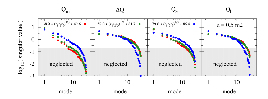
Note that here $\langle\ldots\rangle$ denotes the scalar product, i.e. the projection of $\Delta_{i}$ on ${\bf\hat{M}}_{i}$, while $\Delta_{i}$ is the same quantity which appears in equation (8). Fig. 20 shows that $\hat{C}_{ij}$ is typically dominated only by a few modes. Assuming that the modes with the lowest SVs can be associated with measurement noise, we use only SVs with values larger than the sampling error estimate (i.e. $\lambda^{2}\gtrsim\sqrt{2/N_{sim}}$) for our $\chi^{2}$ computation, as suggested by Gaztañaga & Scoccimarro (2005). The number of selected modes is hence the degree of freedom in our $\chi^{2}$ estimation, i.e. d.o.f. = $N_{mode}<N_{bin}<N_{sim}$.

3 accuracy of $Q$ predictions

The accuracy of bias measurements from the reduced three-point halo auto-correlation $Q_{h}$ in observations depends on how well it is approximated by the leading order perturbative model, given by equation (6). To verify this model we test its different components separately with direct measurements in the simulations described in Section 2.3. We start with testing the modeling of $Q_{m}$ in Section 3.1 and proceed in Section 3.2 with tests of the quadratic component in equation (6). Our measurements of the latter are obtained by combining the three-point auto- and cross-correlations, $Q_{h}$ and $Q_{\times}$ respectively. Finally, we compare the complete predictions for $Q_{h}$ and $Q_{\times}$, given by equation (6) and (7), with the measurements in the simulations in Section 3.3. For modeling the quadratic components we use bias parameters measured by CSS12 in the same set of simulations, using a leading order perturbative approximation of the 3PCF in Fourier space, i.e. the tree-level bispectrum. In addition we employ simple relations between the linear and the quadratic bias parameters, i.e. $b_{2}(b_{1})$ and $g_{2}(b_{1})$. This leaves $b_{1}$ as the only free input parameter in the bias model, which we adopt from the fits to the power spectrum, given by CSS12 (see Section 1.1).

Figure 1: Reduced matter 3PCF $Q_{m}$ for triangles with fixed legs $r_{1}$ and $r_{2}$ (size is indicated in $h^{-1}\text{Mpc}$) versus the mean triangle opening angle $\alpha\equiv\arccos(\hat{\bf r}_{1}\cdot\hat{\bf r}_{2})$ in each bin. Symbols show mean measurements from $49$ simulations with $1\sigma$ errors at redshift $z=0.5$. Lines show tree-level predictions from the measured (non-linear) power spectrum.

Figure 2: Significance of the deviations between the mean reduced matter 3PCF, measured in $49$ simulations and different tree-level predictions for the same triangle configurations as shown in Fig. 1. Dashed and solid lines show predictions from the linear and the measured (non-linear) power spectrum respectively. Predictions based on the de-wiggled power spectrum are shown as dashed-dotted lines. The black dotted lines mark $3\sigma$ deviations from the measurements.

3.1 $Q_{m}$

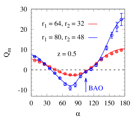
We start our verification of the $Q_{m}$ model from leading order (tree level) perturbation theory (hereafter referred to as $Q_{m}^{PT}$, see Section 2.2) by comparing its predictions to measurements in simulations. As examples we show in Fig. 1 results at redshift $z=0.5$ for triangles with fixed legs $(r_{1},r_{2})=(64,32)$ and $(80,48)$ $h^{-1}\text{Mpc}$ versus the triangle opening angle $\alpha\equiv\arccos(\hat{\bf r}_{1}\cdot\hat{\bf r}_{2})$. The $Q_{m}$ measurements are the mean results of the $49$ simulations and are shown with $1\sigma$ errors bars. Here and throughout the paper we display measurements at the mean opening angle in each bin. The predictions in Fig. 1 are computed from the non-linear power spectrum, which was measured in the simulations. Both, measurements and predictions exhibit a u-shape, which is more strongly pronounced for the larger triangle configuration and originates from the filamentary structure of the cosmic web. The measurements clearly show the baryon acoustic oscillations (BAO) feature for the $(80,48)$ $h^{-1}\text{Mpc}$ configuration at around $105^{\circ}$. Indications for similar BAO 3PCF features in real data have first been reported for luminous red galaxies in the SDSS DR7 sample by Gaztañaga et al. (2009). Slepian et al. (2015) later reported indications for the 3PCF BAO feature in the SDSS DR12 BOSS CMASS sample, which were comfirmed by the $4.5\sigma$ detection in the same data set by Slepian et al. (2017).

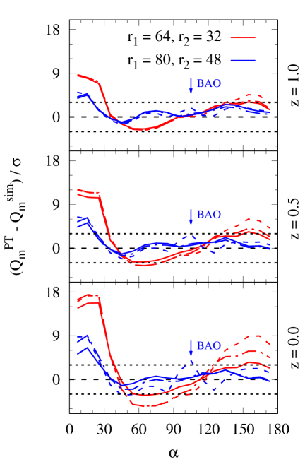
The significance of the deviations between measurements and predictions is shown for all redshifts in Fig. 2. In addition to the predictions from the non-linear power spectrum, we show in this figure also results based on the linear as well as the so-called de-wiggled power spectrum (hereafter also referred to as $P_{lin}$ and $P_{dw}$ respectively). The latter introduces non-linearities around the BAO scale in the 3PCF, coming from large-scale displacements (Crocce & Scoccimarro, 2008; Carlson et al., 2013; Baldauf et al., 2015; Senatore & Zaldarriaga, 2015; Blas et al., 2016). It consists of the no-wiggle approximation of the power spectrum ($P_{nw}$) from Eisenstein & Hu (1998), $P_{lin}$ and a smearing function, i.e., $P_{dw}\equiv P_{nw}+(P_{lin}-P_{nw})exp(-k^{2}\sigma_{v})$, where $k$ is the wave number and $\sigma_{v}$ is the variance of the displacement field (Eisenstein et al., 2007).

As a general trend we see in Fig. 2 that all predictions differ more significantly from the measurements for smaller triangles. This can be explained by the interplay of two effects. On one hand, terms in the perturbative expansion of $Q_{m}$ beyond leading order, which are neglected in our $Q_{m}$ model, contribute stronger at smaller scales. This explanation is consistent with the fact that the deviations are less significant at higher redshift and also when $Q_{m}^{PT}$ is computed from the non-linear, instead of the linear power spectrum. On the other hand, the signal-to-noise ratio is higher at small scales (see bottom panel of Fig. 15). Note that the latter is specific to the joint volume of our $49$ realisations of roughly $\sim 100\ (h^{-1}\text{Gpc})^{3}$. For the smaller volumes of current and near future galaxy surveys we expect the model to deviate less significantly because of larger measurement errors.

Predictions from the de-wiggled power spectrum are very similar to those from the linear power spectrum for smaller triangles (e.g. $(r_{1},r_{2})=(64,32)$ $h^{-1}\text{Mpc}$, $\alpha\lesssim 120^{\circ}$) and agree well with those from the non-linear power spectrum for large triangles (i.e. $(r_{1},r_{2})=(80,48)$ $h^{-1}\text{Mpc}$, $\alpha\gtrsim 90^{\circ}$). The latter finding indicates that for the tree-level calculation of the 3PCF in configurations space, implementing resummations over large-scale displacements by using the de-wiggled power spectrum has almost the same effect as using the non-linear spectrum from the simulation. For both cases the predictions are in $1\sigma$ agreement with the measurements at the BAO scale, while using the linear spectrum leads to $2-3\sigma$ deviations. For the remainder of our analysis we will use predictions based on the non-linear power spectrum, as they show the best overall agreement with the measurements in Fig. 2.

Figure 3: $Q_{m}$ measurements at $z=0.5$ versus the mean triangle opening angle per bin $\alpha$ and triangle scale $(r_{1}r_{2})^{1/2}$. Dots and solid contour lines show mean results from $49$ simulations. Dashed contour lines show tree-level predictions based on the non-linear power spectrum. The colours indicate the amplitude of $Q_{m}$.

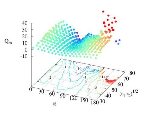
A convenient way to show results for all triangles in our analysis is to display them for a given opening angle $\alpha$ versus the triangle size, here defined as $\sqrt{r_{1}r_{2}}$. As an example we show the measurements of $Q_{m}$ in Fig. 3. This figure demonstrates the strong increase of the u-shape of $Q_{m}(\alpha)$ with the triangle scale. The minimum lies between $60$ and $90$ ^∘. Measurements for $\alpha\gtrsim 120$ ^∘and $\sqrt{r_{1}r_{2}}\gtrsim 50$ are dominated by noise.

Figure 4: Significance of the deviations between $Q_{m}$ measurements and tree-level predictions versus the mean triangle opening angle per bin $\alpha$ and the triangle scale $(r_{1}r_{2})^{1/2}$ in $h^{-1}\text{Mpc}$ at redshift $z=0.5$. The predictions are derived from the linear and measured (non-linear) power spectrum (top and bottom panel respectively). Black lines in the top panel trace the BAO feature $(r_{1}r_{2})^{1/2}(\alpha)$ for $r_{3}=95$$h^{-1}\text{Mpc}$. In the bottom panel black lines indicate the triangle scale at which the model fails at $2\sigma$, $(r_{1}r_{2}r_{3})^{1/3}\simeq 60$$h^{-1}\text{Mpc}$. In both cases solid and dashaed-dotted lines correspond to triangle configurations with of $r_{2}/r_{1}=1.0$ and $0.5$ respectively.

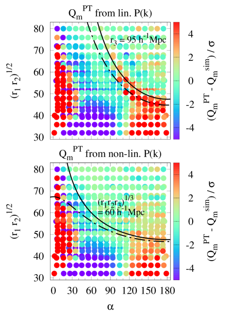
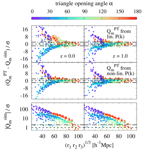
The significance of the deviations between $Q_{m}$ model predictions and measurements are shown for redshift $z=0.5$ versus $\alpha$ and $\sqrt{r_{1}r_{2}}$ in Fig. 4. We find that $Q_{m}^{PT}$ is below the measurements for opening angles between roughly $30-90$ ^∘for triangles with $30\lesssim\sqrt{r_{1}r_{2}}\lesssim 50$ $h^{-1}\text{Mpc}$. For smaller and larger opening angles the predictions tend to lie above the measurements. Similar results based on simulations with different cosmologies have been reported in the literature (see for instance Barriga & Gaztañaga (2002) or Hoffmann et al. (2015a), who use the same algorithms for the $Q_{m}$ predictions and measurements as employed in this study). Scoccimarro et al. (1998) showed that such deviations can be explained by higher order contributions as they reduce when the predictions are developed to next to leading order, including 1-loop terms (see also Sefusatti et al., 2010). As in Fig. 2 one can see in the top panel of Fig. 4 that using the linear power spectrum leads to strong deviations between predictions and measurements, in particular around the BAO peak, which are apparent as a red banana-shaped feature. This BAO feature follows roughly triangles with $r_{3}\sim 95$ $h^{-1}\text{Mpc}$, which are marked in the top panel as black lines. The deviations strongly reduce when the predictions are computed from the non-linear power spectrum for triangles scales $\sqrt{r_{1}r_{2}}\gtrsim 50$ $h^{-1}\text{Mpc}$ and $\alpha\gtrsim 30$ to roughly $1\sigma$.

Defining the overall triangle size as $(r_{1}r_{2}r_{3})^{1/3}$, we find that the deviations converge to $2\sigma$ at $(r_{1}r_{2}r_{3})^{1/3}\gtrsim 60$ ($80$) $h^{-1}\text{Mpc}$, when using the non-linear (linear) power spectrum (Fig. 15). Triangles with $(r_{1}r_{2}r_{3})^{1/3}=60$ $h^{-1}\text{Mpc}$ are therefore marked by black lines in the bottom panel of Fig. 4).

Figure 5: $\chi^{2}/d.o.f.$, quantifying the significance of the deviation between mean $Q_{m}$, measured in the simulations and tree-level predictions versus the mean triangle size $(r_{1}r_{2}r_{3})^{1/3}$ per bin. Lines and symbols show results for $Q_{m}$ predictions derived from the linear and non-linear power spectrum respectively at the redshifts $z=0.0$ and $z=0.5$.

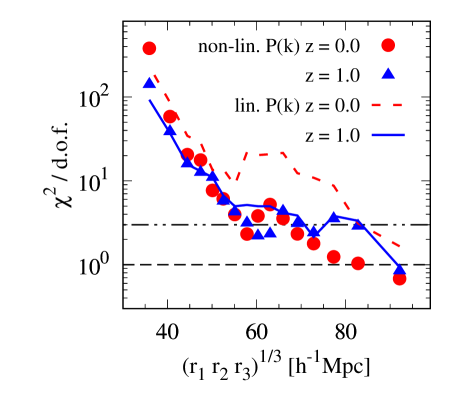
The normalised $Q_{m}$ covariance matrix, shown in Fig. 19, reveals that the $Q_{m}$ measurements for different triangles are correlated with each other. Hence, we compute an SVD estimate of the $\chi^{2}$ in bins of $(r_{1}r_{2}r_{3})^{1/3}$ to quantify the deviation between measurements and predictions, taking the covariance into account, as described in Section 2.4. Each $(r_{1}r_{2}r_{3})^{1/3}$ bin includes measurements from $30$ triangles, while we tested that our results change only weakly, when using $20$ and $40$ triangles per bin and do not affect our conclusions.

In Fig. 5, we find $\chi^{2}/d.o.f.$ values between $10$ and $100$ for $(r_{1}r_{2}r_{3})^{1/3}\lesssim 50$ $h^{-1}\text{Mpc}$ at $z=1.0$, where the degree of freedom ($d.o.f.$) is the number of singular values used for the $\chi^{2}$ estimation. At $z=0.0$ the $\chi^{2}/d.o.f.$ values are higher at small scales, indicating that $Q_{m}$ predictions agree better with measurements at higher redshifts. At $(r_{1}r_{2}r_{3})^{1/3}\gtrsim 60$ $h^{-1}\text{Mpc}$ the $\chi^{2}/d.o.f.$ values are roughly constant, taking values between $0.6-4$. An exception are the high values for the $Q_{m}$ model from the linear power spectrum at $z=0.0$, whereas using the non-linear and linear power spectra lead to similar results at $z=1.0$. These results indicated that non-linear contributions have a significant effect in $Q_{m}$ at small scales and low redshift and can partly be taken into account in the $Q_{m}$ predictions by using the non-linear power spectrum.

Note that the differences between results at different redshifts do not only result from different model performance, but also from differences in the covariances and modes selected for the $\chi^{2}$ computation. Since these quantities are sensitive to noise we will not enter a detailed discussion.

3.2 $\Delta Q$

In this subsection we test how well the higher-order contributions to the halo 3PCF are described by the quadratic $c_{2}+g_{2}Q_{nloc}$ term, which appears in equation (6) and (7). Following Bel et al. (2015), we obtain these higher-order contributions from the measurements by subtracting the halo-matter cross-correlation from the halo auto-correlation,

$$\Delta Q\equiv Q_{h}-Q_{\times}.$$ (12)

This subtraction leads to a cancellation of the linear $Q_{m}/b_{1}$ term in $Q_{h}$ and $Q_{\times}$ and hence isolates the higher-order terms. The aforementioned quadratic term correspond to the leading order perturbative approximation of $\Delta Q$, which follows from inserting the corresponding leading order approximations for $Q_{h}$ and $Q_{\times}$ from equation (6) and (7) into equation (12), i.e.

$$\Delta Q\simeq\frac{2}{3b_{1}}(c_{2}+g_{2}Q_{nloc}).$$ (13)

The relation above allows us to test on one hand the accuracy of the quadratic model for the higher order terms in $Q_{h}$ and $Q_{\times}$, independently of inaccuracies in the $Q_{m}$ modeling, which we studied previously in Section 3.1. On the other hand, we test simultaneously if the bias parameters, which we adopt from the Fourier space measurements of CSS12, also describe the clustering statistics in configurations space. Regarding the latter case we employ three sets of bias parameters to which we refer to as local, non-local and $b_{\delta^{2}fix}$ bias model, as described in Table 1, Section 1.1.

Figure 6: Top panels: $\Delta Q$ versus the mean triangle opening angle per bin $\alpha\equiv\arccos(\hat{\bf r}_{1}\cdot\hat{\bf r}_{2})$, measured at $z=0.5$ for the mass sample m2. Dashed and solid lines show tree-level predictions from the local and non-local bias model respectively, using the non-linear power spectrum and bias parameters measured in Fourier space by CSS12 in equation (13). Bottom panel: the significance of the deviation between model predictions and measurements.

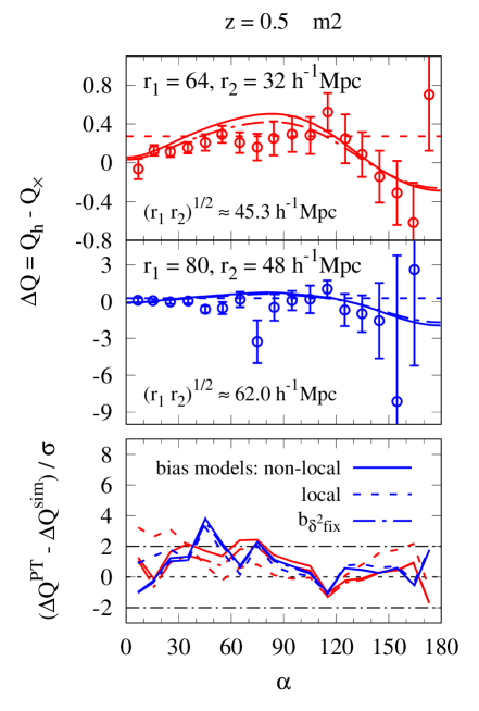
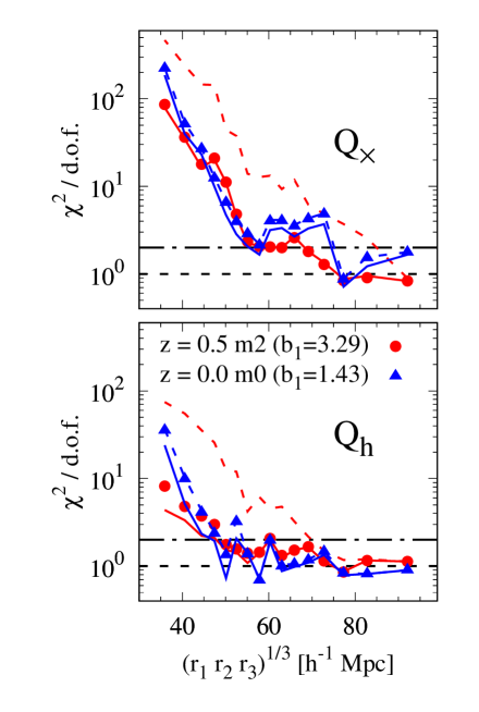
The corresponding model predictions for $\Delta Q$ are compared to the measurements at different triangle opening angles in Fig. 6. For this comparison we use the halo sample m2 at redshift $z=0.5$ (defined in Table 2) and the same triangle configurations as for the $Q_{m}$ in Fig. 1. The $\Delta Q$ measurements in Fig. 6 show a clear dependence on the triangle opening angle $\alpha$ for the small $(r_{1},r_{2})=(64,32)$ $h^{-1}\text{Mpc}$ triangle configuration. This finding contrasts the local bias model prediction of a constant $\Delta Q=2c_{2}/3b_{1}$. However, at intermediate angles ($60^{\circ}\lesssim\alpha\lesssim 120^{\circ}$) the local model predictions are in better agreement with the measurements than predictions from the non-local model. This result indicates that neglected higher order terms might compensate the quadratic non-local contribution.

Figure 7: Significance of the deviations between predictions for $\Delta Q$ and measurements for the mass samples m0 at $z=0.0$ and m2 at $z=0.5$ (top and bottom panels respectively). The results are shown versus the mean triangle opening angles per bin $\alpha$ and triangle scales $(r_{1}r_{2})^{1/2}$ in $h^{-1}\text{Mpc}$. The predictions are derived from the local, the non-local and the $b_{\delta^{2}fix}$bias model (see Table 1), with bias parameters measured in Fourier space by CSS12. Solid and dashed black lines in the bottom right panel show $(r_{1}r_{2})^{1/2}(\alpha)$ for $(r_{1}r_{2}r_{3})^{1/3}=60$$h^{-1}\text{Mpc}$ and triangle configurations of $r_{1}/r_{2}=0.5$ and $1.0$ respectively.

Similar trends are apparent for the larger ($80,48$) $h^{-1}\text{Mpc}$ triangle configuration, while here the large measurement errors lead to a similar significance of the different model deviations (see bottom panel of Fig. 6).

Note that for the presented results we computed $Q_{nloc}$ in equation (13) from the non-linear power spectrum, which was measured in the simulation. This is motivated by the fact that the $Q_{m}$ model performs better in that case (see Section 3.1). However, using $Q_{nloc}$ predictions from the linear power spectrum delivers very similar result and does not affect the conclusions drawn above.

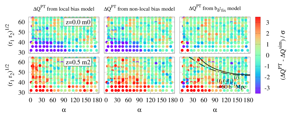
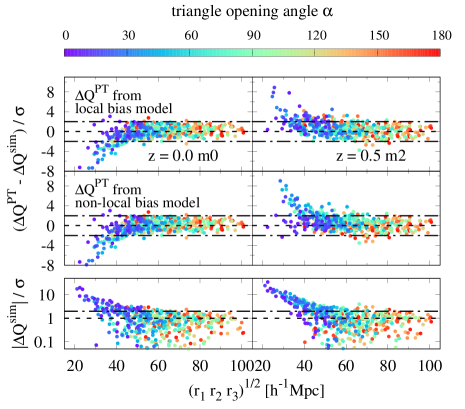
Extending the comparison between models and measurements to all triangles in our analysis, we show in Fig. 7 the significance of the deviations between $\Delta Q$ measurements and model predictions versus the triangle opening angle and scale $\sqrt{r_{1}r_{2}}$ (analogously to Fig. 4). We use again the mass sample m2 at $z=0.5$ (with $b_{1}=3.29$) and show in addition also results for the sample m0 at $z=0.0$ (with $b_{1}=1.43$) to explore how differences in the bias effect the model performance. For the highly biased sample m2 at $z=0.5$ (bottom panel of Fig. 7) the results line up with those for the two single triangle configurations, shown Fig. 6. For small triangles with $\sqrt{r_{1}r_{2}}\lesssim 40$$h^{-1}\text{Mpc}$ and triangle opening angles in the range of $60^{\circ}-120^{\circ}$ the local bias model is in better agreement with the measurements than the non-local model. Overall both models tend to overpredict the measurements at small triangle scales. The results for the $b_{\delta^{2}fix}$ model are very similar to those from the non-local model. This is also the case when the latter is based on the $b_{2}(b_{1})$ relation from Lazeyras et al. (2016).

These findings differ from those of the low biased sample m0 at $z=0.0$ (shown in top panel of Fig. 7) in three aspects. The first aspect is that the local and non-local model tend to underpredict the measurements for $\sqrt{r_{1}r_{2}}\lesssim 40$  $h^{-1}\text{Mpc}$. The second aspect is that for the low biased sample the local and non-local model perform equally well. This can be expected, since the non-local bias, measured by CSS12 is close to zero in that case. The third aspect is that the $b_{\delta^{2}fix}$ model differs from non-local model. In fact, it agrees better with the measurements than the other models. One interpretation of this result could be that the $c_{2}(b_{1})$ and $g_{2}(b_{1})$ relation is more accurate than the Fourier space measurements of the bias parameters from CSS12. Alternatively one might conclude that inaccuracies of the $b_{\delta^{2}fix}$ model compensate the neglected higher-order terms in the $\Delta Q$ model in equation (13), leading to a good agreement with the measurements by accident. To clarify this point one could repeat the exercise, using a model for $\Delta Q$ which is developed beyond second order. For a possible application of the $c_{2}(b_{1})$ and $g_{2}(b_{1})$ relations of the $b_{\delta^{2}fix}$ model in observations it would be interesting to test the dependence of our results on the cosmological parameters used. For bias measurements in observations it is also interesting to note that deviations between measurements in our $\sim 100\ (h^{-1}\text{Gpc})^{3}$ volume and model predictions become insignificant for $\sqrt{r_{1}r_{2}}\gtrsim 40$$h^{-1}\text{Mpc}$ as the measurement errors increase with scale.

As for $Q_{m}$ we find an overall convergence of the deviation between measurements and predictions for triangles with $(r_{1}r_{2}r_{3})^{1/3}$ $\gtrsim 60$ $h^{-1}\text{Mpc}$ in Fig. 16, which are marked in Fig. 7 with black lines.

Figure 8: $\chi^{2}/d.o.f.$, quantifying the significance of the deviation between the mean $\Delta Q$, measured in the simulations and predictions based on Fourier space bias parameters. Results are shown versus the mean triangle size $(r_{1}r_{2}r_{3})^{1/3}$ per bin. Dots are results based on the predictions from the non-local bias model. Results from the local and the $b_{\delta^{2}fix}$ bias model (see Table 1) are shown as dashed and solid lines respectively. Note that for the low biased mass sample m0 at redshift $z=0.0$ the results for the local and non-local bias are very similar since the non-local bias contribution is very small.

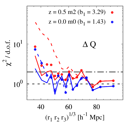
We quantify these deviations again by computing the $\chi^{2}$ via SVD, taking into account the covariance between measurements at different scales in $(r_{1}r_{2}r_{3})^{1/3}$ bins with $30$ triangles. Note that the $\Delta Q$ covariance is typically dominated by shot noise, coming from the $Q_{h}$ contribution, which can be seen in Fig. 19. The results, shown in Fig. 8 are in line with our finding from Fig. 16 as results converge to $\chi^{2}/d.o.f$ values around unity. The highly biased sample shows larger overall deviations between measurements and predictions, in particular for the non-local model at $(r_{1}r_{2}r_{3})^{1/3}$ $\lesssim 60$$h^{-1}\text{Mpc}$. Results for the $b_{\delta^{2}fix}$ model are similar to those from the non-local model at large scales, while at small scales the former performs better as its $\chi^{2}/d.o.f.$ values are lower.

Figure 9: Left: top panels show the reduced halo 3PCF, $Q_{h}$, for triangles with fixed legs $r_{1}$ and $r_{2}$ (size is indicated in $h^{-1}\text{Mpc}$) versus the mean triangle opening angle per bin, $\alpha\equiv\arccos(\hat{\bf r}_{1}\cdot\hat{\bf r}_{2})$. Symbols show mean measurements from $49$ simulations with $1\sigma$ errors for the mass sample m2 at redshift $z=0.5$. Lines show predictions from equation (6), using the non-linear power spectrum and the bias models from Table 1 with bias parameters measured by CSS12 in Fourier space. The bottom panel shows the significance of the deviations between model predictions and measurements. Right: analogous results for the reduced three-point halo-matter cross-correlations, while predictions are derived from equation (7).

3.3 $Q_{h}$ and $Q_{\times}$

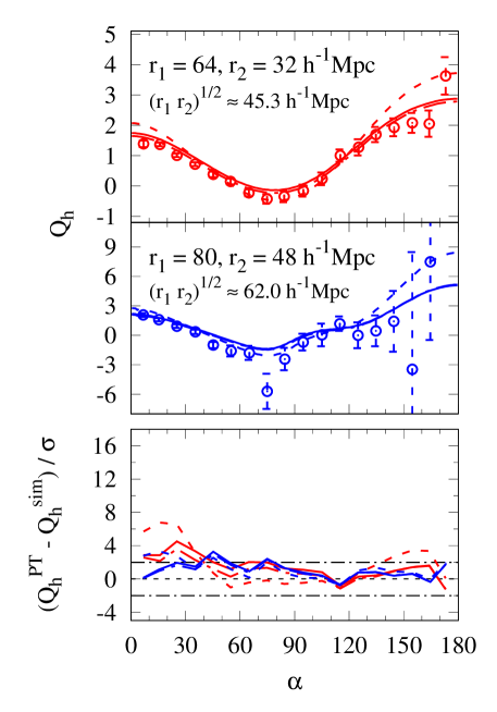
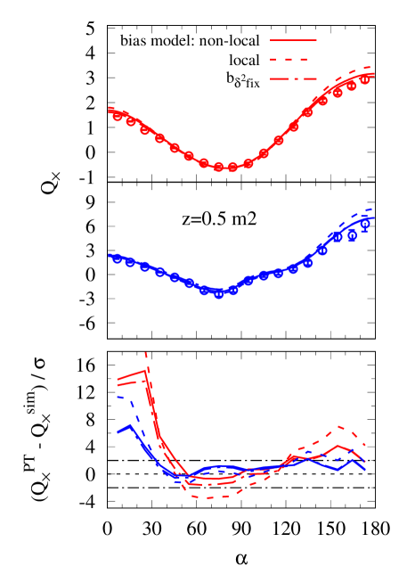
After validating the linear and quadratic components for the $Q_{h}$ and $Q_{\times}$ models separately in Section 3.1 and 3.2 we now compare the full models, given by equation (6) and (7) with the measurements in our simulations. As for $\Delta Q$ we focus on model predictions, which are based on the non-linear power spectrum and start the analysis by showing $Q_{h}$ and $Q_{\times}$, measured in the halo sample m2 at $z=0.5$, for triangles with fixed legs of $(r_{1},r_{2})=(64,32)$ and $(80,48)$$h^{-1}\text{Mpc}$ versus the triangle opening angle $\alpha$ in Fig. 9. We find that the models for both, $Q_{h}$ and $Q_{\times}$ tend to overpredict the measurements, which lines up with our corresponding results for $\Delta Q$ in Fig. 6. An exception of this trend are $Q_{h}$ results from the small triangle configuration with $60\lesssim\alpha\lesssim 90$. This indicates that the neglected terms in the perturbative model beyond leading order affect $Q_{h}$ and $Q_{\times}$ differently. Again, the model predictions based on the local bias model show the strongest deviations from the measurements, in particular for collapsed and relaxed triangles. This explains why neglecting the non-local term leads to an overestimation of the bias, when fitting $Q_{h}$ or $Q_{\times}$ model predictions to measurements (see CSS12). For such a fit one would choose a higher $b_{1}$, since this would flatten the curve and deliver the measured shape. The overall amplitude can then be adjusted by varying $c_{2}$ (see equation (6)). Such fits of the local model are in fact in very good agreement with the measurements. However, the linear bias is too high (e.g. Manera & Gaztañaga, 2011; Bel et al., 2015). Note that the linear bias measurements based on the local bias model would be too low instead of too high when using the 3PCF or the bispectrum, as explained by CSS12.

The best agreement between the $Q_{h}$ and $Q_{\times}$ measurements and the corresponding models occurs at large opening angles (hence large triangles) when using the non-local bias model ($1-2\sigma$). This scale dependence can be expected since errors increase and higher order contributions decrease with the scale. Results based on the $b_{\delta^{2}fix}$ model are again very similar to those from the non-local model.

Interestingly the deviations between the model predictions and measurements are less significant for $Q_{h}$ than for $Q_{\times}$, despite the fact that the neglected terms beyond leading order should have a higher contribution to $Q_{h}$ and therefore lead to stronger deviations from the model. However, the errors on $Q_{h}$ are more strongly affected by shot-noise than those for $Q_{\times}$ ($\sigma^{2}_{Q_{h}}\sim n_{h}^{3}$, $\sigma^{2}_{Q_{\times}}\sim n_{h}$, where $n_{h}$ is the halo number density). This means that for observations with similar or larger errors than our measurements, a development of the $Q_{h}$ model beyond leading order might only lead to a marginal improvement of the model performance.

Figure 10: Significance of the deviations between predictions for $Q_{\times}$ and $Q_{h}$ and measurements for the mass samples m0 at $z=0.0$ and m2 at $z=0.5$ (top, bottom panels respectively). The results are shown versus the mean triangle opening angles per bin, $\alpha$, and triangle scales $(r_{1}r_{2})^{1/2}$ in $h^{-1}\text{Mpc}$. The predictions are derived from the bias models described in Table 1, with bias parameters measured in Fourier space by CSS12. Solid and dashed black lines in the bottom right panel show $(r_{1}r_{2})^{1/2}(\alpha)$ for $(r_{1}r_{2}r_{3})^{1/3}=60$$h^{-1}\text{Mpc}$ and triangle configurations of $r_{1}/r_{2}=0.5$ and $1.0$ respectively.

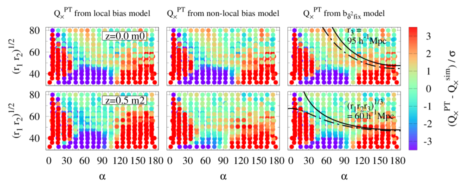
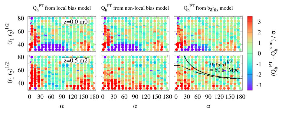
In Fig. 10 we show the comparison between $Q_{\times}$ and $Q_{h}$ models and measurements for all triangles, displaying them for different scales $\sqrt{r_{1}r_{2}}$ versus the triangle opening angle (as in Fig. 7). Results are shown for the low biased sample m0 at $z=0.0$ and the highly biased sample m2 at $z=0.5$. The latter confirm the trends from from Fig. 9. In particular for small triangles ($\sqrt{r_{1}r_{2}}\lesssim 40$$h^{-1}\text{Mpc}$) the $Q_{\times}$ and $Q_{h}$ models overpredict the measurements for collapsed and relaxed triangles and underpredict them for triangles with $60\lesssim\alpha\lesssim 90$. The $Q_{h}$ results for m2 at $z=0.5$ are again an exception. In that case the local model is in better agreement with the measurements than the non-local model, which is consistent with the $\Delta Q$ results for this sample and might be attributed to a compensation of quadratic non-local and neglected higher-order terms, as mentioned in the discussion of Fig. 6 in Section 3.2. Note that this compensation is shown here to occur for one particular halo sample, while this is not the case for other samples (not shown here).

Overall the results from the non-local bias model are in better agreement with the measurements for the sample m2 at $z=0.5$ than the local model at large triangles scales ($\sqrt{r_{1}r_{2}}\gtrsim 40$ $h^{-1}\text{Mpc}$ or $\alpha\gtrsim 90$) and are consistent with those from the $b_{\delta^{2}fix}$ model. For the low biased sample m0 at $z=0.0$ all bias models deliver similar results, since the non-local bias contribution is very weak. For some triangles we find an increased significance of the deviations for that sample, compared to the m2 sample at $z=0.5$, presumably because the shot noise error contribution is decreased due to the higher halo density. In the case of $Q_{\times}$, where the shot noise errors are the lowest, the deviations follow the BAO feature, which we saw already in the $Q_{m}$ model validation (Fig. 7). Using model predictions based on the linear power spectrum, we find a significant increase of the deviations in the case of $Q_{\times}$ for both samples (not shown here). This indicates that neglected terms in the $Q_{m}$ model, in the bias model or both affect the halo 3PCF, even at very large triangle scales. However, for the auto-correlation $Q_{h}$ at $\sqrt{r_{1}r_{2}}\gtrsim 40$ $h^{-1}\text{Mpc}$ their contribution seems to be small compared to the measurement errors, as we find a similarly significant deviations for different power spectra and halo samples. This will in particular be also the case for the smaller volumes, covered by galaxy surveys, for which the measurement errors can be expected to be larger.

The deviations between non-local bias model predictions and measurements converge to values of $\lesssim 2\sigma$ $(r_{1}r_{2}r_{3})^{1/3}$$\gtrsim 60$$h^{-1}\text{Mpc}$ (marked in Fig. 10 as black lines) for both, $Q_{\times}$ and $Q_{h}$, as shown in Fig. 17 and 18. This is consistent with our corresponding results for $Q_{m}$ and $\Delta Q$.

Figure 11: Top: $\chi^{2}$ per degree of freedom (d.o.f.), quantifying the difference between the $Q_{\times}$ measurements for the mass samples m1, m2, m3 (defined in Table 2) and the corresponding predictions, based on the non-linear power spectrum at different redshifts $z$. Symbols show results for the non-local bias model, while lines show results using analytical relations between the linear and non-linear bias parameters ($b_{\delta^{2}fix}$ model, see Table 1). The bias parameters were measured by CSS12 in Fourier space. Bottom: same as top panel, but for $Q_{h}$.

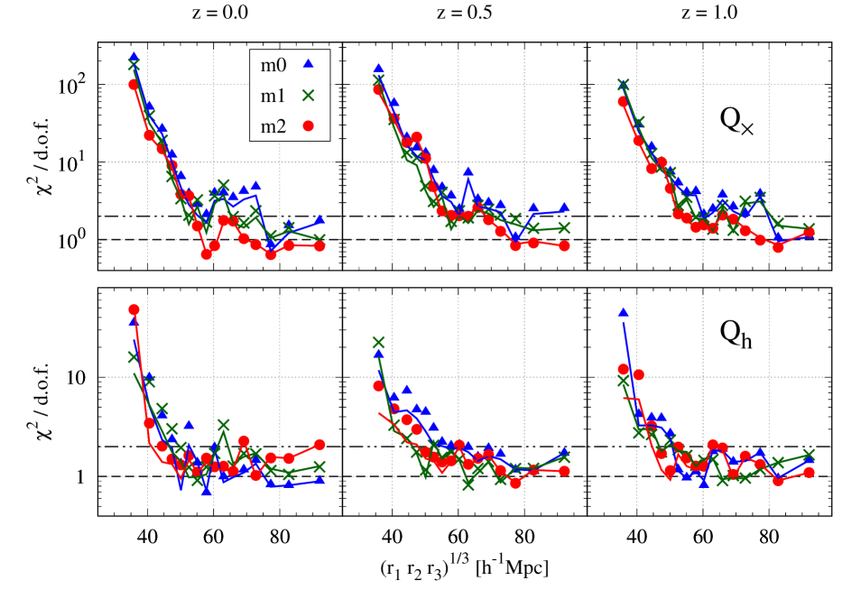
As in the case of $Q_{m}$ and $\Delta Q$, measurements of $Q_{h}$ and $Q_{\times}$ from different triangles are covariant (see Fig. 19). Quantifying the significance of deviations between model predictions and measurements, we show in Fig. 11 the $\chi^{2}/d.o.f.$ in bins of $(r_{1}r_{2}r_{3})^{1/3}$ for all three mass samples and redshifts. Each bin contains measurements from $30$ triangles and the $\chi^{2}$ values have been computed via SVD (see Section 2.4) using only the dominant modes, as for the $Q_{m}$ and $\Delta Q$ analyses from Fig. 5 and 8. We also tested that our results are not affected by the chosen number of triangles per bin. The results confirm the convergence of the deviations to $1-2\sigma$ for $(r_{1}r_{2}r_{3})^{1/3}$ $\gtrsim 60$ $h^{-1}\text{Mpc}$. However, they show strong variations for different scales, which might result from noise in our covariance estimation from only $49$ realisations. Overall, the $\chi^{2}/d.o.f.$ values for $Q_{\times}$ are higher than those for $Q_{h}$, presumably because of the higher signal-to-noise ratio of the measurements. Even at large scales above $60$ $h^{-1}\text{Mpc}$ we find $\chi^{2}/d.o.f.\simeq 5$ values. They might be explained by non-linearities around the BAO feature, which are not fully captured in our leading order perturbative model (see Fig. 10). For $Q_{\times}$ the $\chi^{2}/d.o.f.$ values are lower at high redshift and higher mass samples. The latter result might be explained by larger shot-noise errors on the high mass samples and agrees with the results from Fig. 17 and 18. Smaller deviations at high redshifts might result from a smaller impact of next to leading order terms in the $Q_{\times}$ model, which we neglect in our analysis. We do not see a clear dependence of the results on mass and redshift for $Q_{h}$, possibly because of the low signal-to noise ratio. It is interesting to note that the $\chi^{2}/d.o.f.$ values for the $b_{\delta^{2}fix}$ model are in very good agreement with those from the non-local model for highly biased sample (high halo mass and redshift). For samples with low bias (low mass, low redshift) the $\chi^{2}/d.o.f.$ values for the $b_{\delta^{2}fix}$ are even smaller than those for the non-local model. The latter finding is consistent with our model comparison for $\Delta Q$.

Our comparison between $\chi^{2}/d.o.f.$ values for local and non-local model predictions in Fig. 12 demonstrates that setting the non-local term in the prediction to zero leads to higher deviations from $Q_{\times}$ measurements for highly biased samples. The effect is also apparent for $Q_{h}$, even for $(r_{1}r_{2}r_{3})^{1/3}$ $>60$ $h^{-1}\text{Mpc}$, while in that case the $\chi^{2}/d.o.f.$ values are lower, presumably due to larger errors on the measurements. Again these results confirm those for $\Delta Q$, shown in Fig. 8.

Figure 12: The figure shows the same results for the non-local and $b_{\delta^{2}fix}$ model as shown in Fig. 11 for the mass sample m0 at $z=0.0$ m2 at $z=0.5$. In addition we show here results for the local model as dashed lines.

4 Summary and Conclusions

The main result of this paper (summarized in Fig. 11) is an empirical determination of the scales at which three-point halo correlations in configuration space are consistent with the corresponding statistics in Fourier space, i.e. the bispectrum. To this end, we measured the reduced three-point auto-correlation function of matter and halos, as well as the reduced halo-matter three-point cross-correlation (which are referred to as $Q_{m}$, $Q_{h}$ and $Q_{\times}$ respectively) in a set of $49$ cosmological simulations with a total volume of $\sim 100\ (h^{-1}\text{Gpc})^{3}$. The large volume provides small errors on the measurements. At the same time we obtain rough estimates of the error covariances, which we analysed using singular value decomposition. The $Q_{h}$ and $Q_{\times}$ measurements were compared to leading order perturbative models (equation (6) and (7)), which relate these statistics to $Q_{m}$ via the linear, quadratic and non-local bias parameters (referred to as $b_{1}$, $c_{2}$ and $g_{2}$ respectively). For testing the consistency with results from Fourier space, we adopted bias parameters, which were measured in the same set of simulations by Chan et al. (2012, referred to as CSS12) using the same perturbative model of the halo-matter cross-bispectrum.

We adopted the bias parameters in three different ways. The first way is to simply employ the set of Fourier space parameter from CSS12. The second set of parameters are identical to the first set, except for the non-local bias parameter $g_{2}$, which is set to zero in order to study the contribution of the non-local terms to the $Q_{h}$ and $Q_{\times}$ predictions. For the third set we used the linear bias, measured by CSS12 from the halo-matter cross-power spectrum, while the quadratic bias is set by the (approximately) universal $c_{2}(b_{1})$ relation from Hoffmann et al. (2017) and the non-local bias is predicted using the $g_{2}(b_{1})$ relation from the local Lagrangian model, reducing the degrees of freedom in the bias model. These three sets of bias parameters are referred to as non-local, local and $b_{\delta^{2}fix}$ model respectively and are summarized in Table 1.

Before predicting $Q_{h}$ and $Q_{\times}$ using the bias parameters, we first had to obtain the matter contribution $Q_{m}$ and the non-local contribution $Q_{nloc}$. To remain closer to an analysis of observational data, where these quantities cannot be directly measured, we modeled them from the linear, the linear de-wiggled and the non-linear power spectrum. By comparing the $Q_{h}$ and $Q_{\times}$ predictions to measurements, we therefore did not only test if the bias parameters in Fourier space describe the clustering in configurations space, but also simultaneously at which scales the perturbative model of the three-point correlation breaks down. We conducted this comparison in three steps. We first studied in Section 3.1 how well $Q_{m}$ measurements are described by the leading order perturbative predictions from the different power spectra. Secondly, we investigate how well the higher-order contributions to $Q_{h}$ are described by the leading (quadratic) order perturbative models, based on the Fourier space bias parameters. These contributions are obtained from the measurements by the subtraction $\Delta Q\equiv Q_{h}-Q_{\times}$, as described in Section 3.2. Finally, we compare in Section 3.3 the full predictions for for $Q_{h}$ and $Q_{\times}$ with the corresponding measurements.

Overall our results show that the deviations between the model predictions for $Q_{m}$, $Q_{h}$, $Q_{\times}$ and $\Delta Q$ and the corresponding measurements depends on the triangle scale as well as on the triangle shape (characterised by the triangle opening angle) for which these statistics are studied. The quantity $(r_{1}r_{2}r_{3})^{1/3}$ turns out to be a convenient definition of the triangle scale, since it shows a tight correlation with the measurement errors. Furthermore it separates well larger triangles for which the models perform well from smaller ones, for which the measurements are presumably strongly affected by higher order terms. We found that the deviation between the perturbative model predictions of the different three-point correlations from the measurements converge to the $1-2\sigma$ level for $(r_{1}r_{2}r_{3})^{1/3}\gtrsim 60$ $h^{-1}\text{Mpc}$, while the noisy error estimation imposes some uncertainty on this value. Note here that the smallest $r_{i}$ value above zero in our analysis corresponds to the size of the $8$ $h^{-1}\text{Mpc}$ grid cells into which we divided the simulations for computing the correlations. However, when the measurement errors are small (in particular their shot-noise contribution), which is the case for $Q_{m}$ and $Q_{\times}$, and when the predictions are computed from the linear instead of the non-linear power spectrum, we find deviations above $2\sigma$ for $(r_{1}r_{2}r_{3})^{1/3}\gtrsim 60$$h^{-1}\text{Mpc}$. We attribute this effect to non-linearities around the BAO peak from large scale displacements and bias contributions not included in our treatment. The fact that this effect is much weaker when using the de-wiggled, or the non-linear power spectrum indicates that the latter can incorporate higher orders in the perturbative model for $Q$ to some degree.

Validating the model for the quadratic terms in $Q_{h}$ and $Q_{\times}$ with the $\Delta Q$ measurements, we found the predictions based on the non-local bias model to show an overall better performance than those from the local model. An exception are measurements in highly biased halo samples from small triangles with intermediate opening angles, which are better described by the local than the non-local bias model. We interpret this effect as a compensation of the non-local and the higher order terms not included in our bias treatment, which occurs for these particular triangles and this particular halo sample.

Interestingly, the deviations of the $\Delta Q$ predictions based on the $b_{\delta^{2}fix}$ bias model from the measurements are similar, and for low biased samples even smaller than those based on the non-local model. For $(r_{1}r_{2}r_{3})^{1/3}\gtrsim 60$$h^{-1}\text{Mpc}$ the significance of the deviations between $\Delta Q$ predictions and measurement is similar for all bias models, presumably because of the low signal-to-noise ratio.

From the $Q_{\times}$ measurements we conclude that the leading order perturbative model predictions in combination with the bias derived from the same statistics in Fourier space are a good approximation, with $1-2\sigma$ deviations $(r_{1}r_{2}r_{3})^{1/3}\gtrsim 60$$h^{-1}\text{Mpc}$. These deviation are slightly higher around the aforementioned BAO feature, but given the small errors on $Q_{\times}$ this agreement is still good. The model performance for $Q_{h}$ at large scales is even better, despite the fact that terms beyond leading order, which are neglected in the model should affect $Q_{h}$ more strongly than $Q_{\times}$. This might be a result of the lower signal-to-noise ratio. However, the $Q_{h}$ predictions differ significantly from the measurements for $(r_{1}r_{2}r_{3})^{1/3}\lesssim 50$$h^{-1}\text{Mpc}$. It is thereby important to note, that these results are specific to our small measurement errors from the combined $\sim 100\ (h^{-1}\text{Gpc})^{3}$ of the $49$ simulations studied in this work. In practice, the deviation between model predictions and measurements can be expected to be less significant, as the measurement errors are larger for the smaller volumes of current and upcoming galaxy surveys.

As for $\Delta Q$, the $Q_{h}$ and $Q_{\times}$ predictions from the $b_{\delta^{2}fix}$ model agree equally well with the measurements at large scales for highly biased samples (high masses, high redshift). For low biased samples (low mass, low redshift) this model describes the $Q_{h}$ and $Q_{\times}$ measurements even better than the non-local model. Differences in the $Q_{h}$ predictions based on the linear and non-linear power spectrum are negligible compared to the larger measurement errors.

The good performance of predictions from the $b_{\delta^{2}fix}$ model at larges scales suggests that a roughly universal $c_{2}(b_{1})$ relation, together with the local Lagrangian $g_{2}(b_{1})$ relation, could tighten constraints on the linear bias, derived from third-order statistics in galaxy surveys. However, recent studies pointed out, that assembly bias can lead to deviations from a universal $c_{2}(b_{1})$ relation (Modi et al., 2016; Paranjape & Padmanabhan, 2017). An application of the $b_{\delta^{2}fix}$ model in the analysis of galaxy surveys therefore requires tests in mock catalogues (for instance from semi-analytic models of galaxy formation) to validate for which type of galaxy samples these bias relations are useful approximations. More generally, the results presented in this paper show a good overall agreement of the non-local quadratic bias models with simulations, using the same bias parameters for Fourier and configuration space, but the range of validity will depend strongly on the samples used (volume, redshift and bias), so a detailed comparison with mock galaxy and corresponding dark matter catalogues with redshift space distortions will be needed.

Appendix A 3PCF binning

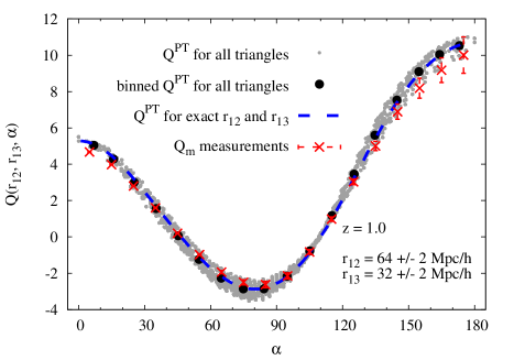
When measuring the 3PCF on a grid of cubical cells, we need to allow for a tollerance of the triangle leg sizes $(r_{12},r_{13})$ to obtain a sufficiently larger number of triangles in each bin of the triangle opening angle $\alpha$ (see Section 2.3). Here we test for different triangle configurations how much the results are affected by this tolerance. We therefore compute the matter 3PCF prediction for all triangles on the grid, which fulfill the condition $(r_{12},r_{13})\pm(\delta r_{12},\delta r_{13})$. As an example we show the results for the configuration $(64,32)\pm(2,2)$ $h^{-1}\text{Mpc}$ in Fig. 13 as grey dots versus $\alpha$. The average 3PCF predictions in bins of $\alpha$ are shown as black dots at the mean angle in each bin. These results are compared to predictions for exact values of $(r_{12},r_{13})$ (i.e. $(\delta r_{12},\delta r_{13})=(0,0)$). We find that the difference between the two types of predictions is small, compared to the difference between predictions and measurements (red symbols). We obtain the same results for different triangle configurations (not shown here) and conclude that the binning of the 3PCF measurements has no significant impact on the compariosn with the unbinned theory predictions, which we use in our analysis.

Figure 13: Testing the impact of the grid on the 3PCF. Grey dots show the predictions for the matter 3PCF, based on the measured power spectrum at $z=1.0$, for all triangles with $(r_{12},r_{13})\pm(\delta r_{12},\delta r_{13})=(64,32)\pm(2,2)$ $h^{-1}\text{Mpc}$ on the grid versus the opening angles $\alpha$. The mean predictions in bins of $\alpha$ are shown as black dots. Predictions for $(\delta r_{12},\delta r_{13})=(0,0)$ (as we use them in our analysis) are shown as dashed blue line. Measurements of the 3PCF at $z=0.0$ are shown with $1\sigma$ errors as red symbols.

Appendix B Deviations for individual triangles

Figure 14: Examples of $1\sigma$ errors of the different reduced 3PCFs studied in this paper versus the triangle scale. Results for different redshifts and mass samples are similar.

The errors of the different $Q$ measurements correlates strongly with the total triangle scale, defined by $(r_{1}r_{2}r_{3})^{1/3}$ as shown in Fig. 14. We therefore study here the significance of the deviations between measurements and predictions versus this scale.

Fig. 15 shows that the $Q_{m}$ predictions deviate from the measurements by less than $2\sigma$ for $(r_{1}r_{2}r_{3})^{1/3}\gtrsim 80$ when predictions are computed from the linear power spectrum and $\gtrsim 60$ $h^{-1}\text{Mpc}$ when using the non-linear power spectrum. Note that these results are specific for the joint $\sim 100\ (\text{Gpc}/h)^{3}$ volume of the $49$ simulations. For smaller volumes (as covered by current galaxy surveys) errors would be larger and the significance therefore smaller. Using alternative measures for the triangle scale, such as the triangle area or the sum of the triangle legs leads to a less clear separation between triangles with weak and strong significance of the deviations.

Figure 15: Top panels: Significance of the deviation between $Q_{m}$ measurements and tree-level predictions (based on the linear and non-linear power spectrum) versus the triangle scale. Dashed- dotted lines denote $2\sigma$ deviations. Bottom panel: Signal-to-noise ratio. Colours denote the triangle opening angle.

The corresponding results for $\Delta Q$ are shown in Fig. 16 for the low biased sample (m0) at $z=0.0$ and the highly biased sample (m2) at $z=0.5$ (with $b_{1}=1.43$ and $b_{1}=3.29$ respectively). For the sample with the low linear bias the model predictions are below the measurements at $(r_{1}r_{2}r_{3})^{1/3}$ $\lesssim 60$ $h^{-1}\text{Mpc}$. Differences between local and non-local model predictions are not apparent, as expected from Fig. 7. For the sample with the higher linear bias the predictions are above the measurements for $(r_{1}r_{2}r_{3})^{1/3}$ $\gtrsim 60$ $h^{-1}\text{Mpc}$ and the non-local model performs slightly better than the local model at small scales. At large scales differences between model and predictions are not signifiant for both samples, due to the low signal-to-noise ratio, which is shown in the bottom panel of Fig. 16. Note that the predictions are based on the non-linear power spectrum, measured in the simulation, while the linear power spectrum leads to very similar results.

Figure 16: Significance of the deviation between predictions for $\Delta Q$ and measurements versus triangle scale $(r_{1}r_{2}r_{3})^{1/3}$ for the halo mass samples m0 at $z=0.0$ and and m1 at $z=0.5$ (left and right panels respectively). The top and central panels show results for predictions from the local and non-local model respectively (Table 1), based on the non-linear power spectrum. The bottom panel shows signal-to-noise ratio of measurements.

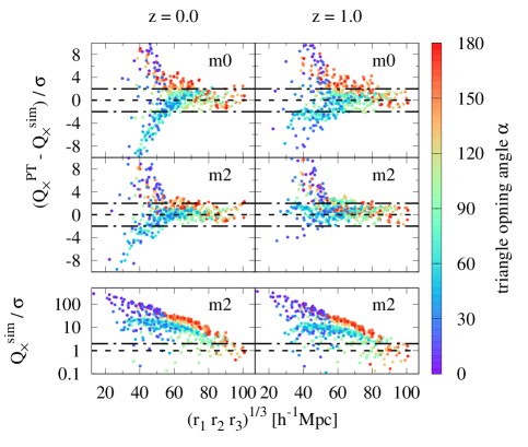
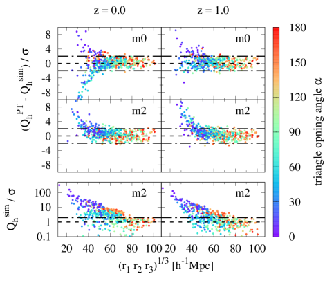
The significance of the deviations between non-local bias model predictions for $Q_{h}$ and $Q_{\times}$ and the corresponding measurements are displayed versus the triangle scale in Fig. 17 and 18. Covering a larger range of bias values ($1.43\lesssim b_{1}\lesssim 3.99$), we now show results for the mass samples m0 and m2, each at redshift $z=0.0$ and $1.0$. Also here the predictions are based on the non-linear power spectrum and we find very similar results when using the linear power spectrum. The results are consistent with those shown in Fig. 10 as the predictions are most significant for small triangles, where they show a strong dependence on the triangle opening angle for low biased samples, while samples with high bias (higher masses and redshifts) show a weaker dependence on the opening angle at small scales. Overall the deviations for both, $Q_{\times}$ and $Q_{h}$ converge to values of $\lesssim 2\sigma$ for all samples for $(r_{1}r_{2}r_{3})^{1/3}$$\gtrsim 60$$h^{-1}\text{Mpc}$. An exception are results $Q_{\times}$ for large opening angles, which can be attributed non-linearities around the BAO peak, as mentioned in the discussion of Fig. 10.

Figure 17: Significance of the deviations between predictions for $Q_{\times}$ and measurements versus triangle scale $(r_{1}r_{2}r_{3})^{1/3}$. The predictions are based on the non-local bias model (Table 1) and the non-linear power spectrum. Results are shown for the halo mass samples m0 and m2 at $z=0.0$ and $z=1.0$ (left and right, top, bottom panels respectively). The lower sub panels show the signal-to-noise ratios for the samples m2, which have higher shot-noise contributions than the m0 sample.

Figure 18: same as Fig. 17, but for $Q_{h}$.

Appendix C Covariances

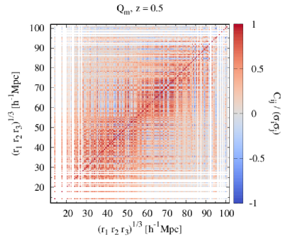
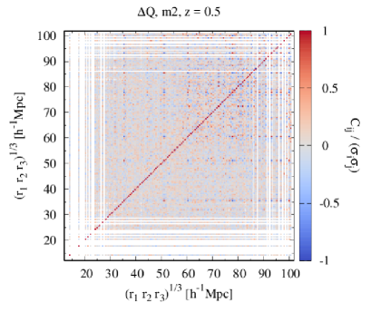
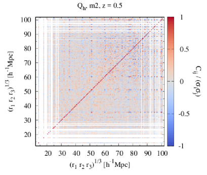
In Fig. 19 we show examples of the normalised covariance matrices at $z=0.5$ for the different three-point statistics versus the triangle scale $(r_{1}r_{2}r_{3})^{1/3}$. The covariances for $Q_{m}$ and $Q_{\times}$ show strong off-diagonal elements, while those of $Q_{h}$ and $\Delta Q$ are dominated by the diagonal elements, which indicates high shot-noise contributions. Subsets of these covariances with $30^{2}$ elements around the diagonal are used for the $\chi^{2}$ estimation, described in Section 2.4.

In order to reduce the impact of noise on these estimations we perform a singular value decomposition of the covariances. The distribution of singular values is shown in Fig. 20 and reveals that a significant fraction of modes has only a minor contribution to the covariance. One can see how the singular values for the shot-noise dominated covariances of $\Delta Q$ and $Q_{h}$ show a slightly more pronounced drop, while those of the $Q_{m}$ and $Q_{\times}$ covariances decay more slowly. We associate modes below $\lambda^{2}\lesssim\sqrt{2/N_{sim}}$ with noise in the covariance measurement and neglect them in the $\chi^{2}$ computation.

Figure 19: Examples of normalised covariances between different reduced 3PCS from the $504$ triangles used in this work. They were obtained from a set of $49$ simulations. The low amplitude of the off-diagonal elements in the $Q_{h}$ covariances indicates a dominance of shot-noise errors. Results for $Q_{h}$ and $Q_{\times}$ are almost identical, because the $Q_{\times}$ errors are dominated by the $Q_{h}$ contribution. For computing the $\chi^{2}$ deviation from the model prediction we select triangles in scale bins containing $30$ triangles and perform a singular value decomposition, as described in Section 2.3.

Figure 20: Singular values of the covariance matrices for the different three-point statistics studied in this work versus the mode number. The maximum mode number corresponds to the number of triangles in the $(r_{1}r_{2}r_{3})^{1/3}$ bins. Results are shown for the mass sample m1 at $z=0.5$. Modes with singular values of less than $\lambda^{2}\lesssim\sqrt{2/N_{sim}}$ are associated with noise and therefore neglected in the $\chi^{2}$ computation. The total number of modes is $30$, which corresponds to the number of triangles in each $(r_{1}r_{2}r_{3})^{1/3}$ bin.

References

- Baldauf et al. (2012) Baldauf T., Seljak U., Desjacques V., McDonald P., 2012, Phys. Rev. D, 86, 083540
- Baldauf et al. (2015) Baldauf T., Mirbabayi M., Simonović M., Zaldarriaga M., 2015, Phys. Rev. D, 92, 043514
- Barriga & Gaztañaga (2002) Barriga J., Gaztañaga E., 2002, MNRAS, 333, 443
- Bel et al. (2015) Bel J., Hoffmann K., Gaztañaga E., 2015, MNRAS, 453, 259
- Berlind & Weinberg (2002) Berlind A. A., Weinberg D. H., 2002, ApJ, 575, 587
- Blas et al. (2016) Blas D., Garny M., Ivanov M. M., Sibiryakov S., 2016, J. Cosmology Astropart. Phys., 7, 028
- Byun et al. (2017) Byun J., Eggemeier A., Regan D., Seery D., Smith R. E., 2017, MNRAS, 471, 1581
- Carlson et al. (2013) Carlson J., Reid B., White M., 2013, MNRAS, 429, 1674
- Chan & Blot (2016) Chan K. C., Blot L., 2016, preprint, (arXiv:1610.06585)
- Chan et al. (2012) Chan K. C., Scoccimarro R., Sheth R. K., 2012, Phys. Rev. D, 85, 083509
- Cooray & Sheth (2002) Cooray A., Sheth R., 2002, Phys. Rep., 372, 1
- Crocce & Scoccimarro (2008) Crocce M., Scoccimarro R., 2008, Phys. Rev. D, 77, 023533
- Desjacques et al. (2016) Desjacques V., Jeong D., Schmidt F., 2016, preprint, (arXiv:1611.09787)
- Eisenstein & Hu (1998) Eisenstein D. J., Hu W., 1998, ApJ, 496, 605
- Eisenstein et al. (2007) Eisenstein D. J., Seo H.-J., White M., 2007, ApJ, 664, 660
- Frieman & Gaztanaga (1994) Frieman J. A., Gaztanaga E., 1994, ApJ, 425, 392
- Fry (1984) Fry J. N., 1984, ApJ, 279, 499
- Fry & Gaztanaga (1993) Fry J. N., Gaztanaga E., 1993, ApJ, 413, 447
- Gaztañaga & Scoccimarro (2005) Gaztañaga E., Scoccimarro R., 2005, MNRAS, 361, 824
- Gaztañaga et al. (2009) Gaztañaga E., Cabré A., Castander F., Crocce M., Fosalba P., 2009, MNRAS, 399, 801
- Gaztanaga & Bernardeau (1998) Gaztanaga E., Bernardeau F., 1998, A&A, 331, 829
- Gil-Marín et al. (2015) Gil-Marín H., Noreña J., Verde L., Percival W. J., Wagner C., Manera M., Schneider D. P., 2015, MNRAS, 451, 539
- Gualdi et al. (2017) Gualdi D., Manera M., Joachimi B., Lahav O., 2017, preprint, (arXiv:1709.03600)
- Hartlap et al. (2007) Hartlap J., Simon P., Schneider P., 2007, A&A, 464, 399
- Hoffmann et al. (2015a) Hoffmann K., Bel J., Gaztañaga E., Crocce M., Fosalba P., Castander F. J., 2015a, MNRAS, 447, 1724
- Hoffmann et al. (2015b) Hoffmann K., Bel J., Gaztañaga E., 2015b, MNRAS, 450, 1674
- Hoffmann et al. (2017) Hoffmann K., Bel J., Gaztañaga E., 2017, MNRAS, 465, 2225
- Jarvis (2015) Jarvis M., 2015, TreeCorr: Two-point correlation functions, Astrophysics Source Code Library (ascl:1508.007)
- Jing & Boerner (1997) Jing Y. P., Boerner G., 1997, A&A, 318, 667
- Lazeyras et al. (2016) Lazeyras T., Wagner C., Baldauf T., Schmidt F., 2016, J. Cosmology Astropart. Phys., 2, 018
- Li et al. (2007) Li C., Jing Y. P., Kauffmann G., Börner G., Kang X., Wang L., 2007, MNRAS, 376, 984
- Manera & Gaztañaga (2011) Manera M., Gaztañaga E., 2011, MNRAS, 415, 383
- Marín et al. (2013) Marín F. A., et al., 2013, MNRAS, 432, 2654
- McBride et al. (2011a) McBride C. K., Connolly A. J., Gardner J. P., Scranton R., Newman J. A., Scoccimarro R., Zehavi I., Schneider D. P., 2011a, ApJ, 726, 13
- McBride et al. (2011b) McBride C. K., Connolly A. J., Gardner J. P., Scranton R., Scoccimarro R., Berlind A. A., Marín F., Schneider D. P., 2011b, ApJ, 739, 85
- McDonald & Roy (2009) McDonald P., Roy A., 2009, J. Cosmology Astropart. Phys., 8, 020
- Modi et al. (2016) Modi C., Castorina E., Seljak U., 2016, preprint, (arXiv:1612.01621)
- Müller et al. (2011) Müller V., Hoffmann K., Nuza S. E., 2011, Baltic Astronomy, 20, 259
- Paranjape & Padmanabhan (2017) Paranjape A., Padmanabhan N., 2017, MNRAS, 468, 2984
- Peebles & Groth (1975) Peebles P. J. E., Groth E. J., 1975, ApJ, 196, 1
- Pollack et al. (2012) Pollack J. E., Smith R. E., Porciani C., 2012, MNRAS, 420, 3469
- Pujol et al. (2017) Pujol A., et al., 2017, MNRAS, 469, 749
- Scoccimarro (2000) Scoccimarro R., 2000, ApJ, 544, 597
- Scoccimarro et al. (1998) Scoccimarro R., Colombi S., Fry J. N., Frieman J. A., Hivon E., Melott A., 1998, ApJ, 496, 586
- Scoccimarro et al. (2001) Scoccimarro R., Sheth R. K., Hui L., Jain B., 2001, ApJ, 546, 20
- Sefusatti et al. (2006) Sefusatti E., Crocce M., Pueblas S., Scoccimarro R., 2006, Phys. Rev. D, 74, 023522
- Sefusatti et al. (2010) Sefusatti E., Crocce M., Desjacques V., 2010, MNRAS, 406, 1014
- Senatore & Zaldarriaga (2015) Senatore L., Zaldarriaga M., 2015, J. Cosmology Astropart. Phys., 2, 013
- Slepian & Eisenstein (2015) Slepian Z., Eisenstein D. J., 2015, MNRAS, 454, 4142
- Slepian et al. (2015) Slepian Z., et al., 2015, preprint, (arXiv:1512.02231)
- Slepian et al. (2017) Slepian Z., et al., 2017, MNRAS, 469, 1738
- Springel et al. (2017) Springel V., et al., 2017, preprint, (arXiv:1707.03397)
- Srednicki (1993) Srednicki M., 1993, ApJ, 416, L1