Semantic Texture for Robust Dense Tracking

Abstract

We argue that robust dense SLAM systems can make valuable use of the layers of features coming from a standard CNN as a pyramid of ‘semantic texture’ which is suitable for dense alignment while being much more robust to nuisance factors such as lighting than raw RGB values. We use a straightforward Lucas-Kanade formulation of image alignment, with a schedule of iterations over the coarse-to-fine levels of a pyramid, and simply replace the usual image pyramid by the hierarchy of convolutional feature maps from a pre-trained CNN. The resulting dense alignment performance is much more robust to lighting and other variations, as we show by camera rotation tracking experiments on time-lapse sequences captured over many hours. Looking towards the future of scene representation for real-time visual SLAM, we further demonstrate that a selection using simple criteria of a small number of the total set of features output by a CNN gives just as accurate but much more efficient tracking performance.

1 Introduction

Dense visual SLAM [15] involves incrementally reconstructing the whole appearance of a scene rather reducing it to sparse features, and this approach is fundamental if we want scene models with general, generative representations. Tracking is achieved via whole image alignment of live images with the reprojected dense texture of the reconstruction. However, using raw RGB values in persistent dense scene representations over long time periods is problematic because of their strong dependence on lighting and other imaging factors, causing image to model alignment to fail. While one thread of research to mitigate this involves getting closer to the real physics of the world by modelling lighting and surface reflectance in detail, this is very computationally challenging in real-time. The alternative, which we pursue here, is to give up on representing light intensity directly in scene representations, and instead to use transformations which capture the information important for tracking but are invariant to nuisance factors such as lighting.

A long term goal in SLAM is to replace the raw geometry and appearance information in a 3D scene map by high level semantic entities such as walls, furniture, and objects. This is an approach being followed by many groups who are working on semantic labelling and object recognition within SLAM [7, 22, 14], driving towards systems capable of scene mapping at the level of nameable entities (a direction pointed to by the SLAM++ system [17]).

What we argue here, and make the first experimental steps to demonstrate, is that there is a range of very useful levels of representation for mapping and tracking in between raw pixel values and object level semantics. The explosion of success in computer vision by Convolutional Neural Networks, and work on investigating and visualising the levels of features they generate in a variety of vision tasks (e.g. [20]), has revealed a straightforward way to get at these representations as the outputs of successive levels of convolutional feature banks in a CNN.

In this paper we demonstrate that dense alignment, the most fundamental component of dense SLAM, can be formulated simply to make use not of a standard image pyramid, but the responses of the layers of a standard CNN trained for classification; and that this leads to much more robust tracking in the presence of difficult conditions such as extreme lighting changes. We demonstrate our results in a pure rotation SLAM system, where long term tracking against keyframes is achieved over the lighting variations during a whole day. We perform detailed experiments on the convergence basins of alignment at all pyramid levels, comparing CNN pyramids against raw RGB and dense SIFT. We also show that we achieve just as good performance with small percentages of CNN features chosen using simple criteria of persistence and texturedness, pointing to highly efficient real-time solutions in the near future.

2 Background

The canonical approach to dense image alignment is due to Lucas and Kanade [12], and is laid out in more detail in the review papers by Baker and Matthews [3]. In the LK algorithm, given an initial hypothesis for the transformation, the current ‘error’ between the images is calculated by adding the squared difference in greyscale or RGB values between all pairs of pixels from the two images which are brought into correspondence by this transformation. The derivative of this error with respect to the transformation parameters is determined, and a Newton step is taken to reduce the error. It has been widely demonstrated that the correct transformation is found at the minimum of the error function after a number of iterations.

The performance of dense alignment can be measured along several axes. Two are the accuracy of the final alignment and the speed of convergence, but generally more important are the size of the basin of convergence and the robustness to unmodelled effects such as lighing changes. Both the speed and basin of convergence of LK alignment are improved by the use of image pyramids. Before alignment, both images are successively downsampled to produce a stack of images with decreasing resolution. Alignment then proceeds by performing a number of iterations at each level, starting with the lowest resolution versions which retain only low frequency detail but allow fast computation, and ending back at the original versions where only a few of the most expensive iterations are needed.

Here we replace this downsampling pyramid in LK by the output of the convolutional layers of an off-the-shelf VGG Convolutional Neural Network trained for classification. The early layers of a CNN are well known to be generic, regardless of the final task it was trained for, as shown in [1]. The later layers respond to features which are increasingly complex and semantically meaningful, with more invariance to transformations including illumination. Now that the convolutional layers of a CNN can comfortably be run in real-time on video input on desktop or mobile GPUs, the simplicity of using them to build pyramids for alignment and scene representation is very appealing.

Even though CNNs turn raw images into feature maps, we argue that aligning their hierarchical responses is still a ‘dense’ method, which is much more akin to standard Lucas-Kanade alignment than image matching using sparse features. The convolutions produce a response at every image location. As we move towards powerful real-time scene understanding systems which can deal with complex scenes whose appearance and shape changes over short and long timescales, we will need dense and fully generative representations, and the ability to fuse and test live data against these at every time-step. We believe that there are many interesting levels of representation to find between raw pixel values and human annotated ‘object-level’ models, and that these representations should be learned and optimised depending on what task needs to be achieved, such as detecting whether something has changed in a scene.

Other non-CNN transformations of RGB have been attempted to improve the performance of correspondence algorithms. There are many advantages to generating a scale-space pyramid using non-linear diffusion [16], where edges are preserved while local noise is smoothed away, although it is not clear how much this would help Lucas-Kanade alignment. In stereo matching, there has been work such as that by Hirschmüller et al. [8] which compared three representations: Laplacian of Gaussian (LoG), rank filter and mean filter. All of these approaches help with viewpoint and lighting changes. In face fitting using Lucas-Kanade alignment, Antonakos et al. [2] evaluated nine different dense hand-designed feature transformations and found SIFT and HOG to be the most powerful.

There is a growing body of literature that uses convolutional networks to compare image patches, register camera pose and compute optical flow between images [5, 18, 13, 9]. Such methods use networks trained end-to-end, and can output robust estimates in challenging conditions but fail to deliver the accuracy of model-based approaches. The training set is trusted to encompass all possible variations, a hard condition to meet in the real world. Instead of performing iterative refinement those methods produce a one-shot estimate. In FlowNet, in particular, the optical flow result must still be optimised with a standard variational scheme (TV-L1). Our approach bridges the gap between these two paradigms, delivering both the accuracy of online optimisation and the robustness of learned features.

3 Dense Image Alignment

3.1 Direct Per-Pixel Cost Function

Image alignment (registration) requires of moving and deforming a constant template image to find the best match with a reference image. At the heart of image alignment lies a generative warp model, which is parameterised to represent the degrees of freedom of relative camera–scene motion. Alignment proceeds by iteratively finding better sets of parameters to warp the images into correspondence.

To assess correspondence we must define a measure of image similarity. In the standard form of LK, sum of squared differences (SSD) is used. This gives the following objective function:

$$\operatornamewithlimits{arg\ min}_{{\mathbf{p}}}\sum_{{\mathbf{x}}}||{{\mathtt{I}}}_{r}({{\mathtt{W}}}({{\mathbf{x}}};{{\mathbf{p}}}))-{{\mathtt{I}}}_{t}({{\mathbf{x}}})||^{2}~{},$$ (1)

where ${{\mathtt{I}}}_{r}$ is the reference image, ${{\mathtt{I}}}_{t}$ is the template image, $x$ is an image pixel location and ${{\mathtt{W}}}({{\mathbf{x}}};{{\mathbf{p}}}):\mathbb{R}^{2}\rightarrow\mathbb{R}^{2}$ is the generative warp model. The vector of warp parameters we aim to solve for is ${{\mathbf{p}}}$.

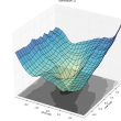
One way to find the optimal parameters is simply ‘exhaustive search’, evaluating the cost function over a full range of quantised parameter combinations and selecting the minimum. Visualising the cost surface produced is insightful; Figure 1 presents a 2 degree-of-freedom example for images related by pan-tilt camera rotation.

Figure 1: Example 2DoF image alignment cost function for pan-tilt camera rotation, with a clear minimum and smooth bowl.

 

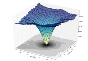
The clear bowl shape of this surface shows that we can do something much more efficient than exhaustive search as long as we start from a set of parameters close enough to correct alignment by following the gradient to the minumum.

3.2 Lucas-Kanade Algorithm

In LK alignment [12], at each iteration we use the gradient of the cost function in Equation 1 with respect to the warp parameter vector ${{\mathbf{p}}}$, and determine a parameter update $\Delta{{\mathbf{p}}}$ which takes us closer to the minimum of the function.

A more efficient version of this algorithm, which allows for pre-computation of the system Jacobian and Hessian was proposed in [3]. The trick consists of swapping the roles of the reference and template image and optimising for an update warp composed with the current warp estimate. The modified cost function has the form:

$$\Delta{{\mathbf{p}}}=\operatornamewithlimits{arg\ min}_{\Delta{{\mathbf{p}}}}\sum_{x}\lVert{{\mathtt{I}}}_{t}({{\mathtt{W}}}({{\mathbf{x}}};\Delta{{\mathbf{p}}}))-{{\mathtt{I}}}_{r}({{\mathtt{W}}}({{\mathbf{x}}};{{\mathbf{p}}}))\rVert^{2}~{},$$ (2)

with the following update rule:

$${{\mathtt{W}}}({{\mathbf{x}}};{{\mathbf{p}}})\leftarrow{{\mathtt{W}}}({{\mathbf{x}}};{{\mathbf{p}}})\circ{{\mathtt{W}}}({{\mathbf{x}}};\Delta{{\mathbf{p}}})^{-1}$$ (3)

Linearizing Equation 2 leads to a closed form solution:

$$\Delta{{\mathbf{p}}}=\left({\sum_{{\mathbf{x}}}{{\mathtt{J}}}^{T}{{\mathtt{J}}}}\right)^{-1}\sum_{{\mathbf{x}}}{{\mathtt{J}}}^{T}{{\mathbf{r}}}~{},$$ (4)

where:

$${{\mathtt{J}}}=-\nabla{{\mathtt{I}}}_{t}\frac{d{{\mathtt{W}}}({{\mathbf{x}}},{{\mathbf{p}}})}{d{{\mathbf{p}}}}\bigg{|}_{{{\mathbf{p}}}=0}$$ (5)

$${{\mathbf{r}}}={{\mathtt{I}}}_{r}({{\mathtt{W}}}({{\mathbf{x}}},{{\mathbf{p}}}))-{{\mathtt{I}}}_{t}({{\mathbf{x}}})$$ (6)

The shape of the convergence basin heavily depends on the image content: amount and type of texture and ambiguities present in the image. Since the cost landscape is usually locally convex in vincinity of the real translation, a good initialization is required for the optimization to successfuly converge to the correct solution.

3.3 Coarse-to-Fine Alignment

To increase the size of the convergence basin, the original image can be smoothed using Gaussian blur, which simplifies the cost surface through removing the details in the image [11]. The Gaussian smoothed image is usually downsampled since it does not cause loss of information and reduces the number of pixels to be processed. Since a pixel in the downsampled image corresponds to multpile pixels in the original image, the distance between the two is shortened, which increases the size of the basin of convergence. For the same reason, the accuracy of the alignment performed on smaller version of the images is also reduced.

The common approach is to start the optimization using highly downsampled and blurred images to obtain an initial estimate and refine it using progressively more detailed versions of the images. This can be perceived as a pyramid of degraded versions of the image.

4 Replacing the Pyramid with CNN Feature Maps

Outputs of the convolutions in standard classification CNN’s form a pyramid similar to the ones used in RGB based LK image alignment (Figure 2). Consecutive layers of such pyramid encode increasingly more semantic information, starting from simple geometrical filters in the first layers, leading to more complex concepts.

Each level of the pyramid takes the form of a multi-channel image (tensor), where each channel contains responses to a certain learned convolutional filter. We propose to align the volumes in a coarse-to-fine manner, starting from the highest, low resolution layers and progressing down to the lower, geometrical layers to refine alignment.

Figure 2: A comparison between a Gaussian pyramid (left) and proposed conceptual pyramid (right).

 

Section 4.1 presents the process of extracting the feature pyramid out of an input RGB image. Following this, Section (4.2) describes how standard Lucas-Kanade alignment can be applied to the proposed representation.

4.1 Feature Extraction

Figure 3: A pyramid is created using successive learned convolutions, just as in a standard CNN classification network. We have used VGG-16 for our experiments

 

The pyramid is created through applying successive convolutions followed by a nonlinear activation function, with occasional downsampling, very much like in standard CNN’s. The weights for convolutions are trained for an image classification task. Although we believe that any classification CNN could be used in our method, we have only tested weights from VGG-16 classification network from [21]. The network consists of 13 layers of convolutions. Figure 3 presents the architecture of this network.

4.2 Volume Alignment

For aligning volumes we use the inverse compositional cost function formulation described in Section 3.2:

$$\sum_{{\mathbf{x}}}\lVert{{\mathbf{e}}}_{{\mathbf{x}}}(\Delta{{\mathbf{p}}};{{\mathbf{p}}})\rVert^{2}=\sum_{{\mathbf{x}}}\lVert{{\mathtt{V}}}_{t}({{\mathtt{W}}}({{\mathbf{x}}};\Delta{{\mathbf{p}}}))-{{\mathtt{V}}}_{r}({{\mathtt{W}}}({{\mathbf{x}}};{{\mathbf{p}}}))\rVert^{2}$$ (7)

Similar to normal images, we define a volume of depth $N$ as a function: ${{\mathtt{V}}}:\mathbb{R}^{2}\rightarrow\mathbb{R}^{N}$. In order to solve for the parameter update $\Delta p$, one first need to calculate the Jacobian and Hessian of this nonlinear Least Squares System:

$${{\mathtt{J}}}_{{\mathbf{x}}}=\frac{\partial{{\mathbf{e}}}_{{\mathbf{x}}}}{\partial\Delta{{\mathbf{p}}}}=\begin{bmatrix}\frac{\partial e_{{{\mathbf{x}}},1}}{\partial\Delta{{\mathbf{p}}}}\\ \vdots\\ \frac{\partial e_{{{\mathbf{x}}},N}}{\partial\Delta{{\mathbf{p}}}}\end{bmatrix}=\begin{bmatrix}{{\mathtt{J}}}_{{{\mathbf{x}}},1}\\ \vdots\\ {{\mathtt{J}}}_{{{\mathbf{x}}},N}\end{bmatrix}$$ (8)

$$\begin{split}{{\mathtt{H}}}:=\sum_{{\mathbf{x}}}{{\mathtt{J}}}_{{\mathbf{x}}}^{T}{{\mathtt{J}}}_{{\mathbf{x}}}&=\sum_{{\mathbf{x}}}\left[{{\mathtt{J}}}_{{{\mathbf{x}}},1}^{T}\dots{\mathtt{J}}_{{{\mathbf{x}}},N}^{T}\right]\begin{bmatrix}{{\mathtt{J}}}_{{{\mathbf{x}}},1}\\ \vdots\\ {{\mathtt{J}}}_{{{\mathbf{x}}},N}\end{bmatrix}=\\ &=\sum_{{\mathbf{x}}}\sum_{c=1}^{N}{{\mathtt{J}}}_{{{\mathbf{x}}},c}^{T}{{\mathtt{J}}}_{{{\mathbf{x}}},c}\end{split}$$ (9)

$$\begin{split}{{\mathbf{b}}}:=\sum_{{\mathbf{x}}}{{\mathtt{J}}}_{{\mathbf{x}}}^{T}{{\mathbf{e}}}_{{\mathbf{x}}}&=\sum_{{\mathbf{x}}}\left[{{\mathtt{J}}}_{{{\mathbf{x}}},1}^{T}\dots{\mathtt{J}}_{{{\mathbf{x}}},N}^{T}\right]\begin{bmatrix}{{\mathbf{e}}}_{{{\mathbf{x}}},1}\\ \vdots\\ {{\mathbf{e}}}_{{{\mathbf{x}}},N}^{T}\end{bmatrix}=\\ &=\sum_{{\mathbf{x}}}\sum_{c=1}^{N}{{\mathtt{J}}}_{{{\mathbf{x}}},c}^{T}{{\mathbf{e}}}_{{{\mathbf{x}}},c}\end{split}$$ (10)

The update is calculated using the normal equations:

$$\Delta{{\mathbf{p}}}={{\mathtt{H}}}^{-1}{{\mathbf{b}}}$$ (11)

In order to perform alignment in real-time over big volumes we have implemented the optimization on GPU using NVIDIA CUDA. Each computational thread calculates per-pixel values, which are later reduced to single matrices using Equations 9 and 10.

5 Live Spherical Mosaicing

Figure 4: An example spherical panorama produced by tracking the camera rotation using CNN features

 

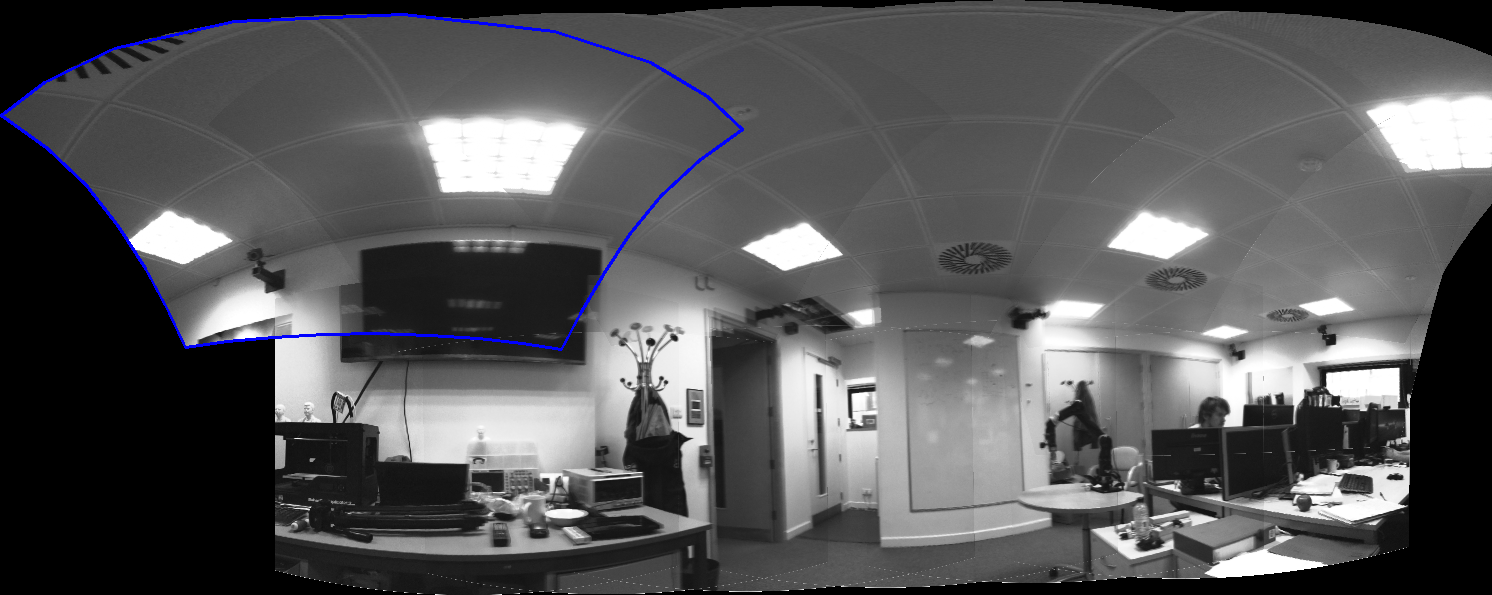
In order to test tracking using the proposed representation, we have developed a real-time spherical mosaicing system similar to [10]. It tracks purely rotational camera movement and produces a keyframe map, which is rendered into a spherical panorama. For purely rotational camera motion, the homography between two camera frames with intrinsic matrix ${{\mathtt{K}}}$, separated by rotation described by matrix ${{\mathtt{R}}}$ is given by: ${{\mathtt{K}}}{{\mathtt{R}}}{{\mathtt{K}}}^{-1}$ [6]. Therefore, the generative warp function from Section 3.1 has the form:

$${{\mathtt{W}}}({{\mathbf{x}}};{{\boldsymbol{\omega}}})=\pi({{\mathtt{K}}}{{\mathtt{R}}}({{\boldsymbol{\omega}}}){{\mathtt{K}}}^{-1}\dot{{\mathbf{x}}})~{},$$ (12)

where $\dot{{\mathbf{x}}}$ is the homogenized pixel location ${{\mathbf{x}}}$, and $\pi$ is the projection function. We parametrize the incremental rotation ${{\mathtt{R}}}({{\boldsymbol{\omega}}})$ with ${{\boldsymbol{\omega}}}\in R^{3}$. The incremental rotation described by vector ${{\boldsymbol{\omega}}}$ is mapped to the ${\mathfrak{so}(3)}$ group elements via [4]:

$${{\mathtt{R}}}({{\boldsymbol{\omega}}})=\exp({{\boldsymbol{\omega}}}^{\times})~{}.$$ (13)

The final cost function to be optimized takes the form:

$$\sum_{x}||{{\mathtt{V}}}_{t}(\pi({{\mathtt{K}}}{{\mathtt{R}}}({{\boldsymbol{\omega}}}){{\mathtt{K}}}^{-1}\dot{{\mathbf{x}}})-{{\mathtt{V}}}_{r}({{\mathtt{K}}}{{\mathtt{R}}}{{\mathtt{K}}}^{-1})||^{2}~{}.$$ (14)

The keyframe map is projected onto a final compositioning surface. We use spherical projection, which projects each keyframe onto a unit sphere, which is later unrolled into a 2D surface for viewing. An example mosaic produced by our system is presented in Figure 4. We use an image of size $224\times 224$ to extract features and align all of the levels.

The system runs in real-time 15-20 frames per second using the whole pyramid. Extraction of 13 layers of convolutional features takes around 1 ms per frame. Copying the data from GPU takes 10ms, which can be avoided by further modifications to the software. Time spent on performing the alignment depends on the number of iterations performed at different levels and usually is around 40–60ms.

6 Results

We present experiments which compare the performance of image alignment for our CNN pyramid with raw RGB and dense SIFT pyramids. For all tests we use our 3D camera rotation tracker described in Section 5. We consider that robustness is the most important factor in camera tracking, and therefore use the size of basin of convergence as our performance measure in the main results in Section 6.1.

We also investigate the possibility of improving the results and reducing the computational overhead through selecting the most valuable feature maps in Section 6.2.

6.1 Robust, long-term tracking

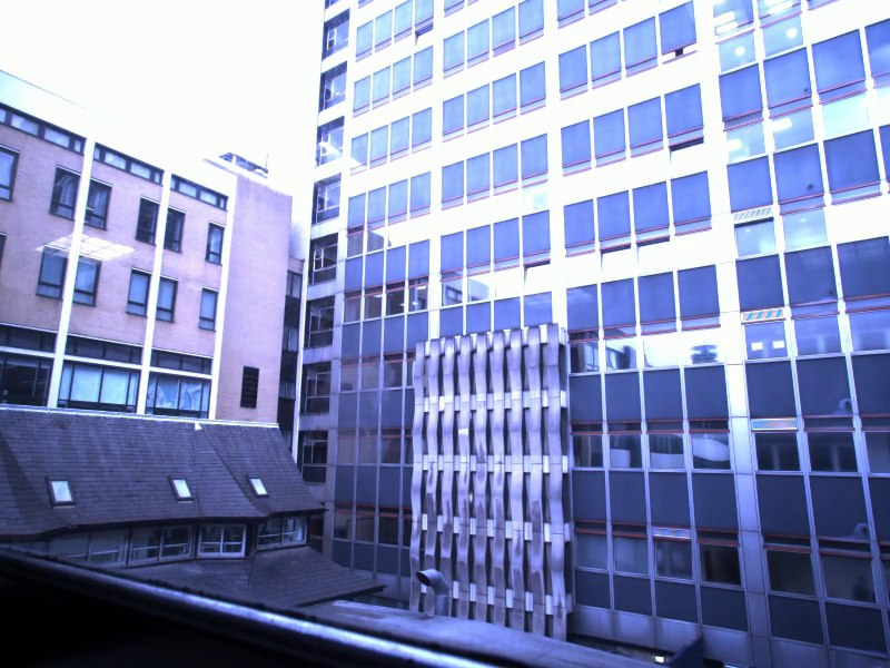
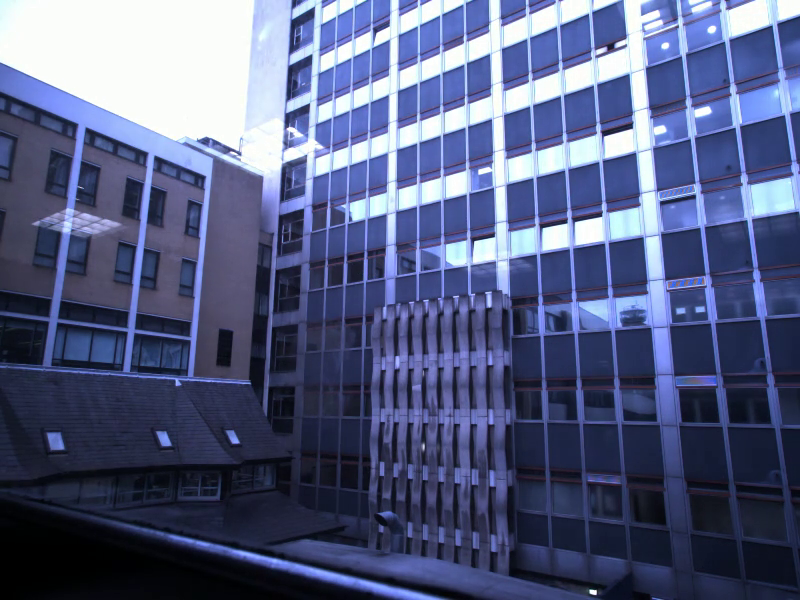
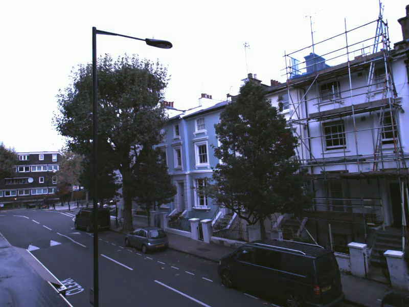
In order to test the robustness of the proposed representation in long-term tracking scenarios, three time-lapse sequences from a static camera have been captured showcasing real-world changing lighting conditions. The videos cover 8–10 hours of outdoor scenes, and have been sub-sampled into 2 minute clips.

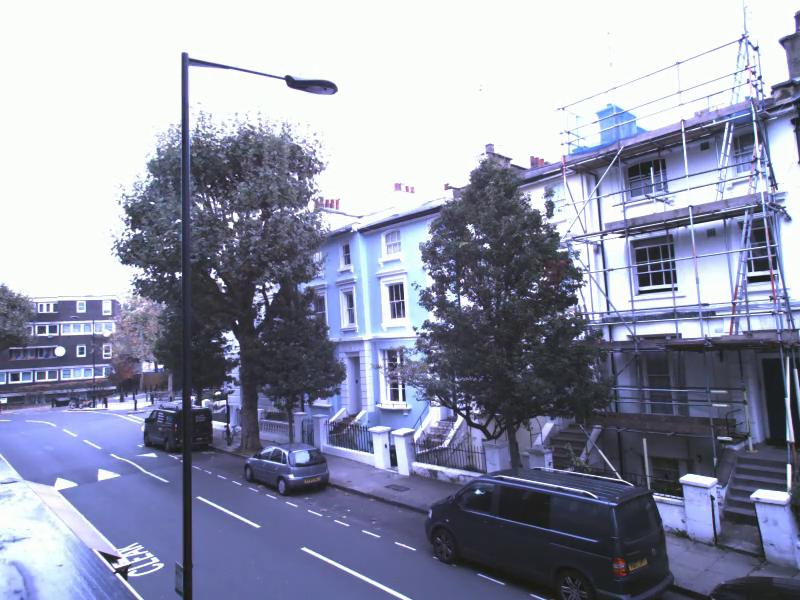
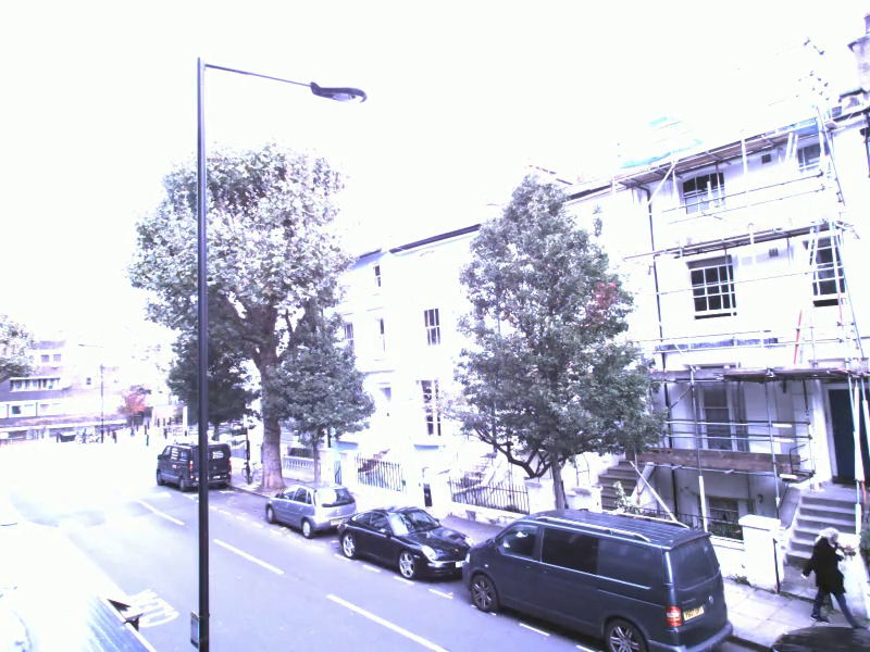
In our tests we focus on two of the captured sequences – window and home. The first features a highly specular scene which undergoes major and irregular lighting changes throughout the day with no major outliers. The home sequence shows a relatively busy street with frequent outliers. This sequence contains less specular surfaces, the observed illumination changes have more a global character.

We have selected three snapshots from each of these sequences containing different lighting conditions, and evaluated the area of the convergence basin while trying to align each possible pair of frames. To serve as a baseline comparison, we also present the results of alignment using RGB (RGB) and dense SIFT features (SIFT).

In order to measure the size of the convergence basin, we segment the parameter space into a regular grid and initialize the Lucas-Kanade algorithm at each point. Next, we perform the optimization for 1000 iterations and inspect the final result. We find that when convergence is successful, the final accuracy is generally good, and therefore define that if the tracking result is within 0.07 radians of ground truth, we mark the tested point as belonging to the convergence basin. The marked points are next used to calculate the total area of the convergence basin.

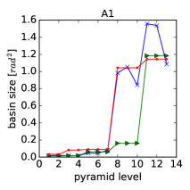
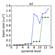
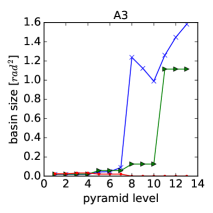
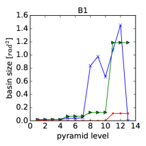
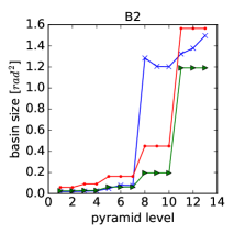
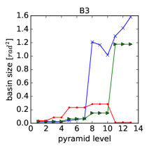
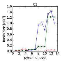
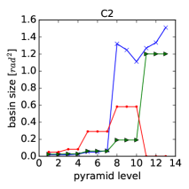
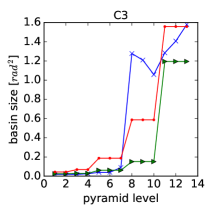
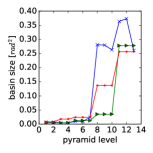
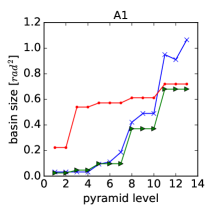
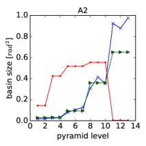
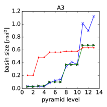
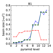
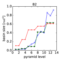
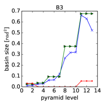
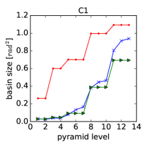
The results are presented in Figures 5 and 8. Five pyramids levels of SIFT and RGB have been used in the tests to compare with the proposed CNN pyramid. The missing values were duplicated in the plots so that it is possible to easily compare the convergence basin areas of the corresponding image resolutions (e.g. RGB/SIFT level 5 corresponds to CONV levels 11–13). Note that the LK alignment results are not symmetric with regard to which image is used as the template and which as the reference, as only the gradient of the template image is used, which might have impact on performance under varying lighting conditions and blur.

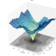
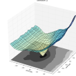
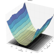
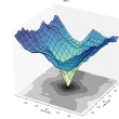
For frames from the window dataset (Figure 5), all of the methods have a sensible basin of convergence on the diagonal, where the images used for alignment are identical. For more challenging, off-diagonal pairs, such as A2, A3 or B3, the RGB cost function fails to provide a minimum in the correct spot, while SIFT and CONV still have wide, comparable convergence basins. One of the failure cases is showcased in more detail in Figure 6. The proposed CONV method seems to excel at higher levels, which are believed to have more semantic meaning.

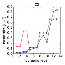
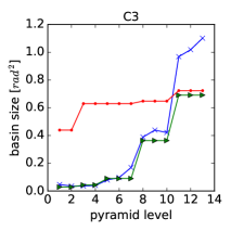
In the second, home sequence (Figure 8) RGB performs better, possibly due to the global character of the illumination changes. It still fails when the lighting changes significantly (pair C2,B3). Similar to the previous sequence, the proposed method performs at least as well as SIFT and better than RGB at the highest levels of pyramid.

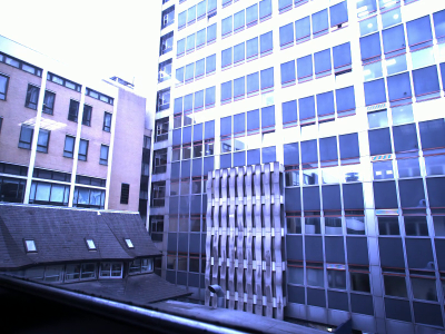
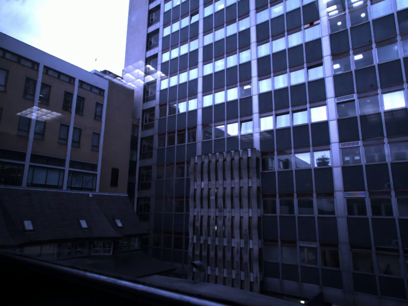
To evaluate how the proposed solution handles image blurring, we have tested it with an alignment problem of an image with a heavily blurred version of itself. Figure 7 presents the reference and template images used in this test, selected cost landscape plots of RGB, CONV and SIFT and a comparison of basin sizes. We can see that all methods are robust to blur, with our proposed method providing the best results at the highest pyramid levels. It provides a steady, wide basin of convergence at the top pyramid levels regardless of the lighting conditions and blur.

Figure 5: Comparison of sizes of convergence basins for aligning pairs of images with different lighting conditions (sampled from the window sequence). Each array cell presents convergence basins areas of RGB (red), SIFT (green) and CONV (blue) at different pyramid levels. The left column and top row images are used in LK as template and reference, respectively.

 

Figure 6: Cost landscape plots and convergence basin areas of different methods for aligning an image with a blurred version of itself. From left: template image, reference image, RGB cost landscape, SIFT cost landscape, CONV cost landscape, comparison of convergence basin areas (RGB: red, SIFT: green, CONV: blue).

 

Figure 7: Cost landscape plots and calculated convergence basin areas of different methods for aligning an image with a blurred version of itself. From left: template image, reference image, RGB cost landscape, SIFT cost landscape, CONV cost landscape, comparison of convergence basin areas (RGB: red, SIFT: green, CONV: blue).

 

Figure 8: Comparison of sizes of convergence basins for aligning pairs of images with different lighting conditions (sampled from the home sequence). Each array cell presents convergence basins areas of RGB (red), SIFT (green) and CONV (blue) at different pyramid levels. Left and top images are used in LK as template and reference, respectively.

 

6.2 Reducing the Number of Features

The results presented so far are based on aligning all of the CNN feature maps produced at each pyramid level jointly. One clear disadvantage of this approach is computational cost: the amount of work which needs to be done at each alignment iteration to calculate a difference is proportional to the number of features. It is apparent from any inspection of the features generated by a CNN that there is a lot of redundancy in feature maps, with many looking very similar, and therefore it seemed likely that it is possible to achieve similar or better results through selection of a percentage of features. Here we perform experiments to compare a random selection with simple criteria based on measures of texturedness and stability.

In standard Lucas-Kanade, the size of the convergence basin depends highly on image content. For example, a vertical stripe can only be used to detect horizontal translation; the lack of vertical gradient makes it impossible to determine the movement in this direction. In order to correctly regress the camera pose, a strong gradient in both feature directions is required. As in Shi and Tomasi’s classic ‘Good Features to Track’ paper [19], we measure the texturedness of a feature based on its structure tensor:

$${{\mathtt{G}}}_{f}=\sum_{{{\mathbf{x}}}\in{{\mathtt{I}}}_{f}}\begin{bmatrix}g_{x}^{2}&g_{x}g_{y}\\ g_{x}g_{y}&g_{y}^{2}\end{bmatrix},$$

where $I_{f}$ is the activation map of the feature in response to a certain input image. We use the smallest eigenvalue of matrix ${{\mathtt{G}}}_{f}$ as a comparable single score.

The other factor to consider is stability. Most valuable features provide stable activations that change only due to changes in camera pose. Features that react to objects that are likely to change their location, or lighting changes, are undesirable. We measure the instability of a feature $f$ by calculating the average sum of squared differences (SSD) between activations obtained from images of the test sequence to the ones extracted from the first image and warped to the current camera frame:

$$s_{f}=\frac{1}{N-1}\sum_{i=2}^{N}\sum_{{{\mathbf{x}}}}\lVert({{\mathtt{I}}}_{f}^{1}({{\mathtt{W}}}({{\mathbf{x}}};{{\boldsymbol{\omega}}}))-{{\mathtt{I}}}_{f}^{i}({{\mathbf{x}}})\rVert^{2}.$$

Averages of these two scores have been calculated across frames of three video sequences — two timelapses and one hand tracking sequence. We have selected and evaluated several subsets of features of varying size that have the optimal texturedness and stability. To assess their robustness, we again use the size of convergence basin as a measure. Twelve challenging (outliers, varying lighting conditions) image pairs sampled from our recorded sequences have been used in the evaluation.

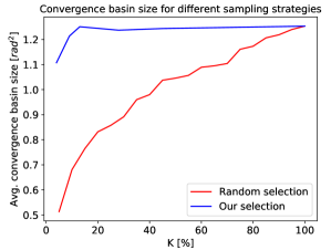
Figure 9 compares the average convergence basin size achieved with the features selected with our proposed approach with a baseline of using random selections. Random tests were performed in a range of 5–100% subsampling, with a step of 5%. Each sampled subset was tested 20 times against all twelve image pairs. We see very strongly that the features selected using our simple criteria give excellent tracking performance when they are much fewer than the whole set; while the performance of the randomly chosen features tails off much faster. This promises more sophisticated ways of learning ideal feature sets in the future.

Figure 9: Average convergence basin size obtained by using our proposed selection process (blue) and random sampling (red), for different sampling percentage. Results were evaluated using twelve image pairs representing the most challenging conditions (outliers, lighting variations).

 

7 Conclusions

We have shown that substituting the image pyramid in standard Lucas Kanade dense alignment with a hierarchy of feature maps generated by a standard VGG trained for classification straightforwardly gives much improved tracking robustness with respect to large lighting changes.

While this is immediately a neat and convenient method for tracking, we hope that it opens the door to further research on new representations for dense mapping and tracking which lie in between raw pixel values and object-level models. What levels of representation are needed in dense SLAM in order actually to achieve tasks such as detecting a change in an environment? A clear next step would be to investigate the performance of m-estimators on the CNN features to gate out outliers. Might we expect to see that whole semantic regions which had moved or changed could be masked out from tracking?

We imagine that a dense 3D model will be painted with smart learned feature texture for tracking and updating, rather than the raw pixel values of systems like DTAM [15].

References

- [1] P. Agrawal, J. Carreira, and J. Malik. Learning to see by moving. In Proceedings of the International Conference on Computer Vision (ICCV), 2015.
- [2] E. Antonakos, J. Alabort-i Medina, G. Tzimiropoulos, and S. P. Zafeiriou. Feature-based Lucas-Kanade and active appearance models. IEEE Transactions on Image Processing, 24(9):2617–2632, 2015.
- [3] S. Baker and I. Matthews. Lucas-Kanade 20 years on: A unifying framework: Part 1. International Journal of Computer Vision (IJCV), 56(3):221–255, 2004.
- [4] E. Eade. Lie groups for computer vision, 2014.
- [5] P. Fischer, A. Dosovitskiy, E. Ilg, P. Häusser, C. Hazırbaş, V. Golkov, P. van der Smagt, D. Cremers, and T. Brox. FlowNet: Learning Optical Flow with Convolutional Networks. In ICCV, 2015.
- [6] R. Hartley and A. Zisserman. Multiple View Geometry in Computer Vision. Cambridge University Press, second edition, 2004.
- [7] A. Hermans, G. Floros, and B. Leibe. Dense 3d semantic mapping of indoor scenes from rgb-d images. In Proceedings of the IEEE International Conference on Robotics and Automation (ICRA), 2014.
- [8] H. Hirschmüller. Evaluation of Cost Functions for Stereo Matching. In Proceedings of the IEEE Conference on Computer Vision and Pattern Recognition (CVPR), 2007.
- [9] A. Kendall, M. Grimes, and R. Cipolla. Convolutional networks for real-time 6-dof camera relocalization. CoRR, 2015.
- [10] S. J. Lovegrove and A. J. Davison. Real-Time Spherical Mosaicing using Whole Image Alignment. In Proceedings of the European Conference on Computer Vision (ECCV), 2010.
- [11] B. D. Lucas and T. Kanade. An Iterative Image Registration Technique with an Application to Stereo Vision. In Proceedings of the International Joint Conference on Artificial Intelligence (IJCAI), 1981.
- [12] B. D. Lucas and T. Kanade. Optical Navigation by the Method of Differences. In Proceedings of the International Joint Conference on Artificial Intelligence (IJCAI), pages 981–984, 1985.
- [13] W. Luo, A. G. Schwing, and R. Urtasun. Efficient deep learning for stereo matching. In CVPR2016, 2016.
- [14] J. McCormac, A. Handa, A. Davison, and S. Leutenegger. SemanticFusion: Dense 3D semantic mapping with convolutional neural networks. In Proceedings of the IEEE International Conference on Robotics and Automation (ICRA), 2017.
- [15] R. A. Newcombe, S. Lovegrove, and A. J. Davison. DTAM: Dense Tracking and Mapping in Real-Time. In Proceedings of the International Conference on Computer Vision (ICCV), 2011.
- [16] P. Perona and J. Malik. Scale space and edge detection using anisotropic diffusion. IEEE Transactions on Pattern Analysis and Machine Intelligence (PAMI), 12(7):629–639, 1990.
- [17] R. F. Salas-Moreno, R. A. Newcombe, H. Strasdat, P. H. J. Kelly, and A. J. Davison. SLAM++: Simultaneous Localisation and Mapping at the Level of Objects. In Proceedings of the IEEE Conference on Computer Vision and Pattern Recognition (CVPR), 2013.
- [18] Sergey Zagoruyko and Nikos Komodakis. Learning to compare image patches via convolutional neural networks. CoRR, 2015.
- [19] J. Shi and C. Tomasi. Good Features to Track. In Proceedings of the IEEE Conference on Computer Vision and Pattern Recognition (CVPR), 1994.
- [20] K. Simonyan, A. Vedaldi, and A. Zisserman. Deep inside convolutional networks: Visualising image classification models and saliency maps. arXiv preprint arXiv:1312.6034, 2013.
- [21] K. Simonyan and A. Zisserman. Very Deep Convolutional Networks for Large-Scale Image Recognition. In Proceedings of the International Conference on Learning Representations (ICLR), 2015.
- [22] J. Valentin, S. Sengupta, J. Warrell, A. Shahrokni, and P. Torr. Mesh Based Semantic Modelling for Indoor and Outdoor Scenes. In Proceedings of the IEEE Conference on Computer Vision and Pattern Recognition (CVPR), 2013.