Stochastic population dynamics in spatially extended predator-prey systems

Abstract

Spatially extended population dynamics models that incorporate demographic noise serve as case studies for the crucial role of fluctuations and correlations in biological systems. Numerical and analytic tools from non-equilibrium statistical physics capture the stochastic kinetics of these complex interacting many-particle systems beyond rate equation approximations. Including spatial structure and stochastic noise in models for predator-prey competition invalidates the neutral Lotka–Volterra population cycles. Stochastic models yield long-lived erratic oscillations stemming from a resonant amplification mechanism. Spatially extended predator-prey systems display noise-stabilized activity fronts that generate persistent correlations. Fluctuation-induced renormalizations of the oscillation parameters can be analyzed perturbatively via a Doi–Peliti field theory mapping of the master equation; related tools allow detailed characterization of extinction pathways. The critical steady-state and non-equilibrium relaxation dynamics at the predator extinction threshold are governed by the directed percolation universality class. Spatial predation rate variability results in more localized clusters, enhancing both competing species’ population densities. Affixing variable interaction rates to individual particles and allowing for trait inheritance subject to mutations induces fast evolutionary dynamics for the rate distributions. Stochastic spatial variants of three-species competition with ‘rock-paper-scissors’ interactions metaphorically describe cyclic dominance. These models illustrate intimate connections between population dynamics and evolutionary game theory, underscore the role of fluctuations to drive populations toward extinction, and demonstrate how space can support species diversity. Two-dimensional cyclic three-species May–Leonard models are characterized by the emergence of spiraling patterns whose properties are elucidated by a mapping onto a complex Ginzburg–Landau equation. Multiple-species extensions to general ‘food networks’ can be classified on the mean-field level, providing both fundamental understanding of ensuing cooperativity and profound insight into the rich spatio-temporal features and coarsening kinetics in the corresponding spatially extended systems. Novel space-time patterns emerge as a result of the formation of competing alliances; e.g., coarsening domains that each incorporate rock-paper-scissors competition games.

1 Introduction and historical overview

1.1 Introduction: population dynamics

For the purpose of this topical review, we shall view population dynamics as the study of (classical) interacting particle systems typically involving a number of different species, and their time evolution [1, 2, 3, 4, 5]. Population dynamics is most deeply rooted in ecology, where biologists and mathematicians have been investigating the dynamics of interacting animal, plant, or microbial species for centuries [6], via observations, theoretical considerations, and more recently by means of experiments in engineered, controlled environments. However, its principles as well as basic mathematical and computational tools have been successfully applied to an extremely diverse range of fields, such as the study of (bio-)chemical reactions [7], genetics [8], laser physics [9], economics [10], epidemiology, and the analysis of cancerous growths [11], to list but a few. It has hence become a foundational subfield of non-equilibrium statistical physics. In recent years, population dynamics has become a crucial tool to investigate the fundamental puzzle of the emergence and stabilization of biodiversity, and to seek means to preserve the latter in endangered and besieged ecosystems.

In this review, we chiefly focus our attention on the population dynamics of spatially extended systems. While non-spatial and well-mixed systems already exhibit intriguing properties, the explicit inclusion of spatial degrees of freedom that allow the propagation and mutual invasion of species may lead to the appearance of fascinating spatio-temporal patterns that include activity fronts, traveling waves, and spiral structures characteristic of excitable media [12, 13]. While the deterministic nature of mean-field equations, with the possible extension to spatially extended systems via the inclusion of, e.g., diffusive spreading, already yields important insights into the dynamics of competing populations, the explicit incorporation of stochasticity can fundamentally change and renormalize the behavior of a system of interacting species. We will therefore devote a substantial part of this brief overview to the discussion of random fluctuations in addition to spatio-temporal correlations induced by the underlying stochastic kinetics, and their consequences to species stability, model robustness, and dynamical pattern formation in coupled non-linear population models.

In particular, the description of species interactions via stochastic chemical reaction processes intrinsically includes internal reaction noise. In the case of the basic Lotka–Volterra (LV) two-species predator-prey system, stochastic models exhibit long-lived but ultimately decaying oscillations, already contradicting the classical picture of neutral population cycles. These features transcend the mean-field type mass-action treatment, and their theoretical analysis allows deep insights into the role of fluctuations on species survival as well as the formation of intriguing spatio-temporal patterns in spatially extended systems. Such stochastic interacting and reacting particle models can be elegantly studied via individual-based Monte Carlo simulations, i.e., stochastic cellular automata, uncovering intriguing spatio-temporal features such as predator-prey activity fronts that are induced and stabilized by the intrinsic reaction noise. Going beyond simulations, the Doi–Peliti framework enables a mapping of the (chemical) master equation to a Liouville operator formulation that encodes the reaction processes by means of (bosonic) creation and annihilation operators. Employing well-established tools from quantum many-particle physics and quantum or statistical field theory in turn allows qualitative insights as well as quantitative treatments beyond straightforward linear approximations, e.g., addressing the renormalization through non-linear stochastic fluctuations of observables such as the population oscillation frequencies, their relaxations, and characteristics pattern wavelengths.

In order to set the scene and to put this review into broader context, we start with a brief overview of the historical background and important experimental work over the last two centuries. The subsequent section 2 focuses on the classic LV model, the role of intrinsic ‘reaction’ noise and its treatment via stochastic chemical processes, its spatial extension via placement on a regular lattice, the emergence of spatio-temporal patterns, spatial heterogeneity, critical properties near the predator extinction threshold, and the inclusion of evolutionary dynamics. This is followed by section 3 on cyclic three-species systems, where we discuss the paradigmatic rock-paper-scissors and May–Leonard models. In section 4, we extend our attention to general systems with more than three species and extended food networks, discussing the formation of both spatio-temporal patterns and emerging species alliances. Finally, we end this overview in section 5 with our conclusions and outlook on the future evolution of this field.

1.2 Historical overview

The study of population dynamics looks back over two centuries of history in the mathematical and ecological sciences. Malthus’ growth law [10] is widely regarded as the ‘first law of population ecology’. In this work, he debated that the exponential human population growth is incompatible with linear growth of food resources and argued for population controls to be put in place. However, unchecked infinite exponential growth is obviously unphysical, hence the exponential law was later amended by Verhulst to construct the logistic growth model [14]. Almost ninety years later, Pearl applied the logistic equation, which had been derived independently by Lotka [15], to model population growth in the US [16]. In 1926, Volterra introduced a simple model describing the effects of two interacting species in close proximity [17], and used this model to explain oscillations of fish populations (and the resulting catch volumes) in the Adriatic sea as observed by D’Ancona [6]. Lotka independently introduced the same set of rate equations in his work on chemical oscillations and physical biology [18, 4].

Volterra argued that the growth rate of the prey population density $b$, given as $b^{-1}db/dt$, should be a decreasing function of the predator density $a$ and greater than zero when the predator density is zero. Conversely, the predator growth rate $a^{-1}da/dt$ should increase with the prey count, but be negative when $b=0$. The simplest coupled set of non-linear differential equations following these arguments represents the LV competition model that describes the population densities of predators $a$ and prey $b$:

$$\frac{da(t)}{dt}=a(t)\left[\lambda b(t)-\mu\right],\quad\frac{db(t)}{dt}=b(t)\left[\sigma-\lambda a(t)\right],$$ (1)

where $t$ denotes the (continuous) time. The parameters $\lambda$, $\mu$, and $\sigma$ describe the phenomenolgical predation, predator death, and prey reproduction rates, respectively. This set of coupled ordinary differential equations gives rise to characteristic, undamped, non-linear oscillations, see figure 1. Very similar techniques were also used to model warfare [6].

However, the LV equations (1) are rather simplistic, with the most obvious flaw being the unchecked growth of the prey in the absence of predators. In the 1930s, Gause proposed a generalized mathematical model in which the rate parameters effectively become response functions of the respective species, allowing more realistic control of populations compared to the original LV model [19, 20, 21]. In his 1936 note, Kolmogorov published an even more general set of equations governing a system of two interacting predator and prey species [22],

$$\frac{da(t)}{dt}=\alpha(a,b)\,a(t)\,,\quad\frac{db(t)}{dt}=\beta(a,b)\,b(t)\,.$$ (2)

He argued that the response functions $\alpha$ and $\beta$ should decrease with increasing predator density $a$, i.e,. $\partial_{a}\alpha(a,b)<0$ and $\partial_{a}\beta(a,b)<0$, which is a broadly accepted fact in theoretical ecology [21], and makes Kolmogorov’s model much more realistic than the LV model. Nevertheless, the LV model has remained quite popular owing to its simplicity and the low number of free parameters. We will introduce the LV model and discuss its spatially extended and stochastic counterpart in detail in section 2.

The models we discussed so far are concerned with the mean population densities only, neglecting the influence of random fluctuations on the populations. The study of the stochastic aspects of population dynamics (or indeed epidemiology) likely began with McKendrick in 1926, where, in his seminal paper, he derived the probabilistic master equation for the Susceptible-Infected-Recovered (SIR) model [23, 4, 24]. The SIR system represents the most basic model of epidemiology to describe the spread of an infection through a susceptible population, and still serves as an extremely popular paradigmatic model in the current literature.

In 1937, MacLulich analyzed time series data on the populations of lynx and snowshoe hare in Canada [25], first published by Hewitt [26]. These data were inferred from the volume of fur traded via the Hudson Bay Company going back to the early nineteenth century. Strikingly, both lynx and hare populations show multi-year recurrent spikes, and thus exhibit the signature non-linear oscillatory cycles of the LV system. Therefore this time series data is considered as one of the classic examples for LV oscillations and an early validation of this rather simplistic model.

In the 1950s, spatial aspects of predator-prey population dynamics were first considered. Huffaker created an experimental spatially extended lattice for two competing species of mites [27]. He arranged oranges in a two-dimensional array such that mites can traverse between them and use the oranges as a habitat. In this system, the mite species Eotetranychus sexmaculatus serves as the prey, while the mite Typhlodromus occidentalis plays the role of predator. Huffaker counted the number of mites of either species over time on each orange in the lattice arrangement. His data indeed also displayed the characteristic oscillations associated with the LV model, in addition to the striking spatio-temporal patterns formed by the mite population distribution. Huffaker’s mite universes also contained heterogeneity in the form of rubber balls replacing oranges, thereby showing that spatial heterogeneity and species motility stabilize the coexistence of the two competing species. The oranges and rubber balls can be considered to be interacting patches in a metapopulation model for spatially extended predator-prey dynamics.

Based on an observation by Wright that in spread-out areas larger than the average migration distance, populations occur in essentially isolated patches, with individuals migrating between neighboring patches, Kimura introduced the stepping stone model for population genetics [28, 29]. This model, which is equivalent to the well-known voter model, explained the local genetic characteristics based on the size of population patches [30]. Durrett and co-workers later extended this to understand the effects of local mutations [30].

In his seminal paper on evolutionary genetics, Moran proposed a process for neutral drift and genetic fixation in populations of fixed size [31, 32]. In this model, the population of alleles A or B can change via the death of a randomly chosen individual and its replacement by the offspring of a second randomly chosen individual. The Moran model can then be used to predict the fixation times and probabilities of alleles A and B, depending on population size and initial populations. It can be extended to account for evolutionary selection when one of the two alleles is assigned a higher reproduction probability consistent with a fitness advantage.

In the late 1960s and the 1970s, spatial aspects of population dynamics gained traction in the theoretical ecology community. For example, Levins derived principles for the control of invading insect pests using simple spatial models [33]. Hastings considered a two-species predator-prey system in which prey can migrate to empty areas and predators can subsequently invade prey patches [34]. This all-to-all connected system exhibits stable predator-prey coexistence phases. Meanwhile, May showed that randomly assembled species interaction networks become less stable with growing size and connectivity according to random matrix theory and linear stability analysis [1], an intriguing result as it seemingly contradicts the common belief that higher diversity generically leads to more stable ecosystems.

In their seminal 1973 essay, Maynard Smith and Price laid the groundwork for the application of game theory concepts to population dynamics and to the study of evolutionary theory [35]. Crucially, Maynard Smith also popularized the ‘rock-paper-scissors’ (RPS) game in which three species interact cyclically via LV terms [36]. May and Leonard published their important modified cyclic interaction model in 1975 [37]. The crucial difference between these two model variants is that in the RPS model consumed prey change identity and are converted into their respective predator species, with the total population number remaining conserved, while in the May–Leonard model (MLM) the competition is more indirect, and unconstrained by net population conservation. Perhaps the most prominent example of cyclic interaction in nature are the mating strategies of the Californian side-blotched lizard, observed to obey the rules of the RPS game by Sinervo and Lively [38]. We discuss cyclic games in detail in section 3.

In 1957, Kerner developed a statistical mechanics framework for interacting species based on the LV model. He made the observation that the LV equations admit a Liouville theorem and exhibit a conserved quantity [39]. In the early 1990s, more researchers began applying the methods of statistical physics to study population dynamics in spatially extended systems. Dunbar showed that in one dimension, the LV equations with diffusive spreading support travelling wave solutions [40] akin to Fisher–Kolmogorov waves. Matsuda et al. developed a lattice model based on the LV interaction rules and analyzed its evolutionary stability and the emergence of altruism using a pair approximation method [41]. Satulovsky and Tomé developed a stochastic model for predator-prey dynamics on a square lattice and investigated its phase diagram using dynamical mean-field theory and computer simulations [42]. They observed absorbing states as well as a coexistence regime with local oscillatory behavior. Boccara, Roblin, and Roger studied a similar stochastic lattice system and also found that overall species densities tended to stable values in the coexistence phase, while local oscillations still persisted [43]. Similar numerical and analytical studies were also performed for cyclically competing species [44, 45].

2 Stochastic lattice Lotka–Volterra predator-prey models

2.1 Classical mean-field rate equations

We have already introduced the classical mean-field Lotka–Volterra rate equations (1) in section 1, and discussed their most important shortcomings. One may view these coupled ordinary non-linear differential equations as the well-mixed, deterministic limit for time evolution of the mean populations of a system of two interacting predator and prey species. The microscopic and more general Lotka–Volterra reaction rules from which equations (1) derive are given by:

$$B\stackrel{{\scriptstyle\sigma}}{{\rightarrow}}B+B\,,\quad A\stackrel{{\scriptstyle\mu}}{{\rightarrow}}\emptyset\,,\quad A+B\stackrel{{\scriptstyle\lambda^{\prime}}}{{\rightarrow}}A+A\,.$$ (3)

The prey $B$ reproduce with rate $\sigma>0$; the predators $A$ spontaneously die with rate $\mu>0$; and upon encountering each other in their immediate vicinity, both species may interact with (microscopic) predation rate $\lambda^{\prime}>0$, whereupon the participating prey is consumed while the predator generates one offspring. On a hypercubic $d$-dimensional lattice with lattice constant $a_{0}$, the mean-field continuum reaction rate in eqs. (1) is connected with its microscopic counterpart via $\lambda=a_{0}^{d}\lambda^{\prime}$. The above three reaction rules are to be interpreted as continuous-time stochastic processes, and the discreteness in individual numbers is important near the absorbing states, where either the predator population $A$ goes extinct, leaving ever multiplying prey $B$, or even both species disappear. Neither of the processes (3) allows the system to leave these absorbing states, affirming the irreversibility and hence non-equilibrium character of this stochastic kinetics. We remark that host-pathogen systems are modeled essentially by the same set of non-linear reactions [46, 47, 48].

If implemented on a lattice, one may in addition allow for nearest-neighbor (or more long-range) particle hopping processes with rate $D^{\prime}$ (with associated continuum diffusivity $D=a_{0}^{d}D^{\prime}$); alternatively, random particle exchange has been implemented. If one imposes the restriction that each lattice site can at most be occupied by a single individual, prey birth entails that the offspring particle be placed on an adjacent position; likewise, the predation reaction must then involve two neighboring lattice sites. These processes then automatically generate diffusive population spreading. As we shall see below, spatial as well as temporal correlations turn out to be important features in the LV system that often crucially influence the ensuing population dynamics. Nevertheless, much insight can be gathered by beginning with an analysis of the mean-field description (1) of the LV model. Note that these coupled rate equations entail a mass action factorization of a two-point correlation function that encodes the likelihood of predators and prey meeting each other at given location at the same time into a simple product of their average uniform densities $a$ and $b$; hence spatio-temporal correlations are manifestly ignored in this approximate and, in general, rather crude description.

Straightforward linear stability analysis of the rate equations (1) yields three stationary states [49, 4, 50]: (1) the linearly unstable (for $\sigma>0$) absorbing total population extinction state $(a=0,b=0)$; (2) a linearly unstable (for $\lambda>0$) predator extinction and Malthusian prey explosion state $(a=0,b\to\infty)$; and (3) the marginally stable species coexistence fixed point $(a=\sigma/\lambda,b=\mu/\lambda)$. Expanding in fluctuations about this fixed point, one obtains within the linear approximation neutral cycles with purely imaginary stability matrix eigenvalues, i.e., undamped population oscillations with characteristic frequency $\omega_{0}=\sqrt{\sigma\mu}$. Indeed, the full non-linear coupled differential LV equations (1) give rise to a conserved first integral

$$K=\lambda\left[a(t)+b(t)\right]-\sigma\ln a(t)-\mu\ln b(t).$$ (4)

This in turn implies closed orbits in phase space spanned by the two population densities, which therefore each display characteristic non-linear oscillations with the unrealistic feature that both predator and prey densities return precisely to their initial values after each cycle [4, 50], see figure 1.

Figure 1: Left: Characteristic non-linear LV mean-field oscillations of predator (red) and prey (blue) populations over time obtained through numerical integration of the rate equations (1) with parameters $\sigma=\mu=\lambda=0.5$ and initial densities $a(0)=0.1$, $b(0)=1$. Right: The oscillatory dynamics implies closed orbits (neutral cycles) in population density phase space (reproduced with permission from Ref. [51]).

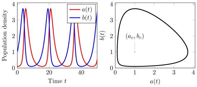
The presence of neutral cycles in the deterministic LV model (1) moreover hints at the lack of robustness in this approximate mean-field description with respect to even minor modifications. Indeed, model alterations typically induce a negative real part for the stability matrix eigenvalues in the species coexistence phase, representing attenuated kinetics that ultimately takes the populations to stationary fixed-point densities. One biologically relevant LV variant posits a finite carrying capacity $\rho$ for the prey [4] mimicking either limited food resources or direct intra-species competition (e.g., $B+B\rightarrow B$ with rate $\sigma/\rho$ [52]). On the mean-field level, the prey population rate equation in (1) is then to be replaced with

$$\frac{db(t)}{dt}=\sigma\,b(t)\left[1-\frac{b(t)}{\rho}\right]-\lambda a(t)b(t)\ .$$ (5)

This restricted LV model sustains again three stationary states [50]: (1) total extinction $(a=0,b=0)$; (2’) predator extinction and prey saturation at its carrying capacity $(a=0,b=\rho)$; and (3’) predator-prey coexistence $(a=\sigma(1-\mu/\rho\lambda)/\lambda,b=\mu/\lambda)$. This coexistence state only exists, and then is linearly stable, if the predation rate exceeds the threshold $\lambda>\lambda_{c}=\mu/\rho$. Otherwise, fixed point (2’) is stable, and the predator species is driven toward extinction. In the two-species coexistence regime, the stability matrix eigenvalues become

$$\epsilon_{\pm}=-\frac{\sigma\mu}{2\lambda\rho}\left[1\pm\sqrt{1-\frac{4\lambda\rho}{\sigma}\left(\frac{\lambda\rho}{\mu}-1\right)}\right].$$ (6)

Consequently, if the eigenvalues $\epsilon_{\pm}$ are both real, i.e., $\sigma>\sigma_{s}=4\lambda\rho(\lambda\rho/\mu-1)>0$, or $\mu/\rho<\lambda<\lambda_{s}=\mu(1+\sqrt{1+\sigma/\mu})/2\rho$, the neutral cycles of the unrestricted model (1) turn into a stable node; alternatively, if $\sigma<\sigma_{s}$ or $\lambda>\lambda_{s}$, fixed point (3’) becomes a stable focus, and is approached in phase space via a spiraling trajectory. In the former situation, both predator and prey densities approach their stationary values exponentially, in the latter case through damped population oscillations.

Spatial structures can be accounted for within the mean-field framework through extending the rate equations (1), (5) to a set of coupled partial differential equations for local predator and prey densities $a({\vec{x}},t)$ and $b({\vec{x}},t)$, and heuristically adding diffusive spreading terms:

$$\frac{\partial a({\vec{x}},t)}{\partial t} = \left(D_{A}\nabla^{2}-\mu\right)a({\vec{x}},t)+\lambda\,a({\vec{x}},t)\,b({\vec{x}},t)\ ,$$

$$\frac{\partial b({\vec{x}},t)}{\partial t} = \left(D_{B}\nabla^{2}+\sigma\right)b({\vec{x}},t)-\frac{\sigma}{\rho}\,b({\vec{x}},t)^{2}-\lambda\,a({\vec{x}},t)b({\vec{x}},t)\ ;$$ (7)

note that these reaction-diffusion equations still assume weak correlations as encoded in the mass action factorization in the predation terms. In one dimension, equations (2.1) permit explicit travelling wave solutions of the form $a(x,t)={\bar{a}}(x-vt)$, $b(x,t)={\bar{b}}(x-vt)$ that describe a predator invasion front from the coexistence phase described by homogeneous fixed point (3’) into a region occupied only by prey [40, 53, 4]. An established lower bound for the front propagation speed is $v>\sqrt{4D_{A}(\lambda\rho-\mu)}$ [54].

2.2 Non-spatial stochastic LV systems

The dominant role of stochastic fluctuations in the LV model that are due to the internal reaction noise, is already apparent in non-spatial or zero-dimensional (purely on-site) ‘urn model’ realizations. The system is then fully described by a (local) stochastic master equation that governs the time evolution of the configurational probability $P(n,m;t)$ to find $n$ predators $A$ and $m$ prey $B$ at time $t$ through a balance of gain and loss terms. For the set of reactions (3), the master equation reads [55, 50, 52]

$$\frac{\partial P(n,m;t)}{\partial t} = \sigma\left[(m-1)\,P(n,m-1;t)-m\,P(n,m;t)\right]$$

$$+ \mu\left[(n+1)\,P(n+1,m;t)-n\,P(n,m;t)\right]$$

$$+ \lambda^{\prime}\left[(n-1)(m+1)\,P(n-1,m+1;t)-nm\,P(n,m;t)\right]\ .$$

It should first be noted that as $t\to\infty$, the system will inevitably reach the completely empty absorbing state, where both species have become extinct. For reasonably abundant populations, however, both direct and refined continuous-time Monte Carlo simulations utilizing Gillespie’s algorithm [56] display erratic but persistent population oscillations over effectively many generations; as one would expect, their remarkably large amplitude scales roughly like the square-root of the mean total particle number in the system [55]. McKane and Newman elucidated the physical mechanism behind these persistent random oscillations by means of a van Kampen system size expansion [57], which essentially maps the stochastic LV system with finite prey carrying capacity $\rho$ to a non-linear oscillator driven by white noise with frequency-independent correlation spectrum. On occasion, these random kicks will occur at the resonance frequency ($\omega_{0}=\sqrt{\sigma\mu}$ in linear approximation) and thus incite high-amplitude population density excursions away from the mean-field coexistence fixed point (3’). For sufficiently large predation rate $\lambda^{\prime}$, the subsequent relaxation follows a spiral trajectory in phase space, i.e., damped oscillatory kinetics.

The discrete small number fluctuations or demographic noise also strongly impacts the survival time near an absorbing extinction state [58, 59]. These can be treated in the framework of large-deviation theory based on the master equation or, more directly, through the equivalent Doi–Hamiltonian that encodes the associated generating function [60], for example by means of a ‘semi-classical’ WKB-type approach; Ref. [61] provides an excellent up-to-date review. The mean extinction time in the stochastic non-spatial LV model (2.2) is a relevant example of the intriguing influence of demographic noise in a mean-field setting: By exploiting the existence of the mean-field constant of motion (4), Parker and Kamenev performed a semi-classical analysis of the Fokker–Planck equation derived from (2.2) and devised a method to average demographic fluctuations around the LV mean-field orbits [58, 62]. They thus showed that the mean number of cycles prior to extinction scales as $N_{S}^{3/2}/N_{L}^{1/2}$, where $N_{S}$ and $N_{L}$ respectively denote the characteristic sizes of the smaller and larger of the predator or prey sub-populations, and determined the mean extinction time in terms of the number of cycles. This result means that extinction typically occurs faster when the number $N_{L}$ of individuals of the most abundant species increases.

The reverse problem of understanding the large spikes in the populations of predators and prey can be described by turning the classic LV equations (1) into stochastic differential equations via the introduction of multiplicative noise in the prey birth. This problem can be rewritten in the form of a Fokker–Planck–Kolmogorov equation for the probability distribution for the sizes of the predator and prey populations, which can be solved exactly. The solutions indicate strong intermittent behavior with small population means and rare, large excursions of the population sizes when the noise levels are high, which are also observed in Monte Carlo simulations [63].

2.3 Coexistence in spatially extended stochastic Lotka–Volterra systems

The stochastic LV model (3) can be implemented on a $d$-dimensional lattice, usually with periodic boundary conditions to minimize edge effects, in a straightforward manner via individual-based Monte Carlo update rules. One may either allow arbitrarily many predator or prey particles per site, or restrict the site occupancy representing a finite local carrying capacity. For example, one detailed Monte Carlo algorithm on a two-dimensional square lattice with site restrictions (at most a single particle allowed per site) proceeds as follows [50, 64]:

• Select a lattice occupant at random and generate a random number $r$ uniformly distributed in the range $[0,1]$ to perform either of the following four possible reactions (with probabilities $D^{\prime}$, $\sigma$, $\mu$, and $\lambda^{\prime}$ in the range $[0,1]$):

• If $r<1/4$, select one of the four sites adjacent to this occupant, and move the occupant there with probability $D^{\prime}$, provided the selected neighboring site is empty (nearest-neighbor hopping).

• If $1/4\leq r<1/2$ and if the occupant is an $A$ particle, then with probability $\mu$ the site will become empty (predator death, $A\rightarrow\emptyset$).

• If $1/2\leq r<3/4$ and if the occupant is an $A$ particle, choose a neighboring site at random; if that selected neighboring site holds a $B$ particle, then with probability $\lambda^{\prime}$ it becomes replaced with an $A$ particle (predation reaction, $A+B\rightarrow A+A$).

• If $3/4\leq r<1$ and if the occupant is a $B$ particle, randomly select a neighboring site; if that site is empty, then with probability $\sigma$ place a new $B$ particle on this neighboring site (prey offspring production, $B\rightarrow B+B$).

Notice that even for $D^{\prime}=0$, the particle production processes on neighboring lattice sites effectively induce spatial population spreading. One Monte Carlo step is considered completed when on average each particle present in the system has been picked once for the above processes. If arbitrarily many individuals of either species are allowed on each lattice site, all reactions can be performed locally, but then hopping processe need to be implemented explicitly to allow diffusive propagation (an explicit Monte Carlo simulation algorithm is, e.g., listed in Ref. [65]).

Alternatively, one can use event-driven simulation schemes such as the Gillespie or kinetic Monte Carlo algorithm [56]. A Gillespie algorithm equivalent to the sequential update Monte Carlo scheme described above would be:

1. Set time $t=0$ and choose initial state.

2. List all possible reactions that change the state of the system:

   • the number of possible prey reproduction events $N_{\sigma}$, i.e. the number of $B$ particles with empty neighboring sites;

   • the number of possible predator death events $N_{\mu}$, i.e. the number of $A$ particles on the lattice;

   • the number of possible predation events $N_{\lambda}$, i.e. the number of neighboring pairs of $A$ and $B$ particles;

   • the number of possible diffusion events $N_{D}=\sum_{i=1}^{N}n_{i}$, where $n_{i}=0,\ldots,4$ is the number of empty adjacent sites of particle $i$, and $N$ the total number of particles on the lattice.

3. Calculate the reaction propensities of each event $R_{\sigma}=\sigma N_{\sigma}$, $R_{\mu}=\mu N_{\mu}$, $R_{\lambda}=\lambda^{\prime}N_{\lambda}$ and $R_{D}=D^{\prime}N_{D}$. Choose an event type $i$ at random with the probability weighed according to the respective propensities.

4. Carry out a randomly chosen event of the given type in the list assembled in step (ii).

5. Advance time by $\Delta t=-\ln(r)/R_{i}$ where $r\in(0,1]$ is a uniformly distributed random number.

6. Continue with step (ii).

The Gillespie algorithm requires no choice of time step length and thus provides exact trajectory samples from the solution of the master equation. It is also rejection-free because every event results in a reaction and is thus more efficient than a sequential update algorithm. However, the Gillespie algorithm (and its variants, see Ref. [66] for a good overview) can be challenging to implement due to the complexity involved in calculating the reaction propensities. It has been successfully applied to study the LV model and the RPS model in both spatial [67, 68, 69, 70] and non-spatial contexts [71, 58, 59].

Figure 2: Early time evolution for the population density of predators $a(t)$ (red), prey $b(t)$ (blue), and the mean-field first integral $K(t)$ (green) in a stochastic two-dimensional lattice LV model with $1024\times 1024$ sites (periodic boundary conditions, no occupation number restrictions) from two single runs that both started with a random particle distribution with reaction rates (a) $\sigma=0.1$, $\mu=0.2$, and $\lambda=1.0$, and (b) $\sigma=0.4$, $\mu=0.1$, and $\lambda=1.0$ (reproduced with permission from Ref. [65]).

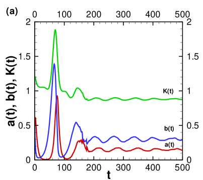
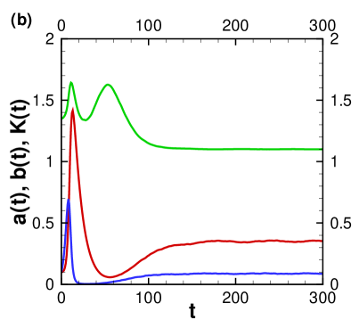
Computer simulations based on similar Monte Carlo algorithms of sufficiently large stochastic LV systems, thus avoiding full population extinction, invariably yield long-lived erratic population oscillations and a stable predator-prey coexistence regime [42, 43, 72, 73, 74, 75, 76, 77, 78, 79, 80, 50, 65, 64]. Two typical simulation runs on a two-dimensional square lattice without site occupation restrictions, starting with particles that are randomly distributed in the system, are shown in figure 2. Both predator and prey densities display damped oscillatory kinetics, with the oscillation frequency and the attenuation depending on the prescribed reaction rates. In stark contrast with the mean-field rate equation solutions (see figure 1), there are no neutral cycles, and instead one clearly observes relaxation towards (quasi-)stationary population densities representing a stable coexistence state. The quantity $K(t)$ (4), representing the conserved rate equations’ first integral, becomes time-dependent and oscillates along with the population densities. The oscillation amplitude scales as the inverse square-root of the lattice size, hinting at the presence of spatially separated and largely independent (non-linear) oscillators in the system [72, 74, 75, 77, 79, 80, 50], each subject to local noise-induced resonant amplification [55].

Figure 3: Left: space-time plot for a stochastic LV model simulation on a chain with $250$ sites (and periodic boundary conditions), initial densities $a(0)=1=b(0)$, and rates $\sigma=0.5$, $\mu=0.5$, and $\lambda=0.3$; the temporal evolution is displayed vertically downward, the colors blue and red indicate the presence of prey and predator particles, respectively, purple marks sites occupied by both species, and black pixels denote empty sites. At $t=0$ the system is well-mixed; over time, clusters of prey particles form and grow; predators subsequently invade prey clusters, often removing them completely. Right: snapshots from a two-dimensional stochastic lattice LV simulation with $250\times 250$ sites (periodic boundary conditions, multiple occupations allowed), $a(0)=0.01$, $b(0)=1$, $\sigma=0.1$, $\mu=0.9$, and $\lambda=1$. Here, the prey community survives an early predator invasion (at $t=17$ MCS), followed by prey recovery and proliferation due to predator scarcity ($t=30$ MCS). New predator fronts later invade a large prey cluster ($t=71$ MCS). Following transient oscillations, the system reaches a quasi-steady species coexistence state ($t=500$ MCS) characterized by smaller prey clusters and recurring predator invasions (reproduced with permission from Ref. [51]).

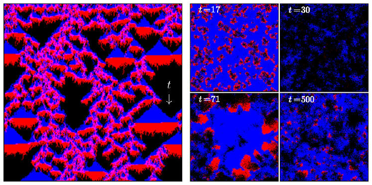
Inspection of successive temporal snapshots of the Monte Carlo data for the spatial population distributions and full movie visualizations [81, 50, 65, 82, 83, 51, 64] further illuminate the origin of the local population oscillations incited by the system-immanent stochasticity or internal reaction noise [84]. As shown in the space-time plot on the left panel of figure 3, quite complex temporal behavior emerges already in one dimension, with growing prey clusters suffering predator invasion from their boundaries and subsequent near-elimination, with the few surviving prey particles forming the nuclei for renewed growth spurts. This repetitive spatially correlated dynamics induces striking spatio-temporal patterns, and even more so in two dimensions; lattice snapshots for one example are depicted in the right panels of figure 3. Localized prey clusters are invaded and devoured by predators, who then starve and come close to extinction, until scarce survivors become the sources for radially spreading prey-predator fronts that subsequently merge and interact, giving rise to spatially separated local population oscillations. The characteristic LV activity fronts represent a proto-typical example for the more general non-equilibrium phenomenon of formation of noise-induced and -stabilized spatio-temporal patterns [85, 86]. For the LV system, these recurring fluctuating structures and the associated erratic oscillations are in fact quite robust against modifications of the microscopic reaction scheme, rendering the features of spatially extended stochastic LV systems remarkably universal. They only become suppressed in lattice simulations in $d>4$ spatial dimensions, or upon implementation of effective species mixing through fast particle exchange (‘swapping’) processes, whereupon the dynamics attains the characteristic signatures of the corresponding mean-field rate equation solutions [81].

Figure 4: equational-time correlation functions (a) $C_{AA}(x)$, (b) $C_{BB}(x)$, and (c) $C_{AB}(x)$, measured in stochastic LV simulations on a $1024\times 1024$ lattice, with rates $\sigma=0.1$, $\mu=0.1$, and different values of the predation rate $\lambda=0.5$ (blue), $0.75$ (green), and $1.0$ (red) (reproduced with permission from Ref. [65]).

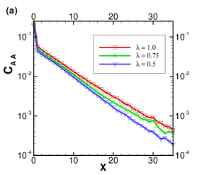
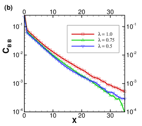
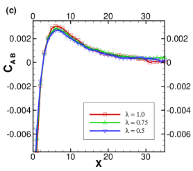
The Monte Carlo simulation data are of course amenable to a quantitative analysis of the emerging spatial and temporal correlations in stochastic lattice LV systems [50, 65]. Figure 4 displays the three static (equal-time) correlation functions $C_{\alpha\beta}(x)=\langle n_{\alpha}(x)\,n_{\beta}(0)\rangle-\langle n_{\alpha}(x)\rangle\,\langle n_{\beta}(0)\rangle$, with local occupation numbers $n_{\alpha}$ and species indices $\alpha,\beta=A,B$, i.e., the predator-predator and prey-prey correlators $C_{AA}(x)$ and $C_{BB}(x)$, as well as the two-species cross-correlations $C_{AB}(x)$, as function of distance $x$ in the predator-prey coexistence phase of a two-dimensional lattice with $1024\times 1024$ sites for fixed rates $\sigma,\mu$, but different values of $\lambda$. As is apparent from figures 4(a) and (b), both $C_{AA}(x)$ and $C_{BB}(x)$ are positive and decay exponentially $\sim e^{-|x|/\xi}$ with correlation lengths $\xi$ on the scale of a few lattice constants, which represents the typical width of the spreading population fronts. The predator-prey cross-correlations $C_{AB}(x)$ similarly decay at large distances from positive values, but naturally are negative (anti-correlated) at short $x$, since prey that approach too closely to predators may not survive the encounter. The maximum in figure 4(c) located at about six lattice constants indicates the mean spacing between the prey and following predator waves.

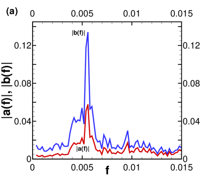
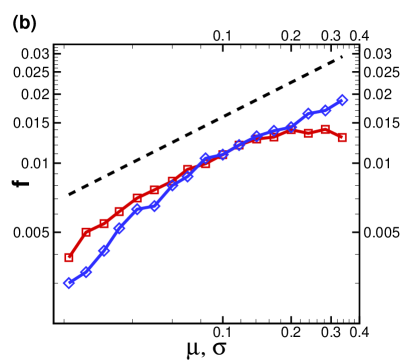
The characteristic oscillation frequency and damping are most efficiently and reliably determined through Fourier analysis of the density time series, $a(f)=\int e^{2\pi ift}\,a(t)\,dt$ for the predators (and similarly for the prey density $b$). As demonstrated in figure 5(a), the population density Fourier amplitudes display a marked peak, whose location can be identified with the oscillation frequency, while its half-width at half-maximum gives the attenuation rate or inverse relaxation time. The double-logarithmic plot of ensuing data measured for two-dimensional stochastic LV systems with various reaction rates shows that the functional dependence of the oscillation frequency on $\mu$ and $\sigma$ roughly follows the mean-field square-root behavior, yet with noticeable deviations as the ratio $\sigma/\mu$ deviates from $1$. However, the characteristic population oscillations in spatially extended stochastic LV models clearly occur at markedly lower frequencies, here reduced by a factor $\sim 2$ as compared with the linearized rate equation prediction.

The algorithm described above can be modified to introduce more complex interaction patterns. For example, Rozenfeld and Albano introduced the ability for prey to forego reproduction if predators are within a range $V_{H}$, and allowed for escape-pursuit via an interaction potential [87, 88]. This yields a phase in which self-sustained oscillatory behavior of the overall populations can be observed – even in the thermodynamic limit – based on dynamic percolation. This finding is in contrast to the above model in which oscillations are always decaying towards the coexistence fixed point.

Figure 5: (a) Fourier transforms $|a(f)|$ and $|b(f)|$ of the predator (red) and prey (blue) population density time series for a stochastic LV simulation run on a $1024\times 1024$ lattice with rates $\sigma=0.03$, $\mu=0.1$, and $\lambda=1.0$, as functions of frequency $f$. (b) Measured dependence of the characteristic peak frequencies in $|a(f)|$ and $|b(f)|$ on the rates $\sigma$ (red squares) and $\mu$ (blue diamonds), with the respective other rate held fixed at the value $0.1$ and $\lambda=1.0$, as obtained from simulation data on $1024\times 1024$ lattices up to time $t=20,000$; for comparison, the dashed black line shows the linearized mean-field oscillation frequency $f_{0}=\sqrt{\sigma\mu}/2\pi$ (reproduced with permission from Ref. [65]).

2.4 Doi–Peliti field theory and perturbative analysis

The remarkably strong renormalization of the characteristic population oscillation features through intrinsic stochastic fluctuations in spatially extended LV systems can be understood at least qualitatively through a perturbative computation based on a field theory representation of the master equation (2.2) as afforded by the powerful Doi–Peliti formalism (recent reviews are, e.g., provided in Refs. [89, 90, 60]). To this end, we permit an arbitrary number of predator and prey particles per site, $n_{i},m_{i}=0,1,\ldots,\infty$, but implement a growth-limiting pair annihilation reaction for the prey species, $B+B\rightarrow B$ with rate $\nu^{\prime}$. Since all stochastic reactions locally alter occupation numbers by integer values, it is convenient to introduce a bosonic ladder operator algebra $[a_{i},a_{j}]=0$, $[a_{i},a_{j}^{\dagger}]=\delta_{ij}$ for the predator species $A$, from which their particle number eigenstates $|n_{i}\rangle$ can be constructed, satisfying $a_{i}\,|n_{i}\rangle=n_{i}\,|n_{i}-1\rangle$, $a_{i}^{\dagger}\,|n_{i}\rangle=|n_{i}+1\rangle$, $a_{i}^{\dagger}\,a_{i}\,|n_{i}\rangle=n_{i}\,|n_{i}\rangle$. In the same manner, one proceeds with bosonic prey operators, and imposes $[a_{i},b_{j}]=0=[a_{i},b_{j}^{\dagger}]$. A general state vector is then defined as a linear combination of all particle number eigenstates, weighted with their configurational probabilities: $|\Phi(t)\rangle=\sum_{\{n_{i}\},\{m_{i}\}}P(\{n_{i}\},\{m_{i}\};t)\,|\{n_{i}\},\{m_{i}\}\rangle$. The master equation is then transformed into the (linear) time evolution equation $\partial|\Phi(t)\rangle/\partial t=-H\,|\Phi(t)\rangle$ with local reaction pseudo-Hamiltonian (Liouville operator)

$$\ H_{\rm reac}=-\sum_{i}\left[\mu\,\bigl{(}1-a_{i}^{\dagger}\bigr{)}\,a_{i}+\sigma\,\bigl{(}b_{i}^{\dagger}-1\bigr{)}\,b_{i}^{\dagger}\,b_{i}+\nu^{\prime}\,\bigl{(}1-b_{i}^{\dagger}\bigr{)}\,b_{i}^{\dagger}\,b_{i}^{2}+\lambda^{\prime}\,\bigl{(}a_{i}^{\dagger}-b_{i}^{\dagger}\bigr{)}\,a_{i}^{\dagger}\,a_{i}\,b_{i}\right].\$$ (9)

Nearest-neighbor hopping processes are similarly represented by

$$H_{\rm diff}=\sum_{<ij>}\left[D^{\prime}_{A}\,\bigl{(}a_{i}^{\dagger}-a_{j}^{\dagger}\bigr{)}\,\bigl{(}a_{i}-a_{j}\bigr{)}+D_{B}^{\prime}\,\bigl{(}b_{i}^{\dagger}-b_{j}^{\dagger}\bigr{)}\,\bigl{(}b_{i}-b_{j}\bigr{)}\right]\,.$$ (10)

In order to arrive at a continuum field theory representation, one follows the standard route in quantum many-particle physics to utilize coherent states, i.e., eigenstates of the annihilation operators with complex eigenvalues $\alpha_{i}$ and $\beta_{i}$: $a_{i}\,|\alpha_{i}\rangle=\alpha_{i}\,|\alpha_{i}\rangle$ and $b_{i}\,|\beta_{i}\rangle=\beta_{i}\,|\beta_{i}\rangle$, to construct a path integral for the time evolution of arbitrary observables in this basis,

$$\langle{\cal O}(t)\rangle\!\propto\!\int\!\prod_{i}\!d\alpha_{i}\,d\alpha_{i}^{*}\,d\beta_{i}\,d\beta_{i}^{*}\,{\cal O}(\{\alpha_{i}\},\{\beta_{i}\})\,\exp(-S[\alpha_{i}^{*},\beta_{i}^{*};\alpha_{i},\beta_{i};t])\,,\$$ (11)

with a statistical weight that is determined by the action

$$S[\alpha_{i}^{*},\beta_{i}^{*};\alpha_{i},\beta_{i}]=\sum_{i}\int dt\,\left[\alpha_{i}^{*}\,\frac{\partial\alpha_{i}}{\partial t}+\beta_{i}^{*}\,\frac{\partial\beta_{i}}{\partial t}+H(\alpha_{i}^{*},\beta_{i}^{*};\alpha_{i},\beta_{i})\right]\ .$$ (12)

Finally, the continuum limit is taken: $\sum_{i}\to a_{0}^{-d}\int d^{d}x$; where $a_{0}$ denotes the lattice constant, $\alpha_{i}(t)\to a_{0}^{d}\,a(\vec{x},t)$, $\beta_{i}(t)\to a_{0}^{d}\,b(\vec{x},t)$, $\alpha_{i}^{*}(t)\to{\hat{a}}(\vec{x},t)$, and $\beta_{i}^{*}(t)\to{\hat{b}}(\vec{x},t)$. Upon performing the field shifts ${\hat{a}}({\vec{x}},t)=1+{\tilde{a}}({\vec{x}},t)$, ${\hat{b}}({\vec{x}},t)=1+{\tilde{b}}({\vec{x}},t)$, and setting $\nu=a_{0}^{d}\nu^{\prime}=\sigma/\rho$, the action becomes explicitly

$$S[{\tilde{a}},{\tilde{b}};a,b]=\int\!d^{d}x\int\!dt\,\Biggl{[}{\tilde{a}}\,\Biggl{(}\frac{\partial}{\partial t}-D_{A}\,\nabla^{2}+\mu\Biggr{)}a+{\tilde{b}}\,\Biggl{(}\frac{\partial}{\partial t}-D_{B}\,\nabla^{2}-\sigma\Biggr{)}b$$

$$\quad\qquad\qquad\qquad\quad\ -\sigma\,{\tilde{b}}^{2}\,b+\frac{\sigma}{\rho}\,(1+{\tilde{b}})\,{\tilde{b}}\,b^{2}-\lambda\,(1+{\tilde{a}})\,({\tilde{a}}-{\tilde{b}})\,a\,b\,\Biggr{]}.$$ (13)

If it is interpreted as a Janssen–De Dominicis functional in a path integral representation for stochastic partial differential equations [60], it may be viewed equivalent to two coupled Langevin equations for complex fields

$$\frac{\partial a({\vec{x}},t)}{\partial t} = (D_{A}\nabla^{2}-\mu)\,a({\vec{x}},t)+\lambda\,a({\vec{x}},t)\,b({\vec{x}},t)+\zeta({\vec{x}},t)\ ,$$

$$\frac{\partial b({\vec{x}},t)}{\partial t} = (D_{B}\nabla^{2}+\sigma)\,b({\vec{x}},t)-\frac{\sigma}{\rho}\,b({\vec{x}},t)^{2}-\lambda\,a({\vec{x}},t)\,b({\vec{x}},t)+\eta({\vec{x}},t)\,.\$$ (14)

These resemble the reaction-diffusion equations (2.1) for (real) local particle densities, with additional Gaussian stochastic forcing with zero mean, $\langle\zeta\rangle=0=\langle\eta\rangle$, and the noise (cross-)correlations

$$\langle\zeta({\vec{x}},t)\,\zeta({\vec{x}}^{\prime},t^{\prime})\rangle=2\lambda\,a({\vec{x}},t)\,b({\vec{x}},t)\,\delta({\vec{x}}-{\vec{x}}^{\prime})\,\delta(t-t^{\prime})\ ,$$

$$\langle\zeta({\vec{x}},t)\,\eta({\vec{x}}^{\prime},t^{\prime})\rangle=-\lambda\,a({\vec{x}},t)\,b({\vec{x}},t)\,\delta({\vec{x}}-{\vec{x}}^{\prime})\,\delta(t-t^{\prime})\ ,$$

$$\langle\eta({\vec{x}},t)\,\eta({\vec{x}}^{\prime},t^{\prime})\rangle=2\sigma\,b({\vec{x}},t)\,\Bigl{[}1-b({\vec{x}},t)/\rho\Bigr{]}\,\delta({\vec{x}}-{\vec{x}}^{\prime})\,\delta(t-t^{\prime}),\,$$ (15)

which describe multiplicative noise terms that vanish with the particle densities, as appropriate for the presence of a fully absorbing state at $a=0=b$; similar Langevin equations were derived in Ref. [85] by means of a van Kampen system size expansion [57].

In the predator-prey coexistence regime, one proceeds by expanding the fields about their stationary values. Subsequent diagonalization of the resulting Gaussian (bilinear) action yields circularly polarized eigenmodes with dispersion $i\omega({\vec{q}})=\pm i\omega_{0}+\gamma_{0}+D_{0}q^{2}$ (for equal predator and prey diffusivities $D_{A}=D_{0}=D_{B}$) with ‘bare’ oscillation frequency $\omega_{0}^{2}=\sigma\mu(1-\mu/\lambda\rho)-\gamma_{0}^{2}$ and damping $\gamma_{0}=\sigma\mu/2\lambda\rho$, see eq. (6); note that $\gamma_{0}\to 0$ in the absence of site occupation restrictions or infinite carrying capacity $\rho$. One may then compute fluctuation corrections to the oscillation frequency, diffusion constant, and attenuation by means of a systematic perturbation expansion with respect to the non-linear predation rate $\lambda$; in fact, the effective expansion parameter turns out to be $(\lambda/\omega_{0})(\omega_{0}/D_{0})^{d/2}$ [52]. As observed in the computer simulations, first-order perturbation theory gives a downward renormalization for the characteristic frequency, which is particularly strong in dimensions $d\leq 2$ owing to the very weak (for large $\rho$) mean-field attenuation. The fluctuation corrections moreover appear largely symmetric in the rates $\sigma$ and $\mu$ and become enhanced as $\sigma\ll\mu$ or $\sigma\gg\mu$; both these features are also in accord with the Monte Carlo data, see figure 5(b). The diffusion rate is shifted upwards by the fluctuations, indicating faster front propagation. In contrast, the damping rate $\gamma$ is reduced; both these renormalizations facilitate instabilities towards spontaneous pattern formation that occur for $\gamma<0$ at wavenumbers $q<\sqrt{|\gamma|/D}$.

2.5 Predator species extinction threshold

Figure 6: Monte Carlo simulation trajectories for a stochastic LV model on a $1024\times 1024$ square lattice with periodic boundary conditions and restricted site occupancy (at most one particle allowed per site) in the predator-prey density phase plane ($a(t)+b(t)\leq 1$) with initial values $a(0)=b(0)=0.3$ (blue dot), fixed rates $\sigma=1.0$, $\mu=0.025$, and predation rates $\lambda=0.035$ (black): predator extinction phase; $\lambda=0.049$ (red): exponential relaxation to the quasi-stationary state just beyond the extinction threshold in the active coexistence phase; and $\lambda=0.250$ (green): deep in the two-species coexistence phase, with spiraling trajectories representing a damped oscillatory relaxation (adapted with permission from Ref. [64]).

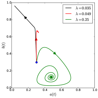
In the presence of site occupation number restrictions, stochastic lattice LV models feature a sharp continuous non-equilibrium phase transition that separates the two-species coexistence state from a prey-only phase wherein the predator species is driven to extinction [75, 78]. Different simulation trajectories in the population density phase plane obtained for varying values of the predation rate $\lambda$ are displayed in figure 6. At least qualitatively, these follow remarkably well the fixed-point analysis following eq. (6): For small predation efficiency, the predators die out, and the system reaches an absorbing state with prey proliferation. Just beyond this extinction threshold in the coexistence phase, both species quickly reach their asymptotic stationary densities through exponential relaxation; simulation snapshots or movies show localized predator clusters immersed in a ‘sea’ of abundant prey. For large predation rates, persistent damped population oscillations emerge, reflected in spiraling trajectories in the phase plane; in this situation, one observes complex spatio-temporal patterns induced by spreading and colliding prey-predator activity fronts [50, 84].

On quite general grounds, one expects the critical properties of non-equilibrium phase transitions from an active phase to an absorbing state to be described by the universality class of critical directed percolation, with directionality set along the time ‘direction’ [91, 92, 93, 94, 60]. In the absence of additional conservation laws and quenched spatial disorder, one expects this statement to be true even for multi-species systems [95]. It was thus surmised early on that the predator extinction transition in spatially extended LV models with restricted local carrying capacities is governed by the directed-percolation scaling exponents, and there now exists ample numerical evidence to support this statement [42, 43, 73, 74, 75, 76, 78, 80, 50, 64]. Indeed, once the predator species becomes sparse and the prey abundant, essentially uniformly filling the lattice, the predation reaction $A+B\rightarrow A+A$ may just happen everywhere and is effectively replaced by a spontaneous branching process $A\rightarrow A+A$; in conjunction with the decay processes $A\rightarrow\emptyset$ and $A+A\rightarrow A$ (reflecting again a locally restricted carrying capacity), one hence arrives at the basic stochastic processes defining directed percolation. Formally, considering fluctuations of the predator density near zero and of the prey density about $\rho$, one may directly map the Doi–Peliti action (2.4) for the near-threshold stochastic LV model onto Reggeon field theory

$$S[{\widetilde{\psi}},\psi]=\int d^{d}x\int dt\left[{\widetilde{\psi}}\left(\frac{\partial}{\partial t}+D\left(\tau-\nabla^{2}\right)\right)\psi-u\,{\widetilde{\psi}}\left({\widetilde{\psi}}-\psi\right)\psi\right]$$ (16)

that captures the universal scaling properties of critical directed percolation [96, 93, 60].

Figure 7: Left: Decay of the mean predator density (double-logarithmic plots) for a stochastic Lotka–Volterra model on a $1024\times 1024$ square lattice at the extinction threshold $\lambda_{c}=0.0416$ for $\sigma=1.0$ and $\mu=0.025$ and for both quasi-stationary (top, black) and random (lower curve, red dotted) initial configurations (data averaged over $2000$ independent simulation runs). For comparison, the predator density decay data are shown as well for $\lambda=0.0417$ (blue, active coexistence phase) and $\lambda=0.0415$ (orange, predator extinction phase). The inset shows the local effective decay exponent $\alpha_{\rm eff}(t)$. Right: Characteristic relaxation time $t_{c}$ near the critical point. Left inset: $t_{c}(\lambda_{2})$ after the system is quenched from a quasi-steady state at $\lambda_{1}=0.25>\lambda_{2}$ near $\lambda_{c}=0.0416$. (The different graphs indicate $t_{c}$ when $128000$, $64000$, $32000$, and $16000$ MCS elapsed after the quench; data averaged over $500$ runs.) Main panel: same data in double-logarithmic form. For $|\tau|=|(\lambda_{2}/\lambda_{c})-1|>0.1$, the different graphs collapse, yielding $z\,\nu=-1.208\pm 0.167$. Right inset: associated effective exponent $(z\,\nu)_{\rm eff}(\tau)$ that tends towards $z\,\nu\approx 1.3$ as $|\tau|\to 0$ (reproduced with permission from Ref. [64]).

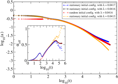
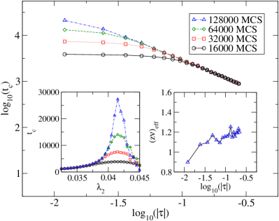
Examples for numerically determined dynamical critical properties at the LV predator extinction threshold $\lambda_{c}$ in a square lattice with $1024\times 1024$ sites are shown in figure 7 [64]: The predator density should decay algebraically according to $a(t)\sim t^{-\alpha}$, and upon approaching the transition, $\tau\sim\lambda-\lambda_{c}\to 0$, the characteristic relaxation time should display critical slowing down $t_{c}(\tau)\sim|\tau|^{-z\,\nu}$, with critical exponents $\alpha\approx 0.45$ and $z\nu\approx 1.295$ for directed percolation in two dimensions. The left panel in figure 7 depicts rather extensive simulation data for the critical predator density decay, starting from either random particle distributions, or following equilibration at higher predation rate, corresponding to a (quasi-)steady state in the coexistence region. The best estimate for the decay exponent here is $\alpha\approx 0.54$, but the asymptotic critical regime is only reached after $\sim 10^{5}$ MCS. As evident in the right panel of figure 7, data collapse for different time durations after the quench from the coexistence state ensues only for $|\tau|\geq 0.1$ in this system, giving $z\,\nu\approx 1.2$, but apparently extrapolating towards the directed-percolation value as $|\tau|\to 0$. Other characteristic signatures that can be examined in a straightforward manner in Monte Carlo simulations on reasonably small lattices include the expected power laws in the decay of the survival probability and the growth of the active-site number directly at the critical point [50].

Figure 8: Aging scaling plot (double-logarithmic) for the scaled predator density autocorrelation function $s^{b}\,C(t,s)$ as a function of the time ratio $t/s$ for various waiting times $s=100,200,500,1000,1500,2000$ MCS at the predator extinction critical point $\lambda_{c}=0.0416$ (data averaged over $1000$ independent runs for each value of $s$). The straight-slope section of the curves with waiting times $s\geq 1000$ MCS yields $\Lambda_{c}/z=2.37\pm 0.19$; the aging scaling exponent is found to be $b=0.879\pm 0.005$. Inset: effective exponent $-(\Lambda_{c}/z)_{\rm eff}(t)$ (reproduced with permission from Ref. [64]).

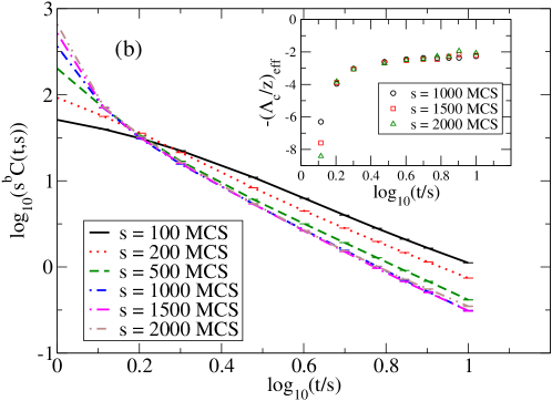
Universal dynamical critical behavior may also be accessed in studies of out-of-equilibrium relaxation. The system is then quenched from a fully disordered initial configuration to the critical point. Since the relaxation time diverges there, stationarity cannot be reached, and even in finite systems time translation invariance is broken during an extended time period. In this physical aging region, two-time autocorrelation functions satisfy the simple-aging dynamical scaling form [97]

$$C(t,s)=s^{-b}\,{\hat{C}}(t/s)\,,\quad{\hat{C}}(x)\sim x^{-\Lambda_{c}/z}\ .$$ (17)

As a consequence of the so-called rapidity reversal symmetry $\psi({\vec{x}},t)\leftrightarrow-{\widetilde{\psi}}({\vec{x}},-t)$ encoded in the Reggeon field theory action (16), the aging scaling exponents are linked to stationary dynamical critical exponents through the scaling relations $b=2\,\alpha$, $\Lambda_{c}/z=1+\alpha+d/z$ [93, 97], giving $b\approx 0.9$ and $\Lambda_{c}/z\approx 2.8$ in $d=2$ dimensions. Corresponding scaling plots for the predator density autocorrelation function for stochastic LV models at the critical point indeed obey equation (17) with $b\approx 0.88$ and $\Lambda_{c}/z\approx 2.37$ [64], as demonstrated in figure 8. Interestingly, these data require simulation runs for only $10^{4}$ MCS, an order of magnitude less than needed to (marginally) establish stationary dynamic scaling. Critical aging might thus provide a faster indicator for impending population collapse than critical slowing-down.

2.6 Random environmental influences versus demographic variability

Figure 9: Effect of spatial heterogeneity (environmental variability) governed by the width of the standard deviation of the predation rate distribution, determined for fixed $\sigma=0.5$ and $\mu=0.5$, on (a) the asymptotic mean population densities of predators (solid lines) and prey (dashed lines) compared to the mean-field prediction (dash-dotted line); (b) the relaxation time towards the (quasi-)steady state; (c) the intra-species correlation lengths as well as the typical separation distance between predators and prey; and (d) the front speed of spreading activity rings, measured for $\sigma=1$ and $\mu=0.2$ (reproduced with permission from Ref. [82]).

In spatially extended predator-prey models, an interesting question can be asked: How does spatial heterogeneity influence the population dynamics? In real ecosystems, there tend to exist spatial regions in which it is easier for prey to hide, while other parts of the system might be beneficial hunting grounds for predators. There might also be preferred breeding environments in which species profileration is enhanced, or more hazardous places in which the probability for species death is higher. Cantrell and Cosner looked at this question by linearizing a deterministic diffusive logistic equation and using the principal eigenvalue as a measure of environmental favorability [98, 99]. Spatial heterogeneity can be implemented by varying the rates governing the reaction processes between sites on the simulation lattice. For example, interesting boundary effects are found in the vicinity of interfaces separating active predator-prey coexistence regions from absorbing regions wherein the predators go extinct. The net predator flux across such a boundary induces a local enhancement of the population oscillation amplitude as well as the attenuation rate [100].

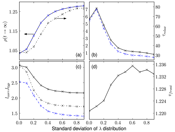
On the other hand, when the predation rates are treated as quenched random variables, affixed to the lattice sites and chosen from a truncated Gaussian distribution, remarkably the population densities of both predator and prey species are enhanced significantly beyond the baseline densities with homogeneous rates [82], see figure 9. The relaxation time into the steady state, as well as the inter- and intra-species correlation lengths decrease with growing rate variability, which is controlled by the standard deviation of the Gaussian distribution. The underlying microscopic mechanism behind these effects is the presence of lattice sites with particularly low and hence favorable reaction rates which act as prey proliferation sites. In contrast, heterogeneity in the prey reproduction and predator death rates does not significantly affect the species populations [82].

Figure 10: Distribution of predation efficencies at steady state, $\rho_{A,\infty}$ (predators) and $\rho_{B,\infty}$ (prey), in a predator-prey system with demographic variability and evolutionary dynamics for (a) finite correlation between the parent and offspring efficiencies, and (b) uniformly distributed efficiencies. The densities of both species do not fixate at extreme predation efficiencies (reproduced with permission from Ref. [83]).

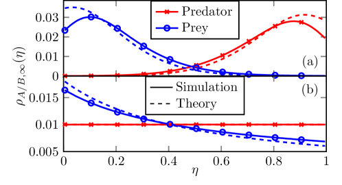
Compared with spatial heterogeneity and quenched randomness, demographic variability plays a different role: Reaction efficiencies of predators and prey, $\eta_{A}$ and $\eta_{B}$ respectively, become traits associated with individuals of both species [83] as opposed to fixed, population-based properties. During an inter-species predation reaction, these efficiencies are then used to construct an instantaneous reaction rate $\lambda$ from the arithmetic mean of the individuals’ $\eta_{A}$ and $\eta_{B}$, selecting for prey with low $\eta_{B}$ and predators with high $\eta_{A}$. Furthermore, individuals are assigned their efficiencies at birth, drawn from a truncated Gaussian distribution centered around the parent’s value of $\eta$. The ensuing coupled population and evolutionary dynamics of this system leads to an intriguing optimization of the efficiency distributions, shown in figure 10, which can also be approximated using an adapted multi-quasi-species mean-field approach [51]. Interestingly, the net effect on population densities of the evolutionary efficiency optimization is actually essentially neutral. Crucially, however, the mean extinction time in small systems is increased more than fourfold in the presence of such demographic variability [83, 51]. The optimization of efficiency distributions is reminiscent of co-evolutionary arms race scenarios: Yoshida et al. studied the consequences of rapid evolution on the predator-prey dynamics of a rotifer-algae system, using experiments and simulations via coupled non-linear differential equations [101, 102].

3 Cyclic dominance of three-species populations

Unraveling what underpins the coexistence of species is of fundamental importance to understand and model the biodiversity that characterizes ecosystems [103]. In this context, the cyclic dominance between competing species has been proposed as a possible mechanism to explain the persistent species coexistence often observed in Nature, see, e.g. Refs. [38, 104, 105, 106, 107]. In the last two decades, these observations have motivated a large body of work aiming at studying the dynamics of populations exhibiting cyclic dominance. The simplest and, arguably, most intuitive form of cyclic dominance consists of three species in cyclic competition, as in the paradigmatic rock-paper-scissors game (RPS) - in which rock crushes scissors, scissors cut paper, and paper wraps rock. Not surprisingly therefore, models exhibiting RPS interactions have been proposed as paradigmatic models for the cyclic competition between three species and have been the subject of a vast literature that we are reviewing in this section.

3.1 Rock-paper-scissors competition as a metaphor of cyclic dominance in Nature

As examples of populations governed by RPS-like dynamics, we can mention some communities of E.coli [38, 104, 105], Uta stansburiana lizards [106], as well as coral reef invertebrates [107]. In the absence of spatial degrees of freedom and mutations, the presence of demographic fluctuations in finite populations leads to the loss of biodiversity with the extinction of two species in a finite time, see, e.g., [108, 109, 71, 110, 111, 112, 113]. However, in Nature, organisms typically interact with a finite number of individuals in their neighborhood and are able to migrate. It is by now well established both theoretically and experimentally that space and mobility greatly influence how species evolve and how ecosystems self-organize, see e.g. [114, 4, 115, 116, 117, 118, 119]. The in vitro experiments with Escherichia coli of Refs [38, 104, 105, 120] have attracted particular attention because they highlighted the importance of spatial degrees of freedom and local interactions. The authors of Ref. [104] showed that, when arranged on a Petri dish, three strains of bacteria in cyclic competition coexist for a long time while two of the species go extinct when the interactions take place in well-shaken flasks. Furthermore, in the in vivo experiments of Ref. [121], species coexistence is maintained when bacteria are allowed to migrate, which demonstrates the evolutionary role of migration. These findings have motivated a series of studies aiming at investigating the relevance of fluctuations, space and movement on the properties of systems exhibiting cyclic dominance. A popular class of three-species models exhibiting cyclic dominance are those with zero-sum RPS interactions, where each predator replaces its prey in turn  [122, 123, 124, 44, 45, 125, 126, 127, 58, 112, 128, 129, 130, 59, 131, 132, 133] and variants of the model introduced by May and Leonard [37], characterized by cyclic ‘dominance removal’ in which each predator ‘removes’ its prey in turn (see below) [113, 134, 135, 136, 137, 138, 139, 140, 141, 142]. Particular interest has been drawn to questions concerning the survival statistics (survival probability, extinction time) and in characterizing the spatio-temporal arrangements of the species.

Here, we first introduce the main models of population dynamics between three species in cyclic competition, and then review their main properties in well-mixed and spatially-structured settings.

3.2 Models of three species in cyclic competition

In the context of population dynamics, systems exhibiting cyclic dominance are often introduced at an individual-based level as lattice models (often in two dimensions). Such an approach is the starting point for further analysis and coarse-grained descriptions. Here, for the sake of concreteness we introduce a class of models exhibiting RPS-like interactions between three species by considering a periodic square lattice consisting of $L\times L$ nodes ($L$ is the linear size of the lattice) in which individuals of three species, $S_{i}$ ($i=1,2,3$), are in cyclic competition. Each node of the lattice is labeled by a vector ${\bm{\ell}}=(\ell_{1},\ell_{2})$ and, depending on the details of the model formulation, each node is either (i) a boolean random variable; (ii) a patch with a certain carrying capacity, (iii) an island that can accommodate an unlimited number of individuals. More specifically, these distinct but related formulations correspond to the following settings

1. Each node can be empty or occupied at most by one individual, i.e., if $N_{S_{i}}({\bm{\ell}})$ denotes the number of individuals of species $S_{i}$ at ${\bm{\ell}}$, we have $N_{S_{i}}({\bm{\ell}})=0$ or $1$ as well as $\sum\limits_{i}N_{S_{i}}(\bm{\ell})=0$ or $1$. This formulation corresponds to a site-restricted model with volume exclusion and is sometimes referred to as being ‘fermionic’, see e.g. Refs. [134, 135, 136, 137, 138, 139, 140, 113, 143]

2. Each node is a patch consisting of a well-mixed population of species $S_{1},S_{2},S_{3}$ and empty spaces $\emptyset$, with a finite carrying capacity $N$. In this case, we deal with a metapopulation model [144] and in each patch ${\bm{\ell}}$ there are $N_{S_{i}}({\bm{\ell}})\leq N$ individuals of species $S_{i}$ and also $N_{\emptyset}({\bm{\ell}})=N-N_{S_{1}}({\bm{\ell}})-N_{S_{2}}({\bm{\ell}})-N_{S_{3}}({\bm{\ell}})$ empty spaces, see, e.g., Refs. [67, 145, 147, 68, 148, 69, 70].

3. Each lattice site can accommodate an unlimited number of individuals of each species $N_{S_{i}}({\bm{\ell}})=0,1,\dots$ (In computer simulations, $N_{S_{i}}$ is practically capped to a large number), see, e.g., [112, 142, 149, 150]. This formulation corresponds to a site-unrestricted model (no volume exclusion) and is sometimes referred to as being ‘bosonic’, see Sec. 2.4.

In most models, cyclic dominance between the species $S_{i}$ ($i=1,2,3$) is implemented through one or both of the following binary reactions among nearest-neighbors:

$$S_{i}+S_{i+1}\to S_{i}+\emptyset\ ,\quad {\rm\;at\;rate}\ \sigma_{i}$$ (18)

$$S_{i}+S_{i+1}\to S_{i}+S_{i}\ ,\quad {\rm\;at\;rate}\ \zeta_{i}\ ,$$ (19)

where the index $i\in\{1,2,3\}$ is ordered cyclically such that $S_{3+1}\equiv S_{1}$ and $S_{1-1}\equiv S_{3}$. The reactions (18) account for dominance–removal with rate $\sigma_{i}$ while the scheme (19) accounts for dominance–replacement with rate $\zeta_{i}$. While many works have focused exclusively either on the reactions (18), see e.g. Refs. [123, 124, 44, 108, 126, 109, 127, 112, 130, 59, 131, 132], or only on (19) as in Refs. [134, 135, 136, 137, 138, 142, 113], it is convenient for the purpose of this review to consider the generic approach of Refs. [143, 151, 67, 145, 147, 68, 69, 70, 152] and discuss cyclic dominance in terms of the joint presence of the independent removal (18) and replacement (19) processes. In addition to cyclic dominance, we also consider the processes of reproduction (with rate $\beta_{i}$) and mutation (with rate $\mu_{i}$) according to the schemes:

$$S_{i}+\emptyset\to S_{i}+S_{i}\ ,\quad {\rm\;at\;rate}\ \beta_{i}$$ (20)

$$S_{i}\to S_{i\pm 1},\quad {\rm\;at\;rate}\ \mu_{i}\ .$$ (21)

In principle, cyclic dominance, reproduction and mutation occur with different rates $(\sigma_{i},\zeta_{i},\beta_{i},\mu_{i})$ for each species, but here as in the vast majority of other works, and unless stated otherwise, we simply assume $(\sigma_{i},\zeta_{i},\beta_{i},\mu_{i})=(\sigma,\zeta,\beta,\mu)$, i.e., the same reaction rates for each species.

Furthermore, to account for the fact that individuals can move, the models are endowed with spatial degrees of freedom by allowing individuals to migrate from one node ${\bm{\ell}}$ to a neighboring site ${\bm{\ell}}^{\prime}$ according to pair-exchange and hopping processes:

$$\big{[}X\big{]}_{{\bm{\ell}}}\big{[}Y\big{]}_{{\bm{\ell}}^{\prime}}\to\big{[}Y\big{]}_{{\bm{\ell}}}\big{[}X\big{]}_{{\bm{\ell}}^{\prime}}\ ,\quad {\rm\;at\;rate}\ \delta_{E}$$ (22)

$$\big{[}X\big{]}_{{\bm{\ell}}}\big{[}\emptyset\big{]}_{{\bm{\ell}}^{\prime}}\to\big{[}\emptyset\big{]}_{{\bm{\ell}}}\big{[}X\big{]}_{{\bm{\ell}}^{\prime}}\ ,\quad {\rm\;at\;rate}\ \delta_{D}\ ,$$ (23)

where $X\neq Y\in\{S_{1},S_{2},S_{3}\}$. It is worth noting that $\delta_{E}=\delta_{D}$ corresponds to the simplest form of movement in which an individual (or a void $\emptyset$) in ${\bm{\ell}}$ is swapped with any other individual (or $\emptyset$) in ${\bm{\ell}}^{\prime}$ [136, 137, 138, 143, 67, 145, 147, 68, 69, 70]. When $\delta_{E}\neq\delta_{D}$ the pair-exchange and hopping processes are divorced yielding non-linear diffusion effects [112, 67, 68, 69]. This mimics the fact that organisms rarely move purely diffusively, but rather sense and respond to their environment [153]. By divorcing (22)-(23), we can discriminate between the movement in crowded regions, where mobility is dominated by pair-exchange, and mobility in diluted regions. The individual-based models (18)-(23) are defined by the corresponding Markov processes and the dynamics is governed by the underlying master equation [154, 57, 155, 60]. However, solving the master equation is a formidable task, and one needs to rely on a combination of analytical approximations and simulation techniques to make progress.

3.3 Cyclic dominance in well-mixed populations

In the absence of spatial structure, the population is ‘homogeneous’ or ‘well-mixed’ and the analysis is greatly simplified by the fact that in this case all individuals are nearest-neighbors and therefore interact with each other. When the population size is infinitely large, the dynamics is aptly described by its deterministic rate equations, whose predictions are dramatically altered by demographic fluctuations when the population size is finite.

3.3.1 Mean-field analysis & relations with evolutionary game theory.

In the limit of very large and spatially unstructured populations, the species densities can be treated as continuous variables and any random fluctuations and correlations can be neglected. In such a mean-field setting, the main cyclic dominance scenarios are covered by the rate equations of the generic model (18)-(21):

$$\frac{d}{dt}s_{i} = s_{i}[\beta(1-\rho)-\sigma s_{i-1}]+\zeta s_{i}[s_{i+1}-s_{i-1}]+\mu\left[s_{i-1}+s_{i+1}-2s_{i}\right],$$ (24)

where $s_{i}$ denotes the density of species $S_{i}$, $\rho=s_{1}+s_{2}+s_{3}$, and the indices are ordered cyclically. It is worth noting that the processes (22)-(23) are obviously absent from the non-spatial rate equations (24). The deterministic description in terms of (24) is widely used because of its simplicity. Here, it allows us to establish a connection with evolutionary game theory  [36, 3, 32, 156, 157], see below. It is also worth noting that equations (24) are characterized by a steady state ${\bm{s}}^{*}=(s_{1}^{*},s_{2}^{*},s_{3}^{*})$ at which all species coexist with the same density $s_{i}^{*}=\beta/(\sigma+3\beta)$ and, when there are no mutations ($\mu=0$), equations (24) admit also three absorbing fixed points ${\bm{s}}=\{(1,0,0),(0,1,0),(0,0,1)\}$ corresponding to a population consisting of only one species. The rate equations (24) encompass three main types of oscillatory dynamics around the coexistence state ${\bm{s}}^{*}$:
(a) The case $(\sigma,\zeta,\beta,\mu)=(0,\zeta,0,0)$ corresponds to the so-called cyclic Lotka–Volterra model (CLVM), see, e.g., [123, 124, 44, 71, 110], which coincides with the zero-sum RPS game, arguably the most popular version of this game. The latter is a symmetric two-player game with three pure strategies, $S_{1},S_{2}$ and $S_{3}$, corresponding to playing, say, paper, rock, and scissors using the payoff matrix [36, 3, 32, 156, 157]

S1 (paper)0+1−1S2 (rock)−10+1S3 (scissors)+1−10.𝚷fragments fragmentsS1 (paper)0fragments1fragments1fragmentsS2 (rock)fragments10fragments1fragmentsS3 (scissors)fragments1fragments1fragments0.\displaystyle{\bm{\Pi}}=\begin{tabular}[]{c|c c c}vs&$S_{1}$ (paper)&$S_{2}$ (rock)&$S_{3}$ (scissors)\\ \hline\cr$S_{1}$ (paper)&$0$&$+1$&$-1$\\ $S_{2}$ (rock)&$-1$&$0$&$+1$\\ $S_{3}$ (scissors)&$+1$&$-1$&$0$.\\ \end{tabular}

vs S1 (paper) S2 (rock) S3 (scissors)vs S1 (paper) S2 (rock) S3 (scissors) (29)

Without loss of generality, we have set $\zeta=1$. The payoff matrix ${\bm{\Pi}}$ prescribes that $S_{1}$ (paper) dominates $S_{2}$ (rock), and gets a payoff $+1$ when it plays against it, while it is dominated by $S_{3}$ (scissors) and get a payoff $-1$ by playing against it, etc. Here, ${\bm{\Pi}}$ is antisymmetric and we have a zero-sum game, i.e., what a dominating strategy gains is exactly what the dominated one loses; a fact that has far-reaching consequences such as the existence of a nontrivial conserved quantity [3]. According to the general tenets of evolutionary game theory, the dynamics of this evolutionary game is formulated in terms of the replicator equations [36, 3, 32, 156, 157, 158]. These are obtained by considering that each strategy $S_{i}$ is played with a frequency $s_{i}$, and by computing the expected payoff $\Pi_{i}$ of a $S_{i}$-player: $\Pi_{i}=({\bm{\Pi}}{\bm{s}})_{i}=s_{i+1}-s_{i-1}$ (cyclically ordered indices), while the average payoff $\bar{\Pi}=\sum_{i}s_{i}\Pi_{i}=0$ vanishes (zero-sum game). Hence, the underlying replicator equations are $\dot{s_{i}}=s_{i}[\Pi_{i}-\bar{\Pi}]=s_{i}[s_{i+1}-s_{i-1}]$ and coincide with (24). In this case, the rate (replicator) equations (24) admit two constants of motion: the total density $\rho=s_{1}+s_{2}+s_{3}$, here assumed to be set to one , and $s_{1}(t)s_{2}(t)s_{3}(t)$ are conserved. This leads to neutrally stable closed orbits around ${\bm{s}}^{*}$ which is a marginally stable center. The three absorbing states ${\bm{s}}=\{(1,0,0),(0,1,0),(0,0,1)\}$ are unstable, but, as discussed below, play an important role when the population size is finite. Interestingly, the zero-sum RPS dynamics has recently been generalized to a multi-species class of zero-sum games described by so-called antisymmetric Lotka–Volterra equations whose long-term (deterministic) behavior has been classified in terms of the properties of the network’s interaction matrix [159]. These findings that are relevant to describe the phenomenon of condensation in some driven-dissipative quantum systems [160].
(b) When $\beta,\sigma>0$, $\zeta\geq 0$ and $\mu=0$, equations (24) can be recast as the rate equations of the May–Leonard model (MLM) [37]. The coexistence steady state ${\bm{s}}^{*}$ is thus unstable and the trajectories form heteroclinic cycles. The mean-field dynamics is thus similar to that of a generalized non-zero-sum RPS game where predators lose more than what their prey gain (e.g. ‘paper’ obtains a payoff $+1$ against ‘rock’, but ‘rock’ gets a payoff less than $-1$ against ‘paper’ .). It is noteworthy that in the case without dominance-replacement ($\zeta=0$) the heteroclinic cycles are degenerate [37].
(c) When $\beta,\sigma>0$, $\zeta\geq 0$ and $\mu>0$, with the mutation rate used as bifurcation parameter, a supercritical Hopf bifurcation arises at $\mu_{H}=\beta\sigma/(6(3\beta+\sigma))$. The mean-field dynamics is thus characterized by a stable limit cycle around ${\bm{s}}^{*}$ when $\mu<\mu_{H}$, whereas the coexistence state ${\bm{s}}^{*}$ is asymptotically stable when $\mu>\mu_{H}$ [161, 162, 67, 145, 68, 69, 148, 70, 163, 164]. It is also worth noting that the mean-field dynamics of the ‘bosonic’ models of Refs. [149, 150], where the schemes (18), (20), (22) are supplemented by the reactions $S_{i}+S_{i}\to S_{i}$ , is also characterized by a Hopf bifurcation, see Sec. 2.5.

3.3.2 Cyclic dominance in finite well-mixed populations.

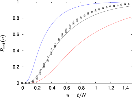
The evolution in well-mixed populations of finite size $N<\infty$ is usually formulated in terms of birth-and-death processes, see, e.g., [154], describing agents formally interacting on a complete graph. The pairwise interactions between a finite number of discrete individuals lead to fluctuations that alter the mean-field predictions. In particular, the Markov chains associated with the CLVM and MLM admit absorbing states and these are unavoidably reached causing the extinction of all but one species, with the surviving species that takes over and ‘fixates’ the entire population. Hence, the above deterministic scenarios (a) and (b) are dramatically modified by demographic fluctuations since the dynamics in a finite population always leads to the survival of one species and the extinction of the two others [108, 109, 71, 110]. Questions of great importance, that have been studied in detail, concern the survival or fixation probability. The former refers to the probability that, starting from a certain initial population composition, a given species survives after an infinitely long time. In the presence of absorbing states in the CLVM and MLM, the only surviving species fixates the population. A related question of great interest is the (unconditional) mean extinction time which is the average time that is necessary for two of the species to go extinct while the third survives (and fixates the population). The question of survival probability is particularly interesting when the species have different reaction rates: For the CLVM with asymmetric rates, when $N$ is large but finite, it has been shown that the species with the smallest dominance rate (the “weakest species”) is the most likely to fixate the population by helping the predator of its own predator [108, 127], a phenomenon referred to as the ‘law of the weakest’. A similar phenomenon has also been found in other three-species models exhibiting cyclic dominance, see, e.g., Ref. [111] and Ref. [165] where a version of the ‘law of the weakest’ was found in a two-dimensional CLVM with mutation. However, it has also been shown that no law of the weakest holds when the number of species in cyclic competition is more than three [166, 167, 159], see also Sec. 4, and that this law is generally not followed when the rates are subject to external fluctuations [168]. The existence of quantities conserved by the CLVM rate equations has been exploited to compute the mean extinction time, found to scale linearly with the system size [109, 71, 110], and the extinction probability $P_{\rm{ext}}(t)$ giving the probability that, starting at ${\bm{s}}={\bm{s}}^{*}$, two of the three species go extinct after a time $t$ [71, 110, 58, 59], see Figure 11.

Figure 11: Extinction probability $P_{\rm{ext}}(t)$ (starting at ${\bm{s}}^{*}$) in the CLVM with $\zeta_{i}=\zeta$ as a function of the rescaled time $u=t/N$: Symbols are stochastic simulation results for different system sizes ($N=100$: triangles; $N=200$: boxes; $N=500$: circles) and solid blue (dark gray) and red (light gray) lines are analytical upper and lower bounds of $P_{\rm{ext}}(t)$, while the black line is the average of these upper and lower bounds. For details, see Ref. [71] from which this figure is reproduced with permission.

Some other aspects of species extinction in well-mixed three-species models exhibiting cyclic dominance have been considered for instance in Refs. [169, 170], and the quasi-cycles arising in these systems have been studied in Refs. [71, 161]. In particular, the quasi-cyclic behavior around the coexistence fixed point of the three-species cyclic model with mutations of Ref. [161] was investigated by computing the power-spectrum and the mean escape time from the coexistence fixed point. In related models, the authors of Ref. [162] studied the entropy production in the nonequilibrium steady state while in Ref. [164] it is shown that demographic noise slows down the quasi cycles of dominance. In Ref. [159], it is shown that for a class of multi-species zero-sum systems the mean-time for the extinction of one species scales linearly with the population size $N$ when the mean-field dynamics predicts the coexistence of all species (and logarithmically with $N$ otherwise), see also Sec. 4.

3.4 Cyclic three-species competition in structured populations

Most ecosystems are spatially extended and populated by individuals that move and interact locally. It is therefore natural to consider spatially-extended models of populations in cyclic competition. When spatial degrees of freedom are taken into account, the interactions between individuals are limited to their neighborhood and this restriction has far-reaching consequences that have been observed experimentally. In fact, since prey may avoid to encounter their predators, species can coexist over long periods. Furthermore, long-term species coexistence is often accompanied by the formation of spatio-temporal patterns such as propagating fronts or spiral waves, see, e.g., [136, 137, 138, 113, 67, 146, 147, 68], that, for instance, have been experimentally observed for Dictyostelium mounds and in Myxobacteria  [171, 172].

Spatially-extended models in which immobile agents of three species occupy the sites of a lattice and interact according to the schemes (18)-(20) have received significant interest, see, e.g., [122, 123, 124, 44, 45, 134, 135, 125, 126, 142]. For instance, the authors of Refs. [44, 45] considered the CLVM with immobile individuals (i.e., with $\zeta>0$ and $\sigma=\beta=\mu=\delta_{D/E}=0$) and showed that spatial inhomogeneities develop on a one-dimensional lattice: A coarsening phenomenon occurs with the formation of a mosaic of single-species domains with algebraically growing size. Spatial degrees of freedom also allow us to consider elementary processes associated with species’ movement such as (22) and (23). This is particularly important in biology where migration has been found to have a profound impact on the maintenance of biodiversity, see, e.g., Refs [120, 121]. In the last two decades, much effort has been dedicated to investigating various aspects of spatially-extended models combining reactions like (18)-(21) and individual’s movement typically modeled by (22) and/or (23). In this context, important issues, both from theoretical and biological perspectives, are:

1. What is the influence of mobility on the survival/coexistence of the species?

2. Is the well-mixed scenario recovered when the individuals are highly mobile?

3. How does mobility affect the spatio-temporal organization of the population?

These questions have been addressed with many variants of the RPS-like systems (18)-(23), and in particular in the framework of the MLM and CLVM. Some of the main findings are reviewed below.

A spatially-extended version of population dynamics with RPS-like interactions is generally formulated at an individual-based level on a regular lattice, most often in two dimensions, which is the natural biologically-relevant choice for the interaction network. In such a setting, a spatially-extended RPS-like model is defined by the processes (18)-(23) implemented on the appropriate lattice (grid or array of patches of finite/infinite carrying capacity). The model’s dynamics is thus formally described by the underlying master equation that appears to be intractable on the face of it. Yet, when fluctuations can be neglected and the linear size $L$ of the lattice is large, the spatial population dynamics of RPS-like systems on a square domain can often be well described in the continuum limit ($L\to\infty$) by the following set of partial differential equations for the local densities $s_{i}\equiv s_{i}({\bm{x}},t)$:

$$\partial_{t}s_{i} = D_{E}\Delta s_{i}+(D_{E}-D_{D})(\rho\Delta s_{i}-s_{i}\Delta\rho)$$ (30)

$$+ s_{i}[\beta(1-\rho)-\sigma s_{i-1}]+\zeta s_{i}[s_{i+1}-s_{i-1}]$$

$$+ \mu\left[s_{i-1}+s_{i+1}-2s_{i}\right],$$

with periodic boundary conditions. Here, the density $s_{i}\equiv s_{i}({\bm{x}},t)$ of species $S_{i}$ is a continuous variable, with $\rho=s_{1}+s_{2}+s_{3}$ and position vector ${\bm{x}}=(x_{1},\dots,x_{d})$. The $d-$dimensional Laplacian is $\Delta=\sum_{i=1}^{d}\partial_{x_{i}}^{2}$. As in most studies we focus on the two-dimensional case, $d=2$, but see also Sec. 3.4.3. The diffusion coefficients $D_{E/D}$ in (30) and the migration rates $\delta_{E/D}$ of (22), (23) are simply related by $D_{E/D}=\delta_{E/D}/L^{2}$. In the first line on the right-hand-side of (30), we recognize the diffusion terms while the second and third lines respectively correspond to the processes of cyclic dominance (18),(19) and mutation (21). It is worth noting that non-linear diffusive terms arise when the pair-exchange and hopping processes (22), (23) are divorced and $\delta_{E}\neq\delta_{D}$ [67, 68, 69], whereas regular (linear) diffusion occurs when any neighboring pairs are exchanged with rate $\delta_{E}=\delta_{D}$ [136, 137, 138, 143, 139, 140, 152]. It is also noteworthy that within the metapopulation formulation of Refs. [67, 145, 68, 148, 69, 70], equations (30) arise at lowest order in an expansion in the inverse of the carrying capacity.

3.4.1 Mobility promotes and jeopardizes biodiversity in models with rock-paper-scissors interactions.

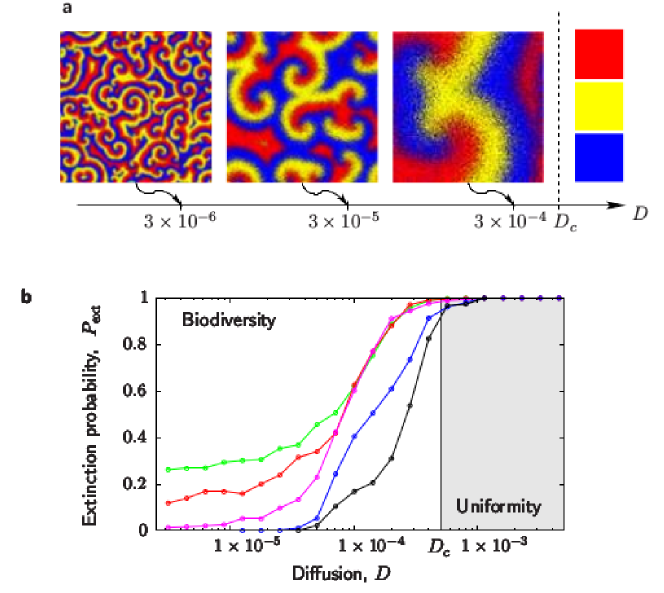
The intriguing role of migration, is well exemplified by a series of in vitro and in vivo experiments: The authors of Refs. [38, 104, 120, 105] showed that when arranged on a Petri dish, three strains of bacteria in cyclic competition coexist for a long time while two species go extinct when the interactions take place in well-shaken flasks. On the other hand, in Ref. [121] it was shown that mobility allows the bacterial colonies in the intestines of co-caged mice to migrate between mice which help maintain the coexistence of bacterial species. Theoretical aspects related to the above questions have been addressed in a series of works [136, 137, 138] on the two-dimensional MLM with at most one individual per lattice site (i.e. $N_{S_{i}}({\bm{\ell}})=0$ or $1$) and symmetric rates, i.e., defined by (18)-(23) with $(\sigma_{i},\zeta_{i},\beta_{i},\mu_{i},\delta_{E},\delta_{D})=(\sigma,0,\beta,0,\delta,\delta)$, that have demonstrated the critical impact of mobility (or migration) on biodiversity. In fact, by considering the above spatially-extended model defined with only dominance-removal, no mutation and exchange between any pairs of neighbors, it was shown that below a critical mobility threshold $D_{c}$ all species coexist in a long-lived quasi-stationary state and form spiraling patterns, whereas biodiversity is lost above the mobility threshold with only one surviving species [136, 137, 138]. This phenomenon was analyzed by combining lattice simulations, with a description in terms of stochastic partial differential equations and a complex Ginzburg–Landau equation [174] derived from equations (30) by approximating heteroclinic orbits with limit cycles. By exploiting the properties of the complex Ginzburg–Landau equation, it has been shown that the extinction probability in the MLM is $P_{{\rm ext}}(t)\approx 0$ at $t=L^{2}\gg 1$ when $D=\delta/L^{2}<D_{c}$. In this case all species coexist and form spiral waves, whereas only one species survives when $D>D_{c}$ and $P_{{\rm ext}}(t=L^{2})\approx 1$, see Fig. 12. Upon estimating the wavelength $\lambda$ of the spiraling patterns, the critical diffusion coefficient $D_{c}$ and the diagram allowing to identify the species coexistence phase were obtained [136, 137, 138]. A similar analysis was then extended to the case of cyclic dominance-removal and dominance-replacement with linear mobility and no mutations, i.e., for the scheme (18)-(23) with rates $(\sigma_{i},\zeta_{i},\beta_{i},\mu_{i},\delta_{D},\delta_{E})=(\sigma,\zeta,\beta,0,\delta,\delta)$ [143, 147].

The experimental findings of Refs. [104, 121] and theoretical results of Refs. [136, 137, 138] suggest that mobility can both promote and jeopardize biodiversity in systems with RPS interactions. Interestingly, recent experiments and agent-based simulations of the range expansion of the E.coli communities used in Ref. [104] showed that cyclic competition alone is not sufficient to guarantee species coexistence in a two-dimensional expanding population: In this case, coexistence depends strongly on the diffusion of the toxin, the composition of the inoculum, and the relative strain growth rates [119].

The oscillatory dynamics characterizing the metastable quasi-stationary state of the two-dimensional MLM has also been studied by computing the species density correlation functions and the Fourier transform of the densities [136, 137, 138, 113]. In Ref. [113], it was shown that for the two-dimensional MLM the above results are robust against quenched disorder in either the reaction rates or mobility rates. Furthermore, the mean extinction time $T_{\rm ex}$ (as the mean time for the first species to go extinct) in the two-dimensional MLM with linear diffusion ($\delta_{D}=\delta_{E}=\delta$) was found to grow exponentially with the lattice size, i.e., $\ln{(T_{\rm ex})}\sim L$, when $D<D_{c}$, whereas $T_{\rm ex}\sim L^{2}$ when $D>D_{c}$ [113]. Further properties of the spiral waves characterizing the species coexistence in the MLM have been investigated. For instance, it has been shown that in the two-dimensional MLM (with $\delta_{D}=\delta_{E}$) a pacemaker (localized periodic input of the three species) is able to maintain target waves that spread across the entire population [140] (see also Ref. [141]). For the same two-dimensional MLM, it has also been found that when the rate of cyclic dominance $\sigma$ exceeds a critical value (the other rates being kept fixed) the spiral waves become unstable Ref. [151] (see also Refs. [68, 69] and Sec. 3.4.2).

Figure 12: The diffusion coefficient $D$ in the two-dimensional MLM with rates $\sigma=\beta=1,\zeta=\mu=0$ and $\delta_{D}=\delta_{C}=\delta$. $D_{c}$ is the critical value, see text. Initially, individuals are randomly distributed. a, Snapshots from lattice simulations of typical states of the system after long temporal development ($t\sim L^{2}$) and for different values of $D$ (each color represents one species, black dots indicate empty spots). Increasing $D$ (from left to right), the spiraling patterns grow, and outgrow the system size when the diffusion coefficient exceeds $D_{c}$: biodiversity is lost above $D_{c}$, see text. b, The extinction probability $P_{\rm ext}$ from stochastic simulations after a waiting time $t=L^{2}$ as function of the diffusion $D$, computed for different system sizes: $N=20\times 20$ (green), $N=30\times 30$ (red), $N=40\times 40$ (purple), $N=100\times 100$ (blue), and $N=200\times 200$ (black), from top to bottom (left side of the figure). Adapted from Ref. [136]

The spatially-extended CLVM with mobile individuals and reaction rates $(\sigma_{i},\zeta_{i},\beta_{i},\mu_{i})=(0,\zeta,0,0)$ has also been extensively studied, both in the case of linear diffusion ($\delta_{D}=\delta_{E}$) and non-linear mobility ($\delta_{D}>0,\delta_{E}=0$), and while all species were still found to coexist in a long-lived quasi-stationary state, they do not form coherent patterns, see, e.g.,[139, 112]. In particular, no spiraling patterns have been observed in the CLVM at either high or low mobility rate: By means of an approximate mapping onto a complex Ginzburg-Landau equation, it has been argued that CLVM cannot sustain spiral waves, which is in stark contrast with the properties of the MLM [139]. Yet, the effect of the range of the cyclic dominance and migration on the dynamics of the two-dimensional CLVM was investigated in Ref. [128], where spatio-temporal patterns (spiral and plane waves) were found in regimes characterized by interactions of sufficiently large range (see also Ref. [133]). The oscillatory dynamics in the metastable coexistence state of the two-dimensional CLVM was studied by computing the time-dependent densities, their Fourier transform and the two-point correlation functions, with results that were found to be robust against quenched disorder in the reaction rates and in the presence/absence of site restriction [112]. In that work, the mean extinction time in the spatial CVLM was found to grow exponentially with the system size in two dimensions, i.e., $\ln{T_{\rm ex}}\sim L$. For extreme choices of the reaction rates, where one species pair reacts much faster than the other two pairs, such that the system is effectively set in one ‘corner’ of parameter space, it has been demonstrated that the resulting stochastic dynamics reduces to the two-species Lotka–Volterra predator-prey model [173].

In Ref. [143], it was found that a two-dimensional model combining dominance-removal and dominance-replacement with linear diffusion (and site restriction) can lead to stable spiraling patterns, as well as to convectively and absolutely unstable spiral waves. This picture was complemented and unified in Refs. [67, 68, 148, 69], as reviewed below.

3.4.2 Spiraling patterns and the complex Ginzburg–Landau equation.

The two-dimensional versions of the generic model (18)-(23) are often characterized by the emergence of long-lived spiraling patterns that can rotate clockwise or anticlockwise whose vortices can be considered as particles that can be annihilated and created in pairs, see Figs. 12 and 13. A satisfactory description of these coherent structures can be obtained in terms of equations (30) and from the complex Ginzburg–Landau equation associated to them. The latter is naturally derived within the metapopulation formulation of Refs. [67, 145, 68, 148, 69, 70] consisting of an array of $L\times L$ patches each of which comprises a well-mixed sub-population of constant size $N$. The composition of each patch changes according to the reactions (18)-(21) and individuals can migrate between two neighboring patches ${\bm{\ell}}$ and ${\bm{\ell}}^{\prime}$ according to the processes (22)-(23). Furthermore, when mutations occur with a rate $\mu>0$, there are no absorbing states and the coexistence state ${\bm{s}}^{*}$ is no longer metastable but a proper reactive steady state. The partial differential equations (30) are obtained at lowest order of a continuum limit $1/N$-expansion of the master equation [154, 57, 155, 60], while a Fokker-Planck equation can be obtained to next order [175, 85, 68].

Figure 13: Top: Phase diagram of the two–dimensional RPS system around the Hopf bifurcation with contours of $c=(c_{{\rm AI}},c_{{\rm EI}},c_{{\rm BS}})$ in the $\sigma-\zeta$ plane, see text. We distinguish four phases: spiral waves are unstable in AI, EI and SA phases, while they are stable in BS phase. The boundaries between the phases have been obtained using the parameter $c$ given by equation (32). Adapted from Ref. [68]. Bottom: Typical long-time snapshots in the AI (left), EI (middle) and BS (right) phases from stochastic simulations of the metapopulation model (18)-(23) at low mutation rate, see text. Each color represents one species (dark dots are regions of low density). The parameters are $L=128$, $N=64$, $(\beta,\sigma,\mu,\delta_{D},\delta_{E})=(1,1,0.001,1,1)$, and $\zeta=1.8$ (left), $1.2$ (middle), and $\zeta=0.6$ (right). In all panels, the initial condition is a random perturbation of $\bm{s}^{*}$. Adapted from Ref. [70].

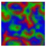
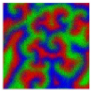
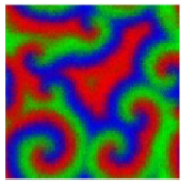
The comparison with stochastic simulations have shown that equations (30) accurately capture the properties of the lattice metapopulation model when $N\gtrsim 20$ [67, 68, 148, 69]. Moreover, the system of partial differential equations (30) can be well approximated by a complex Ginzburg Landau equation [174] derived by performing a multiscale expansion about the ensuing Hopf bifurcation [67, 68, 69]. Such an expansion is performed in terms of the ‘slow’ variables $({\bm{X}},T)=(\epsilon{\bm{x}},~{}\epsilon^{2}t)$, where $\epsilon=\sqrt{3(\mu_{H}-\mu)}$ is the small parameter [176]. The model’s complex Ginzburg Landau equation for the modulated amplitude $\mathcal{A}({\bm{X}},T)$, which is a linear combination of the rescaled species densities [67, 68, 148], thus reads:

$$\partial_{T}\mathcal{A}=D\Delta_{\bm{X}}\mathcal{A}+\mathcal{A}-(1+ic)|\mathcal{A}|^{2}\mathcal{A},$$ (31)

where $\Delta_{\bm{X}}=\partial_{X_{1}}^{2}+\partial_{X_{2}}^{2}=\epsilon^{-2}(\partial_{x_{1}}^{2}+\partial_{x_{2}}^{2})$ and $\partial_{T}=\epsilon^{-2}\partial_{t}$, and after having rescaled $\mathcal{A}$ by a constant, the parameters are

$$c=\frac{12\zeta(6\beta-\sigma)(\sigma+\zeta)+\sigma^{2}(24\beta-\sigma)}{3\sqrt{3}\sigma(6\beta+\sigma)(\sigma+2\zeta)}\quad\text{and}\quad D=\frac{3\beta D_{E}+\sigma D_{D}}{3\beta+\sigma}$$ (32)

equation (31) is thus a controlled approximation of the partial differential equations (30) about the Hopf bifurcation that, in turn, provides a reliable description of the metapopulation stochastic model when $N\gg 1$. The complex Ginzburg Landau equation (31) thus allows us to accurately characterize the spatio-temporal spiraling patterns when $\epsilon\ll 1$ (i.e., $\mu\lesssim\mu_{H}$) and $N\gg 1$ by using the phase diagram of the two-dimensional complex Ginzburg Landau equation, see, e.g., [174]. While this approach is valid when $\epsilon\ll 1$, it also provides significant insight into the system’s spatio–temporal properties away from the Hopf bifurcation (when $\mu\ll\mu_{H}$) [67, 68, 148, 69]:

• For $\mu\lesssim\mu_{H}$ (close to Hopf bifurcation) [67, 68, 148]: Migration yields linear diffusion, which does not alter the stability of the patterns, but $D\to\alpha D\;(\alpha>0)$ only rescales the space and the spiral wavelength as $\lambda\to\lambda/\sqrt{\alpha}$. As shown in the diagram of Figure 13 (top), there are four phases separated by the three critical values $(c_{{\rm AI}},c_{{\rm EI}},c_{{\rm BS}})\approx(1.75,1.25,0.845)$, see Movies at [145]: No spiral waves can be sustained in the ‘absolute instability (AI) phase’ ($c>c_{{\rm AI}}\approx 1.75$); spiral waves are convectively unstable in the Eckhaus instability (EI) phase with $c_{{\rm EI}}\approx 1.25<c<c_{{\rm AI}}$; stable spiral waves are found in the bound state (BS) phase ($c_{{\rm BS}}\approx 0.845<c<c_{{\rm EI}}$); while the vortices corresponding to spiral waves rotating clockwise and anticlockwise can be considered as particles and antiparticles that annihilate in pairs when they collide in the spiral annihilation (SA) phase when $0<c<c_{{\rm BS}}$.

• For $\mu\ll\mu_{H}$ (far from Hopf bifurcation) [68, 148, 70, 152]: Away from the Hopf bifurcation, the AI, EI and BS phases are still present and their boundaries appear to be essentially the same as in the vicinity of the bifurcation [68, 69, 70]. However, at low mutation rate, there is no spiral annihilation and the SA phase is replaced by an extended BS phase, see Fig. 13 (bottom) with far-field breakup of the spiral waves when $\sigma\gg\zeta$ [151, 68]. This analysis confirms that the dynamics does not sustain stable spiral waves when $\zeta\gg\sigma$, and hence corroborates the fact no stable spiraling patterns have been found in the two-dimensional CLVM (with $\zeta>0$ and $\sigma=\mu=0$) [139, 112]. When $\mu\ll\mu_{H}$, non-linear diffusion matters and affects the stability of the spiral waves. In particular, it was shown that when the hopping rate is increased with all the other rates kept constant, a far-field breakup of the spirals occurs when $\delta_{D}\gg\delta_{E}$ [67, 68, 69].

The complex Ginzburg Landau equation (31) permits an accurate prediction of the wavelength $\lambda$ of the spiraling patterns in the BS and EI phases near the Hopf bifurcation where $\mu\lesssim\mu_{H}$ ($\epsilon\ll 1$) [67, 68, 69, 70], and to infer an estimate of the wavelength when $\mu<\mu_{H}$ ($\epsilon={\cal O}(1)$). It has indeed been shown that $\lambda$ decreases linearly with the mutation rate when $\mu<\mu_{H}$ is lowered [68, 70]. Knowing the functional dependence of $\lambda$, it has been possible to unravel the resolution issues arising when the patterns predicted by equations (30) are compared with those found in two-dimensional lattice simulations. This is achieved by determining the range of the diffusion coefficient within which the wavelength of the ensuing patterns is neither too small (of the order of the lattice-space) nor too large (outfitting the domain) for spiral arms to be observable in stochastic simulations on a finite grid [70]. In Ref. [152], the characterization and stability of the spiraling patterns arising in the model (18)-(20) with linear diffusion and no mutations ($\mu=0$) have been obtained directly from equations (30) with linear diffusion ($D_{D}=D_{E}$). Furthermore, the ‘bosonic’ formulation of the MLM (with $S_{i}+S_{i}\to S_{i}$ reactions, see Secs. 2.4 and 2.5) has been considered in Ref. [150] where a noisy complex Ginzburg–Landau equation that accounts for weak fluctuations near the Hopf bifurcation has been derived within the Doi–Peliti path integral formalism. With intrinsic reaction noise thus properly taken into account, the mapping to an effectively two-variable stochastic system is however only valid in a rather restricted range of parameter space; in general three dynamical degrees of freedom are required.

3.4.3 The dynamics of cyclic dominance in one dimension and on complex networks.

The discussion in this section has so far focused on the biologically relevant case of two-dimensional systems. However, the analysis can, at least in principle, be readily extended to one and three dimensions where we would respectively expect traveling and scroll waves instead of spiral waves. In particular, the one-dimensional dynamics of the CLVM and MLM with migration has recently attracted significant interest. In Ref. [112], the mean extinction time of the one-dimensional CLVM with hopping and rates $(\sigma_{i},\zeta_{i},\beta_{i},\mu_{i},\delta_{E},\delta_{D})=(0,\zeta/\delta_{D},0,0,0,1)$ was computed and the power-law dependence $T_{\rm ex}\sim L^{2\gamma}$ with $\gamma\approx 1.5-1.8$ was obtained, while the dynamics was found to be characterized by coarsening and the formation of growing domains with a scaling similar to that of Refs. [44, 45]. The influence of the symmetry of the pair-exchange ($\delta_{D}=\delta_{E}$) and reaction rates on the dynamics of the one-dimensional CVLM has been studied in Ref. [129], while the effect of mutations on the coarsening dynamics and reactive steady state of the one-dimensional CLVM (without migration) was investigated in Ref. [130]. Interestingly, particularly rich dynamics has been found for the one-dimensional MLM with pair-exchange, i.e., for rates $(\sigma_{i},\zeta_{i},\beta_{i},\mu_{i},\delta_{E},\delta_{D})=(\sigma,0,\beta,0,\delta,\delta)$: On a one-dimensional array of patches having a very large carrying capacity, extinction was found to occur via coarsening (rapid extinction), or to be driven by heteroclinic orbits, or through the formation of traveling waves [147]. Besides lattice systems, the dynamics of cyclic dominance between three species has also been studied on random and complex networks, which are settings of particular relevance in the context of evolutionary games and behavioral sciences, see, e.g., Refs. [156, 177, 148] for reviews. It would be interesting to investigate whether the theoretical approaches reviewed here, and devised for lattice systems, could help shed further light on the dynamics of RPS-like systems on complex random topologies, such as small-world networks on which intriguing oscillating patterns have been found [178].

4 Multiple species competition networks

As discussed in the previous section, the many studies of the different variants of the rock-paper-scissors game [157] have revealed the emergence of intriguing phenomena when adding stochastic effects and spatial dependence to the simple cyclic interaction between three species. However, it is important to note that the cyclic three-species game is a very special situation, where all the species interact with each other in a symmetric way. It is obvious that not many of the lessons learned for this special case will be useful when discussing more complex situations (one exception is the fact that spirals will always form when considering an odd number of species where each species attacks only a single other species; however, in contrast to the three-species game these spirals are not composed of individuals belonging to a single species, due to the fact that neutral species partially mix [179, 180]). This is especially true when aiming at an understanding of realistic ecologies, as these ecologies are endowed with complex interaction networks that cannot be captured fully by only considering symmetric networks. As such it is important to study more complex situations and develop theoretical approaches that allow to comprehend the dynamics of more general networks than the cyclic three-species case, with the aim of obtaining a more complete understanding of biodiversity, correlations, and spatio-temporal patterns [1].

In recent years, an increasing number of papers have focused on these more complex situations, ranging from four and more species with symmetric interactions (see [156] for a review of some early results) to general interaction networks with an arbitrary number of species. Whereas the former situation is now fairly well understood, results for more general cases are still rather scarce.

4.1 Symmetric networks

When discussing symmetric networks of competing species, it is useful to introduce the following notation [179]. Consider a system composed of ${\cal N}$ different species. We call model $({\cal N},r)$, $r<{\cal N}$, the model where each of the ${\cal N}$ species preys on $r$ other species. This is done in a cyclic way, i.e., species $i$ preys on species $i+1$, $i+2$, $\cdots$, $i+r$ (this has to be understood modulo ${\cal N}$). $({\cal N},1)$ is therefore identical to the cyclic ${\cal N}$-species game where every species preys on a single species and at the same time is the prey of a different unique predator. On the opposite end $({\cal N},{\cal N}+1)$ describes the situation where every species attacks every other species. Figure 14 shows for illustration the different symmetric predation schemes that are possible for the simple case of four species.

Figure 14: The possible symmetric reaction schemes for a system with four species. The label $({\cal N},r)$ indicates the number of species ${\cal N}$ and the number of prey $r$ for every species.

4.1.1 The cyclic case with one prey and one predator

Already the earliest studies of cyclic cases with four or more species, where every species is preying on one other species while being at the same time the prey of another species, pointed to new effects emerging when going beyond the simple three-species situation. Frachebourg and co-workers considered cyclic Lotka–Volterra systems, where immobile individuals belonging to ${\cal N}$ species interact in a cyclic way [44, 45, 125]. The coarsening taking place in that situation yields the segregation into single-species domains. At a critical number ${\cal N}_{c}$ of species fixation sets in, yielding a frozen state composed of neighboring domains with non-interacting species. This critical number is dependent on the dimensionality of the system, with ${\cal N}_{c}$ increasing from 5 in one space dimension to 23 for the three-dimensional lattice. Another early observation concerns the marked differences between situations with an even or odd number of species [181, 182]. This parity law has a huge impact on the properties of a system, yielding specific space-time patterns and extinction scenarios when the number of species is even.

In a study of the four-species cyclic game on a square lattice, Szabó and Sznaider [183] observed the formation of a defensive alliance where individuals from two non-interacting species (for example, species 1 and 3 for the case (4,1) in figure 14) mix in order to fight off the other alliance. When allowing for mobility of the individuals through jumping to empty neighboring sites, a symmetry breaking ordering is encountered above a critical concentration of empty sites which results in the formation of domains composed by two neutral species. These domains then undergo a coarsening process that stops when one alliance completely fills the lattice. This formation of defensive alliances is a generic property in systems with an even number of species that is very robust to modifications of the model [184, 185, 186].

The cyclic four-species case has been the subject of a series of recent papers [166, 167, 187, 188, 59, 189, 190] that have yielded a rather complete understanding for this case. One emphasis of these studies was on the time evolution of the system and the exploration of the surprisingly rich variety of extinction scenarios. In the well-mixed situation the mean-field rate equations and the correponding deterministic trajectories in configuration space of the population fractions provide a convenient starting point in order to explore not only the end state but also the evolution of the system towards this final state. Inspection of the mean-field equations [166, 167]

$$\partial_{t}a=a\left[k_{A}b-k_{D}d\right]~{}~{};~{}~{}\partial_{t}b=b\left[k_{B}c-k_{A}a\right]$$

$$\partial_{t}c=c\left[k_{C}d-k_{B}b\right]~{}~{};~{}~{}\partial_{t}d=d\left[k_{D}a-k_{C}c\right]$$ (33)

where $a$ denotes the average population fraction of species $A$ and $k_{A}$ the rate at which species $A$ attacks species $B$, reveals that the final state of the system (coexistence or survival of one of the alliances) is completely determined by the key control parameter $\lambda=k_{A}k_{C}-k_{B}k_{D}$. Indeed the quantity

$$Q=\frac{a^{k_{B}+k_{C}}c^{k_{D}+k_{A}}}{b^{k_{C}+k_{D}}d^{k_{A}+k_{B}}}$$ (34)

evolves in the extremely simple manner $Q(t)=Q(0)e^{\lambda t}$. For $\lambda=0$, $Q$ becomes an invariant, and neither pair goes extinct. The system evolves along periodic, closed loops in configuration space that resemble the rim of a saddle, see figure 15a. If, on the other hand, $k_{A}k_{C}\neq k_{B}k_{D}$, then $Q$ decays or grows exponentially, which means that either $bd$ or $ac$ vanishes in the large time limit. Typically, the trajectory in configuration space will be a rather complicated open orbit that spirals toward an absorbing state, see figure 15b for an example. One can also find limiting cases where the trajectory is a straight line that connects the initial state with the final, absorbing state.

Figure 15: (Left) Example of a closed loop (solid curve) in the tetrahedron forming the configuration space for the four species cyclic game, encircling the line of fixed points (green dashed line). (Right) Typical orbit for $\lambda>0$ that starts at the solid green circle and spirals towards an absorbing state, indicated by the red cross on the a-c edge.

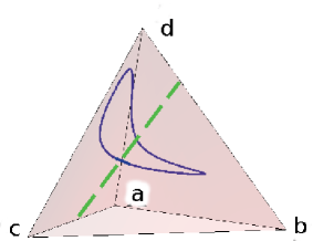
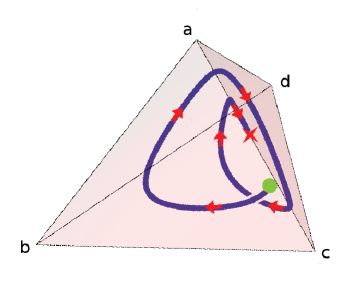
Many of these mean-field features survive when considering the stochastic evolution of finite populations [166, 187]: the stochastic evolution is found to closely follow the mean-field trajectory, with notable deviations only appearing in the vicinity of extinction events. For $\lambda$ close to 0, stochastic effects get more and more important, yielding an increased probability that the system does not end up in the stationary state predicted by mean-field theory. The probability distribution of the domination time $\tau$ [189], i.e., the time needed for one alliance to fill the system, shows for $\lambda=0$ an exponential tail that is a consequence of the fact that the system essentially performs an unbiased random walk in configuration space. The extinction of two species forming an alliance can be viewed as a Poisson process described by an exponential distribution.

Stochastic effects play a very important role when studying the cyclic four-species game on a lattice [188, 189, 190]. For example, the domination time probability distribution reveals the presence of different routes to extinction [189]. In the presence of neutral swappings this probability distribution exhibits for $\lambda=0$ a crossover between two different exponential decays. The earlier regime corresponds to extinctions taking place at very early stages of the coarsening process where small domains contain mainly a single species. The second regime is characterized by very broad tails. These tails result from very rare extinctions of one of the alliances in extremely long-lived states that are due to a stalemate between domains where members of one alliance are well mixed. This transition is encountered in one- and two-dimensional lattices as well as in systems with a fractal dimension.

As already mentioned, mobile individuals in two dimensions may yield a coarsening process where each domain only contains individuals of one alliance. This is of course reminiscent of the well-studied coarsening process taking place in the two-dimensional Ising model when quenching a system prepared in a disordered initial state to temperatures below the critical point [97]. Indeed, when viewing all individuals within one alliance as belonging to the same ‘type’, we end up with two two kinds of domains, in complete analogy to the domains in the Ising model that are formed by a majority of up or down spins. This of course neglects the motion of individuals within domains as well as the preying events that take place at the interface between two domains. In addition, the Ising model is governed by an energy term that via the Boltzmann factor determines the probability to go from one configuration to the next, whereas the four-species model is a non-equilibrium model that breaks detailed balance. As shown in [188], in both models time-dependent quantities do display the same asymptotic behavior. For example, the correlation length $L$ extracted from the space-time correlation displays as asymptotic growth regime a square-root growth $L(t)\sim t^{1/2}$ similar to the Ising model. Interface fluctuations, which can be measured by setting up a system composed of two halves separated by a straight line, with each of the halves containing only individuals from one of the alliances, undergo a roughening process characterized by the same roughening exponents as an Ising interface.

Some variations of the basic scheme with four species that have also been studied include situations where the predation rate is not the same for all species [186] or is spatially variable [190] as well as cases where an individual changes its character following a time-dependent probability distribution [191].

Many of the results obtained for this simple cyclic four-species case with one prey and one predator remain valid when considering a larger even number of species with the same interaction scheme [185, 167, 192]. In all cases, two alliances, each composed of half of the species, are competing against each other, yielding similar phenomena as for the four-species case, especially when all the predation rates are the same. As shown in [167], at the mean-field level all the conclusions reached for the four-species game with arbitrary values of the rates are recovered when considering a larger even number of species.

4.1.2 Other symmetric interaction networks

A straightforward way to generalize the simple cyclic case with a unique prey for each species is to consider instead $r>1$ prey which yields the already mentioned $({\cal N},r)$ models when done in a cyclic way [179, 193, 194]. Increasing the number of prey yields a rich variety of different space-time patterns as illustrated in figure 16 for the six-species case. Whereas for (6,1) two teams composed each of three non-interacting species yield the already described coarsening process with two types of domains, the (6,2) model results in a coarsening process with three different types of domains, each domain being formed by two mutually neutral species, see figure 16a. The case (6,3) shown in figure 16b is a very interesting one: within each of the two types of domains three species undergo a cyclic rock-paper-scissors game [195]. The (6,4) game in figure 16c is characterized by spirals and propagating wave fronts. Finally, for (6,5) every species attacks every other species which results in segregation and the formation of coarsening clusters that only contain individuals from one species, see figure 16d.

(a)                                   (b)

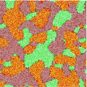
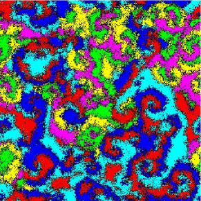
(c)                                   (d)

Figure 16: (Color online) Space-time patterns emerging when changing the number of prey in the case of six species: (a) coarsening of three different types of domains for (6,2), (b) two coarsening domain types with a non-trivial rock-paper-scissors game within the domains for (6,3), (c) spirals and propagating wave fronts for (6,4), (d) segregation and formation of pure domains for (6,5). All rates have been chosen equal to 1. For (a) different colors than for the other three cases were chosen for clarity.

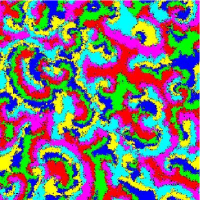
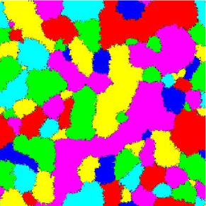
These patterns can be predicted by considering the square $\underline{B}=\underline{A}^{2}$ of the adjacancy matrix $\underline{A}$ [179]. This matrix $\underline{B}$ contains information about preferred partnership formation. Indeed, when representing the game by a directed graph like those shown in figure 14, element $b_{ij}$ then counts the number of paths of length 2 from vertex $i$ to vertex $j$, i.e., paths of the form $i\longrightarrow k\longrightarrow j$ where $k$ is not equal to $i$ or $j$. Following the maxim that the enemy of my enemy is my friend, species $j$ then has a preference to ally with the species that preys on most of its predators, this preferred ally of $j$ being identified by the condition $\max_{i}b_{ij}$. Whereas analysis of $\underline{B}$ is enough to fully characterize $({\cal N},r)$ games with identical rates for all predation events, it can fail in the classification of extinction scenarios when rates are not identical. In these situations the analysis of the Pfaffian of the interaction matrix has been shown to yield insights into the conditions for coexistence [159].

It is remarkable that some of the space-time patterns are characterized by a coarsening process with a non-trivial dynamics inside the domains. One example can be found in figure 16b which shows that for the (6,3) system a rock-paper-scissors game between the three species of a team is sustained. This emergence of spirals within coarsening dynamics give rise to non-trivial internal dynamics. This non-trivial dynamics inside the domains affects the coarsening process as well as the properties of the interfaces separating different domains, yielding sets of exponents that differ markedly from those usually encountered in systems with curvature driven coarsening [195]. Whereas this appearance of spirals within coarsening domains has originally been found for the case with site restriction where a site is occupied by at most one individual [179], this intriguing space-time pattern is also observed in a “bosonic” implementation without a hard constraint on the occupation number per site [149].

The papers [196, 197] discuss the spatial (6,2) game in presence of predation rates that are not homogeneous. Assuming that species $i$ replaces species $i+1$ with rate $\alpha$ and species $i+2$ with rate $\gamma$, the increase of mobility yields a transition between a steady state where a three-species cyclic alliance prevails and a steady state where after the end of the coarsening process shown in figure 16a one of the two-species neutral alliances fill the system. If $\gamma\neq\alpha$, then the three neutral alliances do not undergo the coarsening process shown in figure 16a, but instead they play a spatial rock-paper-scissors game [197]. This behavior is not predicted by the analysis of the square of the adjacency matrix, thus highlighting that for non-homogeneous rates the approach of [179] does not allow to reliably predict the fate of an ecology. Introducing one more parameter by allowing for alliance-specific heterogeneous predation rates, an even more complex behavior is observed, resulting in a non-monotonic dependence of alliance survival on the difference of alliance-specific predation rates [196].

A broader class of May–Leonard type systems that contains the $({\cal N},r)$ models as special cases has been studied by Avelino and co-workers in a series of papers [198, 199, 200, 201, 202]. Labeling the ${\cal N}$ different species by $i$ and making the cyclic identification $i=i+k{\cal N}$, with $k$ an integer, these authors consider both right- and left-handed predation where a species $i$ attacks up to $\alpha_{R}$ species to their right along the cycle and up to $\alpha_{L}$ species to their left along the cycle. $({\cal N},r)$ models are obtained when $\alpha_{R}=r$ and $\alpha_{L}=0$. In their analysis Avelino et al. focus on the emerging (interface) string network of empty sites and the corresponding junctions between these strings. Depending on the number of species and the chosen interactions, different types of junctions, associated to regions with a high concentration of empty sites, are identified.

A spatial five-species game with two prey and two predators, where species $i$ replaces species $i+1$ with rate $p_{1}$ and species $i-2$ with rate $p_{2}$, was the topic of some recent papers [203, 204, 205]. This model is an analogy of the rock-paper-scissors-lizard-Spock game. Interestingly, this model presents a special ratio of the two rates (coined the golden point rule in [203]) $q=p_{1}/p_{2}=\frac{\sqrt{5}-1}{2}$ where two of the five eigenvalues of the interaction matrix vanish. This results in a zero-frequency mode whose presence yields a vanishing dominance between any pair of mean-field solutions. Monte Carlo simulations on the two-dimensional lattice show that this dominance vanishing also holds beyond the mean-field approximation and yields a divergence of the species density fluctuations [204]. Interesting results have also been obtained for the ratio $q=1$ where one encounters the emergence of various local groups of three species each in different spatial regions [205]. Changing the mobility results in transitions between different steady states.

4.2 General competition and food networks

An increasing, albeit still small, number of recent papers have focused on non-symmetric interaction networks. One of the dominant research thrust in this context is the question how biodiversity and extinction scenarios change when going from a fully cyclic (non-transitive) situation to a hierarchical (transitive) network by adding or modifying directed links. Examples include three-species cycles where one link is reversed [206], four-species cycles where three species are engaged in cyclic competition, whereas the fourth species interacts with the other three in various ways [207, 208, 209, 206], a five-species cycle with additional links that yields five different levels of hierarchy [210], six-species games where the condition of two prey and two predators is imposed in various ways (the symmetric version being the (6,2) game) [211, 212], as well as nine-species cycles with complex interactions supposed to mimic the biochemical war among bacteria capable of producing at most two different toxins [213, 214].

Whereas these different studies point to the amazingly rich properties of non-symmetric games, it is difficult to draw general conclusions from specific case studies. As already mentioned, it was proposed in [159] to use the Pfaffian of the interaction matrix in order to understand the conditions for biodiversity of complex systems. This has been successfully applied to a transitive four-species game as well as to a five-species cycle with heterogeneous predation rates. However, no systematic studies beyond these specific cases have been published. An interesting path for further progress is provided by Szabó et al [215] who show that cyclic dominance of ${\cal N}$ species can be decomposed into $\left({\cal N}-1\right)\left({\cal N}-2\right)/2$ RPS-type independent components.

In [194] Roman et al. build on the work [179] and propose different matrices, derived from the adjacency matrix, that allow to fully characterize cases where the predation rates are homogeneous. Of course, in real ecologies the condition of homogeneity of predation rates is not fulfilled. Still, restricting oneself to this situation already yields important insights in the properties of general food networks, especially when classifying the possible inter-species relationships. The additional matrices needed for general interaction schemes encompass the alliance matrix whose elements provide information on the best possible ally for each species, the prey-allies and neutral allies matrices that distinguish for each species between allies hunted by that species and allies towards which that species has a neutral approach, as well as one additional matrix that allows to identify neutral intermediaries between different species. As illustrated in [194] these matrices reveal the full inter-species relationships for the most complex predator-prey systems as well as the possible extinction scenarios.

As a final remark we point out that one can also consider time-dependent rates and/or adjacency matrices in order to mimic various perturbations to an ecological system, ranging from seasonal changes to the introduction of new species (for example through migration). In [216] new species are introduced with some probability at empty sites, whereas interactions between the new species and already existing species are formed randomly. In [217] different perturbations are applied to the spatial (6,3) game (one perturbation involves changing the interaction scheme to (6,2) during the coarsening process shown in figure 16b) and their effects are studied through the analysis of various time-dependent quantities. These few studies provide some of the possible starting points for a systematic investigation of the effects perturbations can have on predator-prey systems.

5 Conclusion and outlook

In this topical review, we have focused on stochastic predator-prey population dynamics in spatially extended systems, and the investigation of dynamical correlations and fluctuations beyond the realm of the standard mean-field rate equation analysis, which often turns out inadequate in this context. We have specifically demonstrated how the transfer of both analytical as well as numerical simulation tools from non-equilibrium statistical physics has led to a host of unexpected novel and intriguing phenomena in these simple paradigmatic model systems. These range from persistent population oscillations stabilized by intrinsic demographic reaction noise and strong correlation-induced renormalizations of the associated kinetic parameters to the emergence of genuine continuous out-of-equilibrium phase transitions, as well as the spontaneous formation of remarkably rich spatio-temporal patterns. We have discussed how the availability of spatial degrees of freedom can drastically extend extinction times through the emergence of such noise-stabilized structures, and hence promote ecological stability and species diversity. We have also elucidated how spontaneous pattern formation and coarsening kinetics in multi-species competition networks can be understood and classified on the basis of mean-field theory. Detailed investigations over the past two decades of stochastic spatial predator-prey dynamics have thus enriched our grasp and characterization of strongly out-of-equilibrium systems. As a striking example, let us mention the recently uncovered intimate connection of the directed percolation active-absorbing transition in predator-prey systems with the long-unresolved problem of the onset of turbulence in shear flows [218].

We hope that the fields of ecology, population genetics, and epidemiology will in turn benefit from this much improved theoretical understanding of complex stochastic interacting and reacting particle models. This is of course not limited to the predator-prey type models that are the subject of this overview. Non-equilibrium statistical physics has had a similarly strong impact on the study of stochastic and spatially extended single-’species’ ecological systems; an up-to-date brief review is presented in Ref. [219]. Yet of course the very simplified idealized models studied here cannot possibly capture the full complexity encountered in natural ecosystems. Nevertheless, we believe that the distinct physics approach of first isolating fundamental phenomena and identifying basic quantitative features in reduced paradigmatic models and then re-synthesizing these into much more complicated systems should prove fruitful in ecology and population biology as well. Experimental verification of the relevance of correlation and fluctuation effects in simple artificial ecosystems whose dynamical evolution is fully controllable would naturally constitute a crucial step towards validation of this assertion. We cannot provide an exhaustive list of attempts along this direction here, but merely mention two representative and quite promising recent developments, namely (i) the construction of predator-prey molecular ecosystems in appropriately tailored DNA strands [220]; and (ii) the genetic programming of E. coli bacteria to display various desired ecological features [221]. We trust these and other efforts to construct controlled synthetic ecosystems in the laboratory will turn out fruitful in the near future and provide major novel avenues for both experimental and theoretical research in the area of stochastic spatially extended population dynamics.

References

- [1] May R M 1973 Stability and complexity in model ecosystems (Princeton: Princeton University Press)
- [2] Maynard Smith J 1974 Models in ecology (Cambridge: Cambridge University Press)
- [3] Hofbauer J and Sigmund K 1998 Evolutionary Games and Population Dynamics (Cambridge: Cambridge University Press)
- [4] Murray J D 2002 Mathematical biology vols. I and II (New York: Springer, 3rd ed.)
- [5] Neal D 2004 Introduction to Population Biology (Cambridge: Cambridge University Press)
- [6] Kingsland S E 1985 Modeling Nature (Chicago: The University of Chicago Press)
- [7] Schuster S, Kreft J-U, Schroeter A and Pfeiffer T 2008 Use of game-theoretical methods in biochemistry and biophysics J. Biol. Phys. 34 1
- [8] Hanski I A and Gagiotti O E (eds.) 2004 Ecology, genetics, and evolution of metapopulations (Amsterdam: Elsevier Academic Press)
- [9] Kim M-Y, Roy R, Aron J L, Carr T W and Schwartz I B 2005 Scaling behavior of laser population dynamics with time-delayed coupling: theory and experiment Phys. Rev. Lett. 94 088101
- [10] Malthus T R 1798 An Essay on the Principle of Population (London: J. Johnson)
- [11] Vineis P and Berwick B 2006 The population dynamics of cancer: a Darwinian perspective Int. J. Epidemiol. 35 1151
- [12] Cross M C and Hohenberg P C 1993 Pattern formation outside of equilibrium Rev. Mod. Phys. 65 851
- [13] Cross M and Greenside H 2009 Pattern Formation and Dynamics in Nonequilibrium Systems (Cambridge: Cambridge University Press)
- [14] Verhulst P-F 1838 Notice sur la loi que la population suit dans son accroissement Corr. Math. Phys. 10 110
- [15] Lotka A J 1925 Elements of Physical Biology (Baltimore: Williams and Wilkins)
- [16] Pearl R 1925 The Biology of Population Growth (New York: Alfred A. Knopf)
- [17] Volterra V 1926 Variazioni e fluttuazioni del numero d’individui in specie animali conviventi Mem. Accad. Lincei Roma 2 31; Fluctuations in the abundance of a species considered mathematically Nature (London) 118 558
- [18] Lotka A J 1920 Analytical note on certain rhythmic relations in organic systems Proc. Natl. Acad. Sci. U.S.A. 6 410; Undamped oscillations derived from the law of mass action J. Amer. Chem. Soc. 42 1595
- [19] Gause G F 1934 The Struggle for Existence (Williams and Wilkins, Baltimore)
- [20] Royama T 1971 A comparative study of models for predation and parasitism Res. Popul. Ecol. (Kyoto) 13 1
- [21] Sigmund K 2007 Kolmogorov and population dynamics in Charpentier E, Lesne A and Nikolski N K (eds.) Kolmogorov’s Heritage in Mathematics (Berlin: Springer)
- [22] Kolmogorov A N 1936 Sulla teoria di Volterra della lotta per l’esistenza Giornale Istituto Ila. Attuari 7 74
- [23] McKendrick A G 1926 Applications of mathematics to medical problems Proc. Ed. Math. Soc. 44 98
- [24] Bacaër N 2011 McKendrick and Kermack on epidemic modelling (1926-1927) in A Short History of Mathematical Population Dynamics (London: Springer) pp. 89–96
- [25] MacLulich D A 1937 Fluctuations in the numbers of the varying hare (Lepus americanus) University of Toronto Studies Biological Series 43 (Toronto: The University of Toronto Press)
- [26] Hewitt C G 1921 The Conservation of the Wild Life of Canada (New York: C. Scribner’s Sons)
- [27] Huffaker C B 1958 Experimental studies on predation: dispersion factors and predator-prey oscillations Hilgardia 27 343
- [28] Kimura M 1953 “Stepping stone” model of population Ann. Rept. Nat. Inst. Genetics, Japan 3 62
- [29] Kimura M and Weiss G H 1964 The stepping stone model of population structure and the decrease of genetic correlation with distance Genetics 49 561
- [30] Durrett R 1999 Stochastic spatial models SIAM Review 41 677
- [31] Moran P A P 1958 Random processes in genetics Math. Proc. Camb. Philos. Soc. 54 60
- [32] Nowak M A 2006 Evolutionary Dynamics (Belknap Press, Harvard University Press, Cambridge, MA, U.S.A.)
- [33] Levins R 1969 Some demographic and genetic consequences of environmental heterogeneity for biological control Bull. Entomol. Soc. Am. 15 237
- [34] Hastings A 1977 Spatial heterogeneity and the stability of predator-prey systems Theor. Pop. Biol. 12 37
- [35] Maynard Smith J and Price G R 1973 The logic of animal conflict Nature (London) 246 15
- [36] Maynard Smith J 1982 Evolution and the Theory of Games (Cambridge: Cambridge University Press)
- [37] May R M and Leonard W 1975 Nonlinear aspects of competition between three species SIAM J. Appl. Math. 29 243
- [38] Sinervo B and Lively C M 1996 The rock-paper-scissors game and the evolution of alternative male strategies Nature (London) 380 240
- [39] Kerner E H 1957 A statistical mechanics of interacting biological species Bull. Math. Biophys. 19 121
- [40] Dunbar S 1983 Travelling wave solutions of diffusive Lotka–Volterra equations J. Math. Biol. 17 11
- [41] Matsuda H, Ogita N, Sasaki A and Satō K 1992 Statistical mechanics of population – the lattice Lotka–Volterra model Prog. Theor. Phys. 88 1035
- [42] Satulovsky J E and Tomé T 1994 Stochastic lattice gas model for a predator-prey system Phys. Rev. E 49 5073
- [43] Boccara N, Roblin O and Roger M 1994 Automata network predator-prey model with pursuit and evasion Phys. Rev. E 50 4531
- [44] Frachebourg L, Krapivsky P L and Ben-Naim E 1996 Segregation in a one-dimensional model of interacting species Phys. Rev. Lett. 77 2125
- [45] Frachebourg L, Krapivsky P L and Ben-Naim E 1996 Spatial organization in cyclic Lotka–Volterra systems Phys. Rev. E 54 6186
- [46] Rauch E M, Sayama H and Bar-Yam Y 2003 Dynamics and genealogy of strains in spatially extended host-pathogen models J. Theor. Biol. 221 655
- [47] de Aguiar M A M, Rauch E M and Bar-Yam Y 2003 Mean-field approximation to a spatial host-pathogen model Phys. Rev. E 67 047102
- [48] de Aguiar M A M, Rauch E M and Bar-Yam Y 2004 Invasion and extinction in the mean field approximation for a spatial host-pathogen model J. Stat. Phys. 114 1417
- [49] Haken H 1983 Synergetics (New York: Springer, 3rd ed.)
- [50] Mobilia M, Georgiev I T and Täuber U C 2007 Phase transitions and spatio-temporal fluctuations in stochastic lattice Lotka–Volterra models J. Stat. Phys. 128 447
- [51] Dobramysl U and Täuber U C (2013) Environmental versus demographic variability in stochastic predator-prey models J. Stat. Mech. 2013 P10001
- [52] Täuber U C 2012 Population oscillations in spatial stochastic Lotka–-Volterra models: a field-theoretic perturbational analysis J. Phys. A: Math. Theor. 45 405002
- [53] Sherratt J, Eagen B T and Lewis M A 1997 Oscillations and chaos behind predator-prey invasion: mathematical artifact or ecological reality? Phil. Trans. R. Soc. Lond. B 352 21
- [54] Hosono Y 1998 The minimal speed of traveling fronts for a diffusive Lotka–Volterra competition model Bull. Math. Biol. 60 435
- [55] McKane A J and Newman T J 2005 Predator-prey cycles from resonant amplification of demographic stochasticity Phys. Rev. Lett. 94 218102
- [56] Gillespie D T 1976 A general method for numerically simulating the stochastic time evolution of coupled chemical reactions J. Comput. Phys. 22 403
- [57] Van Kampen N G 1992 Stochastic Processes in Physics and Chemistry (Amsterdam: Elsevier)
- [58] Parker M and Kamenev A 2009 Extinction in the Lotka–Volterra model Phys. Rev. E 80 021129
- [59] Dobrinevski A and Frey E 2012 Extinction in neutrally stable stochastic Lotka–Volterra models Phys. Rev. E 85 051903
- [60] Täuber U C 2014 Critical Dynamics – A Field Theory Approach to equationilibrium and Non-equationilibrium Scaling Behavior (Cambridge: Cambridge University Press)
- [61] Assaf M and Meerson B 2017 WKB theory of large deviations in stochastic populations J. Phys. A: Math. Theor. 50 263001
- [62] Parker M and Kamenev A 2009 Mean extinction time in predator-prey model J. Stat. Phys 141 201
- [63] Dimentberg M F 2002 Lotka–Volterra system in a random environment Phys. Rev. E 65 036204
- [64] Chen S and Täuber U C 2016 Non-equilibrium relaxation in a stochastic lattice Lotka–Volterra model Phys. Biol. 13 025005
- [65] Washenberger M J, Mobilia M and Täuber U C 2007 Influence of local carrying capacity restrictions on stochastic predator-prey models J. Phys. Cond. Matt. 19 065139
- [66] Cao Y, Hong L and Petzold L 2004 Efficient formulation of the stochastic simulation algorithm for chemically reacting systems J. Chem. Phys. 121 4059
- [67] Szczesny B, Mobilia M and Rucklidge A M 2013 When does cyclic dominance lead to stable spiral waves? EPL (Europhys. Lett.) 102 28012
- [68] Szczesny B, Mobilia M and Rucklidge A M 2014 Characterization of spiraling patterns in spatial rock-paper-scissors games Phys. Rev. E 90 032704
- [69] Szczesny B 2014 Coevolutionary dynamics in structured populations of three species PhD Thesis University of Leeds (URL: http://etheses.whiterose.ac.uk/id/eprint/7547)
- [70] Mobilia M, Rucklidge A M and Szczesny B 2016 The influence of mobility rate on spiral waves in spatial rock-paper-scissors games Games 7 24 (published under the CC-BY license, http://creativecommons.org/licenses/by/4.0/)
- [71] Reichenbach T, Mobilia M and Frey E 2006 Coexistence versus extinction in the stochastic cyclic Lotka–Volterra model Phys. Rev. E 74 051907
- [72] Provata A, Nicolis G and Baras F 1999 Oscillatory dynamics in low-dimensional supports: a lattice Lotka–Volterra model J. Chem. Phys. 110 8361
- [73] Rozenfeld A F and Albano E V 1999 Study of a lattice-gas model for a prey-predator system Physica A 266 322
- [74] Lipowski A 1999 Oscillatory behavior in a lattice prey-predator system Phys. Rev. E 60 5179
- [75] Lipowski A and Lipowska D 2000 Nonequilibrium phase transition in a lattice prey-predator system Physica A 276 456
- [76] Monetti R, Rozenfeld A F and Albano E V 2000 Study of interacting particle systems: the transition to the oscillatory behavior of a prey-predator model Physica A 283 52
- [77] Droz M and Pȩkalski A 2001 Coexistence in a predator-prey system Phys. Rev. E 63 051909
- [78] Antal T and Droz M 2001 Phase transitions and oscillations in a lattice prey-predator model Phys. Rev. E 63 056119
- [79] Tsekouras G A and Provata A 2001 Fractal properties of the lattice Lotka–Volterra model Phys. Rev. E 65 016204
- [80] Kowalik M, Lipowski A and Ferreira A L 2002 Oscillations and dynamics in a two-dimensional prey-predator system Phys. Rev. E 66 066107
- [81] Mobilia M, Georgiev I T and Täuber U C 2006 Fluctuations and correlations in lattice models for predator-prey interaction Phys. Rev. E 73 040903
- [82] Dobramysl U and Täuber U C 2008 Spatial variability enhances species fitness in stochastic predator-prey interactions Phys. Rev. Lett. 101 258102
- [83] Dobramysl U and Täuber U C (2013) Environmental versus demographic variability in two-species predator-prey models Phys. Rev. Lett. 110 048105
- [84] Movies of Monte Carlo simulation runs with various parameter settings can be viewed at: http://www.phys.vt.edu/tauber/PredatorPrey/movies/
- [85] Butler T and Goldenfeld N 2009 Robust ecological pattern formation induced by demographic noise Phys. Rev. E 80 030902(R)
- [86] Butler T and Goldenfeld N 2011 Fluctuation-driven Turing patterns Phys. Rev. E 84 011112
- [87] Rozenfeld A F and Albano E V 2001 Critical and oscillatory behavior of a system of smart preys and predators Phys. Rev. E 63 061907
- [88] Rozenfeld A F and Albano E V 2004 A self-organized system of smart preys and predators Phys. Lett. A 332 361
- [89] Täuber U C, Howard M and Vollmayr-Lee B P 2005 Applications of field-theoretic renormalization group methods to reaction-diffusion problems J. Phys. A: Math. Gen. 38 R79
- [90] Cardy J, Gawedzki K and Falkovich G 2008 Non-equilibrium Statistical Mechanics and Turbulence London Mathematical Society Lecture Note Series 355 eds. Nazarenko S and Zaboronski O V (Cambridge: Cambridge University Press)
- [91] Hinrichsen H 2000 Nonequilibrium critical phenomena and phase transitions into absorbing states Adv. Phys. 49 815
- [92] Ódor G 2004 Universality classes in nonequilibrium lattice systems Rev. Mod. Phys. 76 663
- [93] Janssen H K and Täuber U C 2005 The field theory approach to percolation processes Ann. Phys. (NY) 315 147
- [94] Henkel M, Hinrichsen H and Lübeck S 2008 Non-equationilibrium Phase Transitions vol. 1: Absorbing Phase Transitions (Bristol: Springer)
- [95] Janssen H K 2001 Directed percolation with colors and flavors J. Stat. Phys. 103 801
- [96] Cardy J L and Sugar R L 1980 Directed percolation and Reggeon field theory J. Phys. A: Math. Gen. 13 L423
- [97] Henkel M and Pleimling M 2010 Non-equationilibrium Phase Transitions vol. 2: Ageing and Dynamical Scaling Far From equationilibrium (Bristol: Springer)
- [98] Cantrell R S and Cosner C 1991 The effects of spatial heterogeneity in population dynamics J. Math. Biol. 29 315
- [99] Cantrell R S and Cosner C 1998 On the effects of spatial heterogeneity on the persistence of interacting species J. Math. Biol. 37 103
- [100] Heiba B, Chen S and Täuber U C 2018 Boundary effects on population dynamics in stochastic lattice Lotka–Volterra models Physica A 491 582
- [101] Yoshida T, Jones L E, Ellner S P, Fussmann G F and Hairston N G Jr 2003 Rapid evolution drives ecological dynamics in a predator-prey system Nature 424 303
- [102] Yoshida T, Ellner S P, Jones L E, Bohannan B J M, Lenski R E and Hairston Jr N G 2007 Cryptic population dynamics: rapid evolution masks trophic interactions PLoS Biol. 5 e235
- [103] Pennisi E 2005 What determines species diversity? Science 309 90
- [104] Kerr B, Riley M A, Feldman M W and Bohannan B J M 2002 Local dispersal promotes biodiversity in a real-life game of rock-paper-scissors Nature (London) 418 171
- [105] Nahum J R, Harding B N and Kerr B 2011 Evolution of restraint in a structured rock-paper-scissors community Proc. Natl. Acad. Sci. U.S.A. 108 10831
- [106] Sinervo B, Miles D B, Frankino W A, Klukowski M and DeNardo D F 2000 Testosterone, endurance, and Darwinian fitness: Natural and sexual selection on the physiological bases of alternative male behaviors in side-blotched lizards Hormones and Behaviour 38 222
- [107] Jackson J B C and Buss L 1975 Allelopathy and spatial competition among coral reef invertebrates Proc. Nat. Acad. Sci. USA 72 5160
- [108] Frean M and Abraham E D 2001 Rock-scissors-paper and the survival of the weakest Proc. R. Soc. Lond. B 268 1323
- [109] Ifti M and Bergensen B 2003 Survival and extinction in cyclic and neutral three-species systems Eur.Phys. J. E 10 241
- [110] Reichenbach T, Mobilia M and Frey E 2008 Stochastic effects on biodiversity in cyclic coevolutionary dynamics Banach centre Publications 80 259
- [111] Müller A P O and Gallas J A C 2010 How community size affects survival chances in cyclic competition games that microorganisms play Phys. Rev. E 82 052901
- [112] He Q, Mobilia M and Täuber U C 2010 Spatial rock-paper-scissors models with inhomogeneous reaction rates Phys. Rev. E 82 051909
- [113] He Q, Mobilia M and Täuber U C 2011 Coexistence in the two-dimensional May–Leonard model with random rates Eur. Phys. J. B 82 97
- [114] Turing A M 1952 The chemical basis of morphogenesis Phil. Trans. R. Soc. B 237 37
- [115] Koch A J and Meinhardt H 1994 Biological pattern formation: from basic mechanisms to complex structures Rev. Mod. Phys 66 1481
- [116] Levin S A and Segel L A 1976 Hypothesis to explain the origin of planktonic patchness Nature (London) 259, 659
- [117] Hassel M P, Comins H N and May R M 1994 Species coexistence and self-organizing spatial dynamics Nature (London) 370 290
- [118] Maron J L and Harrison S 1997 Spatial pattern formation in an insect host-parasitoid system Science 278 1619
- [119] Weber M F, Poxleitner G, Hebisch E, Frey E, and Opitz M 2014 Chemical warfare and survival strategies in bacterial range expansions J. R. Soc. Interface 11 20140172
- [120] Kerr B, Neuhauser C, Bohannan B J M and Dean A M 2006 Local migration promotes competitive restraint in a host-pathogen tragedy of the commons Nature (London) 442 75
- [121] Kirkup BC and Riley M A 2004 Antibiotic-mediated antagonism leads to a bacterial game of rock-paper-scissors in vivo Nature (London) 428 412
- [122] Tainaka K-I 1988 Lattice model for the Lotka–Volterra system J. Phys. Soc. Jpn 57 2568
- [123] Tainaka K-I 1989 Stationary pattern of vortices or strings in biological systems: lattice version of the Lotka–Volterra model Phys. Rev. Lett. 63 2688
- [124] Tainaka K-I 1994 Vortices and strings in a model ecosystem Phys. Rev. E 50 3401
- [125] Frachebourg L and Krapivsky P L 1998 Fixation in a cyclic Lotka–Volterra model. J. Phys. A 31 L287
- [126] Szabó G and Szolnoki A 2002 Three-state cyclic voter model extended with Potts energy Phys. Rev. E 65 036115
- [127] Berr M, Reichenbach T, Schottenloer M and Frey E 2009 Zero-one survival behavior of cyclically competing species Phys. Rev. Lett. 102 048102
- [128] Ni X, Wang W X, Lai Y C and Grebogi C 2010 Cyclic competition of mobile species on continuous space: Pattern formation and coexistence Phys. Rev. E 82 066211
- [129] Venkat S and Pleimling M 2010 Mobility and asymmetry effects in one-dimensional rock-paper-scissors games Phys. Rev. E 81 021917
- [130] Winkler A A, Reichenbach T and Frey E 2011 Coexistence in a one-dimensional cyclic dominance process Phys. Rev. E 81 060901(R)
- [131] Juul J, Sneppen K and Mathiesen J 2013 Labyrinthine clustering in a spatial rock-paper-scissors ecosystem Phys. Rev. E 87 042702
- [132] Mitarai N, Gunnarson I, Pedersen B N, Rosiek C A and Sneppen K 2016 Three is much more than two in coarsening dynamics of cyclic competitions Phys. Rev. E 93 042408
- [133] Avelino P P, Bazeia D, Losano L, Menezes J and de Oliveira B F 2017 Spiral patterns and biodiversity in lattice-free Lotka-Volterra models e-print: arXiv:1710.05066
- [134] Durrett R and Levin S 1997 Allelopathy in spatially distributed populations J. Theor. Biol. 185 165
- [135] Durrett R and Levin S 1998 Spatial aspects of interspecific competition Theor. Pop. Biol. 53 30
- [136] Reichenbach T, Mobilia M and Frey E 2007 Mobility promotes and jeopardizes biodiversity in rock-paper-scissors games Nature (London) 448 1046
- [137] Reichenbach T, Mobilia M and Frey E 2007 Noise and correlations in a spatial population model with cyclic competititon Phys. Rev. Lett. 99 238105
- [138] Reichenbach T, Mobilia M and Frey E 2008 Self-organization of mobile populations in cyclic competititon J. Theor. Biol. 254 368
- [139] Peltomäki M and Alava M 2008 Three-and four-state rock-paper-scissors games with diffusion Phys. Rev. E 78 031906
- [140] Jiang L-L, Zhou T, Perc M, Huang X and Wang B 2009 Emergence of target waves in paced populations of cyclically competing species New J. Phys. 11 103001
- [141] Wang W-X, Ni X, Lai Y-C and Grebogi C 2011 Pattern formation, synchronization, and outbreak of biodiversity in cyclically competing games Phys. Rev. E 83 011917
- [142] Rulands S, Reichenbach T and Frey E 2011 Threefold way to extinction in populations of cyclically competing species J. Stat. Mech. (2011) L01003
- [143] Reichenbach T and Frey E 2008 Instability of spatial patterns and its ambiguous impact on species diversity Phys. Rev. Lett. 101 058102
- [144] Hanski, I 1999 Metapopulation Ecology (New York: Oxford University Press)
-
[145]
Szczesny B, Mobilia M and Rucklidge A M 2012
Figshare, doi:10.6084/m9.figshare.96949
(http://dx.doi.org/10.6084/m9.figshare.96949 and
https://www1.maths.leeds.ac.uk/amtmmo/figshare96949/index.htmlmovies) - [146] Lamouroux D, Eule S, Geisel T and Nagler J 2012 Discriminating the effects of spatial extent and population size in cyclic competition among species Phys. Rev. E 86 021911
- [147] Rulands S, Zielinski A and Frey E 2013 Global attractors and extinction dynamics of cyclically competing species Phys. Rev. E 87 052710
- [148] Szolnoki A, Mobilia M, Jiang L L, Szczesny B, Rucklidge A M and Perc M 2014 Cyclic dominance in evolutionary game: a review J. Roy. Soc. Interface 11 20140735
- [149] Labavić D and Meyer-Ortmanns H 2016 Rock-paper-scissors played within competing domains in predator-prey games J. Stat. Mech. (2016) 113402
- [150] Serrao S R and Täuber U C 2017 A stochastic analysis of the spatially extended May–Leonard model J͡. Phys. A: Math. Theor. 50 404005
- [151] Jiang L-L, Zhou T, Perc M and Wang B H 2011 Effects of competition on pattern formation in the rock-paper-scissors game Phys. Rev. E 84 021912
- [152] Postlethwaite C M and Rucklidge A M 2016 Spirals and heteroclinic cycles in a spatially extended rock-paper-scissors model of cyclic dominance EPL (Europhys. Lett.) 117 48006
- [153] Kearns D B 2010 Nature Rev. Micro. 8 634
- [154] Gardiner C 1985 Handbook of Stochastic Methods (Heidelberg: Springer)
- [155] Krapivsky P L, Redner S and Ben-Naim E 2010 A Kinetic View of Statistical Physics (Cambridge: Cambridge University Press)
- [156] Szabó G and Fáth G 2007 Evolutionary games on graphs Phys. Rep. 446 97
- [157] Frey E 2010 Evolutionary game theory: Theoretical concepts and applications to microbial communities Physica A 389 4265.
- [158] Broom M and Rychtář J 2013 Game-Theoretical Models in Biology (Chapman & Hall, CRC Press, U.K.)
- [159] Knebel J, Krüger T, Weber M F and Frey E 2013 Coexistence and survival in conservative Lotka–Volterra networks Phys. Rev. Lett. 110 168106
- [160] Knebel J, Weber M F, Krüger T and Frey E 2015 Evolutionary games of condensates in coupled birth-death processes Nature Commun. 6 6977
- [161] Mobilia M 2010 Oscillatory dynamics in rock-paper-scissors games with mutations J. Theor. Biol. 264 1
- [162] Andrae B, Cremer J, Reichenbach T and Frey E 2010 Entropy production of cyclic population dynamics Phys. Rev. Lett. 104 218102
- [163] Toupo D F P and Strogatz S H 2015 Nonlinear dynamics of the rock-paper-scissors game with mutations Phys. Rev. E 91 052907
- [164] Yian Q Y, Rogers T and Dawes J H P 2017 Demographic noise slows down cycles of dominance J. Theor. Biol. 432 157
- [165] Tainaka K 1993 Paradoxical effect in a three-candidate voter model Phys. Lett. A 176 303
- [166] Case S O, Durney C H, Pleimling M and Zia R K P 2010 Cyclic competition of four species: mean-field theory and stochastic evolution EPL (Europhys. Lett.) 92 58003
- [167] Durney C H, Case S O, Pleimling M and Zia R K P 2011 Saddles, arrows, and spirals: Deterministic trajectories in cyclic competition of four species Phys. Rev. E 83 051108
- [168] West R, Mobilia M and Rucklidge A M 2017 Survival behavior in the cyclic Lotka-Volterra model with a randomly switching rate e-print: arXiv:1711.08966
- [169] Claussen J C and Traulsen A 2008 Cyclic dominance and biodiversity in well-mixed populations Phys. Rev. Lett. 100 058104
- [170] Galla T 2011 Imitation, internal absorption and the reversal of local drift in stochastic evolutionary games J. Theor. Biol. 269 46
- [171] Siegert F and Weijer C J 1995 Spiral and concentric waves organize multicellular Dictyostelium mounds Curr. Biol. 5 937
- [172] Igoshin O A, Welch R, Kaiser D and Oster G 2004 A biochemical oscillator explains several aspects of Myxococcus xanthus behavior during development Proc. Natl. Acad. Sci. U.S.A 101 15760
- [173] He Q, Zia R K P and Täuber U C 2012 On the relationship between cyclic and hierarchical three-species predator-prey systems and the two-species Lotka–Volterra model Eur. Phys. J. B 85 141
- [174] Aranson I S and Kramer L 2002 The world of the complex Ginzburg–Landau equation Rev. Mod. Phys. 74 99
- [175] Lugo C A and McKane A J 2008 Quasicycles in a spatial predator-prey model Phys. Rev. E 78 051911
- [176] Miller P 2006 Applied Asymptotic Analysis, Graduate Studies in Mathematics (Providence: American Mathematical Society)
- [177] Perc M and Szolnoki A 2010 Coevolutionary games – a mini review BioSystems 99 109
- [178] Szabó G, Szolnoki A and Izsák R 2004 Rock-scissors-paper game on regular small-world networks J. Phys. A: Math. Gen. 37 2599
- [179] Roman A, Dasgupta D and Pleimling M 2013 Interplay between partnership formation and competition in generalized May–Leonard games Phys. Rev. E 87 032148
- [180] Feng S-S and Qiang C-C 2013 Self-organization of five-species in a cyclic competition game Physica A 392 4675
- [181] Kobayashi K and Tainaka K 1997 Critical phenomena in cyclic ecosystems – parity law and selfstructuring extinction pattern J. Phys. Soc. Japan 66 38
- [182] Sato K, Yoshida N and Konno N 2002 Parity law for population dynamics of N-species with cyclic advantage competitions Appl. Math. Comput. 126 255
- [183] Szabó G and Sznaider G A 2004 Phase transition and selection in a four-species cyclic predator-prey model Phys. Rev. E 69 031911
- [184] He M, Cai Y and Wang Z 2005 The influence of species’ number and the density of vacant sites on the defensive alliance Int. J. Mod. Phys. C 16 1861
- [185] Szabó G, Szolnoki A and Sznaider G A 2007 Segregation process and phase transition in cyclic predator-prey models with an even number of species Phys. Rev. E 76 051921
- [186] Szabó G and Szolnoki A 2008 Phase transitions induced by variation of invasion rates in spatial cyclic predator-prey models with four or six species Phys. Rev. E 77 011906
- [187] Durney C H, Case S O, Pleimling M and Zia R K P 2012 Stochastic evolution of four species in cyclic competition J. Stat. Mech. 2012 P06014
- [188] Roman A, Konrad D and Pleimling M 2012 Cyclic competition of four species: domains and interfaces J. Stat. Mech. 2012 P07014
- [189] Intoy B and Pleimling M 2013 Extinction in four species cyclic competition J. Stat. Mech. 2013 P08011
- [190] Guisoni N C, Loscar E S and Girardi M 2013 Phase diagram of a cyclic predator-prey model with neutral-pair exchange Phys. Rev. E 88 022133
- [191] Intoy B and Pleimling M 2015 Synchronization and extinction in cyclic games with mixed strategies Phys. Rev. E 91 052135
- [192] Zia R K P 2011 General properties of a system of species competing pairwise e-print arXiv:1101.0018
- [193] Mowlaei S, Roman A and Pleimling M 2014 Spirals and coarsening patterns in the competition of many species: a complex Ginzburg–Landau approach J. Phys. A: Math. Theor. 47 165001
- [194] Roman A, Dasgupta D and Pleimling M 2016 A theoretical approach to understand spatial organization in complex ecologies J. Theor. Biol. 403 10
- [195] Brown B L and Pleimling M 2017 Coarsening with non-trivial in-domain dynamics: correlations and interface fluctuations Phys. Rev. E 96 012147
- [196] Perc M, Szolnoki A and Szabó G 2007 Cyclical interactions with alliance-specific heterogeneous invasion rates Phys. Rev. E 75 052102
- [197] Szabó G, Szolnoki A and Borsos I 2008 Self-organizing patterns maintained by competing associations in a six-species predator-prey model Phys. Rev. E 77 041919
- [198] Avelino P P, Bazeia D, Losano L and Menezes J 2012 von Neummann’s and related scaling laws in rock-paper-scissors-type games Phys. Rev. E 86 031119
- [199] Avelino P P, Bazeia D, Losano L, Menezes J and de Oliveira B F 2012 Junctions and spiral patterns in generalized rock-paper-scissors models Phys. Rev. E 86 036112
- [200] Avelino P P, Bazeia D, Menezes J and de Oliveira B F 2014 String networks in Lotka–Volterra competition models Phys. Lett. A 378 393
- [201] Avelino P P, Bazeia D, Losano L, Menezes J and de Oliveira B F 2014 Interfaces with internal structures in generalized rock-paper-scissors models Phys. Rev. E 89 042710
- [202] Avelino P P, Bazeia D, Losano L, Menezes J and de Oliveira B F 2017 String networks with junctions in competition models Phys. Lett. A 381 1014
- [203] Kang Y B, Pan Q H, Wang X T and Me H F 2013 A golden point rule in rock-paper-scissors-lizard-spock game Physica A 392 2652
- [204] Vukov J, Szolnoki A and Szabó 2013 Diverging fluctuations in a spatial five-species cyclic dominance game Phys. Rev. E 88 022123
- [205] Cheng H, Yao N, Huang Z G, Park J, Do Y and Lai Y C 2014 Mesoscopic interactions and species coexistence in evolutionary game dynamics of cyclic competitions Sci. Rep. 4 7486
- [206] Daly A J, Baetens J M and De Baets B 2015 The impact of initial evenness on biodiversity maintenance for a four-species in silico bacterial community J. Theor. Biol. 387 189
- [207] Lütz A F, Risau-Gusman S and Arenzon J J 2013 Intransitivity and coexistence in four species cyclic games J. Theor. Biol. 317 286
- [208] Rulquin C and Arenzon J J 2014 Globally synchronized oscillations in complex cyclic games Phys. Rev. E 89 032133
- [209] Dobrinevski A, Alava M, Reichenbach T and Frey E 2014 Mobility-dependent selection of competing strategy associations Phys. Rev E 89 012721
- [210] Kang Y, Pan Q, Wang X and He M 2016 A five-species jungle game PLoS ONE 11 e0157938
- [211] Szabó G and Czáran T 2001 Defensive alliances in spatial models of cyclical population interactions Phys. Rev. E 64 042902
- [212] Szabó G 2005 Competing associations in six-species predator-prey models J. Phys. A: Math. Gen. 38 6689
- [213] Szabó G and Czáran T C 2001 Phase transition in a spatial Lotka–Volterra model Phys. Rev. E 63 061904
- [214] Szabó P, Czárán T and Szabó G 2007 Competing associations in bacterial warfare with two toxins J. Theor. Biol. 248 736
- [215] Szabó G, Bodó K S and Samani K A 2017 Separation of cyclic and starlike hierarchical dominance in evolutionary matrix games Phys. Rev. E 95 012320
- [216] Botta F and Mitarai N 2014 Disturbance accelerates the transition from low- to high-diversity state in a model ecosystem Phys. Rev. E 89, 022704 (2014)
- [217] Brown B L, Esmaeili S and Pleimling M 2017 manuscript in preparation
- [218] Shih H-Y, Hsieh T-L and Goldenfeld N 2015 Ecological collapse and the emergence of traveling waves at the onset of shear turbulence Nature Physics 12 245
- [219] Pigolotti S, Cencini M, Molina D and Muñoz M A 2017 Stochastic spatial models in ecology: a statistical physics approach J. Stat. Phys. in press. (URL: https://doi.org/10.1007/s10955-017-1926-4. E-print arXiv:1708.03475)
- [220] Fujii T and Rondelez Y 2013 Predator-prey molecular ecosystems ACS Nano 7 27
- [221] Datla U S, Mather W H, Chen S, Shoultz I W, Täuber U C, Jones C N and Butzin N C 2017 The spatiotemporal system dynamics of acquired resistance in an engineered microecology preprint