Temporal Markov Processes for Transport in Porous Media: Random Lattice Networks

Abstract

Monte Carlo (MC) simulations of transport in random porous networks indicate that for high variances of the log-normal permeability distribution, the transport of a passive tracer is non-Fickian. Here we model this non-Fickian dispersion in random porous networks using discrete temporal Markov models. We show that such temporal models capture the spreading behavior accurately. This is true despite the fact that the slow velocities are strongly correlated in time, and some studies have suggested that the persistence of low velocities would render the temporal Markovian model inapplicable. Compared to previously proposed temporal stochastic differential equations with case-specific drift and diffusion terms, the models presented here require fewer modeling assumptions. Moreover, we show that discrete temporal Markov models can be used to represent dispersion in unstructured networks, which are widely used to model porous media. A new method is proposed to extend the state space of temporal Markov models to improve the model predictions in the presence of extremely low velocities in particle trajectories and extend the applicability of the model to higher temporal resolutions. Finally, it is shown that by combining multiple transitions, temporal models are more efficient for computing particle evolution compared to correlated CTRW with spatial increments that are equal to the lengths of the links in the network.

1 Introduction

Modeling transport in porous media is highly important in various applications including water resources management and extraction of fossil fuels. Predicting flow and transport in aquifers and reservoirs plays an important role in managing these resources. A significant factor influencing transport is the heterogeneity of the flow field, which results from the underlying heterogeneity of the conductivity field. Transport in such heterogeneous domains displays non-Fickian characteristics such as long tails for the first arrival time probability density function (PDF) and non-Gaussian spatial distributions [1, 2, 3]. Capturing this non-Fickian behavior is particularly important for predictions of contaminant transport in water resources. For example, in water resources management long tails of the arrival time PDF can have a major impact on the contamination of drinking water, and therefore efficient predictions of the spatial extents of contaminant plumes is key [4, 5, 6, 7, 8].

Past studies have provided a range of models for predicting this non-Fickian transport. The continuous time random walk (CTRW) formalism offers a framework to study anomalous transport through disordered media and networks [1, 9]. However, in most studies where this approach is used, velocity correlation between successive tracer particle jumps are neglected. The time domain random walk method (TDRW), which is conceptually similar to the CTRW method, directly calculates the arrival time of a particle cloud at a given location [10, 11]. Similar to CTRW, consecutive velocities resulting from the TDRW method are independent of each other. Detailed studies of transport have shown conclusively that particle velocities in mass conservative flow fields are correlated [12, 13]. To account for this correlation, Markov velocity models have been developed. These models can be divided into three main groups of temporal, spatial, and mixed (temporal and spatial) models based on the variables chosen to index the stochastic velocity process.

Le Borgne et al. [14] proposed discrete Markov chains for modeling the velocity process and tested the Markov assumption for the longitudinal component of the velocity of tracer particles in heterogeneous porous media. They studied transition probabilities for the velocity process in time and space and concluded that spatial Markov models can characterize the velocity field, but in their study temporal models were found to be unfit for this task. A one-dimensional spatial Markov model was then used in [15] to successfully model transport in heterogeneous domains. Kang et al. [16, 17, 18] extended the spatial Markov model framework to two dimensions and performed several studies on random lattice networks. The spatial Markov model was also applied to the velocity field resulting from simulation of flow in the pore space of real rock and to disordered fracture networks [19, 20]. Meyer et al. used a temporal Markov model and successfully modeled particle dispersion in two-dimensional cases using stochastic differential equations [21]. This framework was then used to model the joint velocity-concentration PDF [22]. In another study, Meyer and Saggini [23] provided a framework for testing the Markov hypothesis for the velocity of tracer particles. Mixed temporal and spatial models have also been proposed. Meyer et al. [24] proposed a set of SDEs for modeling transport in exponential permeability fields with a velocity process in time and an angle process in space. More recently, another mixed set of SDEs were proposed to model the velocity process resulting from direct numerical simulation (DNS) of flow and transport in the pore-space of real rocks [25].

Although temporal Markov velocity models have been shown to perform well in several studies, four important gaps remain in the literature regarding the validity and potential of temporal Markov velocity models. First, the temporal Markov models that have been successfully applied for modeling transport in porous media are stochastic differential equations (SDEs) with specific drift and diffusion terms. The drift and diffusion functions vary for different studies and are constructed for the specific problem in each study [e.g. compare 21, 25]. In this work we use discrete Markov chains which do not require modeling the functional form of the drift and diffusion terms.

Second, we apply temporal Markov chains to model networks with perfect mixing at the nodes which covers an important gap in the available literature. In two dimensions, particle tracking through a network is fundamentally different from particle tracking in continuum scale (whether the continuum scale is the pore-space of a rock or a permeability field). All the previous works on temporal velocity models have investigated transport in porous media at the continuum scale, where different streamlines cannot cross. However, in network models which are the subject of this paper, streamlines do cross. At the continuum scale, the ensemble plume in two-dimensional domains will asymptotically stop spreading in the transverse direction [26]; however, the second moment of the ensemble plume in networks do not necessarily reach an asymptote [16]. A temporal Markov model designed for two-dimensional continuum scale problems (such as [21]) cannot be applied to networks without modification.
Third, the networks used to describe realistic porous media are in many cases unstructured [27, 28, 29, 30] and having simple efficient transport models for these networks is of great value. In addition to network models, recent developments in non-local models for flow in porous media also call for simple transport models that are general enough for cases with distributions of link lengths and transmissibilities [31, 32]. Here the proposed temporal models are applied to both structured and unstructured networks.
Finally, a main argument against temporal Markov models with small average time steps is their inability to capture the slow portions of the particle trajectories [14, 23]. In this work we show that temporal Markov models with small time steps can be improved by adding information about the number of repetitions for a velocity vector to their state definition.

In summary, here we study the performance of discrete temporal Markov models on random lattice networks. These networks are chosen to compare the performance of temporal Markov models with existing correlated spatial models [16]. Temporal Markov models are used to model transport in both structured and unstructured networks, and we show that these models can yield accurate results in both cases. In contrast to spatial Markov models, the temporal models proposed here do not require any modification for simulating transport in unstructured networks. Moreover, we show that by combining multiple velocity transitions, temporal Markov models can be more efficient compared with correlated CTRW with a jump extent equal to the network link length [16]. Compared to temporal SDEs with specific drift and diffusion functions [21, 24], the models presented here contain significantly fewer modeling assumptions, which makes them easier to apply to new problems (e.g. with a different permeability correlation structure). Finally, a novel way of enriching the state space for temporal Markov models is discussed to reduce errors by accounting for velocity persistence when modeling very slow transitions. The range of applicability of discrete temporal Markov models is studied by quantifying the model prediction error for the spatial distribution of the particle plume and first passage time distributions.

2 The single-phase transport problem

In both pore- and Darcy-scale problems, networks can be used for transport modeling. A network is defined by a set of nodes and a set of links connecting these nodes. The transmissibility of the links, determines the strength of the connection between two nodes. One can assume a linear relationship similar to Darcy’s law for the fluid flux $u_{ij}$ between the nodes $i$ and $j$, $u_{ij}=-k_{ij}(\Phi_{j}-\Phi_{i})/l_{ij}$, where $\Phi_{i}$ and $\Phi_{j}$ are the flow potentials, $k_{ij}$ is the connectivity of the link between the two nodes and $l_{ij}$ is the length of the link. By defining $\gamma_{ij}=k_{ij}/l_{ij}$ as the transmissibility of the link, the flux is the product of the link transmissibility and the potential difference between the two nodes.

Once the fluxes in the links are known, one can simulate the transport of a passive tracer by particle tracking. At each node the particle randomly chooses a link carrying flux out of that node with a probability proportional to the flux in that link and travels along the selected link until it arrives at a new node.
The movement of the particles can be modeled by a set of Langevin equations describing the particle movement in space and time. In most studies, this set of Langevin equations has been stated in either of two different ways, and these different prospects have led to Markov models in time and in space for the particle velocity.

In general, one can consider the velocity of a particle after it has moved a distance $\Delta s$, which may or may not be equal to the network link length or the grid spacing. On a structured network, this would correspond to saving the velocity after each transition to a new link. We refer to the resulting velocity process as a spatial velocity process. The resulting Langevin equations are

$$\begin{gathered}\delta t_{n}=\Delta s/|\mathbf{v}_{n}|,\\ t_{n}=t_{n-1}+\delta t_{n}\\ \text{and }\mathbf{x}_{n}=\mathbf{x}_{n-1}+\mathbf{v}_{n}\delta t_{n}.\end{gathered}$$ (1)

Here, the subscript $n$ refers to the $n$th displacement of length $\Delta s$. Knowing all the previous velocity vectors, the location of a particle can be found by using Equations (1). In published studies on applications of spatial Markovian models on structured networks, spatial velocity processes are usually defined by consecutive displacements of a particle to new nodes. One can also consider the average velocity of a particle in consecutive time steps of size $\Delta t$. This is referred to as a temporal velocity process. The Langevin equations for a temporal velocity process are

$$\begin{gathered}t_{n}=t_{n-1}+\Delta t\\ \text{and }\mathbf{x_{n}}=\mathbf{x}_{n-1}+\mathbf{v}_{n}\Delta t.\end{gathered}$$ (2)

Here, $n$ refers to the end of the $n$th time step. In the next section, we discuss the Markov processes that have been introduced to efficiently integrate the Langevin eqautions (1) and (2).

3 The Markov hypothesis

In order to efficiently integrate the Langevin equations (1) and (2), Markovianity is assumed for the velocity of the particles. The Markov hypothesis for the stochastic velocity process, $\{\mathbf{v}_{n},\;n=1,2,\dots\}$, assumes that the next state of the particle velocity depends on the current state and is statistically independent of the rest of the history of the process. That is,

$$p(\mathbf{v}_{n}|\mathbf{v}_{n-1},\mathbf{v}_{n-2},\dots,\mathbf{v}_{0})=p(\mathbf{v}_{n}|\mathbf{v}_{n-1}).$$ (3)

To model transport using the Markov hypothesis, the transition probabilities between different velocity states, $p(\mathbf{v}_{n}|\mathbf{v}_{n-1})$, needs to be estimated. In two dimensions, the particle velocity is a vector in $\mathbb{R}^{2}$, and the state space for a Markov model would be infinite.
One approach to model this process is to use discrete bins for the velocity vector and find a discrete transition matrix between these bins. This is the approach taken by Kang et al. [16] for spatial Markov models and Le Borgne et al. [14, 15] for both temporal and spatial Markov models. An alternative approach, explored by Meyer and Tchelepi [21], is to use SDEs to describe the velocity process. One important difference between the studies by Le Borgne et al. and Meyer et al. is that in the latter works $p(\mathbf{v}_{n}|\mathbf{v}_{n-1})$ is not directly modeled, and the process is characterized using analytic drift and diffusion functions for an SDE. An advantage of using SDEs is that explicit binning is not required for the velocity classes. On the other hand, more insight is needed to choose functions that can properly characterize the velocity process. Functional representations have also been used in the context of spatial Markov models [33, 34] to reduce the number of model parameters.

Although temporal Markov models have been used to accurately model transport in porous media, there is still a valid argument against the applicability of these models in the presence of very low velocities and the verification of the Markov property for discrete temporal Markov models. Here we address these limitations and study their influence in modeling transport in random networks.

4 Particle tracking problem setup

In this section, a particle tracking setup is described to illustrate the concepts discussed so far. We study the evolution of particle plumes in structured random networks of the form shown in Fig. 1. In order to compare the performance of the temporal Markov model with spatial Markov models, the problem setup is chosen identical to the study performed by Kang et al. [16].

Figure 1: Schematic of a porous medium. Adapted from Kang et al. [16].

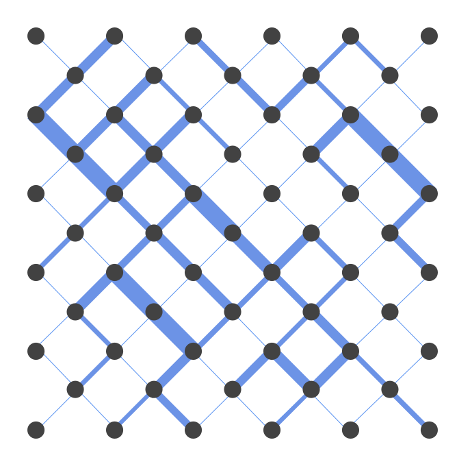
The considered network has $500\times 500$ nodes and the link length, $l$, is equal for all links. All links are oriented at $\pm\pi/4$ radians with respect to the horizontal direction. In each realization of this structured network $1000$ tracer particles are injected in the center of the left boundary and tracked in the domain and $1000$ such realization are considered. No-flow boundary conditions are set on the top and bottom of the domain, and a mean pressure gradient is imposed by setting the pressure at the left and right boundaries. Each realization of the medium is obtained by drawing the transmissibility of each link independently from a log-normal distribution with variance $\sigma^{2}=5$. The flow problem is first solved for each realization and the velocity field is obtained. We then simulate the transport of a passive tracer using particle tracking. Here, diffusion inside the links is neglected and perfect mixing is assumed inside the nodes. At each node, the particle randomly chooses a link carrying flux out of that node with a probability proportional to the flux in that link.

The outputs of this particle tracking procedure are $x_{n}^{(i)}$ and $y_{n}^{(i)}$ and $t_{n}^{(i)}$, where $x_{n}^{(i)}$ and $y_{n}^{(i)}$ are the position coordinates of particle $i$ after $n$ transitions and $t_{n}^{(i)}$ is the elapsed time to get to that position. Given these trajectories for all particles, we can obtain the ensemble concentration of the contaminant at a given time less than $\min_{i}\max_{n}t_{n}^{(i)}$, which is the largest time where none of the particles has left the domain. Alternatively, one can obtain the distribution of the first passage time (FPT) for a certain $x_{t}$ plane.

To describe the average movement of the particle plume we analyze the Lagrangian statistics of the particles along each trajectory. As described in the previous section, we assume the velocity process is stationary and model the velocity of the particles, $\mathbf{v}_{n}^{(i)}$, by a Markov process. One can use the velocities obtained directly from the MC transport simulations $(x_{n}^{(i)},y_{n}^{(i)},t_{n}^{(i)})$. That is,

$$\begin{gathered}\mathbf{v}_{n}^{(i)}=[v_{x}^{(i)},v_{y}^{(i)}]_{n}^{T},\\ v_{x}^{(i)}=\frac{x_{n+1}^{(i)}-x_{n}^{(i)}}{t_{n+1}^{(i)}-t_{n}^{(i)}}\text{ and }v_{y}^{(i)}=\frac{y_{n+1}^{(i)}-y_{n}^{(i)}}{t_{n+1}^{(i)}-t_{n}^{(i)}}.\end{gathered}$$ (4)

A Markov model based on these velocities would allow us to efficiently march particles with length steps equal to $l$. This would correspond to a spatial Markov model. One can imagine that $l$ is typically much smaller than the length scales of practical interest, and we might not be interested in the details of the particle path after each transition to a new node in the network. In the next section the proposed temporal Markov model is discussed.

5 Stencil method: the temporal Markov model

A temporal Markov model for the velocity process described in the previous section would require computing the average particle velocity in a sequence of given time intervals. If the averaging time step is larger than the mean time required for one transition, by combining multiple transitions together, averaging will increase the numerical efficiency of the temporal Markov model. Moreover, there is no distinction between structured and unstructured networks when obtaining the average velocity process; therefore, averaging would also generalize the model to unstructured networks. We refer to the averaging time step, $\Delta t_{s}$, as the stencil time.

We represent the average velocity $\overline{\mathbf{v}}_{n}^{(i)}$ over a time period of $\Delta t_{s}$ in polar coordinates by its magnitude and the angle $\overline{\theta}_{n}^{(i)}$ between its direction and the unit vector in the $x$ direction. Here the subscript $n$ refers to the $n$’th time step. The average velocity and average angle are divided into discrete classes as follows:

$$\begin{gathered}v\in\cup_{j=1}^{n_{v}}(log(\overline{v})_{j},log(\overline{v})_{j+1})\\ \text{and }\theta\in\cup_{j=1}^{n_{\theta}}(\overline{\theta}_{j},\overline{\theta}_{j+1}),\end{gathered}$$ (5)

where $n_{v}$ and $n_{\theta}$ are the number of velocity magnitude and angle classes. As previously suggested in [21, 16], in order to better represent slow transitions we use the logarithm of velocity magnitude for the definition of classes. The state of a particle velocity is defined by a $({v},{\theta})$-pair. We refer to this temporal model as the velocity-angle stencil method, or the stencil method.

Similar to the polar Markovian velocity process (PMVP)  [24, 35], the velocity-angle stencil is based on polar coordinates. Unlike the PMVP, the velocity and angle processes are not considered separately, i.e., they are jointly modeled by one stochastic process in time. Moreover, the PMVP is a combination of a spatial and a temporal SDE. The stencil method is a discrete temporal Markov chain. The advantage of using a discrete Markov chains is that no assumptions are needed for the functional form of the transition probabilities.

Compared to the correlated spatial models that follow every particle transition on the network (e.g., the one by Kang et al. [16]), the velocity-angle stencil method has two limitations. First, since we are using average trajectories, collisions (velocity transitions) do not coincide with the nodes of the underlying physical network. In order to inform the model about the exact location of the collision, a new variable, $\tau$, can be added to track the time between the end of every averaging instant and the next collision event. This idea has been discussed in Jenny and Meyer [32] and it is not discussed further here. Another limitation of the velocity-angle stencil is its inaccuracy in case of very slow transitions, i.e., if $\Delta t_{n}^{(i)}=t_{n+1}^{(i)}-t_{n}^{(i)}\gg\Delta t_{s}$. This has been noted previously in [14, 23]. Averaging such time steps would result in many consecutive steps where the velocity state would remain unchanged. 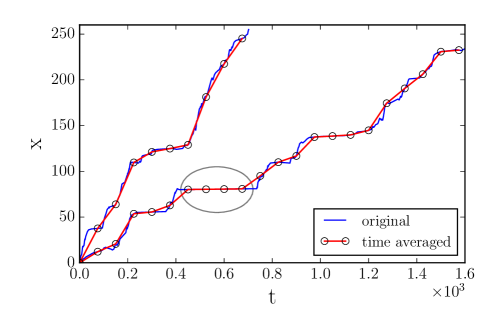However, using the velocity-angle stencil, the particle is allowed to change its velocity after every $\Delta t_{s}$, and this could limit the persistence of the low velocities and make the model less accurate. Figure 2 shows the trajectory of two sample particles and the averaged trajectories for the same particles for the same number of jumps. The circled section illustrates an example of a particle experiencing a relatively low velocity.

Figure 2: Sample trajectory of two particles. Solid blue: original particle path, markers: trajectory resulting from average velocities. The circled area illustrates an example of a particle experiencing a relatively low velocity.

Next, we discuss a method for overcoming the limitation due to very slow transition by enriching the state space of the stencil model. When averaging the particle trajectories with a stencil time step $\Delta t_{s}$, the number of repetitions, denoted by $f$, during a time step is known. This information can be added to the definition of the particle state. By having the collision frequency in the state definition, it becomes possible to accurately model particles that stay in a low-velocity state for long time intervals. With this new state definition, the attributes of the particle state are $({v},{\theta},f)$. We refer to this model as the extended velocity-angle stencil method or the extended stencil method.

6 Model calibration and validation of the Markov property

Similar to Kang et al. [16], we use equal probability bins for the log-velocity classes. Due to averaging, the angle process takes continuous values in $[-\pi,\pi]$ and will include values that do not coincide with the initial network link directions. We use equal-width bins for the velocity angle classes. In the extended stencil method, for each observed frequency in the input data, a separate class was allocated for the corresponding $(v,{\theta})$ pair. We refer to the discrete transition matrix for the stencil method as $p_{m}(v,{\theta}|v^{\prime},{\theta}^{\prime})$. This is the probability of encountering the state $(v,{\theta})$ after $m$ transitions, assuming that we started from the state $(v^{\prime},{\theta}^{\prime})$. Similarly $p_{m}(v,{\theta},f|v^{\prime},{\theta}^{\prime},f^{\prime})$ is the discrete transition matrix for the extended stencil method. Both transition matrices were obtained by counting the observed transitions in the particle tracking simulation results, which corresponds to the maximum likelihood estimation of the transition probabilities. We also define the aggregate velocity transition matrix $T_{m}^{v}(i,j)$, which defines the probability of encountering velocity class $i$ after $m$ transitions starting from velocity class $j$, and the aggregate angle transition matrix $T_{m}^{\theta}(i,j)$, which is defined in a similar way. The mean transition time observed in the particle tracking data, $\overline{\delta t}$, is considered as a time scale.

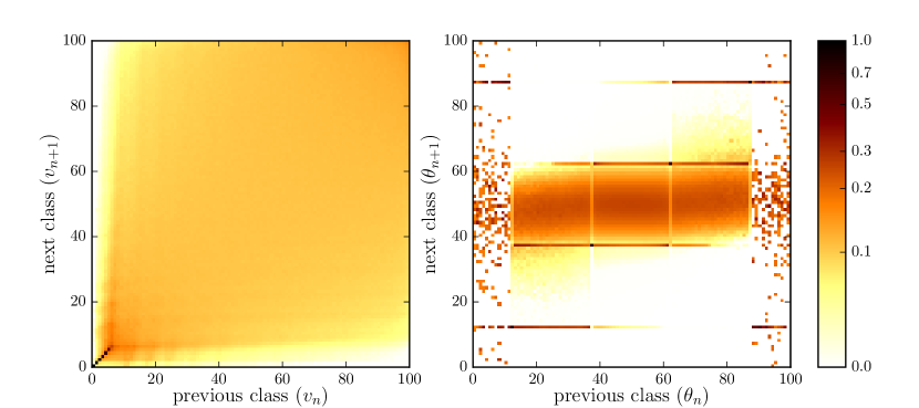
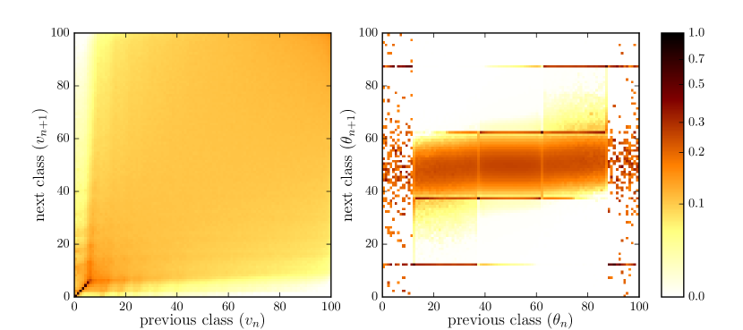
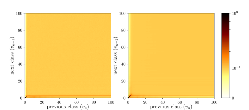
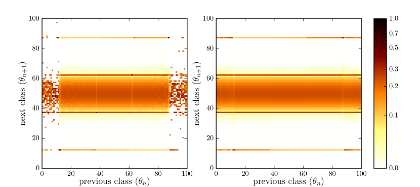
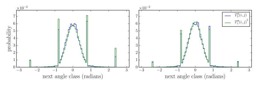
The aggregate velocity and angle transition matrices for one transition with $\Delta t_{s}=10\overline{\delta t}$ for the stencil method and the extended stencil method are shown in Figs. 3 and 4. The transition matrices for these two models will be different, since repeating $(v,\theta)$ pairs are counted as a transition to the same state in the stencil method, which is not the case for the extended velocity-angle stencil. The resulting aggregate transition matrices are almost identical except for the lower left corner of the velocity transition matrices. Provided that a Markov process can closely model transitions between different states, we expect that the Chapman-Kolmogorov relation [36] holds for these transitions. We perform a test to compare the m-step aggregate transition matrices for $v$ and $\theta$ with the m-fold product of the corresponding one-step transition matrices. 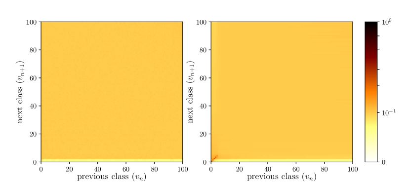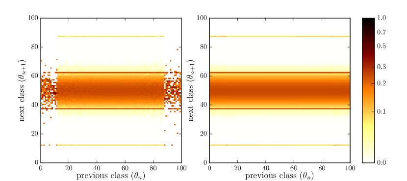The aggregate five-step velocity transition matrix $T_{5}^{v}(i,j)$ and the aggregate five-step angle transition matrix $T_{5}^{\theta}(i,j)$ are compared to ${T_{1}^{v}(i,j)}^{5}$ and ${T_{1}^{\theta}(i,j)}^{5}$ from the stencil method in Figs. 5 and 6 for $\Delta t_{s}=10\overline{\delta t}$. The same comparison is performed for the extended-stencil method and presented in Figs. 7 and 8. As can be seen from these four figures, the Chapman-Kolmogorov relation approximately holds for all angles and for velocity classes with $j>5$.

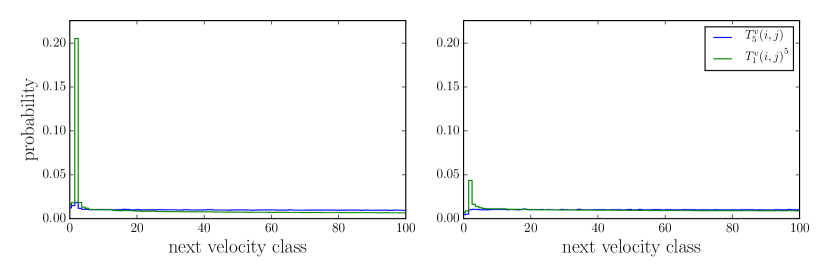
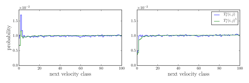
A column-wise comparison of the aggregate angle transition matrices for an angle in the second quarter ($j=78$) is shown in Fig. 9. Since the mean-flow directions is from left to right ($\theta=0$), there are not that many sample paths with velocity angles close to $\pi$ or $-\pi$. This explains the noise observed in the aggregate angle transition matrices of Figs. 3 and 4. The column-wise comparison of the aggregate velocity transition matrices for a low velocity class ($j=2$) and a high velocity class ($j=98$) are shown in Figs. 10 and 11. Although there is a clear deviation from Markovianity for both the stencil method and the extended stencil method, these results suggest that enriching the state space of the Markov model would result in significantly better predictions of transitions from extremely low velocity values. This is best illustrated in Fig. 10. The extended velocity-angle stencil also improves the predicted lag five transitions from a fast velocity class to slow velocity classes as seen in Fig. 11.

Similar comparisons were performed for larger stencil times, $\Delta t_{s}>10\overline{\delta t}$, for both the stencil method and the extended stencil method. For these larger stencil times both models lead to smaller errors in predicting the five-step transition probabilities. This is expected, since with larger stencil times we are combining more transitions and consecutive transitions become less correlated and hence less challenging to predict for the Markov models. In the limit of $\Delta t_{s}\rightarrow\infty$ we expect the average velocity distribution to converge to an equilibrium distribution and every column of the transition matrices would be equal to the corresponding equilibrium distribution. Hence, for very large $\Delta t_{s}$ the one-point distribution of $\overline{v}$ would be sufficient for modeling dispersion. The choice of $\Delta t_{s}$ would also depend on the temporal resolution of interest. The range of stencil times where a correlated stencil is required for accurate predictions of contaminant transport is further discussed in section 7.

For $\Delta t_{s}<10\overline{\delta t}$, both the velocity-angle stencil and the extended velocity-angle stencil lead to errors in predicting the transition probabilities for a larger set of velocity classes. However, from a computational point of view we are not interested in these stencil times, since by combining very few transitions, only small speed-ups can be expected compared to correlated spatial models. In case we are interested in these smaller time steps, the right tool has already been developed (correlated CTRW). The resulting plumes and first passage time curves predicted by these smaller stencil times are included in section 7.

Figure 3: Left: aggregate velocity transition matrix for $m=1$, $T_{1}^{v}(i,j)$; right: aggregate angle transition matrix for $m=1$, $T_{1}^{\theta}(i,j)$ for the velocity-angle stencil for $\Delta t_{s}=10\overline{\delta t}$. The square root of the values are plotted in logarithmic scale.

Figure 4: Left: aggregate velocity transition matrix for $m=1$, $T_{1}^{v}(i,j)$; right: aggregate angle transition matrix for $m=1$, $T_{1}^{\theta}(i,j)$ for the extended velocity-angle stencil for $\Delta t_{s}=10\overline{\delta t}$. The square root of the values are plotted in logarithmic scale.

Figure 5: Verification of the Chapman-Kolmogorov relation for velocity-magnitude classes for the stencil method for $\Delta t_{s}=10\overline{\delta t}$; left: $T_{5}^{v}(i,j)$; right: ${T_{1}^{v}(i,j)}^{5}$. The square root of the values are plotted in logarithmic scale.

Figure 6: Verification of the Chapman-Kolmogorov relation for the velocity-angle classes for the stencil method for $\Delta t_{s}=10\overline{\delta t}$; left: $T_{5}^{\theta}(i,j)$; right: ${T_{1}^{\theta}(i,j)}^{5}$. The square root of the values are plotted in logarithmic scale.

Figure 7: Verification of the Chapman-Kolmogorov relation for velocity-magnitude classes for the extended stencil method for $\Delta t_{s}=10\overline{\delta t}$; left: $T_{5}^{v}(i,j)$; right: ${T_{1}^{v}(i,j)}^{5}$. The square root of the values are plotted in logarithmic scale.

Figure 8: Verification of the Chapman-Kolmogorov relation for the velocity-angle classes for the extended stencil method for $\Delta t_{s}=10\overline{\delta t}$; left: $T_{5}^{\theta}(i,j)$; right: ${T_{1}^{\theta}(i,j)}^{5}$. The square root of the values are plotted in logarithmic scale.

Figure 9: Column-wise comparison of $T_{5}^{\theta}(i,j)$ and ${T_{1}^{\theta}(i,j)}^{5}$ for an initial angle in the second quarter with $j=78$ for $\Delta t_{s}=10\overline{\delta t}$; left: stencil method; right: extended stencil method.

Figure 10: Column-wise comparison of $T_{5}^{v}(i,j)$ and ${T_{1}^{v}(i,j)}^{5}$ for a slow initial velocity class with $j=2$ for $\Delta t_{s}=10\overline{\delta t}$; left: stencil method; right: extended stencil method.

Figure 11: Column-wise comparison of $T_{5}^{v}(i,j)$ and ${T_{1}^{v}(i,j)}^{5}$ for a fast initial velocity class with $j=98$ for $\Delta t_{s}=10\overline{\delta t}$; left: stencil method; right: extended stencil method.

The results presented in this section indicate that the transition probabilities of the MC data are not strictly Markovian for any $\Delta t_{s}$, which is consistent with the findings of Le Borgne et al. [14]. However, we do not expect an exact Markovian structure in the MC results to begin with. For example, the MC results indicate that in every realization there are fast paths between the two ends of the domain, and knowing the full history of the velocity of a particle would improve our prediction of whether that particle is in a preferential path or not. This clearly indicates that the velocity process is not strictly Markovian. Therefore, although verifying the Chapman-Kolmogorov relation gives us useful intuition about the value of a Markov assumption for this problem, the usefulness of this assumption needs to be judged by the predictive power of the model and the error induced due to this assumption. In the next section, numerical results from both stencil models are presented and compared to the particle ensemble from the particle tracking simulations.

7 Numerical results

Different velocity-angle stencils and extended velocity-angle stencils were obtained for different averaging times and the average transport in the network was compared with the predictions of the stencil methods. The performance of the stencil models were compared to an implementation of the correlated CTRW method. The code for generating the MC data and performing these comparisons is available at https://github.com/amirdel/dispersion-random-network [37]. First, we present results for $\Delta t_{s}=20\overline{\delta t}$. The results for smaller and larger time steps are discussed afterwards.

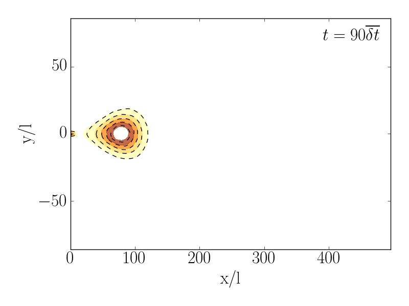
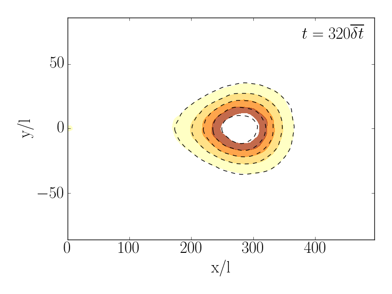
First, we consider the velocity-angle stencil. Figs. 12 and 13 show the particle plume and the predicted plume by the velocity-angle stencil at dimensionless times $t/\overline{\delta t}=90$ and $320$, respectively. As these figures suggest, the stencil model captures the distribution of the tracer with great accuracy and the non-Gaussian characteristics of the plume are well captured using this simpler model. 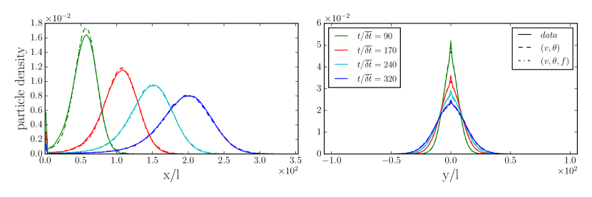The same contaminant plume was also simulated with the extended stencil model. In Fig. 14 the results from both models are compared to the reference concentration distributions from the particle tracking simulations. 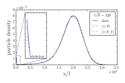Both models capture the spreading of the plume accurately for different times in both longitudinal and transverse directions. When magnifying the slow tail of the plume in Fig. 15, it is observed that the extended stencil captures this slow tail better than the velocity-angle stencil.

Figure 12: Contaminant concentration at non-dimensional time $t/\overline{\delta t}=90$. Comparison of the velocity-angle stencil (dashed lines) with the reference particle tracking data (filled contour map) for the same contour levels.

Figure 13: Contaminant concentration at non-dimensional time $t/\overline{\delta t}=320$. Comparison of the velocity-angle stencil (dashed lines) with the reference particle tracking data (filled contour map) for the same contour levels.

Figure 14: Comparison of plume concentration at different times: particle tracking data (solid lines), velocity-angle stencil (dashed lines), extended velocity-angle stencil (dash dots). Stencil time is $20\overline{\delta t}$ for both models.

Figure 15: Comparison of plume concentration at $t/\overline{\delta t}=320$: particle tracking data (solid lines), velocity-angle stencil (dashed lines), extended velocity-angle stencil (dash dots). Inset: zooming on the slow tail of the plume.

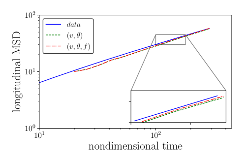
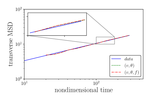
The second central moment of the particle plume or the mean square displacement (MSD), with respect to the plume center of mass in the longitudinal directions obtained from the temporal Markovian models is compared to the MSD obtained from the ensemble plume in Fig. 16. It can be observed that the predictions from both models are very similar. A closer inspection (inset of Fig. 16) illustrates that the extended stencil method improves the predictions of the longitudinal MSD. A similar comparison is shown for the transverse direction in Fig. 17. The results show that using the extended class definition does not improve the predictions of the second moment in the transverse direction.

Figure 16: Comparison of longitudinal mean square difference of the plume at different times: particle tracking data (solid lines), velocity-angle stencil (dashed lines), extended velocity-angle stencil (dash dots). Stencil time is $20\overline{\delta t}$ for both models.

Figure 17: Comparison of traverse mean square difference of the plume for different times: particle tracking data (solid lines), velocity-angle stencil (dashed lines), extended velocity-angle stencil (dash dots). Stencil time is $20\overline{\delta t}$ for both models.

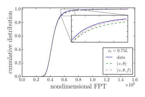
Another important feature of anomalous transport is the long tail in first passage time (FPT) distributions. Figure 18 shows the comparison of the FPT for non-dimensional length $x_{t}/L=0.75$, where $x_{t}$ is the target $x$ plane and $L$ is the domain length. The long tail of the first passage time CDF is well captured by both stencil models. This comparison was performed for $x_{t}/L=0.25$, $0.5$ and $0.75$, and the predictions from both models are accurate for all three planes. A closer inspection of the FPT curve (Fig. 18) illustrates that the extended class definition improves the prediction of the FPT distribution.

Figure 18: First passage time CDF for $x/L=0.75$: particle tracking data (solid lines), velocity-angle stencil (dashed lines), extended velocity-angle stencil (dash dots) for $\Delta t_{s}=20\overline{\delta t}$.

Although the extended stencil results in more accurate predictions for $\Delta t_{s}=20\overline{\delta t}$, the improvements can be better observed for smaller stencil times. Figure 19 indicates that there is a significant difference between the predictions of the stencil model and the extended stencil model for a wide range of first passages times. Most notably, the slow tail of the FPT curve is captured well with the extended stencil method even for very small stencil times. 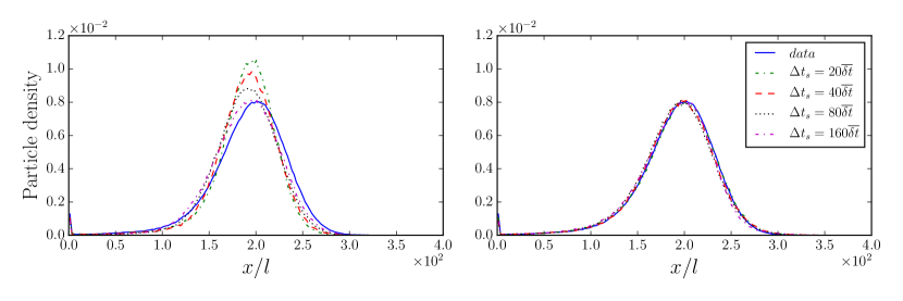Hence, by using the extended stencil we were able to expand the range of accuracy of temporal Markov models to smaller time steps. In Fig. 20 the plumes predicted by the two stencil models are compared for small stencil times. Although the predictions are not as accurate as in the case with $\Delta t_{s}=20\overline{\delta t}$, for $\Delta t_{s}=10\overline{\delta t}$ there still is a good agreement between the model predictions and the MC simulation results. For smaller stencil times, the extended velocity-angle stencil leads to smaller errors, especially for the slow tail of the plume.

Figure 19: First passage time CDF for $x/L=0.75$ for different stencil times; left: stencil method; right: extended stencil method.

Figure 20: Particle density at $t/\overline{\delta t}=320$ for different stencil times; left: stencil method; right: extended stencil method.

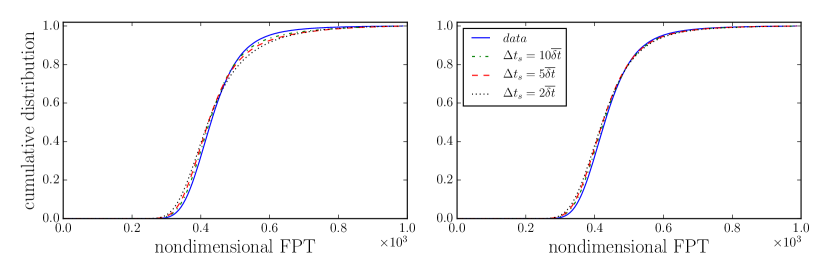
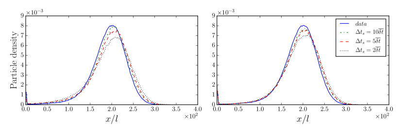
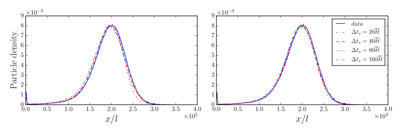
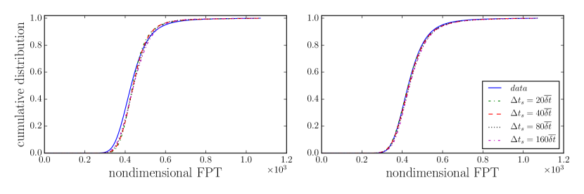
Given the same MC simulation data, with larger averaging windows there would be fewer velocity transitions along every streamline and converging to the correct discrete transition matrix would become harder. Figures 21 and 22 show the predicted plume and the FPT curve for $\Delta t_{s}$ equal to $20$, $40$, $80$, $160$ times $\overline{\delta t}$ for both stencil methods. As can be seen in these figures, both models make similar predictions and capture the dispersion process well for stencil times up to $\Delta t_{s}=80\overline{\delta t}$. For the largest stencil time ($\Delta t_{s}=160\overline{\delta t}$) the extended stencil clearly leads to more accurate predictions. One should note that for very large stencil times, the MC data is not sufficient to obtain statistical convergence of the transition matrices. This is due to having only a few velocity transitions per particle trajectory. However, the extended stencil by construction can capture the extremely slow tail of the plume more accurately; this advantage is reflected in the predicted probability densities and FPT curves.

On the other hand, with larger stencil times the average velocities would become less correlated. One can argue that with very large stencil times, using a correlated random walk model would no longer be necessary and independent spatial increments would be sufficient for modeling the dispersion process at very low temporal resolutions. Figures 23 and 24 compare the results of using an uncorrelated temporal random walk for predicting the FPT and the particle concentration PDF with the results of the extended stencil model. These results suggest that for a wide range of stencil times ($20<\Delta t_{s}/\overline{\delta t}<160$) considering the velocity correlation is indeed necessary for making accurate predictions.

Figure 21: Predicted plume concentration for different values of $\Delta t_{s}/\overline{\delta t}$; left: stencil method; right: extended stencil method.

Figure 22: FPT curve for different values of $\Delta t_{s}/\overline{\delta t}$; left: stencil method; right: extended stencil method.

Figure 23: Predicted plume concentration for different values of $\Delta t_{s}/\overline{\delta t}$, left: using uncorrelated average velocities; right: extended stencil method.

Figure 24: FPT curve for different values of $\Delta t_{s}/\overline{\delta t}$, left: using uncorrelated average velocities; right: extended stencil method.

The computational cost of the stencil method was compared to correlated CTRW with spatial transitions that are equal to the link lengths in the network [16]. The cost is computed by counting the average number of velocity transitions along a particle trajectory before exiting the domain. A stencil model with $\Delta t_{s}=\alpha\overline{\delta t}$, with $\alpha>10$, leads to $\alpha$ times less collisions compared with following every transition to a new node; therefore, it is $\alpha$ times computationally more efficient. For temporal models with $\Delta t_{s}<10\overline{\delta t}$, the stencil method is less accurate than correlated CTRW and does not offer significant computational gains.
The transition matrices for both the stencil method and the extended stencil method are stored in sparse format which results in efficient use of memory. For more details regarding the model implementation please refer to the provided repository.

8 Application to unstructured networks

The proposed stencil methods require no further generalizations to model transport in unstructured networks. In contrast, published correlated spatial models used for simulating transport in structured networks are different from the models applied to unstructured networks. In [19], independent spatial Markov processes are used for each spatial dimension, and in [20] the analysis of unstructured fracture networks is limited to the projection of the particle velocities on the longitudinal direction. 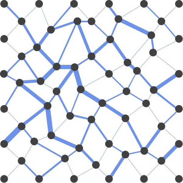Here we illustrate that the proposed temporal models are readily applicable to unstructured cases. To this end, unstructured networks were generated by randomly perturbing the nodes in the structured network used in the previous section. Normal random perturbations were added independently in the horizontal and vertical directions. A schematic of such a resulting unstructured network is shown in Fig. 25. This procedure would result in unstructured networks with a truncated Gaussian link length distribution. The link length distribution for four such networks are depicted in Fig. 26.

Figure 25: Schematic of an unstructured network generated by adding normal random perturbations to a zig zag structured network.

Figure 26: Link length distribution from four realizations of the studied random unstructured network.

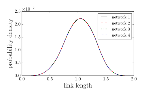
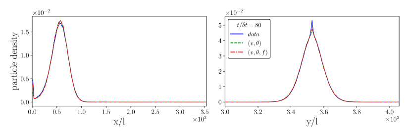
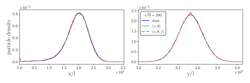
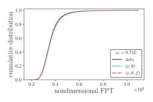
The same particle tracking problem described in section 4 was performed on $1000$ realizations of these unstructured networks and the problem was also modeled using both the velocity-angle and the extended velocity-angle stencils. Figures 27 and 28 show the plume spreading for two different times. These results show that the stencil model can also be used to accurately predict contaminant plume spreading in unstructured networks. Figure 29 shows that the early and late particle arrival times are also captured accurately for this test case.

Figure 27: Longitudinal (left) and transverse (right) distributions of the plume at $t/\overline{\delta t}=80$ for the unstructured random network test case with $\Delta t_{s}=20\overline{\delta t}$.

Figure 28: Same as Fig. 27, at a later time.

Figure 29: First passage time CDF for $x_{t}=0.75L$ for the unstructured random network example.

9 Conclusions

In this work, we showed that temporal Markov models can be used to model transport in random networks with good accuracy for a wide range of stencil times. Although it is known that using temporal Markov models can lead to wrong transition rates both from and to low-velocity states, it was shown that the error induced due to this fact is in many cases small, and can be further reduced by using the extended velocity-angle stencil. We were able to improve the results obtained by temporal Markov models by enriching the state space of the model to include information on the number of repetitions of a given velocity class and extend the range of applicability of these models to smaller time steps. The extended stencil enhanced the accuracy of predicting the slow tail of the contaminant plume, the CDF of first passage time, and the evolution of the second central moment of the plume in the longitudinal direction. We also showed that discrete temporal Markov models can be used to model transport in unstructured networks without any further modification. Moreover, since many node transitions can be treated collectively in one stencil step, the proposed stencil method is more efficient than simulating particle evolution based on following every transition to a new node. Compared to previously proposed temporal Markov models based on SDEs, the models proposed here make significantly fewer modeling assumptions. Applying the stencil method to correlated heterogeneous fields will be the subject of further studies.

References

- Berkowitz et al. [2006] Berkowitz B, Cortis A, Dentz M, Scher H. Modeling non-fickian transport in geological formations as a continuous time random walk. Reviews of Geophysics 2006;44(2).
- Bouchaud and Georges [1990] Bouchaud JP, Georges A. Anomalous diffusion in disordered media: statistical mechanisms, models and physical applications. Physics reports 1990;195(4-5):127–293.
- Edery et al. [2014] Edery Y, Guadagnini A, Scher H, Berkowitz B. Origins of anomalous transport in heterogeneous media: Structural and dynamic controls. Water Resources Research 2014;50(2):1490–505.
- Nowak et al. [2012] Nowak W, Rubin Y, Barros FP. A hypothesis-driven approach to optimize field campaigns. Water Resources Research 2012;48(6).
- Moslehi and de Barros [2017] Moslehi M, de Barros FP. Uncertainty quantification of environmental performance metrics in heterogeneous aquifers with long-range correlations. Journal of Contaminant Hydrology 2017;196:21–9.
- Ghorbanidehno et al. [2015] Ghorbanidehno H, Kokkinaki A, Li JY, Darve E, Kitanidis PK. Real-time data assimilation for large-scale systems: The spectral kalman filter. Advances in Water Resources 2015;86:260–72.
- Li et al. [2015] Li JY, Kokkinaki A, Ghorbanidehno H, Darve EF, Kitanidis PK. The compressed state kalman filter for nonlinear state estimation: Application to large-scale reservoir monitoring. Water Resources Research 2015;.
- Ghorbanidehno et al. [2017] Ghorbanidehno H, Kokkinaki A, Kitanidis PK, Darve E. Optimal estimation and scheduling in aquifer management using the rapid feedback control method. Advances in Water Resources 2017;110:310–8.
- Fiori et al. [2015] Fiori A, Zarlenga A, Gotovac H, Jankovic I, Volpi E, Cvetkovic V, Dagan G. Advective transport in heterogeneous aquifers: Are proxy models predictive? Water resources research 2015;51(12):9577–94.
- Banton et al. [1997] Banton O, Delay F, Porel G. A new time domain random walk method for solute transport in 1–d heterogeneous media. Ground Water 1997;35(6):1008–13.
- Bodin et al. [2003] Bodin J, Porel G, Delay F. Simulation of solute transport in discrete fracture networks using the time domain random walk method. Earth and Planetary Science Letters 2003;208(3):297–304.
- Graham and McLaughlin [1989] Graham W, McLaughlin D. Stochastic analysis of nonstationary subsurface solute transport: 1. unconditional moments. Water Resources Research 1989;25(2):215–32. URL: http://dx.doi.org/10.1029/WR025i002p00215. doi:10.1029/WR025i002p00215.
- Le Borgne et al. [2007] Le Borgne T, de Dreuzy JR, Davy P, Bour O. Characterization of the velocity field organization in heterogeneous media by conditional correlation. Water resources research 2007;43(2).
- Le Borgne et al. [2008a] Le Borgne T, Dentz M, Carrera J. Lagrangian statistical model for transport in highly heterogeneous velocity fields. Physical review letters 2008a;101(9):090601.
- Le Borgne et al. [2008b] Le Borgne T, Dentz M, Carrera J. Spatial markov processes for modeling lagrangian particle dynamics in heterogeneous porous media. Physical Review E 2008b;78(2):026308.
- Kang et al. [2011] Kang PK, Dentz M, Le Borgne T, Juanes R. Spatial markov model of anomalous transport through random lattice networks. Physical review letters 2011;107(18):180602.
- Kang et al. [2015a] Kang PK, Dentz M, Le Borgne T, Juanes R. Anomalous transport on regular fracture networks: Impact of conductivity heterogeneity and mixing at fracture intersections. Physical Review E 2015a;92(2):022148.
- Kang et al. [2015b] Kang PK, Le Borgne T, Dentz M, Bour O, Juanes R. Impact of velocity correlation and distribution on transport in fractured media: Field evidence and theoretical model. Water Resources Research 2015b;51(2):940–59.
- Kang et al. [2014] Kang PK, De Anna P, Nunes JP, Bijeljic B, Blunt MJ, Juanes R. Pore-Scale intermittent velocity structure underpinning anomalous transport through 3-D porousmedia. Geophysical Research Letters 2014;41(17):6184–90. doi:10.1002/2014GL061475.
- Kang et al. [2017] Kang PK, Dentz M, Le Borgne T, Lee S, Juanes R. Anomalous transport in disordered fracture networks: spatial markov model for dispersion with variable injection modes. Advances in Water Resources 2017;.
- Meyer and Tchelepi [2010] Meyer DW, Tchelepi HA. Particle-based transport model with markovian velocity processes for tracer dispersion in highly heterogeneous porous media. Water Resources Research 2010;46(11).
- Meyer et al. [2010] Meyer DW, Jenny P, Tchelepi HA. A joint velocity-concentration pdf method for tracer flow in heterogeneous porous media. Water Resources Research 2010;46(12).
- Meyer and Saggini [2016] Meyer DW, Saggini F. Testing the markov hypothesis in fluid flows. Physical Review E 2016;93(5):053103.
- Meyer et al. [2013] Meyer DW, Tchelepi HA, Jenny P. A fast simulation method for uncertainty quantification of subsurface flow and transport. Water Resources Research 2013;49(5):2359–79.
- Meyer and Bijeljic [2016] Meyer DW, Bijeljic B. Pore-scale dispersion: Bridging the gap between microscopic pore structure and the emerging macroscopic transport behavior. Physical Review E 2016;94(1):013107.
- Attinger et al. [2004] Attinger S, Dentz M, Kinzelbach W. Exact transverse macro dispersion coefficients for transport in heterogeneous porous media. Stochastic Environmental Research and Risk Assessment 2004;18(1):9–15.
- Blunt et al. [2002] Blunt MJ, Jackson MD, Piri M, Valvatne PH. Detailed physics, predictive capabilities and macroscopic consequences for pore-network models of multiphase flow. Advances in Water Resources 2002;25(8):1069–89.
- Dong and Blunt [2009] Dong H, Blunt MJ. Pore-network extraction from micro-computerized-tomography images. Physical review E 2009;80(3):036307.
- Khayrat and Jenny [2016] Khayrat K, Jenny P. Subphase approach to model hysteretic two-phase flow in porous media. Transport in Porous Media 2016;111(1):1–25.
- Mehmani and Tchelepi [2017] Mehmani Y, Tchelepi HA. Minimum requirements for predictive pore-network modeling of solute transport in micromodels. Advances in Water Resources 2017;.
- Delgoshaie et al. [2015] Delgoshaie AH, Meyer DW, Jenny P, Tchelepi HA. Non-local formulation for multiscale flow in porous media. Journal of Hydrology 2015;531:649–54.
- Jenny and Meyer [2016] Jenny P, Meyer D. Non-local generalization of darcy’s law based on empirically extracted conductivity kernels. In: ECMOR XV-15th European Conference on the Mathematics of Oil Recovery. 2016:.
- Kang et al. [2016] Kang PK, Brown S, Juanes R. Emergence of anomalous transport in stressed rough fractures. Earth and Planetary Science Letters 2016;454:46–54.
- Painter and Cvetkovic [2005] Painter S, Cvetkovic V. Upscaling discrete fracture network simulations: An alternative to continuum transport models. Water Resources Research 2005;41(2).
- Dünser and Meyer [2016] Dünser S, Meyer DW. Predicting field-scale dispersion under realistic conditions with the polar markovian velocity process model. Advances in Water Resources 2016;92:271–83.
- Resnick [2013] Resnick SI. Adventures in stochastic processes. Springer Science & Business Media; 2013.
- Delgoshaie [2018] Delgoshaie AH. amirdel/dispersion-random-network: random network. 2018. URL: https://doi.org/10.5281/zenodo.1213380. doi:10.5281/zenodo.1213380.