Probing BAO studies with flat $\Lambda$CDM constraints

Abstract

One of the algorithms typically used for fitting anisotropic Baryon Acoustic Oscillations (BAO), $\alpha_{\perp}D_{M,\text{fid}}(z)/r_{d,\text{fid}}=D_{M}(z)/r_{d}$, provides an excellent fit as $z\Rightarrow 0$. Yet, at $z_{\text{drag}}\simeq 1060$, $D_{M,\text{fid}}(1060)/r_{d,\text{fid}}\simeq D_{M}(1060)/r_{d}$. Since $\alpha_{\perp}$ does not change with increasing redshift, we conclude that the algorithms deviate from true solutions with increasing $z$. We investigate that departure through an assumption of a flat $\Lambda$CDM cosmology. At the relatively low redshifts at which isotropic BAO studies were performed, the divergence is smaller than study uncertainties. However, while the transverse measure, $\alpha_{\perp}$ provides a reliable value in real space, not corrupted by redshift distortion, the isotropic measure, $\alpha$, has a radial component, and is influenced by redshift distortion. That distortion recommends against the inclusion of isotropic studies in cosmological parameter evaluations. At the high redshifts of Ly$\alpha$ forest BAO studies, $z\sim$ 2.35, the deviations of the anisotropic BAO algorithms from the flat $\Lambda$CDM solutions give rise to markedly deceptive results. We replicate an example, in which those algorithms lead to a value of $\Omega_{m}$ which is more than 15 per cent lower than that of the flat $\Lambda$CDM cosmology computation. The BAO algorithms are inappropriate for the next generation of BAO studies. A flat $\Lambda$CDM analysis offers an alternative means of assessment.

1 Introduction

Baryon Acoustic Oscillation (BAO) findings taken together with cosmic microwave background (CMB) results significantly restrict the $\Omega_{m}$, $H_{0}$, confidence interval. CMB satellite missions have applied that joint characteristic (Spergel et al., 2007; Komatsu et al., 2011; Hinshaw et al., 2013; Planck 2013 results XVI, 2014; Planck 2015 results XIII, 2016; Planck 2018 results VI, 2018) since the first successful statistical recoveries (Eisenstein et al., 2005; Cole et al., 2005) of the BAO acoustic scale. Addison et al. (2013, 2018) performed analyses of ensembles of several BAO studies, constraining cosmological parameters, and probing the CMB versus low redshift measurement discrepancy of the Hubble constant, and Aubourg et al. (2015) have employed a set of BAO studies to survey variations from a flat, $w$=-1, $\Lambda$CDM universe.

Evaluations of the BAO feature from the two point correlation function (2PCF) have attained a precision of $\sim$1 percent, (see, e.g, Cuesta et al. (2016)). Projects recently initiated, Dark Energy Spectroscopic Instrument (DESI) (Vargas-Magaña, et al., 2019), and further in the future, Euclid, (Euclid Collaboration, 2019), and the Wide Field Infra Red Space Telescope (WFIRST) (Doré, et al., 2019) will attain sub-percent precision levels. With that improved precision in mind, we explore BAO methodology with the intent of identifying uncertainties that might limit attainable precision.

At this juncture, precise CMB measurements, together with gravitational lensing, have restricted variation from flatness to $\Omega_{K}=-0.012^{+0.021}_{-0.023}$, (Simard et al., 2018), and combined CMB and SNe Ia measurements constrain $w$ to $-1.02\pm{0.06}$ (Betoule et al., 2014). We rely on these restrictions to justify an analysis of BAO results, in which we set $\Omega_{K}=0$ and $w=-1$. That flat $\Lambda$CDM model scaffolding facilitates the derivation of cosmological parameter values from the BAO studies. Percival et al. (2002) derived an expression, $\Omega_{m}h^{3}$=constant, which describes the $\Omega_{m}$, $H_{0}$ near-degeneracy within the flat cosmology, where the dimensionless parameter, h, is used to define the Hubble constant, $H_{0}=100h$ km $\text{s}^{-1}$ $\text{Mpc}^{-1}$. The Planck mission provides a premium data set, from which we extract their value of the constant (Planck 2018 results VI, 2018),

$$\Omega_{m}h^{3}=0.09633\pm 0.00029.$$ (1)

The standard deviation is low enough, 0.3 per cent, to enable us to work with the mean value alone throughout this paper with no unfavorable effect. In the following section we use that expression to derive a relationship between the BAO 2PCF feature location and values of $\Omega_{m}$ and $h$. We compute matter power spectra to locate the BAO feature, and towards that end, require a complete parameter set. In addition to $\Omega_{m}$ and $h$, that parameter set is comprised of the baryon mass fraction, $\Omega_{b}h^{2}$, the spectral index, $n_{s}$, and the reionization optical depth, $\tau$. We follow the lead of Addison et al. (2018) in using an empirical value of $\Omega_{b}h^{2}$ based on measurements of the primordial deuterium abundance. Our value, $\Omega_{b}h^{2}=0.0224$, is derived from Cooke et al. (2018). The scalar spectral index, $n_{s}$ is set at 0.965, an average of values found in several CMB parameter determinations, (Calabrese et al., 2017; Planck 2015 results XIII, 2016; Hinshaw et al., 2013), and the reionization optical depth is assigned a value of, $\tau$=0.054, as per Planck 2018 results VI (2018).

In Section 2, we calculate the 2PCF over a range of flat $\Lambda$CDM cosmologies, and derive simple relationships between $\Omega_{m}$, $h$, the fiducial peak position of the BAO feature, and $\alpha$, the ratio of the fiducial peak position to the measured peak position. Section 3 applies the analysis to isotropic and anisotropic BAO studies, and investigates the applicability of the commonly used BAO algorithms. Section 4 sets forth our conclusions.

2 Test Bed

Figure 1: Location of the peak values of $\xi$$(r)$ plotted for the three test sets, a total of seven components, as determined from Equation 4, as a function of the value of the damping factor, $\Sigma_{nl}$ used in Equation 2. The displayed points for all curves are at $\Sigma_{nl}$=3.33, 4.76. 5.88, and 8.33 $h^{-1}$ Mpc. Test set (1) is denoted by filled-in circles, test set (2) by open squares, and test set (3) by crosses.

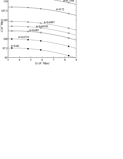
We introduce three multi-component sets, defined by different values of $h$, to establish calibration curves, which relate $h$ and the location of the BAO feature. All sets, and subsequent analysis, make use of Equation 1, and the ancillary parameter values defined in the Introduction. Since the $h$ value uniquely specifies the flat $\Lambda$CDM cosmology, we will generally refer to $h$ alone to identify a designated point. The three sets are (1) $h$=0.66 and 0.6732; (2) $h$=0.685, 0.69185, and 0.6987; and (3) $h$=0.72 and 0.7344. In all three sets the highest component differs from the lowest component by 2 per cent. Set (2) additionally has an element that differs from the lowest component by 1 per cent. The selected values span the range from Planck derived, to low-redshift derived results (Planck 2018 results VI, 2018; Riess et al., 2019). We use these sets to simulate BAO 2PCF solutions.

The matter power spectrum, $P^{\text{lin}}(k)$, used in evaluating the correlation function, is generated with the CAMB software package (Lewis, Challinor & Lasenby, 2000). A baryon-free,“no-wiggle”, spectrum (Eisenstein & Hu, 1998, 1999), $P^{\text{nw}}(k)$, is merged with $P^{\text{lin}}(k)$ to comprise a power spectrum, which suppresses higher order oscillations, thus regulating small scale non-linearities. The modified matter power spectrum, $p^{\text{mod}}(k)$, is represented as, (Percival et al., 2007),

$$P^{\text{mod}}(k)=P^{\text{nw}}(k)+[P^{\text{lin}}(k)-P^{\text{nw}}(k)]e^{-(k\Sigma_{nl})^{2}/2}.$$ (2)

The large co-moving radius of the BAO acoustic feature, $\sim$150 Mpc, leads to the feature being, for the most part, unaffected by the non-linearities initiated by the clustering of matter after recombination. However, these non-linearities, along with redshift distortions and galaxy biasing, do have some effect on the BAO correlation function peak location, $r_{p}$ (Guzik, Bernstein & Smith, 2007; Smith, Scoccimarro & Sheth, 2008; Crocce & Scoccimarro, 2008). The absolute peak location shifts by $\sim$0.5 to 1.0 percent as a result of these agencies. We focus on the ratio of fiducial and data peak positions,

$$\alpha=r_{p,\text{fid}}/r_{p},$$ (3)

rather than on the absolute scale, and disregard the large-scale perturbations in our analysis. In doing so, our ratio of fiducial and data peak positions, $r^{*}_{p,\text{fid}}/r^{*}_{p}$ differs from $\alpha$ by no more than second order terms. As long as $r^{*}_{p,\text{fid}}/r^{*}_{p}\simeq\alpha$, discounting the large-scale non-linear effects of the peak position is a valid premise. The demonstration of this result is elementary, but because it is a key assumption, we establish its validity in Appendix A. That ability to subtract out the large-scale non-linearities without deleterious effect, contrasts with the need to retain the small-scale non-linearities through use of the damping parameter, $\Sigma_{nl}$ $h^{-1}$ Mpc, in describing the matter power spectrum.

Figure 2: Functional dependence of $h$ upon $r^{*}_{p}$ for three values of $\Sigma_{\text{nl}}$. The fit line for $\Sigma_{nl}=4.76$ $h^{-1}$ Mpc, as an example, satisfies $h=0.005411r^{*}_{p}+0.1334$. The open circles are the $h$ values for the components of the three test sets found in Figure 1. Open circles are not shown for $\Sigma_{\text{nl}}$=4.76 $h^{-1}$ Mpc, due to the close proximity of the lines.

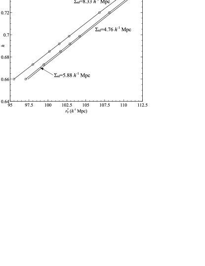
Computations have been performed at several values of $z$, dependent upon the specific circumstance. That is not a critical consideration. Though the 2PCF peak broadens with decreasing $z$, the peak position, $r_{p}^{*}$, is independent of $z$. (See, e.g., Weinberg et al. (2013), figure 11). The Fourier transform of Equation (2) (Sánchez, Baugh & Angulo, 2008) produces the correlation function in real space,

$$\xi(r)=\frac{1}{2{\pi}^{2}}\int_{0}^{\infty}dkk^{2}P^{\text{mod}}(k)j_{0}(kr)e^{-k^{2}a^{2}}.$$ (4)

Here, $a^{2}$ is a damping factor that regulates convergence at high values of $k$ where the zero order spherical Bessel function, $j_{0}(kr)$ undergoes rapid oscillation. Setting its value to 0.6 $h^{-2}~{}\text{Mpc}^{2}$, avoids interference with the determination of $r^{*}_{p}$. The 2PCF peak location, $r^{*}_{p}$, is dependent upon the value of the $P^{\text{mod}}(k)$ damping parameter, $\Sigma_{nl}$. In Figure 1, $r^{*}_{p}$ is plotted as a function of $\Sigma_{nl}$ for each component of the three test sets. Those curves are valid over a range of values, but have been generated using $\Sigma_{nl}$=3.33, 4.76, 5.88, and 8.33 $h^{-1}$ Mpc, representing approximate extreme, and median values of $\Sigma_{nl}$. The value, 8.33 $h^{-1}$ Mpc, approaches the highest damping that can be introduced before the BAO feature disappears, morphing to a plateau. Padmanabhan et al. (2012) found a value of 8.1 $h^{-1}$ Mpc, pre-recombination. The low end, 3.33 $h^{-1}$ Mpc, is comparable to the transverse component of a composite damping factor used in Ly$\alpha$ studies Kirby et al. (2013). The value 4.76 $h^{-1}$ Mpc is the inverse median of those extremes, and 5.88 $h^{-1}$ Mpc is a computation, found in Beutler et al. (2011), of a theoretical determination (Matsubara, 2008),

$$\Sigma_{nl}=\bigg{[}\frac{1}{6\pi^{2}}\int_{0}^{\infty}dkP^{lin}(k)\bigg{]}^{1/2}.$$ (5)

Figure 2 uses the same information as in Figure 1, but in this instance we plot $h$ as a function of $r^{*}_{p}$. for three values of $\Sigma_{nl}$. (The fourth value, 3.33 $h^{-1}$ Mpc, is not plotted, for clarity. As seen from Figure 1, the dependence on $\Sigma_{nl}$ flattens at the low end, leading to dense packing of the fit lines.) A linear fit is obtained for each of the values. In the following section those fits, BAO study fiducial values, and $\alpha$ (or $\alpha_{\perp}$ for anisotropic investigations) are used to evaluate $h$ and $\Omega_{m}$ for several analyzed studies.

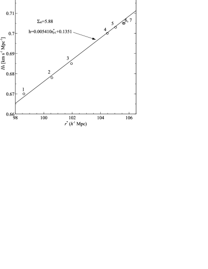
Before proceeding, we first test this procedure with known quantities. In Figure 3, the fit line for $\Sigma_{nl}=5.88h^{-1}$Mpc is plotted along with data points from three CMB studies, Calabrese et al. (2017); Planck 2015 results XIII (2016), and WMAP9, Hinshaw et al. (2013). Table 1 lists the parameter values for seven data points from those studies. Because WMAP had limited resolution in comparison with Planck, the ninth year, WMAP9, measurements are supplemented in four of the determinations with data from the high resolution Atacama Cosmology Telescope (ACT) and South Pole Telescope (SPT) missions. Two of those computations made use of both ACT and SPT, and are referred to as extended CMB, or eCMB. The test set fit line is correlated with Planck results through Equation 1. Planck data points extracted from the same data set (Planck 2015 results XIII, 2016), were analyzed by two different groups, and are included to illustrate the $\Omega_{m}$, $h$ degeneracy. The other five data points are mostly independent of Planck (Calabrese et al. (2017) incorporated the Planck 2015 results XIII (2016) reionization optical depth, $\tau$, in their analysis). The agreement in Figure 3 between the test set fit line and the data points is good enough that we emphasize that it is not a least square fit.

Figure 3: Test of fit line for $\Sigma_{nl}=5.88h^{-1}$ Mpc, $h=0.005410r^{*}_{p}+0.1351$. Values of $r^{*}_{p}$ have been computed using Table 1 data point parameter inputs , and are numbered on the figure as per the table entries.

Table 1: CMB parameter sets

$\Omega_{b}h^{2}$	$\Omega_{c}h^{2}$	$n_{s}$	$\tau$	$h$	$\Omega_{m}$	Ref.
0.02217$\pm$0.00021	0.1205$\pm$0.0021	0.9625$\pm$0.0056	0.064$\pm$0.01	0.670$\pm$0.009	0.319$\pm$0.013	(1) Calabrese et al. (2017), Planck
0.02226$\pm$0.00023	0.1186$\pm$0.0020	0.9677$\pm$0.006	0.066$\pm$0.016	0.678$\pm$0.009	0.308$\pm$0.012	(2) Planck 2015 results XIII (2016)
0.02243$\pm$0.00040	0.1156$\pm$0.0043	0.966$\pm$0.01	0.06$\pm$0.009	0.685$\pm$0.02	0.296$\pm$0.025	(3) Calabrese et al. (2017), WMAP9+ACT
0.02264$\pm$0.00050	0.1138$\pm$0.0045	0.972$\pm$0.013	0.089$\pm$0.014	0.700$\pm$2.2	0.279$\pm$0.023	(4) Hinshaw et al. (2013), WMAP9
0.02242$\pm$0.00032	0.1134$\pm$0.0036	0.9638$\pm$0.0087	0.058$\pm$0.009	0.703$\pm$0.016	0.276$\pm$0.019	(5) Calabrese et al. (2017), WMAP9+eCMB
0.02229$\pm$0.00037	0.1126$\pm$0.0035	0.9646$\pm$0.0098	0.084$\pm$0.013	0.705$\pm$1.6	0.272$\pm$0.017	(6) Hinshaw et al. (2013), WMAP9+eCMB
0.02223$\pm$0.00033	0.1126$\pm$0.0036	0.9610$\pm$0.0089	0.057$\pm$0.009	0.705$\pm$0.016	0.273$\pm$0.019	(7) Calabrese et al. (2017), WMAP9+SPT

Note. — Neutrino mass, $\Sigma m_{\nu}=0.06$ ev for data sets 1, 2, 3, 5, and 7. For data sets 4, and 6, the value is zero. $\Omega_{c}$ is the cold dark matter fraction. Calabrese et al. (2017), Planck, reference (1) refit the data from Planck 2015 results XIII (2016), Reference (2). The difference in the $\Omega_{m}$, $h$ pair values is indicative of the $\Omega_{m}$, $h$ pair degeneracy in CMB TT spectra parameter evaluations.

3 Analysis

Figure 4: Both sides of Equation 14 are plotted in (a) and (c) to assess the deviation from equality. Values of $r^{*}_{p}$, used to evaluate $\alpha$, are obtained from Figure 1, with $\Sigma_{nl}$=4.76. The normalized deviations are shown in the righthand boxes. An example of the error generated by the deviations is given in box (a), where a value of $h$=0.685 would be obtained using Equation 14 for a measurement at $z\simeq$ 0.75, rather than the correct value of $h$=0.6732. To avoid ambiguity, the value of $\alpha=0.9759$ in (a) is specifically indicated as denoting the ratio of $r^{*}_{p,\text{fid}}/r^{*}_{p}$ at $h$=0.6732

Eisenstein et al. (2005) instituted the volume averaged distance construct,

$$D_{V}(z)=\left(D_{M}^{2}(z)\frac{cz}{H(z)}\right)^{1/3},$$ (6)

where $D_{M}(z)$ is the comoving angular diameter distance, and $H(z)$ is the Hubble parameter. The function $D_{V}$(z) is designed to compensate for the distortion of radial distance in redshift space. For those analyses in which the correlation function, $\xi(r)$, is spherically averaged, and an isotropic distance scale is extracted, the BAO feature is characterized by $\alpha$, (Eq. 3).

Anderson et al. (2012); Reid et al. (2012); Sánchez et al. (2012) introduced the equation,

$$\frac{D_{V}(z)}{r_{d}}=\alpha\frac{D_{V,\text{fid}}(z)}{r_{d,\text{fid}}},$$ (7)

where $r_{d}$ is the comoving acoustic horizon at the drag epoch. That form has since been universally used for isotropic BAO studies (Padmanabhan et al., 2012; Mehta et al., 2012; Anderson et al., 2014; Kazin et al., 2014; Cuesta et al., 2016). The analogous equations used in anisotropic BAO studies are,

$$\frac{D_{M}(z)}{r_{d}}=\alpha_{\perp}\frac{D_{M,\text{fid}}(z)}{r_{d,\text{fid}}},$$ (8)

$$\frac{D_{H}(z)}{r_{d}}=\alpha_{\|}\frac{D_{H,\text{fid}}(z)}{r_{d,\text{fid}}},$$ (9)

where $D_{H}(z)=c/H(z)$.

The analysis for the anisotropic correlation function typically splits the BAO feature into two components, $r_{p\perp}$ and $r_{p\parallel}$, the transverse and radial components, respectively. As with the isotropic relationship, $\alpha=r_{p,\text{fid}}/r_{p}$, the relationships, $\alpha_{\perp}=r_{p\perp,\text{fid}}/r_{p\perp}$, and $\alpha_{\parallel}=r_{p\parallel,\text{fid}}/r_{p\parallel}$ describe the anisotropic results. Because of redshift distortion, the measured values of, $\alpha$, $\alpha_{\parallel}$ and $\alpha_{\perp}$ differ from each other. The relationships between the various dilation/contraction factors are (Cuesta et al., 2016),

$$\alpha=\alpha_{\parallel}^{1/3}\alpha_{\perp}^{2/3}$$ (10)

$$1+\epsilon=\bigg{(}\frac{\alpha_{\parallel}}{\alpha_{\perp}}\bigg{)}^{1/3},$$ (11)

where $\epsilon$ is a distortion parameter. With $\epsilon$=0, $\alpha=\alpha_{\parallel}=\alpha_{\perp}$. In calculating the fiducial value, $r_{p,\text{fid}}^{*}$, redshift distortion is not a consideration, $r_{p,\text{fid}}^{*}\equiv r_{p\perp,\text{fid}}^{*}$. Similarly, the results of Figures 1 and 2 carry over to the anisotropic analysis.

We evaluate $r_{d}$ using an expression devised by Aubourg et al. (2015) that approaches CAMB derived values to within 0.021 per cent, when values of $\omega_{cb}$ and $\omega_{b}$ are within 3$\sigma$ of the Planck derived values:

$$r_{d}\simeq\frac{55.154~{}\text{exp}[-72.3(\omega_{\nu}+0.0006)^{2}]}{\omega_{cb}^{0.25351}\omega_{b}^{0.12807}}~{}\text{Mpc},$$ (12)

where $\omega_{x}\equiv\Omega_{x}h^{2}$. The subscript, $cb$, pertains to the total mass fraction of CDM plus baryons. We assume $\Omega_{\nu}$$h^{2}$=0.00064.

Equations 7, 8, and 9 were not derived from first principles. They are algorithms that require verification. In Appendix B we demonstrate that Equations 7, and 8 provide excellent descriptions of the cosmology as $z\Rightarrow 0$. Because of redshift space distortion, we do not consider Equation 9. Equation 7 also exhibits red shift distortion. However, since the early BAO studies were all isotropic, we explore those studies in Section 3.1, and then take a second look in Subsection 3.2.2.

At the other extreme, at the drag redshift, $z_{d}\simeq$ 1060.

$$\frac{D_{M,\text{fid}}(1060)}{r_{d,\text{fid}}}\simeq\frac{D_{M}(1060)}{r_{d}}.$$ (13)

Thus, the dependence upon $\alpha_{\perp}$ in Equation 8 is not sustainable at higher values of $z$. As an illustration of the validity of Equation 13, consider the situation at the drag redshift for two values of $h$. For $h$=0.6732 $z_{d}$ =1059.82, $D_{M}(1059.82)/r_{d}$= 94.72, while for $h$=0.69185, $z_{d}$ =1059.55, $D_{M}(1059.55)/r_{d}$=94.59, a difference of $\sim$0.1 per cent. Values for $D_{M}$ are obtained from the Cosmotools online calculator. The effect of fixing $z$=1060 for both values of $h$ is inconsequential. Simulating a BAO algorithm solution, we take $h_{\text{fid}}$=0.6732, and $h$=0.69185, with $\Sigma_{nl}$=4.76, and find $\alpha_{\perp}=0.9666$, and $\alpha_{\perp}D_{M,\text{fid}}(1060)/r_{d,\text{fid}}=91.55$. That differs from $D_{M}(1060)/r_{d}$ by over 3 per cent. Our computations, in what follows, further bear out this transition from the BAO algorithms to Equation 13 with increasing $z$.

3.1 Isotropic

We rewrite Equation 7 as,

$$\alpha=\frac{r_{d,\text{fid}}D_{V}(z)}{r_{d}D_{V,\text{fid}}}.$$ (14)

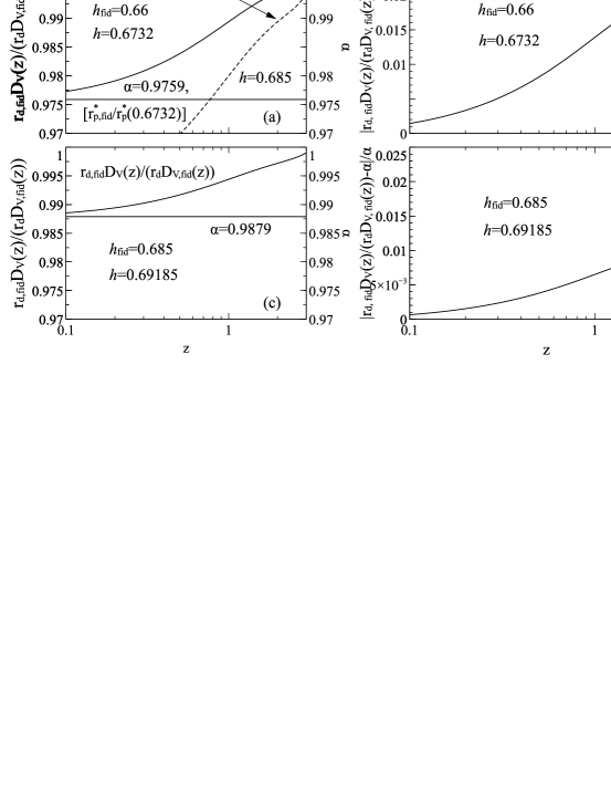
Here the left side of the equation is the measured value of $\alpha$, while the right side is the kernel of the algorithm that is being tested. We plot both sides of the equation in Figure 4a as a function of $z$. This simulation uses the two components of test set (1), $h$=0.66, and 0.6732, with 0.66 arbitrarily chosen as the fiducial value. $D_{V}(z)$ and $D_{V,\text{fid}}(z)$ are evaluated using Equation 6. As throughout this manuscript, calculations are performed for a flat cosmology, with $w=-1$, and therefore,

$$H(z)=H_{0}[\Omega_{m}(1+z)^{3}+1-\Omega_{m}]^{1/2}~{}\text{km}~{}\text{s}^{-1}\text{Mpc}^{-1}.$$ (15)

Figure 4a shows distinct deviation between the two sides of Equation 14 with increasing redshift. The difference between $\alpha$ and $r_{d,\text{fid}}D_{V}(z)/(r_{d}D_{V,\text{fid}}(z))$ normalized to $\alpha$ is depicted in Figure 4b, and is about 1 per cent at $z\simeq$ 0.75. Since $\alpha$ would be the measured quantity, and the fiducial values are a given, the deduced value of $h$ from Figure 4a at $z\simeq$ 0.75, as indicated on the figure, and when using Equation 14, is $h\simeq 0.685$, rather than the actual value of $h=0.6732$. We find similar results for the $h$ pairs for the other two test sets, where $h_{\text{fid}}$ and $h$ differ by two per cent. In Figure 4c and d we plot the pair from test set (2) in which $h_{\text{fid}}$ and $h$ differ by 1 per cent, and, as to be expected, find a substantial reduction in the deviation, a one per cent deviation, being found here at $z\simeq 3$.

In Figures 4a and 4c note that the right hand side of Equation 14 has made significant progress towards unity at the coordinate maximum of $z$=3, far from the drag value of $\sim 1060$. That follows since, at $z\sim 3$, for the flat $\Lambda$CDM cosmologies considered here, the age of the Universe was $\sim$ 2.2 Gyr, and thus the transition of the right side of Equation 14 from near equality with $\alpha$ to near equality with unity, as dictated by Equation 13, occurs at a much lower redshift value than might at first be anticipated.

BAO 2PCF results from 2005 to date can be characterized as first generation, in that the standard deviations are typically several per cent. The Alam et al. (2017) combined measurements, presented in several papers based on the SDSS-III Baryon Oscillation Spectroscopic Survey (BOSS), represent the highest attained first generation precision, of $\sim$ 1 per cent. For surveys conducted at low values of redshift, such as Beutler et al. (2011) at $z=0.106$, and Ross et al. (2015) at $z=0.15$ the Equation 7 algorithm is a good fit. Beyond those two low redshift figures, BAO galactic studies span a range of 0.32 $\eqslantless$ $z$ $\eqslantless$ 0.73. We will not systematically appraise those studies. However, we do examine two isotropic studies, Cuesta et al. (2016), because of its 1 per cent precision, and Ata et al. (2018), because of its high redshift. Cuesta et al. (2016), like Alam et al. (2017), was based on the Data Release 12 (DR12) of the SDSS BOSS program, and summary figure 13 of Alam et al. (2017) indicates that it is a good representation of those studies. Measurements were conducted at effective redshifts $z$=0.32, and 0.57. We address the $z$=0.57 results. Ata et al. (2018) evaluated measurements on a population of quasars centered at a redshift of 1.52.

In Figure 5 we reproduce the fit lines of Figure 2. That is not strictly correct for application to specific BAO studies, since they include the large-scale perturbations that we have neglected. Including those perturbations would slightly shift the fit lines, however, as in Appendix A, the difference between the two results is of second order. By expressing $r^{*}_{p}$ as $r^{*}_{p,\text{fid}}/\alpha$, the value of $h$ is derived with known quantities. Thus, for $\Sigma_{\text{nl}}=4.76$ $h^{-1}$ Mpc,

$$h=0.005411r^{*}_{p,\text{fid}}\big{/}\alpha+0.1334,$$ (16)

and for $\Sigma_{\text{nl}}=5.88$ $h^{-1}$ Mpc,

$$h=0.005410r^{*}_{p,\text{fid}}\big{/}\alpha+0.1351.$$ (17)

The fit line equation for $\Sigma_{\text{nl}}=8.33$ $h^{-1}$ Mpc is,

$$h=0.005285r^{*}_{p,\text{fid}}\big{/}\alpha+0.1554.$$ (18)

Table 2: Fiducial parameter sets for BAO studies discussed in this paper

$\Omega_{b}h^{2}$	$n_{s}$	$\sigma_{8}$	$h$	$\Omega_{m}$	Ref.
0.02247	0.97	0.8	0.7	0.29	Cuesta et al. (2016)
0.022	0.97	0.8	0.676	0.31	Ata et al. (2018)
0.02222	0.9655	0.830	0.6731	0.3147	Bautista et al. (2017)
0.0227	0.97	0.8	0.7	0.27	Delubac et al. (2015)

Note. — The neutrino mass, $\Sigma m_{\nu}=0.06$ ev for all data sets, with the exception of Cuesta et al. (2016), where it is set equal to zero. des Bourboux et al. (2017); de Sainte Agathe et al. (2019); Blomqvist et al. (2019) use the same fiducial values as Bautista et al. (2017), and Font-Ribera, et al. (2014) use the same values as Delubac et al. (2015).

All fiducial values for studies discussed herein can be found in Table 2. For Cuesta et al. (2016) $\Sigma_{\text{nl}}=5.0$ $h^{-1}$ Mpc (see Vargas-Magaña, et al. (2018), for which our value of 4.76 is adequate. We depict $r^{*}_{p,\text{fid}}$=103.9 $h^{-1}$ Mpc on the plot. Note that it does not fall on the fit line, since the fiducial parameters do not satisfy the $h$, $\Omega_{m}$ near degeneracy condition of Equation 1. We assume that the derived data do satisfy the near degeneracy condition. The study measured $\alpha$=1.0093$\pm$0.0097, which from Equation 16 leads to $h$=0.6904$\pm$0.0058. While the fiducial value of $\Sigma_{nl,\text{fid}}$ is a given, we do not know the actual damping parameter value. Cuesta et al. (2016) performed their analysis before and after implementing the reconstruction technique initiated by Eisenstein et al. (2007). That method employs the galaxy density data to compute the velocity field and then, effectively, runs the clock backwards, reversing the inflowing mass. We use the Cuesta et al. (2016) post-reconstruction results, in which case we can dismiss the likelihood of higher damping levels (Padmanabhan et al., 2012). Thus the narrow damping parameter uncertainty indicated in the plot.

Figure 5: The fit lines of Figure 2 are reproduced here, and the loci of the Cuesta et al. (2016), and Ata et al. (2018) $h$ limits indicated, as determined from Equations 16 and 17. The vertical lines delimit the extent of the damping parameter uncertainty.

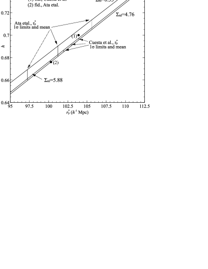
Ata et al. (2018) assign $\Sigma_{\text{nl}}=6.0$ $h^{-1}$ Mpc, which is adequately approximated by our $\Sigma_{\text{nl}}=5.88$ $h^{-1}$ Mpc. They found $\alpha$=0.991$\pm$0.037. Their fiducial parameters return $r^{*}_{p,\text{fid}}$=100.4 $h^{-1}$ Mpc, which, from Equation 17, leads to $h$=0.6832$\pm$0.022. Because of the low density of quasars, Ata et al. (2018) were not able to perform reconstruction. Therefore in Figure 5 we depict a large damping parameter uncertainty, extending from $\Sigma_{\text{nl}}=8.33$ $h^{-1}$ Mpc down to the region where the fit lines coalesce. At the mean value of $\alpha$, with regard to Equation 14, the normalized deviation is $\mid$$\alpha$ - $r_{d,\text{fid}}D_{V}(z)/(r_{d}D_{V,\text{fid}}(z))$$\mid$$\big{/}$$\alpha$=0.008. Considering the $\alpha$ standard deviation of $\sim$3.7 per cent, the bias introduced by using Equation 14 is not appreciable.

Though Cuesta et al. (2016) achieved a precision where deviations could be of import, the relatively low redshift of $z$=0.57, and a value of $\alpha$ close to unity, minimized the negative influence. Because of the predominantly large variances of first generation isotropic BAO studies, the deviations from equality in Equation 14 do not, in general, adversely affect the results. The proviso to that conclusion is that the deviations are not errors to be added in quadrature, but rather, with respect to Equation 14, are unwanted biases that are directly, and misleadingly, added to flat $\Lambda$CDM consistent results. We return to the subject of isotropic BAO studies in Subsection 3.2.2.

3.2 Anisotropic

Figure 6: Both sides of Equation 21 are plotted in the upper and lower panels for Bautista et al. (2017) at $z$=2.33, and for des Bourboux et al. (2017) at $z$=2.4, respectively, to assess the deviation from equality. The standard deviation bars for $\alpha_{\perp}$ are shifted to the left for clarity.

Anisotropic determinations (Xu et al., 2013; Kazin et al., 2013; Anderson et al., 2014, 2014b; Cuesta et al., 2016) have been facilitated as spectroscopic galaxy surveys have increased in size. They provide more detail than the isotropic average, and when taken together with reconstruction (Xu et al., 2013) contribute to a more nuanced understanding of BAO conditions. Although reconstruction significantly ameliorates the effects of redshift distortion (Weinberg et al., 2013), those effects are not completely eliminated. The most direct measure of the BAO feature is provided by $\alpha_{\perp}$. Redshift distortion is not a factor here, and $r_{p\perp}$ is a direct measure in real space as well as in redshift space. For that reason, in what follows, we concentrate on that transverse component.

3.2.1 Ly$\alpha$ forest anisotropic studies

Figure 7: Both sides of Equation 21 are plotted for the weighted average $\alpha_{\perp}=0.943\pm 0.030$ values of the Delubac et al. (2015); Font-Ribera, et al. (2014) Ly$\alpha$ forest studies. The fiducial values listed in Table 2 yield $r_{p,\text{fid}}^{*}$=105.7, and the flat $\Lambda$CDM solution is $h=0.739\pm 0.020$. The mean normalized discrepancy is $\mid$$\alpha_{\perp}$-$r_{d,\text{fid}}D_{M}(z)/(r_{d}D_{M,\text{fid}}(z))$$\mid$/$\alpha_{\perp}$$\simeq$0.033. Apparent values to satisfy Equation 21 are $h=0.788\pm 0.048$, and $\Omega_{m}=0.1969^{+0.040}_{-0.032}$. The standard deviation bars for $\alpha_{\perp}$ are shifted to the left for clarity.

Table 3: Comparison of anisotropic and isotropic computations of $\Omega_{m}$ and $h$

Ref.		$\alpha_{\perp}$	$\Omega_{m}(\alpha_{\perp})$	$\alpha$	$\Omega_{m}(\alpha)$
Survey	Effec. $z$	$\alpha_{\parallel}$	$h(\alpha_{\perp})$	$\rho_{\alpha_{\perp}\alpha_{\parallel}}$	$h(\alpha$)
Cuesta et al. (2016)	0.57	1.0368$\pm$0.0142	0.312$\pm$0.011	1.0051$\pm$0.0098	0.290$\pm$0.070
BOSS DR12		0.9446$\pm$0.0324	0.676$\pm$0.008	-0.5671	0.693$\pm$0.006
Blomqvist et al. (2019)	2.35	0.923$\pm$0.046	$0.258^{+0.034}_{-0.031}$	0.971$\pm$0.028	0.293$\pm$0.022
eBOSS DR14		1.076$\pm$0.042	$0.720^{+0.032}_{-0.030}$	-0.44	$0.690^{+0.018}_{-0.017}$
de Sainte Agathe et al. (2019)	2.34	0.953$\pm$0.048	$0.280^{+0.038}_{-0.034}$	0.979$\pm$0.03	0.299$\pm$0.024
eBOSS DR14		1.033$\pm$0.034	$0.701^{+0.032}_{-0.029}$	-0.34	$0.686^{+0.019}_{-0.018}$

Note. — Isotropic ratio, $\alpha$, is computed using Equation 10. Fiducial parameters for Cuesta et al. (2016) are the same as for the isotropic analysis. Fiducial values for de Sainte Agathe et al. (2019) and Blomqvist et al. (2019) are identical to those of Bautista et al. (2017) and des Bourboux et al. (2017). For Cuesta et al. (2016), the computed value from Equation 10 compares favorably with their isotropic measurement of $\alpha$=1.0093$\pm$0.0097.

Ly$\alpha$ forest BAO measurements are undertaken at redshifts, $z>2$, and are therefore of specific interest in this study. The auto-correlation Ly$\alpha$ forest analysis of Bautista et al. (2017) and the cross-correlation study of des Bourboux et al. (2017) cover the same segments of sky, but their $\alpha_{\perp}$, $\alpha_{\parallel}$, pairs are largely uncorrelated (des Bourboux et al., 2017).

The Ly$\alpha$ forest computations model the damping parameter as (Kirby et al., 2013),

$$\Sigma^{2}(\mu_{k})=\mu_{k}^{2}\Sigma_{\parallel}^{2}+(1-\mu_{k}^{2})\Sigma_{\perp}^{2}.$$ (19)

Here, $\mu_{k}$ is the cosine of the angle between the radial direction and the line joining two tracers ‘of the large-scale distribution of matter in redshift space’. $\Sigma_{\parallel}=6.41$ $h^{-1}$ Mpc, and $\Sigma_{\perp}=3.26$ $h^{-1}$ Mpc. We use our $\Sigma_{nl}$ value of 3.33 $h^{-1}$ Mpc, which is close to the $\Sigma_{\perp}$ value of 3.26 $h^{-1}$ Mpc. The fit line for $\Sigma_{\text{nl}}=3.33$ $h^{-1}$ Mpc is,

$$h=0.005431r^{*}_{p\perp,\text{fid}}\big{/}\alpha_{\perp}+0.1304$$ (20)

From the fiducial values we find, $r^{*}_{p,\text{fid}}$=100.13 $h^{-1}$ Mpc. Analogous to Equation 14, we rewrite Equation 8 as,

$$\alpha_{\perp}=\frac{r_{d,\text{fid}}D_{M}(z)}{r_{d}D_{M,\text{fid}}},$$ (21)

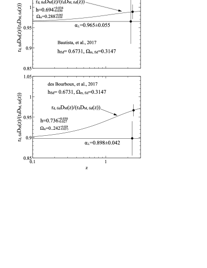
and plot both sides of the equation in Figure 6. Although each study is represented by one point on the plot, Bautista et al. (2017), at $z$=2.33 in the top panel, and des Bourboux et al. (2017), at $z$=2.4 in the lower panel, we have plotted the mean values of $\alpha_{\perp}$ and $r_{d,\text{fid}}D_{M}(z)/(r_{d}D_{M,\text{fid}}(z))$ over a range of redshifts, $0.1<z<3.0$ to give an indication of the deviation from equality as $z$ increases. For Bautista et al. (2017) we find $h=0.694^{+0.036}_{-0.032}$, and for des Bourboux et al. (2017), $h=0.736^{+0.031}_{-0.029}$. These values differ significantly from the fiducial values, selected by the authors to coincide with Planck 2015 results XIII (2016). The deviations of Equation 21 from equality would move the apparent values even further from the Planck likelihood.

The Bautista et al. (2017) and des Bourboux et al. (2017) measurements have been updated by de Sainte Agathe et al. (2019) and Blomqvist et al. (2019) using the same fiducial parameters. Blomqvist et al. (2019) provides a combined fit value for both studies of $\alpha_{\perp}=0.942^{+0.032}_{-0.030}$, from which we find $h=0.708\pm 0.02$.

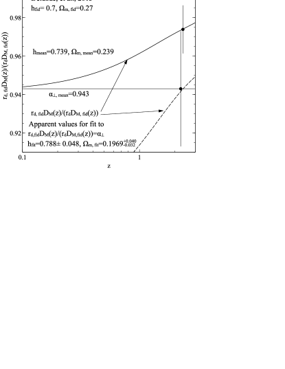
Aubourg et al. (2015); Addison et al. (2018); Planck 2018 results VI (2018) have all noted the discrepancy between the Ly$\alpha$ forest BAO measurements and the Planck evaluation, with the former consistently finding higher values of $h$. We have also found that to be true, but additionally the Aubourg et al. (2015); Addison et al. (2018); Planck 2018 results VI (2018) investigations used the BAO Equations 8, and 9. Therefore, we expect that they would find an even larger disparity. In addition to performing joint fits between BAO and Planck data, Addison et al. (2018) also considered constraints from the BAO scale alone. For that undertaking they combined earlier Ly$\alpha$ forest studies, Delubac et al. (2015); Font-Ribera, et al. (2014). In Figure 7 we plot our analysis of the weighted average of those two studies. The data point is at $z$=2.35. We find $h=0.739\pm 0.020$. The apparent value of $h$ that satisfies Equation 21 is $0.788\pm 0.048$, with $\Omega_{m}=0.1969^{+0.040}_{-0.030}$. By employing Equation 21, Addison et al. (2018), figure 3, elicited a similar result, providing a clear-cut example of the misleading nature of Equations 8 and 21 at higher values of $z$.

3.2.2 Assessment of isotropic measurements

Separate from our analysis of the applicability of the BAO equations, we turn back to consideration of isotropic results in light of what is observed in anisotropic measurements. Table 3 lists $\alpha_{\perp}$, $\alpha$, and respective derived values of $\Omega_{m}$ and $h$ for the most recent Ly$\alpha$ forest studies, de Sainte Agathe et al. (2019) and Blomqvist et al. (2019), plus the anisotropic results of Cuesta et al. (2016), earlier considered regarding isotropic outcomes. The isotropic ratio, $\alpha$, is computed using Equation 10. As previously noted, $\alpha_{\perp}$ provides the most reliable measure, in that it is free of the effects of redshift distortion. For each of the three studies, there is a pronounced difference between the $h$ and $\Omega_{m}$ results as determined by $\alpha_{\perp}$, versus those determined by $\alpha$. Because of this significant dissimilarity, we question the viability of using isotropic study results for cosmological parameter assessments. Specifically, Beutler et al. (2011) and Ross et al. (2015) have both been used in the Aubourg et al. (2015); Addison et al. (2018); Planck 2018 results VI (2018) investigations. Because of their low redshifts, we concluded that there was no problem with using Equation 7 to describe these results. However, with increased precision, and the ability to perform anisotropic measurements, use of these earlier isotropic results is unwarranted.

4 Conclusions

The BAO Equations 7 and 8 are algorithms, which, as demonstrated in Appendix B, are accurate when $z\Rightarrow 0$, and, as established in the text, are adequate at low values of $z$, in particular for the early BAO studies, with high variances. (Because of redshift distortion, the third algorithm of the set, Equation 9 was not considered.) We have focused on the transition of the quantity, $r_{d,\text{fid}}D_{M}(z)/(r_{d}D_{M,\text{fid}}(z))$ from $\alpha_{\perp}$ as $z\Rightarrow 0$, to $\sim$ unity as $z\Rightarrow z_{d}\simeq 1060$. At the lower limit, the transverse anisotropic BAO algorithm provides an excellent fit. However, with increasing $z$ that equation deviates from an accurate description. Figures 4, 6 and 7 indicate how rapidly that transition takes place. At $z\sim 3$, when the age of the Universe was $\sim$2.2 Gyr, it has moved substantially towards completion.

The isotropic solution includes the radial $\alpha_{\parallel}$ component, which in turn incorporates redshift distortion. The transverse component, $\alpha_{\perp}$, provides a determination in both redshift and real space, and is free of redshift distortion. Comparisons of $h$ and $\Omega_{m}$ values derived using this measure, as opposed to values derived with the isotropic measure, $\alpha$, show differences of several percent. We conclude that given the clarity of the transverse anisotropic measurements, studies, such as those of Aubourg et al. (2015); Addison et al. (2018); Planck 2018 results VI (2018), which evaluate cosmological parameters would better reflect reality by omission of the isotropic results.

At the higher redshifts of Ly$\alpha$ studies, $z\simeq$ 2.35, the anisotropic BAO algorithms give decidedly misleading results. We have replicated an example from Addison et al. (2018), in which use of the BAO algorithms points to a mean value of $\Omega_{m}\sim$ 0.197, while the flat $\Lambda$CDM analysis yields a mean value closer to 0.239.

The next generation of BAO studies, (Vargas-Magaña, et al., 2019; Euclid Collaboration, 2019; Doré, et al., 2019), will improve precision to $\sim$ 0.3 percent. Under those circumstances, even uncertainties between the fiducial damping parameter, $\Sigma_{nl,\text{fid}}$ and the actual damping parameter, $\Sigma_{nl}$, can introduce errors comparable to that precision. We have demonstrated that the BAO algorithms are not suitable for that tightened state of affairs. On the other hand, an analysis assuming a flat, $w=-1$, $\Lambda$CDM cosmology, such as we have done herein, accords a straightforward procedure for preliminary appraisals.

Appendix A Validity of assumption, $r_{p,\text{fid}}^{*}/r_{p}^{*}$$\simeq\alpha$

We write,

$$\alpha=\frac{r_{p,\text{fid}}}{r_{p}}=\frac{r_{p,\text{fid}}^{*}+\Delta_{\text{fid}}}{r_{p}^{*}+\Delta}.$$ (A1)

Here, $\Delta$ and $\Delta_{\text{fid}}$ represent the shifts introduced by large-scale non-linearities. Let $\alpha=1+\gamma$. The ratio $r_{p,\text{fid}}^{*}/r_{p}^{*}$ is then,

$$\frac{r_{p,\text{fid}}^{*}}{r_{p}^{*}}=\alpha+\frac{\gamma\Delta+(\Delta-\Delta_{\text{fid}})}{r_{p}^{*}},$$ (A2)

and the approximation is demonstrated, since $\mid$$\gamma$$\mid$ is generally $<$0.05, $\mid$$\Delta$$\mid$/$r_{p}^{*}$ is of the order 0.005–0.01, and the ($\Delta-\Delta_{\text{fid}}$)/$r_{p}^{*}$ term is of the same magnitude as $\gamma\Delta$/$r_{p}^{*}$.

Appendix B BAO equations behavior as $z$ $\Rightarrow{0}$

As $z\Rightarrow 0$, the ratios $D_{M}/D_{M,\text{fid}}$ and $D_{V}/D_{V,\text{fid}}$ both $\Rightarrow$ ${h_{\text{fid}}}/h$, the familiar short range measure. Focusing on Equation 21, we rewrite it as,

$$\alpha_{\perp}=\frac{r_{d,\text{fid}}}{r_{d}}\frac{h_{\text{fid}}}{h},$$ (B1)

and derive expressions for each side of the equation. For $\alpha_{\perp}$, from the various fit line formulas, Equations 16, 17, 18, and 20, we obtain,

$$\alpha_{\perp}=\frac{h_{\text{fid}}}{h}\frac{(1-C/h_{\text{fid}})}{(1-C/h)}.$$ (B2)

Here C is the constant in the fit formulas, e.g., 0.1334 in Equation 16. We reformulate that expression using the following approximation,

$$\alpha_{\perp}\simeq\frac{h_{\text{fid}}}{h}\big{[}1+C/h_{\text{fid}}(1+C/h+C^{2}/h^{2}+C^{3}/h^{3})\frac{\Delta h}{h}\big{]},$$ (B3)

where $\Delta h=h_{\text{fid}}-h$.

From Equation 12, $r_{d,\text{fid}}/r_{d}$ takes the form,

$$\frac{r_{d,\text{fid}}}{r_{d}}\simeq\frac{(\Omega_{cb}h^{2})^{0.25351}(\Omega_{b}h^{2})^{0.12807}}{(\Omega_{cb,\text{fid}}h_{\text{fid}}^{2})^{0.25351}(\Omega_{b,\text{fid}}h_{\text{fid}}^{2})^{0.12807}},$$ (B4)

Making use of Equation 1 we find,

$$\frac{r_{d,\text{fid}}}{r_{d}}\simeq\frac{(\Omega_{b}h^{2})^{0.12807}}{(\Omega_{b,\text{fid}}h_{\text{fid}}^{2})^{0.12807}}[1+0.00168\Delta h]\bigg{(}\frac{h_{\text{fid}}}{h}\bigg{)}^{0.25351},$$ (B5)

The factor, $[1+0.00168\Delta h]$, stems from subtracting the neutrino mass fraction, $\Omega_{\nu}h^{2}=0.00064$ from $\Omega_{m}h^{2}$ to obtain $\Omega_{cb}h^{2}$. That factor can be dropped, with little loss of accuracy, leading to the expression,

$$\frac{r_{d,\text{fid}}}{r_{d}}\simeq\frac{(\Omega_{b}h^{2})^{0.12807}}{(\Omega_{b,\text{fid}}h_{\text{fid}}^{2})^{0.12807}}\bigg{(}\frac{h_{\text{fid}}}{h}\bigg{)}^{0.25351}.$$ (B6)

Within a range of values, such as found in Table 1, the ratio, $(\Omega_{b}h^{2})^{0.12807}/(\Omega_{b,\text{fid}}h_{\text{fid}}^{2})^{0.12807}$, differs from unity, at most, by less than three tenths of a per cent, and therefore for this exercise we also drop that term

The right side of Equation B1 is now expressed as,

$$\frac{r_{d,\text{fid}}}{r_{d}}\frac{h_{\text{fid}}}{h}\simeq\bigg{(}\frac{h_{\text{fid}}}{h}\bigg{)}^{1.25351}$$ (B7)

Placing the equation in the same format as Equation B3, we have,

$$\frac{r_{d,\text{fid}}}{r_{d}}\frac{h_{\text{fid}}}{h}\simeq\frac{h_{\text{fid}}}{h}(1+0.25351\frac{\Delta h}{h}),$$ (B8)

Though it is not obvious that Equations B2/B3 and B7/B8 give very similar results, a couple of examples should suffice as a demonstration. First consider the test set $h_{\text{fid}}=0.66$, $h=0.6732$, and Equation 16, $\Sigma_{nl}=4.76$ $h^{-1}$ Mpc, C=0.1334. For those values, Equation B2 gives $\alpha_{\perp}=0.9755$, while Equation  B7 also yields $r_{d,\text{fid}}h_{\text{fid}}/(r_{d}h)=0.9755$. At the other extreme of the range for $h$, and taking a value of $\alpha_{\perp}$ further removed from unity, we select from the test sets, $h_{\text{fid}}=0.6987$, and $h=0.7344$, with $\Sigma_{nl}=5.88$ $h^{-1}$ Mpc, C=0.1351. For these conditions we find, $\alpha_{\perp}=0.9404$, and $r_{d,\text{fid}}h_{\text{fid}}/(r_{d}h)=0.9394$. For $\Sigma_{nl}=8.33$ $h^{-1}$ Mpc, $\alpha_{\perp}=0.9383$. Thus, throughout the range of relevant values for $h$ and $\Sigma_{nl}$, $r_{d,\text{fid}}h_{\text{fid}})/(r_{d}h)$ and $\alpha_{\perp}$ converge towards a common value.

This demonstration is not satisfactory from the perspective of lacking a clear analytical limit. That problem stems from the empirical nature of both Equation 12, defining $r_{d}$, and of the fit lines that define $\alpha_{\perp}$. We cannot overcome that shortcoming in this presentation, but the approximations of Equations B3 and B8 perhaps make the demonstration more palatable. They take the same form, the difference being in the terms multiplying $\Delta h/h$. The demonstration works because those factors are small, affecting the third and fourth significant figures. As a result, some degree of inequality can be tolerated, while still bringing about convergence.

References

- Addison et al. (2013) Addison, G. E., Hinshaw, G., Halpern, M., 2013, MNRAS, 436, 1674
- Addison et al. (2018) Addison, G. E., Watts, D. J., Bennett, C. L., et. al., 2018, ApJ, 853, A119
- Alam et al. (2017) Alam, S., Ata, M., Bailey, S., et al., 2017, MNRAS. 470, 2617
- Anderson et al. (2012) Anderson, L., Aubourg, E., Bailey, S., et al., 2012, MNRAS, 427, 3435
- Anderson et al. (2014) Anderson, L., Aubourg, E., Bailey, S., et al., 2014, MNRAS, 441, 24
- Anderson et al. (2014b) Anderson, L., Aubourg, E., Bailey, S., et al. 2014b MNRAS439, 83
- Ata et al. (2018) Ata,, M., Baumgarten, F., Bautista, J., et al. 2018, MNRAS, 473, 4773
- Aubourg et al. (2015) Aubourg, E., Bailey, S., Bautista, J. E., et al., 2015, Phys. Rev. D, 92,123516
- Bautista et al. (2017) Bautista, J. E., Busca, N. G., Guy, J., et al., 2017, A&A, 603, A12
- Betoule et al. (2014) Betoule, M., Kessler, R., Guy, J., et al., 2014, A&A, 568, A22
- Beutler et al. (2011) Beutler, F., Blake, C., Colless, M., et al., 2011, MNRAS, 416, 3017
- Blomqvist et al. (2019) Blomqvist, M., Bourboux, H. M., Busca, N. G., et al., 2019, A&A, 629, A86
- Calabrese et al. (2017) Calabrese, E., Hložek, R.A., Bond, J. R., et al. 2017, Phys. Rev. D, 95, 063525
- Cole et al. (2005) Cole, S., Percival, W. J., Peacock, J. A., et al., 2005, MNRAS, 362, 505
- Cooke et al. (2018) Cooke, R. J., Pettini, M., & Steidel, C. C,, 2018, ApJ, 855, 102
- Crocce & Scoccimarro (2008) Crocce, M., Scoccimarro, R., 2008, Phys. Rev. D, 77, 023533
- Cuesta et al. (2016) Cuesta, A.J., Vargas-Magana, M., Beutler, F., et al., 2016, MNRAS, 457, 1770
- Delubac et al. (2015) Delubac, T., Bautista, J. E., Rich, J., et al., 2015, A&A, 574, A59
- de Sainte Agathe et al. (2019) de Sainte Agathe, V., Balland, C., du mas des Bourboux, H., et al. 2019, A&A, 629, A85
- des Bourboux et al. (2017) du mas des Bourboux, H., Le Goff, J.-M., Blomqvist, M., et al., 2017, A&A, 608, A130
- Doré, et al. (2019) Doré O., et al., 2019 preprint (arXiv:1904.01174)
- Eisenstein & Hu (1998) Eisenstein, D. J., Hu, W., 1998, ApJ, 496, 605
- Eisenstein & Hu (1999) Eisenstein, D. J., Hu, W., 1999, ApJ, 511, 5
- Eisenstein et al. (2005) Eisenstein, D. J., Zehavi, I., Hogg, D. W., et al., 2005, ApJ, 633, 560
- Eisenstein et al. (2007) Eisenstein, D. J., Seo, H-J., Sirko, E., Spergel, D. N., 2007, ApJ, 664, 675
- Euclid Collaboration (2019) Euclid preparation: VII, 2019, preprint, (arXiv:1910.09273)
- Font-Ribera, et al. (2014) Font-Ribera, A., Kirby, D., Busca, N., et al., 2014, J. Cosmology Astropart. Phys, 5, 027
- Guzik et al. (2007) Guzik, J., Bernstein, G., Smith, R. E., 2007, MNRAS, 375, 1329
- Hinshaw et al. (2013) Hinshaw, G., Larson, D., Komatsu, E., et al., 2013, ApJS, 208, 19
- Kirby et al. (2013) Kirby, D., Margala, D., Slosar, A., et al., 2013, J. Cosmology Astropart. Phys, 03, 024
- Komatsu et al. (2011) Komatsu, E., Dunkley, J., Nolta, M. R., et al., 2011, ApJS, 192,18
- Kazin et al. (2013) Kazin, E. A., Sánchez, A. G., Cuesta, A. J., et al. 2013, MNRAS, 435, 64
- Kazin et al. (2014) Kazin, E. A., Koda, J., Blake, C., et al., 2014, MNRAS, 441, 3524
- Lewis, Challinor & Lasenby (2000) Lewis, A., Challinor, A., Lasenby, A., 2000, ApJ, 538, 473
- Matsubara (2008) Matsubara, T., 2008, Phys. Rev. D, 77, 063530
- Mehta et al. (2012) Mehta, K. T., Cuesta, A. J., Xu, X., Eisenstein, D. J., Padmanabhan, N., 2012, MNRAS, 427, 2168
- Padmanabhan et al. (2012) Padmanabhan, N., Xu, X., Eisenstein, D. J., et al., 2012, MNRAS, 427, 2132
- Percival et al. (2002) Percival, W. J., Sutherland, W., Peacock, J. A., et al. 2002, MNRAS, 337, 1068
- Percival et al. (2007) Percival, W. J., Nichol, R. C., Eisenstein, D. J., et al., 2007, ApJ, 657, 645
- Planck 2013 results XVI (2014) Planck 2013 results XVI, 2014, A&A, 571, A16
- Planck 2015 results XIII (2016) Planck 2015 results XIII, 2016, A&A, 594, A13
- Planck 2018 results VI (2018) Planck 2018 results VI, 2018, [arXiv:1807.06209]
- Reid et al. (2012) Reid, B., Samushia, L., White, M., et al., 2012, MNRAS, 426, 2719
- Riess et al. (2019) Riess, A. G., Castertano, S., Yuan, W., et al., 2019, ApJ, 876, 85
- Ross et al. (2015) Ross, A. J., Samushia, L., Howlett, C., et al., MNRAS, 449, 835
- Sánchez, Baugh & Angulo (2008) Sánchez, A. G., Baugh, C. M., Angulo, R., 2008, MNRAS, 390, 1470
- Sánchez et al. (2012) Sánchez, A. G., Scóccola, C. G., Ross, A. J., et al. 2012, MNRAS, 425, 415
- Simard et al. (2018) Simard, G., Omori, Y., Aylor, K., et al. 2018, ApJ, 860, 137
- Smith et al. (2008) Smith, R. E., Scoccimarro, R., Sheth, R. K.,2008, Phys. Rev. D, 77, 043525
- Spergel et al. (2007) Spergel, D. N., Bean, R., Doré, O., et al., 2007, ApJ, 170, 377
- Vargas-Magaña, et al. (2018) Vargas-Magaña, M., Ho, S., Cuesta, A. J., et al., 2018, MNRAS, 477, 1153
- Vargas-Magaña, et al. (2019) Vargas-Magaña, M., Brooks, D. D., Levi, M. M., Tarle, G. G., on behalf of DESI collaboration, 2019, preprint (arXiv:1901.01581)
- Weinberg et al. (2013) Weinberg, D. H., Mortonson, M. J., Eisenstein, D. J., et. al., 2013,Phys. Rep.530, 2, 87
- Xu et al. (2013) Xu, X., Cuesta, A. J., Padmanabhan, N., Eisenstein, D. J., McBride, C. K. 2013, MNRAS, 431, 2834