A quantum heat engine with coupled superconducting resonators

Abstract

We propose a quantum heat engine composed of two superconducting transmission line resonators interacting with each other via an optomechanical-like coupling. One resonator is periodically excited by a thermal pump. The incoherently driven resonator induces coherent oscillations in the other one due to the coupling. A limit cycle, indicating finite power output, emerges in the thermodynamical phase space. The system implements an all-electrical analog of a photonic piston. Instead of mechanical motion, the power output is obtained as a coherent electrical charging in our case. We explore the differences between the quantum and classical descriptions of our system by solving the quantum master equation and classical Langevin equations. Specifically, we calculate the mean number of excitations, second-order coherence, as well as the entropy, temperature, power and mean energy to reveal the signatures of quantum behavior in the statistical and thermodynamic properties of the system. We find evidence of a quantum enhancement in the power output of the engine at low temperatures.

I Introduction

Heat engines with quantum working substances, so-called quantum heat engines (QHEs), have attracted much attention recently Kieu ; Quan et al. (2007, 2005); Abah et al. (2012); Bergenfeldt et al. (2014); Henrich et al. (2007); Uzdin and Kosloff (2014); Scully et al. (2003, 2011); Scully (2010); Brunner et al. (2012); Manzano et al. (2016); Song et al. (2016); Altintas et al. (2015); Ivanchenko (2015); Altintas et al. (2014); Dağ et al. (2016); Türkpençe and Müstecaplıoğlu (2016); Hardal and Müstecaplıoğlu (2015); Campisi and Fazio (2016); Kosloff and Levy (2014); Tonner and Mahler (2005); Anders and Giovannetti (2013); Zhang et al. (2014a, b); Zhang and Zhang (2017); Mari et al. (2015); Gelbwaser-Klimovsky and Kurizki (2015); Roßnagel et al. (2014); Allahverdyan and Nieuwenhuizen (2000); Korzekwa et al. (2016); Perarnau-Llobet et al. (2015); Plastina et al. (2014); Campo et al. (2014); Roulet et al. (2017); Hofer et al. (2016a, 2017a, b); Karimi and Pekola (2016). The steam driven mechanical piston is an archetype of classical heat engines. Quantum analogs of piston engines have been proposed using optomechanical models, where steam is replaced by a photonic gas Mari et al. (2015); Gelbwaser-Klimovsky and Kurizki (2015); Roßnagel et al. (2014); Zhang et al. (2014a, b); Zhang and Zhang (2017). A single-atom piston engine described by an effective optomechanical model has been demonstrated in the classical regime very recently Roßnagel et al. (2016). The benefits of “quantumness” Uzdin et al. (2015); Mukherjee et al. (2016) as well as the quantum-to-classical transition Quan et al. (2006) in heat engines are fundamental problems in the emerging field of quantum thermodynamics. We propose a quantum heat engine composed of a pair of superconducting resonators interacting via an effective optomechanical coupling Johansson et al. (2014). It offers an on-chip circuit analog of a piston engine and could be used to explore fundamental quantum properties in heat engines.

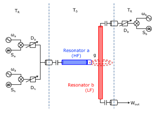
We specifically consider a system of two coupled superconducting resonators Johansson et al. (2014), as an alternative embodiment of the piston cycle used in the single-atom heat engine Roßnagel et al. (2016). In our case, which is shown in Fig. 1, the resonator modes play the role of vibrational modes of the trapped atom. One of the resonators is periodically driven by a quasi-thermal pump and interacts with the other resonator through an effective optomechanical coupling Johansson et al. (2014). The emergence of coherence in one mode by incoherent excitation of the other is a typical feature of quantum piston engines exploiting optomechanical coupling Mari et al. (2015). We investigate the quantum statistics of the resonator modes by calculating the mean number dynamics, occupation probability distributions, and second-order correlation functions. We verify that the incoherently driven mode remains thermal while the other becomes almost coherent. In addition, thermodynamic properties of the system are examined by calculating the mean energy versus effective electrical length of the driven resonator and the temperature versus entropy diagrams of the engine. We identify that the system undergoes an Otto engine cycle. We find that, after a transient regime, a limit cycle emerges in the thermodynamical phase space, indicating finite power output, at the same time that the driven mode induces steady coherent oscillations in the other mode.

Figure 1: (Colour online) Circuit diagram of the quantum heat engine composed of two superconducting microwave resonators interacting via an effective optomechanical like coupling with strength $g$. Resonators indicated by “a” and “b”, have high frequency (HF) and low frequency (LF) modes with $\omega_{a}\gg\omega_{b}$. HF mode is periodically driven by a variable amplitude attenuation ($D_{h}$) white noise source ($S_{h}$), corresponding to an effective hot bath at $T_{h}$. The resonators are on a chip at a background temperature $T_{0}$. External noise drives are at room temperature $T_{R}$. Both the LF and HF resonators are subject to additional quasi-thermal sources implemented by amplitude controlled ($D_{a},D_{b})$ white noise drives $(S_{a},S_{b})$, which are constantly applied to the corresponding resonators.

Further, we compare the quantum mechanical results with those obtained from the classical Langevin equations of motion. We find significant qualitative and quantitative differences between the classical and quantum descriptions of the system. In particular, the power output from the quantum piston engine is greater than that of the classical one at low temperatures. We argue that the quantum enhancement in power output can be observed in superconducting resonators. We explain the effect by identifying the type of quantum correlation behind the power output as the so-called signal-meter correlation Holland et al. (1990); Mancini et al. (1997) and compare it with the classical correlations. It is not a universal fact that quantum correlations can always increase the power output of a piston engine. Recent studies reported exactly the opposite conclusions where quantum fluctuations cause less power output in a rotor type piston engine Roulet et al. (2017).

This paper is organized as follows. In Section II, we introduce the quantum optomechanical engine model based upon coupled superconducting transmission line resonators. In Section III, we describe our numerical methods and present the results of quantum dynamical simulations. The corresponding classical engine model is introduced in Sec. IV and the results of the classical Langevin equation simulations are given in Sec. V. These results are compared to the quantum description. In Sec. VI, we discuss the quantum character of the model system in terms of the quantum coherence and correlations. We conclude in Section VII.

II The Quantum Model

Our model system consists of two superconducting transmission line resonators on a chip, held at temperature $T_{0}$, as shown in Fig. 1. A resonator, indicated by “a” in the figure, is terminated by a SQUID, which collects the flux generated by the other resonator, indicated by “b”, so that an effective optomechanical-like coupling, denoted by $g$, between the resonators can be engineered Johansson et al. (2014). We assume resonator “a” with frequency $\omega_{a}$ is shorter than resonator “b” with frequency $\omega_{b}$ such that $\omega_{a}\gg\omega_{b}$. The high frequency (HF) and low frequency (LF) modes of resonator “a” and resonator “b” can be considered as analogs of the optical and mechanical modes of an optomechanical system, respectively. The effective optomechanical-like coupling between the resonators is expressed as (we take $\hbar=1$) Johansson et al. (2014)

$$\hat{H}_{\text{sys}}=\omega_{a}\hat{a}^{\dagger}\hat{a}+\omega_{\text{b}}\hat{b}^{\dagger}b-g\hat{a}^{\dagger}\hat{a}(\hat{b}+\hat{b}^{\dagger}),$$ (1)

where $\hat{a}$ ($\hat{a}^{\dagger}$) and $\hat{b}$ ($\hat{b}^{\dagger}$) are the annihilation (creation) operators for the HF and LF modes, respectively.

In addition to the cold environment at $T_{0}$, we assume three microwave white noise drives are applied to the resonators. These drives are produced by external sources at room temperature, $T_{R}$. We consider two continuously applied noises with power spectral densities $S_{a}$ and $S_{b}$ on the resonators a and b, respectively. Their amplitudes can be controlled by variable amplitude attenuators $D_{a}$ and $D_{b}$. The HF resonator is subject to another amplitude controlled ($D_{h}$) and periodic white noise source with a power spectral density $S_{h}$. The power spectral densities are assumed to be narrow band, centered at the corresponding resonator frequencies $\omega_{a}$ and $\omega_{b}$, but much wider than the bandwidth of the HF resonator. Accordingly, each externally applied noise source approximates a one-dimensional black body (thermal) spectrum Fink et al. (2010) at effective temperatures that can be determined from the Planck distribution functions, (we take $k_{B}=1$),

$$\bar{n}_{a} = \frac{1}{\exp{(\omega_{a}/T_{a})}-1},$$ (2)

$$\bar{n}_{b} = \frac{1}{\exp{(\omega_{b}/T_{b})}-1},$$ (3)

$$\bar{n}_{h} = \frac{1}{\exp{(\omega_{a}/T_{h})}-1},$$ (4)

where $T_{h},T_{b}$ and $T_{a}$ are the effective temperatures corresponding to the periodic drive, continuous drive on the HF resonator, and the continuous drive on the LF resonator, respectively. We assume the periodic drive is used to engineer an effective hot bath such that $T_{h}>T_{a},T_{b}$. The mean number of excitations in the cold baths are denoted by $\bar{n}_{a}$ and $\bar{n}_{b}$, for the HF and LF modes, respectively. The mean number of excitations in the periodically modulated hot reservoir is denoted by $\bar{n}_{\text{h}}$. The one dimensional Planck’s law gives the power spectral densities as $S_{x}=\omega_{x}\bar{n}_{x}$ with $x=a,b,h$. We consider engineering the two additional cold baths to get more flexibility to reach desired steady states in the engine operation, which may not be achieved in the case of a common single environment at $T_{0}$. A similar strategy was employed for the case of the single-atom piston engine by using an additional cooling laser Roßnagel et al. (2016).

The dynamics of the density matrix $\hat{\rho}$ of the resonator pair can be determined by a master equation Fink et al. (2010),

$$\dot{\hat{\rho}} = -i[\hat{H}_{\text{sys}},\hat{\rho}]$$

$$+ \kappa_{a}(\bar{n}_{a}+1)D[\hat{a}]+\kappa_{a}\bar{n}_{a}D[\hat{a}^{\dagger}]$$

$$+ \kappa_{b}(\bar{n}_{b}+1)D[\hat{b}]+\kappa_{b}\bar{n}_{b}D[\hat{b}^{\dagger}]$$

$$+ \kappa_{\text{h}}(t)(\bar{n}_{\text{h}}+1)D[\hat{a}]+\kappa_{h}(t)\bar{n}_{\text{h}}D[\hat{a}^{\dagger}]$$

$$+ \kappa_{0}^{a}(\bar{n}_{0}^{a}+1)D[\hat{a}]+\kappa_{0}^{a}\bar{n}_{0}^{a}D[\hat{a}^{\dagger}]$$

$$+ \kappa_{0}^{b}(\bar{n}_{0}^{b}+1)D[\hat{b}]+\kappa_{0}^{b}\bar{n}_{0}^{b}D[\hat{b}^{\dagger}]$$

Here, $D[\hat{\alpha}]:=(1/2)(2\hat{\alpha}\hat{\rho}\hat{\alpha}^{\dagger}-\hat{\alpha}^{\dagger}\hat{\alpha}\hat{\rho}-\hat{\rho}\hat{\alpha}^{\dagger}\hat{\alpha})$ refers to the Lindblad dissipator superoperators with $\hat{\alpha}=\hat{a},\hat{b}$. $\kappa_{a}$ and $\kappa_{b}$ are effective coupling constants of the HF and LF modes with their local cold baths, respectively. The coupling coefficient of the HF mode with the effective hot bath is denoted by $\kappa_{\text{h}}(t)$, which has a periodic time dependence. Small background field excitations are denoted by $n_{0}^{a}$ and $n_{0}^{b}$ in the corresponding terms of the master equation describing the coupling of the environment at $T_{0}$ with the HF and LF resonators at rates $\kappa_{0}^{a}$ and $\kappa_{0}^{a}$, respectively.

We assume a special case that each local cold bath, engineered with the quasi-thermal noise drive, has the same excitation number so that we can introduce $\bar{n}_{c}:=\bar{n}_{a}=\bar{n}_{b}$, which is possible for $T_{a}/T_{b}=\omega_{a}/\omega_{b}$. Accordingly we have $T_{a}\gg T_{b}$. It may be worth emphasizing that the local temperatures are “effective” and can be high (e.g. $100$ K or more) because very little of the noise power is absorbed by the resonators Fink et al. (2010).

The master equation we consider assumes the usual Born-Markov approximations under the weak coupling with the noise sources. Moreover, as we use local effective reservoirs in the dissipators, the dynamics may not be consistent with the second law of thermodynamics at all parameter regimes Levy and Kosloff (2014). It is usually assumed that such a local master equation should be reliable when the coupling between the subsystems (here the HF and LF resonators) is sufficiently weak Hofer et al. (2017b); González et al. (2017). To determine the validity regime for our case, we also used a “global” master equation (see Appendix A) derived for arbitrary optomechanical coupling strengths Hu et al. (2015) to compare the results with the “local” master equation. We found that both local and global master equation results agree well in the range under consideration $g\leq\omega_{b}$. The regime of $g=\omega_{b}$ is not exactly the ultrastrong coupling regime of optomechanics, as we have large $\kappa_{a}>g$. In the temperature regimes we consider, the excitation of the HF resonator is weak $\langle n_{a}\rangle<1$. We explore a regime of single “photon” optomechanics which is not well charted.

III Quantum Dynamics of the Engine

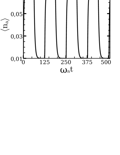
In our simulations we use dimensionless parameters by scaling $\omega_{b}/2\pi=500$ MHz, $g/2\pi=500$ MHz, $\kappa_{h}/2\pi=\kappa_{a}/2\pi=2$ GHz and $\kappa_{b}/2\pi=50$ MHz by $\omega_{a}/2\pi=10$ GHz. The temporal profile of the incoherent drive acting on the HF mode is taken as a square wave $\kappa_{h}(t):=\kappa_{h}s(t)$. The square wave $s(t)=1$ and $s(t)=0$ for the heating and cooling stages, respectively. Each stage takes the same time of $\pi/\omega_{b}$. In units of $1/\omega_{a}$ the cycle duration is then $t_{\text{cycle}}=(2\pi)20$ (cf. Fig. 2).

The mean number of excitations in the effective baths are taken to be $\bar{n}_{a}=\bar{n}_{b}:=\bar{n}_{\text{c}}=0.01$ and $\bar{n}_{h}>0.1$, for which our simulations yield limit cycles for the engine operation at steady state. The corresponding effective temperatures become $T_{a}\sim 104$ mK and $T_{b}\sim 5$ mK. A typical environment temperature for the superconducting resonators is $T_{0}\sim 20$ mK. Accordingly the hierarchy of temperatures associated with the engineered environments for the resonators becomes $T_{h}>T_{a}>T_{0}>T_{b}$. The temperature ranges of $T_{h}>T_{a}>T_{0}$ have been successfully produced experimentally for a single superconducting resonator using the noise drive method Fink et al. (2010). The range of $T_{0}>T_{b}$ can be engineered using proposals for optomechanical schemes Teufel et al. . The HF resonator mode is effectively heated to $T_{h}$ when the external periodic noise pulse is on, and when the pulse is off it effectively cools to $T_{a}$. The LF resonator is always coupled to an effective cold bath.

The quantum dynamics of the coupled resonators subject to such effective heating and cooling stages is investigated by solving Eq. (II) using QuTiP Johansson et al. (2013). We neglect the last four terms associated with the background environment in Eq. (II) by assuming $\kappa_{a}\gg\kappa_{0}^{a}$ and $\kappa_{0}^{b}\bar{n}_{0}^{b}>\kappa_{b}\bar{n}_{b}$. After an intake stage, where the resonators are at their respective initial states, repeated action of the the heating and cooling stages will lead the system into a limit cycle that can be considered as a heat engine cycle with a net power output.

The system is assumed to be in an initial state $\hat{\rho}(0)=\hat{\rho}_{a}(0)\otimes\hat{\rho}_{b}(0)$, where

$$\hat{\rho}_{a}(0) = \frac{1}{\text{Tr}e^{-\omega_{a}\hat{a}^{\dagger}\hat{a}/T_{a}}}e^{-\omega_{a}\hat{a}^{\dagger}\hat{a}/T_{a}},$$ (6)

$$\hat{\rho}_{b}(0) = \frac{1}{\text{Tr}e^{-\omega_{b}\hat{b}^{\dagger}\hat{b}/T_{b}}}e^{-\omega_{b}\hat{b}^{\dagger}\hat{b}/T_{b}},$$ (7)

are the initial density matrix operators of the HF and LF modes, respectively. Initial occupations of the modes then are $\bar{n}_{c}$ since $\langle\hat{n}_{x}\rangle(0)=\langle\hat{x}^{\dagger}\hat{x}\rangle(0)=Tr(\hat{\rho}(0)\hat{x}^{\dagger}\hat{x})=\bar{n}_{c}=0.01$, with $x=a,b$.

Figure 2: (Colour online) Dynamics of the mean number of excitations (a) $\langle\hat{n}_{a}\rangle$ and (b) $\langle\hat{n}_{b}\rangle$ in the HF and LF modes, respectively, for $\bar{n}_{\text{h}}=0.125$ (black-solid), $\bar{n}_{\text{h}}=0.325$ (red-dashed), $\bar{n}_{\text{h}}=0.525$ (green-dotted) and $\bar{n}_{\text{h}}=0.725$ (blue-dot-dashed).(c) Dynamics of the LF field coherence is characterized by $\Re(\langle b\rangle)$, where $\Re\equiv Re$ denotes the real part. Time is dimensionless and scaled with the HF mode frequency $\omega_{a}$. All the other parameters are as explained in the text.

III.1 Quantum piston in phase space

The heating and cooling stages in the engine operation of the coupled resonator system can be visualized by examining the dynamics of the mean excitation numbers $\langle\hat{n}_{x}\rangle=\langle\hat{x}^{\dagger}\hat{x}\rangle=Tr(\hat{\rho}(t)\hat{x}^{\dagger}\hat{x})$, with $x=a,b$, which are shown in Fig. 2. The dynamics of $\langle\hat{n}_{a}\rangle$ is shown in Fig. 2 for $\bar{n}_{\text{h}}=0.125$. The heating pulse duration is taken to be longer than the thermalization time of the HF resonator. When the heating pulse is applied, the HF mode reaches a steady state at $\langle\hat{n}_{a}\rangle_{\text{ss}}\sim 0.0675$, which is the same as the analytical result $\langle\hat{n}_{a}\rangle_{\text{ss}}=(\bar{n}_{c}+\bar{n}_{\text{h}})/2$ (see the Appendix B). After the heating pulse, the excitation number first rapidly drops and then slowly cools back to the initial value. Analytical expressions can be approximately given as

$$\langle\hat{n}_{a}\rangle=\begin{cases}\frac{\bar{n}_{a}+\bar{n}_{h}}{2}-\frac{\bar{n}_{h}-\bar{n}_{a}}{2}e^{-(\kappa_{a}+\kappa_{h})t},&0\leq t<\frac{\pi}{\omega_{b}};\\ \bar{n}_{a}+\frac{\bar{n}_{h}-\bar{n}_{a}}{2}e^{-\kappa_{a}(t-\pi/\omega_{b})},&\frac{\pi}{\omega_{b}}\leq t<\frac{2\pi}{\omega_{b}},\end{cases}$$ (8)

which is repeated indefinitely.

Figure 3: (Colour online) (a)-(d) The occupation probability (OP) with respect to occupation number of the Fock states $n_{\text{fock}}$ of the LF resonator mode at $\omega_{\text{a}}t=5000$ for $\bar{n}_{\text{h}}=0.125$ (a), $\bar{n}_{\text{h}}=0.325$ (b), $\bar{n}_{\text{h}}=0.525$ (c) and $\bar{n}_{\text{h}}=0.725$ (d). All the other parameters are as explained in the text.

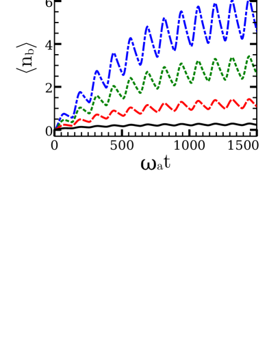
The dynamics of the mean excitations of the LF mode $\langle\hat{n}_{b}\rangle$ are shown in Fig. 2, which reaches a steady state with coherent oscillations in the long time limit. Both the time average $\langle\hat{n}_{b}\rangle$ value and the amplitude of the oscillations are larger for larger $\bar{n}_{\text{h}}$; while the frequency of oscillations remains the same. The heating pulse duration is only long enough to thermalize the HF resonator, while the LF resonator is unable to equilibrate in a pulse period. The evolution of the LF resonator will start from a different initial condition for every pulse action. This “memory” effect leads to a higher time average $\langle\hat{n}_{b}\rangle$ value than the one found under continuous drive (cf. Appendix). In addition, correlations between the HF and LF resonator modes contribute to to the dynamics of the LF mode excitations. We will explore the physical mechanisms behind the dynamics of $\langle n_{b}\rangle$ in more detail in Sec. VI.

Fig. 2 plots the “electrical displacement” of the LF mode, $\Re(\langle\hat{b}\rangle)=q/2$, where $q=\langle\hat{q}\rangle=\langle\hat{b}+\hat{b}^{\dagger}\rangle$, showing coherent oscillations in the steady state. The notation $\Re(\cdot)$ stands for the real part. In contrast to the dynamics of $\langle n_{b}\rangle$, $q$ has identical classical and quantum dynamics. Its equation of motion (see Appendix) is that of a periodically driven damped oscillator, which is given by

$$\ddot{q}+\kappa_{b}\dot{q}+\omega^{2}q=2\omega_{b}g\langle n_{a}(t)\rangle,$$ (9)

where $\omega^{2}=\omega_{b}^{2}+\kappa_{b}^{2}/4$ and the dots over $q$ indicate time derivatives. This equation can be interpreted in terms of an effective series RLC circuit. The cold environment of the LF resonator acts as the resistive element dampening the LC oscillations. In the standard way, the natural frequency $\omega_{b}$ of the LC oscillations is further renormalized by the damping rate $\kappa_{b}$. The HF resonator provides the input voltage which sustains the oscillations. Despite the thermal nature of the HF resonator, it drives the RLC circuit into coherent oscillations because the drive only depends on $\langle n_{a}\rangle$, which is alternating between high and low values periodically. We note that while $q$ is not vanishing in the steady state, the electrical momentum $p=\langle\hat{p}\rangle=i\langle(\hat{b}^{\dagger}-\hat{b})\rangle$ becomes approximately zero (It is exactly zero according to the global master equation as can be seen in the Appendix B).

The LF oscillator is in the weak damping regime ($\kappa_{b}<\omega_{b}$). The formal solution of Eq. (9) is given by

$$q(t)=2g\int_{0}^{t}\text{d}\,t^{\prime}\langle n_{a}(t^{\prime})\rangle e^{-\frac{\kappa_{b}}{2}(t-t^{\prime})}\sin{(\omega_{b}(t-t^{\prime}))}.$$ (10)

The periodic nature of $\langle n_{a}(t^{\prime})\rangle$ leads to an intuitive understanding of the emergence of a coherent steady state in $q(t)$. Harmonics of $\langle n_{a}(t^{\prime})\rangle$ are given by the frequencies $\omega_{k}=k\omega_{b}$ where $k$ is an integer. According to Eq. (10) the maximum overlap or the resonance would occur for the first harmonic $k=1$. Besides, the higher harmonics would have relatively smaller significance as their amplitudes get smaller with $k$. Accordingly, steady state oscillations in $q(t)$ are dominated by the single frequency $\omega_{b}$. The time average value of $q$, as well as the amplitude of oscillations, increase linearly with $\bar{n}_{h}$. In terms of our physical parameters, the approximate analytical solution is found to be

$$q=\frac{\bar{n}_{h}+3\bar{n}_{c}}{2}+\frac{20(\bar{n}_{h}-\bar{n}_{c})}{\pi}\sin\left(\omega_{b}t-1.55\right).$$ (11)

A more general solution is given in the Appendix C.

Figure 4: (Colour online) Phase portrait $\langle q_{b}\rangle-\langle p_{b}\rangle$ showing the dynamics of the LF mode for $\bar{n}_{\text{h}}=0.125$. All the other parameters are as explained in the text.

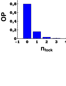
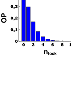
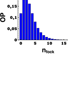
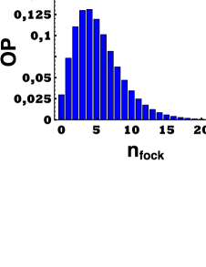
We further visualize the coherence in the steady state of the LF mode by investigating the probability distribution $P(n):=\langle n|\rho_{b}(t)|n\rangle$, where $\rho_{b}(t)=\text{Tr}_{a}[\rho(t)]$ is the reduced density matrix of the LF mode, in Fig. 3. As we increase $\bar{n}_{\text{h}}$ from $\bar{n}_{\text{h}}=0.125$ to $\bar{n}_{\text{h}}=0.725$, the the probability distribution changes from a thermal distribution to a coherent distribution, as shown in Figs. 3-3.

In Fig. 4, we plot the dynamics of the mean values of the field quadratures $q_{b}:=\langle\hat{q}_{\textbf{b}}\rangle:=q/\sqrt{2}$ and $p_{b}:=\langle\hat{p}_{\textbf{b}}\rangle:=p/\sqrt{2}$, where $p=\langle\hat{p}\rangle:=i\langle(\hat{b}^{\dagger}-\hat{b})\rangle$, with respect to each other. The resulting phase diagram is that of a periodically driven damped displaced harmonic oscillator, where the slight shift of the center of the limit cycle from the origin is the signature of the coherent displacement induced by the thermal drive. The HF mode reaches steady state within a single thermal noise pulse duration as shown in Fig. 2. The action of the thermal noise pulse on the HF mode is translated to the LF mode by the optomechanical coupling. According to Fig. 2, the LF mode can reach an oscillatory steady state after the action of a several noise pulses. As the LF mode lags behind the HF mode, there will be a transient regime before a limit cycle is established, as we see in In Fig. 4. While a limit cycle emerges for our model, we note that the existence of a stable limit cycle after transients is in general model and initial condition dependent Feldmann and Kosloff (2004). Within the approximation of $\langle\hat{n}_{a}\rangle$ as a square wave drive, we find an expression for the limit cycle (see Appendix C)

$$(p_{b}-p_{b0})^{2}+(q_{b}-q_{b0})^{2}=R^{2},$$ (12)

where

$$R = \frac{4}{\pi}\frac{\sqrt{2}\omega_{b}g}{\sqrt{\kappa_{b}^{2}\left(\omega_{b}^{2}+\frac{\kappa_{b}^{2}}{16}\right)}}\left(\frac{\bar{n}_{h}-\bar{n}_{c}}{4}\right),$$ (13)

$$q_{b0} = \frac{2\omega_{b}g}{\sqrt{2}\omega^{2}}\left(\frac{\bar{n}_{h}+3\bar{n}_{c}}{4}\right),$$ (14)

and $p_{b0}\approx 0$.

Figure 5: (Colour online) Time dependence of the zero-time delay second order correlation function $g^{(2)}(0)$ of the LF mode for $\bar{n}_{\text{h}}=0.125$ (black-solid), $\bar{n}_{\text{h}}=0.325$ (red-dashed), $\bar{n}_{\text{h}}=0.525$ (green-dotted) and $\bar{n}_{\text{h}}=0.725$ (blue-dot-dashed). The inset is the magnification of $g^{(2)}(0)$ up to $10\omega_{a}t$. Time is dimensionless and scaled with the HF mode frequency $\omega_{a}$. All the other parameters are as explained in the text.

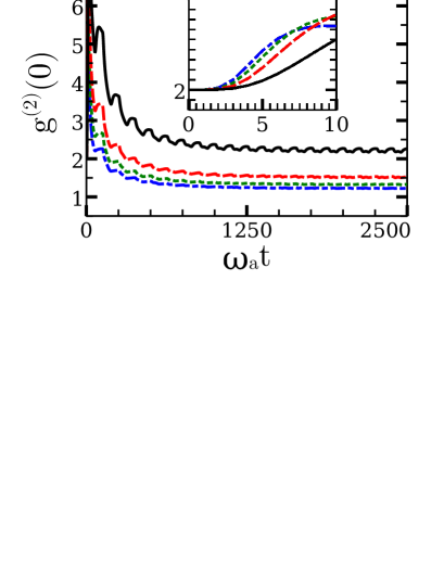
The effect of coherence in the LF mode state can be further revealed by calculating the zero-time delay second order correlation function $g^{(2)}(0):=\langle\hat{b}^{\dagger}\hat{b}^{\dagger}\hat{b}\hat{b}\rangle/\langle\hat{n}_{b}\rangle^{2}$, of the LF mode. Fig. 5 shows the time dependence of $g^{(2)}(0)$ of the LF mode for the same $\bar{n}_{\text{h}}$ values as in Fig. 2. Initially, $g^{(2)}(0)=2$ for all cases as the LF mode starts in a thermal state. $g^{(2)}(0)$ decrease as the LF mode gains partial coherence in time. At higher $\bar{n}_{\text{h}}$, the steady state value of $g^{(2)}(0)$ gets closer to the coherent state value $g^{(2)}(0)=1$. While perfect coherence is not achieved within the range of values of $\bar{n}_{\text{h}}$ considered, a slow convergence to coherent state statistics can be seen in Fig. 5. We note that the second-order coherence function can be measured in circuit QED systems using various techniques such as by linear detectors da Silva et al. (2010).

III.2 Semi-classical Engine cycle

Figure 6: (Colour online) (a) Dependence of the effective internal energy of the HF resonator $U_{a}=\omega_{\text{eff}}\langle\hat{n}_{a}\rangle$ on the effective HF mode frequency $\omega_{\text{eff}}=\omega_{a}-g(\langle\hat{b}\rangle+\langle\hat{b}^{\dagger}\rangle)$ for $\bar{n}_{\text{h}}=0.125$ in the steady state. (b) The plot shows $\ln{(U_{a})}$ in order to emphasize that the temperature in the lower branch (D^′ to A) is increasing. The direction of the engine cycle in the steady state is indicated by the red arrows. The points A, B, B^′, C, D, and D^′ are used in the text to describe the thermodynamic processes in the cycle. We use the frequency of the HF resonator, $\omega_{a}$, to scale our parameters. All the other parameters are as explained in the text.

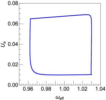
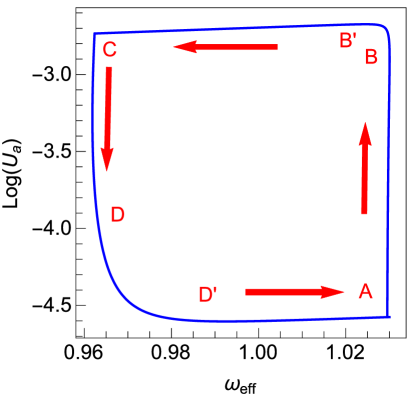
In order to describe the engine cycle, we introduce an effective HF mode frequency $\omega_{\text{eff}}:=\omega_{a}-gq$, which can be interpreted as the change in the frequency associated with the variations in the electrical length of the HF resonator. Accordingly, the effective mean energy of the working fluid can be taken to be $U_{a}=\omega_{\text{eff}}\langle\hat{n}_{a}\rangle$. This semiclassical factorization ignores the correlations between $\hat{n}_{a}$ and $\hat{q}$. When we calculate $U_{a}$ without the factorization assumption, we find qualitatively the same cycle pictures and the work output is negligibly enhanced. For the moment, we consider the semiclassical explanation of the engine cycle and discuss the effect of quantum correlations separately in the later sections.

Figure 7: (Colour online) Steady state dependence of the entropy $S(\rho_{a})$ on the effective HF mode frequency $\omega_{\text{eff}}=\omega_{a}-g(\langle\hat{b}\rangle+\langle\hat{b}^{\dagger}\rangle)$ for $\bar{n}_{\text{h}}=0.125$. We use the frequency of the HF resonator $\omega_{a}$ to scale our parameters. All the other parameters are as explained in the text.

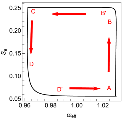
In Fig. 6, we plot the dependence of $U_{a}$ on $\omega_{\text{eff}}$ in the steady state at $\bar{n}_{\text{h}}=0.125$, for the same set of parameters used in earlier figures. We plot $\ln{(U_{a})}$ in order to emphasize that the temperature in the lower branch (D^′ to A) is increasing. A four stage engine cycle can be identified in this picture.

The first stage is indicated by the arrow from point A to B in Fig. 6 at $\omega_{\text{eff}}\sim 1.03$ and corresponds to an isochoric heating of the HF resonator by the incoming heat pulse. The electrical length $1/\omega_{\text{eff}}$ remains constant while the incoherent energy is received from the external noise pulse. The coherence of the LF mode cannot follow the thermalization of the HF mode as fast (cf. Fig. 2) so that the “piston”, or the LF mode quadrature, remains at rest in the phase space. There is a transitional stage from B to B^′ which cannot be identified with the standard thermodynamical processes.

Figure 8: (Colour online) $T-S$ diagram of the HF mode for $\bar{n}_{\text{h}}=0.125$. We use the frequency of the HF resonator, $\omega_{a}$, to scale our parameters. All the other parameters are as explained in the text.

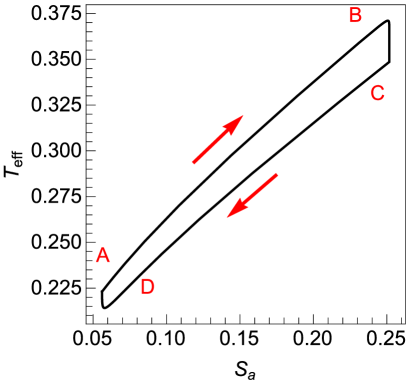
The second stage, from B^′ to C, is adiabatic expansion of the HF resonator, where $\omega_{\text{eff}}$ decreases to $\sim 0.96$ and hence the electrical length of the HF resonator increases. The entropy of the HF resonator field can be calculated by

$$S_{a}=(1+\langle\hat{n}_{a}\rangle)\ln{(1+\langle\hat{n}_{a})}-\langle\hat{n}_{a}\rangle\ln{(\langle\hat{n}_{a})},$$ (15)

which remains constant in this stage as shown in Fig. 7. The heating pulse is still active, but the HF mode is in thermal equilibrium and working on the LF mode. The coherence in the LF mode builds up in this stage as the “piston” shifts in the phase space, converting heat to potential energy to be harvested.

The third stage is isochoric cooling that happens from C to D at $\omega_{\text{eff}}\sim 0.96$, following the rapid decrease of the population of the HF mode when the heating pulse is turned off (cf. Fig. 2). There is another transitional stage from D to D^′. The final stage from D^′ to A closes the cycle. It corresponds to an adiabatic compression (cf. Fig. 7) where $\omega_{\text{eff}}$ increases to $\sim 1.03$. The sign change in the coherence of the LF mode (cf. Fig. 2) leads to an increasing $\omega_{\text{eff}}$ (decreasing electrical length) so that the “piston” moves back to its original location in the phase space and the cycle is complete.

III.3 Performance of the engine

Our 4-stage engine description, other than the transitional stages, can be considered as an Otto cycle. The effects of the transitional stages do not strongly influence the temperature-entropy (T-S) diagram plotted in Fig. 8, which closely resembles that of an Otto engine. Here we introduced an effective temperature given by

$$T_{\text{eff}}=\omega_{\text{eff}}/\ln{(1+1/\langle\hat{n}_{a}\rangle)}.$$ (16)

The T-S diagram in Fig. 8, which follows a narrow cycle, is of a similar form to that obtained experimentally for the single-atom heat engine Roßnagel et al. (2016) and for a nanomechanical Otto engine driven by a squeezed reservoir to operate with an efficiency beyond the classical Carnot limit Klaers et al. (2017).

The area of such diagrams can be considered as the potential work output from the working fluid. By approximating the diagram in Fig. 8 by a trapezoid, we can estimate the net work by $W_{a}\sim 3.5\times 10^{-3}\hbar\omega_{a}\sim 2.3\times 10^{-26}$ joules. Dividing by the cycle time, which is the heating pulse period $2\pi/\omega_{b}=2$ ns, we find the power from the working fluid as $P_{a}\sim 1.15\times 10^{-17}$ Watts. The heat intake of the HF resonator can also be determined from the diagram and we find $Q_{\text{in}}\sim 0.06\hbar\omega_{a}$ which yields an efficiency of $\eta=W_{a}/Q_{\text{in}}\sim 0.06\%$. Similar values can be consistently found from the cycle in $\langle\hat{n}_{a}\rangle$-$\omega_{\text{eff}}$ diagram, which is similar to Fig. 6. Approximating the cycle by a rectangular path, we can verify that $W_{a}\sim\hbar(n_{H}-n_{L})(\omega_{H}-\omega_{L})$, where $n_{H}\sim 0.0675$ and $n_{L}=0.01$ (cf. Fig. 2) are the maximum and minimum $\langle\hat{n}_{a}\rangle$, respectively. Similarly, $\omega_{H}\sim 1.04$ and $\omega_{L}\sim 0.96$ (see e.g. Fig. 7) are the maximum and minimum of $\omega_{\text{eff}}$, respectively. The heat intake in this case can be written as $Q_{\text{in}}\sim\hbar\omega_{H}(n_{H}-n_{L})$. Hence, the efficiency becomes that of an Otto engine $\eta=1-\omega_{L}/\omega_{H}\sim 0.08\%$ These values increase with $\bar{n}_{h}$. For example, at $\bar{n}_{h}=1$, we get $\eta\sim 0.27\%$, $P\sim 2.64\times 10^{-16}$ J/s, and $W\sim 5.28\times 10^{-25}$ J. We cannot increase $\bar{n}_{h}$ indefinitely however. Optomechanical model requires relatively small oscillations such that $\omega_{a}>g|q|$ at all times. This limits our considerations to a regime $\bar{n}_{h}<3.25$.

Figure 9: (Colour online) The maximum power (in units of $\kappa_{b}\hbar\omega_{a}$) with respect to average number of excitations $\bar{n}_{\text{h}}$ in the effective hot bath. The black solid, red dotted, and blue dashed curves indicate the results of the semiclassical, classical, and quantum calculations. All the other parameters are as explained in the text.

Figure 10: (Colour online) Behavior of the relative difference in the dissipative power with respect to average number of excitations $\bar{n}_{H}$ in the hot bath. Red dashed and blue solid curves indicate $(P_{q}-P_{c})/P_{q}$ and $(P_{q}-P_{sc})/P_{q}$ where $P_{q},P_{c}$, and $P_{sc}$ are calculated by quantum, classical, and semiclassical methods, respectively. Power is dimensionless and scaled with $\kappa_{b}\hbar\omega_{a}$. All the other parameters are as explained in the text.

For practical purposes, a figure of merit called the dissipative power is also considered to estimate the performance of such piston engines, which is given by Mari et al. (2015)

$$P = -{\text{Tr}}\{\omega_{b}\hat{n}_{b}\kappa_{b}[(\bar{n}_{b}+1)D[\hat{b}]+\bar{n}_{b}D[\hat{b}^{\dagger}]]\}$$ (17)

$$= \omega_{b}\kappa_{b}\big{(}\langle\hat{n}_{b}\rangle-\bar{n}_{\text{c}}\big{)}.$$ (18)

It is non-zero when the LF resonator mode is not in equilibrium with the environment. It has the same qualitative behaviour with the mean number of excitations in the LF mode by definition and hence is oscillatory around a mean value (cf. Fig. 2). In steady state it has a highly intuitive relation to the power output of the Otto cycle of the HF resonator. In order to see this we note that $\langle\hat{n}_{a}\rangle=0$ in the adiabatic branches of the cycle so that the mean energy $U_{a}=\omega_{a}\langle\hat{n}_{a}\rangle-g\langle\hat{n}_{a}\hat{q}\rangle$ varies as

$$\frac{dU_{a}}{dt}=-g\omega_{b}\langle\hat{n}_{a}\hat{p}\rangle,$$ (19)

which is identical with $-P$ in the steady state (cf. Appendix B). Here, we did not employ the factorization assumption and have used the unitary part of the equation of motion for the $\langle\hat{n}_{a}\hat{q}\rangle$, which can be obtained from the equations of motion in Appendix A. As the mean energy is determined by the usual force (pressure) times distance type expression, the associated power is also expressed by the typical force times velocity type formula. The difference from the classical mechanics expressions is that quantum or classical statistical correlations can contribute to the expectation values. $P$ is called the dissipative power because it is approximately the same as the heat current from the LF resonator to its thermal bath, which is given by

$$J_{b}={\text{Tr}}[\hat{{\cal L}}_{b}\hat{H}_{\text{sys}}]=P+g\frac{\kappa_{b}}{2}\langle\hat{n}_{a}\hat{q}\rangle,$$ (20)

where $\hat{{\cal L}}_{b}$ represents all the Lindblad superoperators depending on $\kappa_{b}$. The last term in the $J_{b}$ expression is negligible. The approximation of $J_{b}\approx P$ improves by including the non-local effects of the reservoir-system interactions. The last two statements are verified numerically for our parameter regimes using the global master equation given in Appendix A.

The thermal current measurement into the reservoir of the LF resonator then can be used to determine the mechanical power output of the Otto cycle of the system. Alternatively, the mechanical output could be harvested directly by attaching an electrical load to the open terminal of the LF transmission line resonator Mari et al. (2015). The mechanical power of the HF resonator is used to “charge” the LF resonator by putting it into a thermal coherent state. Such states belong to the class of so called thermodynamically non-passive states and are capable of producing useful work. Uncoupling the LF resonator from the system would allow it to be used as a quantum coherent resource Mari et al. (2015); Gelbwaser-Klimovsky and Kurizki (2015). As thermal states are passive states, the dissipative work can also be used to characterize the non-passivity of the LF resonator.

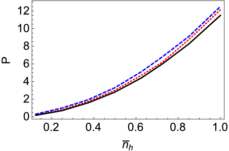
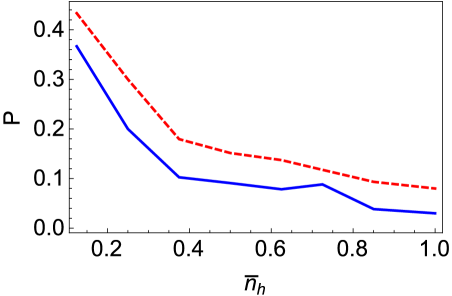
We report the maximum power $P_{\text{max}}$, which is evaluated for the maximum $\langle n_{b}\rangle$ in the steady state, in Fig. 9. After $\bar{n}_{h}\sim 0.325$ the coherent character of the LF mode steady state becomes more significant than its thermal character (cf. Fig. 5), and hence the dissipated power has more useful work content than the incoherent energy. The other two curves in the figure corresponds to the results of the semiclassical and classical models of the system. The semiclassical model, as described in the preceding subsection about the engine cycle, ignores the quantum correlations and factorizes the two operator products $\langle\hat{n}_{a}q\rangle$ and $\langle\hat{n}_{a}p\rangle$ (see their equations of motion in the Appendix.). We will describe the classical model next and explain the hierarchy of the curves in Fig. 9 in terms of the classical and quantum correlations. We note that as $\bar{n}_{h}$ grows, the quantum correlations are less significant. The relative difference between the classical and quantum descriptions diminish with increasing temperature as shown in Fig. 10.

Figure 11: (Colour online) Change in the internal energy $U$ of the classical engine with respect to the effective frequency $\omega_{\text{eff}}$ for $\bar{n}_{\text{h}}=0.125$. We use the frequency of the HF resonator $\omega_{a}$ to make our parameters scaled and dimensionless. All the other parameters are as explained in the text.

IV Classical model

In order to distinguish quantum features in our engine system from its classical counterpart, we shall now treat the model Hamiltonian in Eq. 1 as a classical model. Replacing the operators of the fields of the resonators with the $c$-numbers such that $\hat{a}\rightarrow\alpha_{a}$ and $\hat{b}\rightarrow\alpha_{b}$ we get the classical Langevin equations

$$\dot{\alpha}_{a} = -\left(i\omega_{a}-ig(\alpha_{b}^{*}+\alpha_{b})+\frac{\kappa_{h}}{2}+\frac{\kappa_{a}}{2}\right)\alpha_{a}$$ (21)

$$+ \xi_{h}(t)+\xi_{a}(t),$$

$$\dot{\alpha}_{b} = -\left(i\omega_{b}+\frac{\kappa_{b}}{2}\right)\alpha_{b}+ig|\alpha_{a}|^{2}+\xi_{b}(t),$$ (22)

where $\xi_{i}(t)$ with $i=a,b,h$ represents time dependent delta-correlated stochastic noise with $\langle\xi_{i}(t)\rangle=0$ and $\langle\xi_{i}(t_{1})\xi_{i}(t_{2})\rangle:=D_{i}\delta(t_{1}-t_{2})$ where $D_{i}$ is the strength of the noise. The parameter $D_{i}$ is a function of $\kappa_{i}$ according to the fluctuation-dissipation theorem Kubo (1966) such that $D_{i}=\kappa_{i}\bar{n}_{i}$.

Figure 12: (Colour online) Phase portrait $X_{b}-Y_{b}$ of the classical LM resonator for $\bar{n}_{\text{h}}=0.125$. All the other parameters are as explained in the text.

We define the field quadratures $X_{i},Y_{i}$ such that $\alpha_{a}:=1/\sqrt{2}(X_{a}+iY_{a})$ and $\alpha_{b}:=1/\sqrt{2}(X_{b}+iY_{b})$. By writing the noise parameters as $\xi_{i}=1/\sqrt{2}(\xi_{x}^{i}+i\xi_{y}^{i})$, we can express the equations to be simulated as

$$dX_{a} = \left[\omega_{a}Y_{a}-g\sqrt{2}X_{b}Y_{a}-\kappa^{\prime}_{a}X_{a}\right]dt$$ (23)

$$+ dW^{h}_{x}+dW^{a}_{x},$$

$$dY_{a} = -\left[\omega_{a}X_{a}-g\sqrt{2}X_{a}X_{b}+\kappa^{\prime}_{a}Y_{a}\right]dt$$ (24)

$$+ dW^{h}_{y}+dW^{a}_{y},$$

$$dX_{b} = \left[\omega_{b}Y_{b}-\frac{\kappa_{b}}{2}X_{b}\right]dt+dW^{b}_{x},$$ (25)

$$dY_{b} = -\left[\omega_{b}X_{b}+\frac{\kappa_{b}}{2}Y_{b}-\frac{g}{\sqrt{2}}(X_{a}^{2}+Y_{a}^{2})\right]dt$$ (26)

$$+ dW^{b}_{y}.$$

Here, $dW^{i}=1/\sqrt{2}(dW_{x}^{i}+idW_{y}^{i})$ where $\xi_{k}^{i}dt=:dW_{k}^{i}$, with $k=x,y$, is the Wiener process with width $\sqrt{\kappa_{i}\bar{n}_{i}dt}$ and $\kappa^{\prime}_{a}:=\kappa_{h}/2+\kappa_{a}/2$. For the cooling stage, $\kappa^{\prime}_{a}$ is replaced by $\kappa_{a}/2$ and the $dW^{h}_{x},dW^{h}_{y}$ terms vanish.

The physical parameters used in the classical dynamical simulations are the same as those used in the quantum case. The equations are solved by using Mathematica 10.

V Results of classical simulations

In Fig. 11, we present the change in the internal energy $U_{a}$ of the classical engine with respect to $\omega_{\text{eff}}$ for $\bar{n}_{h}=0.125$. The result follows and fluctuates about the semiclassical cycle in Fig. 6, as expected theoretically. Similarly, the phase portrait of the classical engine in Fig. 12 is the same with its quantum counterpart in Fig. 4. Theoretically, the quantum dynamics of $\langle\hat{n}_{a}\rangle$ and the phase space quadratures are the same for the classical and quantum mechanical descriptions. Factorization of the two operator expectation value $\langle\hat{n}_{a}\hat{q}\rangle$ to define $\omega_{\text{eff}}$ makes the semiclassical $U_{a}-\omega_{\text{eff}}$ cycle identical with the classical one.

Fig. 9 shows the maximum power output of the classical engine with respect to $\bar{n}_{h}$. The power output of the classical engine lies between the quantum and semiclassical models. The difference of quantum model from the classical and the semiclassical models is more significant in the dissipated power output of the LF resonator in contrast to negligible difference between the classical and quantum treatment of the extractable work from the HF resonator. The differences diminish with increasing temperature of the driving noise as shown in Fig. 10. In order to explain such different effects of correlations on different subsystems of the engine, we investigate the classical and quantum correlations more closely in the next section. We note that power enhancement in the coherent work extraction relative to the stochastic one has been discussed in the literature as a signature of the quantum character of certain quantum heat engines, different than our system. Quantum coherence has been suggested as the main source of the power enhancement Uzdin et al. (2015). It has been conjectured that quantum correlations (entanglement or discord) in multiparticle engines could play a similar role to that of coherence in single particle engines. Our two coupled resonator set up can be envisioned as an example to verify this conjecture. As the systems are different, we need to elaborate explicitly if and how the quantum and classical correlations emerge in our system and how they lead to enhanced power output in our case.

VI Quantum nature of the system

The equations of motion for the dynamical variables of interest in our system are given in the Appendix A. In this section, we will discuss the set of equations related to the correlations contributing to the power and work output of our quantum heat engine.

The extractable work depends on the pressure- displacement correlation $\langle\hat{n}_{a},\hat{q}\rangle$, where the correlation function for two operators $\hat{o}_{1}$ and $\hat{o}_{2}$ is defined as $\langle\hat{o}_{1},\hat{o}_{2}\rangle=\langle\hat{o}_{1}\hat{o}_{2}\rangle-\langle\hat{o}_{1}\rangle\langle\hat{o}_{2}\rangle$. According to Eq. (19), the power output of the Otto cycle of the HF resonator depends on the pressure-momentum correlation $\langle\hat{n}_{a},\hat{p}\rangle$. Both the pressure-displacement and pressure-momentum correlations are driven by the number fluctuations of the HF mode which is thermally excited by the hot reservoir. This mechanism is described by the closed system of equations given in Appendix A. We can find the equation of motion for $\langle\hat{n}_{a},\hat{q}\rangle$ as

$$\left(\frac{d^{2}}{dt^{2}}+2C\frac{d^{2}}{dt}+\omega^{2}\right)\langle\hat{n}_{a},\hat{q}\rangle=2g\omega_{b}\langle(\Delta\hat{n}_{a})^{2}\rangle,$$ (27)

where $C=\kappa_{h}+\kappa_{a}+\kappa_{b}/2$ and $\omega=\omega_{b}^{2}+C^{2}$. system of equations for $\langle(\Delta\hat{n}_{a})^{2}\rangle$, $\langle\hat{n}_{a},\hat{q}\rangle$, and $\langle\hat{n}_{a},\hat{p}\rangle$ is parallel to that of $\langle\hat{n}_{a}\rangle$, $\langle\hat{q}\rangle$, and $\langle\hat{p}\rangle$. $\langle(\Delta\hat{n}_{a})^{2}\rangle$ and $\langle\hat{n}_{a}\rangle$ have similar temporal profiles, with the same periodicity but with different amplitudes. Accordingly, $\langle\hat{n}_{a},\hat{q}\rangle$ exhibits a periodically-driven underdamped oscillatory motion, which is analogous to the dynamics of $q$. In contrast to the case of $q$, however, the weak damping condition $C<\omega$ is weakly satisfied and the correlation dynamics are in a regime which is only slightly beyond critical damping (since $C\sim 2\kappa_{a}\gg\omega_{b}$).

Figure 13: (Colour online) Relation between the dynamics of the quantum correlations $\langle\hat{n}_{a},\hat{q}\rangle$ and $\langle\hat{n}_{a},\hat{q}\rangle$. A closed cycle emerges in the steady state as both correlations are slaved by the number fluctuation dynamics of HF resonator. $\langle\hat{n}_{a},\hat{p}\rangle$ varies over a much wider range than the $\langle\hat{n}_{a},\hat{q}\rangle$. All the other parameters are as explained in the text.

The formal solution of the $\langle\hat{n}_{a},\hat{q}\rangle$ can be written as

$$\langle\hat{n}_{a},\hat{q}\rangle=\int_{0}^{t}dt^{\prime}e^{-C(t-t^{\prime})}\sin{(\omega_{b}(t-t^{\prime}))}f(t^{\prime}),$$ (28)

with $f(t)=2g\langle(\Delta\hat{n}_{a})^{2}(t)\rangle$. Another difference from the $q$ dynamics, which has a resonant drive, is that the natural frequency $\omega\sim 2\kappa_{a}$ of the correlation oscillator is far off resonant with the drive frequency $\omega_{b}$. In this case, the fast correlations adiabatically follows the slow fluctuations of the HF resonator. We can employ integration by parts to the formal solution to show that

$$\langle\hat{n}_{a},\hat{q}\rangle\approx\frac{g\omega_{b}}{2\kappa_{a}^{2}}\langle(\Delta\hat{n}_{a})^{2}\rangle(1-e^{-Ct}).$$ (29)

In the long-time limit the steady state at the end of the heating and cooling cycles coincides with the exact steady state for the continuous drive case discussed in the Appendix B. In terms of our parameter values, this value is too small ($\sim 10^{-3}$) to be of significance for the extractable work from the working HF resonator. On the other hand, using the relation

$$\langle\hat{n}_{a},\hat{p}\rangle=\frac{1}{\omega_{b}}\left(\frac{d}{dt}+C\right)\langle\hat{n}_{a},\hat{q}\rangle,$$ (30)

we get

$$\langle\hat{n}_{a},\hat{p}\rangle=\frac{g}{\kappa_{a}}\langle(\Delta\hat{n}_{a})^{2}\rangle,$$ (31)

which turns out to be an order of magnitude greater than $\langle\hat{n}_{a},\hat{q}\rangle$. Their mutual dynamics are plotted in Fig. 13. According to the Eq. (19), instead of contributing to the work output, $\langle\hat{n}_{a},\hat{p}\rangle$ contributes to power output of the Otto cycle of the HF mode.

We note that a similar parameter to $\langle\hat{n}_{a},\hat{p}\rangle$ (normalized by the variances of the $\hat{n}_{a}$ and $\hat{p}$) has been proposed in the context of the quality of quantum nondemolition measurements and called the signal-meter entanglement parameter Holland et al. (1990). To make analogous notation we use $\Sigma:=-\langle\hat{n}_{a},\hat{p}\rangle$. It has also been used in optomechanical systems as an indicator of quantum coherence Mancini et al. (1997). When $\Sigma<0$, signal-meter type quantum correlations make a positive contribution to the rate of increase of the power output from the LF resonator. The time dependence of $\Sigma$ is shown in in Fig. 14. It is oscillatory, adiabatically following the number fluctuations in the HF resonator, and it is always negative. Similar oscillations in $\Sigma$ are found for a typical optomechanical set up where the drive is coherent. It was proposed that the correlated state can be used to generate a mixture of Cat states through conditional measurement Mancini et al. (1997). In our case, coherence and correlations are driven by an incoherent drive.

Figure 14: (Colour online) Dynamics of the correlation function $\Sigma$ with respect to the scaled time $\omega_{\text{a}}t$ for (a) $\bar{n}_{\text{h}}=0.125$ and (b) $\bar{n}_{\text{h}}=1$ calculated by quantum (solid blue curves) and classical (red noisy curves) methods. All the other parameters are as explained in the text.

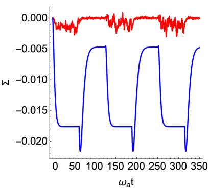
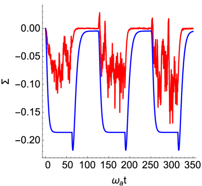
We have also calculated the classical correlation $\Sigma_{\text{class}}=-\langle\hat{n}_{a},\hat{p}\rangle_{\text{class}}$. Here $\langle.\rangle_{\text{class}}$ indicates averaging over classical trajectories. The results are plotted in Fig. 14. This shows that there is a difference between the amplitudes of the quantum and classical correlations. The quantum model predicts a faster growth rate and higher maximum value for the power output from the LF resonator relative to the classical model. Both models predict more powerful and faster engines relative to the semiclassical model.

VII Conclusions

In summary, we proposed and investigated a pair of superconducting transmission line resonators with an optomechanical-like interaction as a quantum heat engine. The high frequency (HF) resonator is periodically coupled to an effective hot bath while both resonators are coupled to continuous effective cold baths. We found the emergence of a limit cycle in the open system dynamics and identified that the HF resonator mode undergoes an effective Otto cycle. The electromagnetic field mode of the HF resonator acts as the working substance while the mode of the LF one acts as the piston that can be used for coherent power extraction. The superconducting resonator engine serves as an electrical analog of a mechanical piston engine. We found that a piston-like motion can be identified in the phase space by using the phase portraits and Wigner function plots. We numerically verified, by calculating the second order coherence function, that the working resonator remains thermal while the “piston” resonator is “charged” to a thermal coherent state, which is a thermodynamically non-passive state that can be used to harvest useful work Gelbwaser-Klimovsky and Kurizki (2015).

Extractable work and efficiency has been calculated from the T-S diagram and from the internal energy diagram. We found that pressure-displacement correlations could in principle contribute to the enhancement of extractable work. However, the effect is negligible. A practical figure of merit for the piston engine performance is the dissipative power from the piston subsystem. When we evaluate it, we found that pressure-momentum correlations (also known as signal-meter type correlations) contribute significantly. These correlations are driven by the variance of the working resonator, which is driven by the thermal fluctuations of the hot reservoir. By this way, in addition to the mean number of excitations in the hot bath, its fluctuations can be harvested through the dissipative power of the piston resonator. This is not a universal conclusion. In other optomechanical quantum piston engines quantum correlations could lead to a power increase only in limited parameter regimes Mari et al. (2015) or could even be harmful to the output power Roulet et al. (2017). We compared the classical, semiclassical, and quantum engine descriptions and concluded that our engine is inevitably a genuine quantum heat engine with enhanced power output due to quantum correlations so that it could be used as a test bed to explore quantum effects in quantum engine cycles.

Here we have only considered classical noise drives, however our framework is applicable to the case of quantum noise drives as well. According to our analytical results, we conclude that the quantum enhancement in the power output can be further increased by using quantum drives instead of classical drives. For example, using a squeezed thermal noise, number fluctuations could be increased to enlarge the pressure-displacement or pressure-momentum correlations to make the quantum enhancement in the work or power output more significant relative to classical engines Roßnagel et al. (2014); Klaers et al. (2017).

Our results could be practically significant for realization of compact, on-chip, scalable, electronic realizations of genuine quantum heat engines with quantum coherence and correlations advantages relative to their classical counterparts. It can also fundamentally be used as a testbed to explore the quantum-to-classical transition of heat engines and to illuminate the role of quantum correlations in the operation of quantum heat engines.

Appendix A Quantum dynamics of the model system

A “gobal” master equation, also called the “dressed state master equation (DSME)”, which is applicable to a system with arbitrarily strong optomechanical coupling has been derived in Ref. Hu et al. (2015) and expressed in the Schroödinger picture as $(\hbar=1,k_{B}=1)$

$$\dot{\hat{\rho}} = -i[\hat{H}_{\text{sys}},\hat{\rho}]$$

$$+ \kappa_{a}(\bar{n}_{a}+1)D[\hat{a}]+\kappa_{a}\bar{n}_{a}D[\hat{a}^{\dagger}]$$

$$+ \kappa_{\text{h}}(t)(\bar{n}_{\text{h}}+1)D[\hat{a}]+\kappa_{h}(t)\bar{n}_{\text{h}}D[\hat{a}^{\dagger}]$$

$$+ \alpha^{2}\kappa_{\text{d}}D[\hat{a}^{\dagger}\hat{a}]$$

$$+ \kappa_{b}(\bar{n}_{b}+1)D[\hat{b}-\alpha\hat{a}^{\dagger}\hat{a}]+\kappa_{b}\bar{n}_{b}D[\hat{b}^{\dagger}-\alpha\hat{a}^{\dagger}\hat{a}],$$

where $\alpha=g/\omega_{b}$ characterizes the “non-local’ effects of the reservoirs and $\kappa_{\text{d}}=4\kappa_{b}T_{b}/\omega_{b}$ is the dephasing rate of the HF resonator mode. This expression is obtained under the assumption that the bath of the LF resonator has an Ohmic spectral density. The interaction of the HF resonator mode with the baths attached to it remain approximately local as $\omega_{a}\gg\omega_{b}$ so that “phonon” side modes do not change the spectral densities of the baths of the HF resonator. This requires the spectral densities to be slowly varying near the resonance frequency $\omega_{a}$. These are consistent with the conditions we employ on the noise drives applied to the resonators.

Equations of motions for the relevant dynamical observables of our system are determined from the master equation and given by

$$\frac{d}{dt} \langle\hat{n}_{a}\rangle=A-B\langle\hat{n}_{a}\rangle,$$ (33)

$$\frac{d}{dt} \langle\hat{p}\rangle=-\omega_{b}\langle\hat{q}\rangle-\frac{\kappa_{b}}{2}\langle\hat{p}\rangle+2g\langle\hat{n}_{a}\rangle,$$ (34)

$$\frac{d}{dt} \langle\hat{q}\rangle=\omega_{b}\langle\hat{p}\rangle-\frac{\kappa_{b}}{2}\langle\hat{q}\rangle+\alpha\kappa_{b}\langle\hat{n}_{a}\rangle,$$ (35)

$$\frac{d}{dt} \langle(\Delta\hat{n}_{a})^{2}\rangle=A+(2A+B)\langle\hat{n}_{a}\rangle-2B\langle(\Delta\hat{n}_{a})^{2}\rangle,$$ (36)

$$\frac{d}{dt} \langle\hat{n}_{a},\hat{p}\rangle=-C\langle\hat{n}_{a},\hat{p}\rangle-\omega_{b}\langle\hat{n}_{a},\hat{q}\rangle+2g\langle(\Delta\hat{n}_{a})^{2}\rangle,$$ (37)

$$\frac{d}{dt} \langle\hat{n}_{a},\hat{q}\rangle=-C\langle\hat{n}_{a},\hat{q}\rangle+\omega_{b}\langle\hat{n}_{a},\hat{p}\rangle+\alpha\kappa_{b}\langle(\Delta\hat{n}_{a})^{2}\rangle,$$ (39)

$$\frac{d}{dt} \langle\hat{n}_{b}\rangle=-\kappa_{b}(\langle\hat{n}_{b}\rangle-\bar{n}_{b})+g(\langle\hat{n}_{a},\hat{p}\rangle+\langle\hat{n}_{a}\rangle\langle\hat{p}\rangle)$$

$$+\alpha\frac{\kappa_{b}}{2}(\langle\hat{n}_{a},\hat{q}\rangle+\langle\hat{n}_{a}\rangle\langle\hat{q}\rangle),$$

where $\hat{q}=\hat{b}+\hat{b}^{\dagger}$, $\hat{p}=i(\hat{b}-\hat{b}^{\dagger})$, $A=\kappa_{a}\bar{n}_{a}+\kappa_{h}\bar{n}_{h}$, $B=\kappa_{a}+\kappa_{h}$, and $C=B+\kappa_{b}/2$. Correlation function between the two dynamical observables with the operators $\hat{o}_{1}$ and $\hat{o}_{2}$ are denoted by $\langle\hat{o}_{1},\hat{o}_{2}\rangle=\langle\hat{o}_{1}\hat{o}_{2}\rangle-\langle\hat{o}_{1}\rangle\langle\hat{o}_{2}\rangle$. The terms with parameter $\alpha$ are due to the non-local effects of the reservoir-system interactions. In the range of our interest, $g\leq\omega_{b}$ we did not find any significant effects due to them, except a negligible increase in $\langle\hat{n}_{a},\hat{q}\rangle$. We use the local master equation and the corresponding equations of motion by taking $\alpha=0$ unless otherwise noted in the manuscript.

We note that the closed dynamics that we have found for the set of thermodynamically relevant observables cannot be found for all dynamical variables of the system. The optomechanical Hamiltonian has a special symmetry in which the number operator of the HF resonator mode is a constant of motion. The steady state of the HF resonator and the associated local observables for the HF mode are independent of the optomechanical coupling coefficient $g$ Bernád and Torres (2015). The first three equations of motion form a closed set of dynamics for the $q-p$ phase space trajectories, driven by $\langle\hat{n}_{a}\rangle$. The second set of three equations form another, inpendent, closed set of dynamics for the “pressure-displacement”, $\langle\hat{n}_{a},\hat{q}\rangle$, and “pressure-momentum”, $\langle\hat{n}_{a},\hat{p}\rangle$ correlations, driven by the quantum fluctuations $\langle(\Delta\hat{n}_{a})^{2}\rangle$. The baths of the HF resonator mode prepare the pressure ($\sim\langle\hat{n}_{a}\rangle$ and quantum noise drives for these independent dynamics. Both dynamics contribute to the evolution of the excitations in the LF mode given in the last equation.

Appendix B Steady state of the quantum dynamics under continuous heating

While the dynamics of the LF mode is different under pulsed thermal drive, the HF resonator reaches approximately its steady state identical with a continuous drive case, for the pulse duration is longer than its thermalization transition time. In order to highlight the effect of pulsed drive relative to continuous drive on the LF mode dynamics, and to give steady state values of the HF dynamics as well, we provide the solutions of the quantum dynamical equations in the Appendix A in the long time limit below and note some common characteristic behaviors.

$$\langle\hat{n}_{a}\rangle_{\text{SS}} = \frac{A}{B}=\frac{\kappa_{a}\bar{n}_{a}+\kappa_{h}\bar{n}_{h}}{\kappa_{a}+\kappa_{h}},$$ (40)

$$\langle\hat{q}\rangle_{\text{SS}} = \frac{8g\omega_{b}+4\alpha\kappa_{b}^{2}}{4\omega_{b}^{2}+\kappa_{b}^{2}}\langle\hat{n}_{a}\rangle_{\text{SS}},$$ (41)

$$\langle\hat{p}\rangle_{\text{SS}} = \frac{4g\kappa_{b}-4\alpha\kappa_{b}\omega_{b}}{4\omega_{b}^{2}+\kappa_{b}^{2}}\langle\hat{n}_{a}\rangle_{\text{SS}}=0,$$ (42)

$$\langle(\Delta\hat{n}_{a})^{2}\rangle_{\text{SS}} = \frac{A(A+B)}{B^{2}},$$ (43)

$$\langle\hat{n}_{a},\hat{p}\rangle_{\text{SS}} = \frac{2gC-\alpha\kappa_{b}\omega_{b}}{\omega_{b}^{2}+C^{2}}\langle(\Delta\hat{n}_{a})^{2}\rangle_{\text{SS}},$$ (44)

$$= \frac{2gB}{\omega_{b}^{2}+C^{2}}\langle(\Delta\hat{n}_{a})^{2}\rangle_{\text{SS}},$$ (45)

$$\langle\hat{n}_{a},\hat{q}\rangle_{\text{SS}} = \frac{2g\omega_{b}+\alpha\kappa_{b}C}{\omega_{b}^{2}+C^{2}}\langle(\Delta\hat{n}_{a})^{2}\rangle_{\text{SS}},$$ (46)

$$\langle\hat{n}_{b}\rangle_{\text{SS}} = \bar{n}_{b}+\frac{g}{\kappa_{b}}(\langle\hat{n}_{a},\hat{p}\rangle_{\text{SS}}+\langle\hat{n}_{a}\rangle_{\text{SS}}\langle\hat{p}\rangle_{\text{SS}})$$ (47)

$$+ \frac{\alpha}{2}(\langle\hat{n}_{a},\hat{q}\rangle+\langle\hat{n}_{a}\rangle\langle\hat{q}\rangle)$$

According to our parameters we have $\kappa_{a}=\kappa_{h}$ so that $\langle\hat{n}_{a}\rangle_{\text{SS}}=(\bar{n}_{c}+\bar{n}_{h})/2$. In addition, the variance becomes $\langle(\Delta\hat{n}_{a})^{2}\rangle_{\text{SS}}\sim(\bar{n}_{a}+\bar{n}_{h})(\bar{n}_{a}+\bar{n}_{h}+2)/4$. Exact solution of the pulsed drive case yields these value to a very good approximation, conforming that the pulse duration is sufficiently long to thermalize the HF resonator. The steady state values of the LF resonator gives smaller $\langle\hat{n}_{b}\rangle_{\text{SS}}$ in the case of continuous drive. A common behavior under both the continuous or pulsed drive is the quadratic increase of $\langle\hat{n}_{b}\rangle_{\text{SS}}$ with $\bar{n}_{h}$. Both the correlation term $\langle\hat{n}_{a},\hat{p}\rangle_{\text{SS}}$ and the factorized semi-classical term $\langle\hat{n}_{a}\rangle_{\text{SS}}\langle\hat{p}\rangle_{\text{SS}}$ increase quadratically with $\bar{n}_{h}$. This behavior is translated to the power output of the engine, which is proportional to $P\propto\langle\hat{n}_{b}\rangle_{\text{SS}}-\bar{n}_{b}$.

Appendix C Steady state of the electric displacement under periodic heating

The equation motion of $q$

$$\ddot{q}+\kappa_{b}\dot{q}+\omega^{2}q=2\omega_{b}g\langle n_{a}(t)\rangle,$$ (48)

with $\omega^{2}=\omega_{b}^{2}+\kappa_{b}^{2}/4$, can be solved in steady state by approximating the $\langle\hat{n}_{a}\rangle$ by a square wave with period $T=2\pi/\omega_{b}$. Transforming $q\rightarrow q=Q+q_{0}$ we write

$$\ddot{Q}+\kappa_{b}\dot{Q}+\omega^{2}Q=2\omega_{b}g\langle F_{a}(t)\rangle,$$ (49)

where $F(t)$ is made to be periodically alternating between $\pm(\bar{n}_{h}-\bar{n}_{c})/4$ by taking

$$q_{0}=\frac{2\omega_{b}g}{\omega^{2}}\left(\frac{\bar{n}_{h}+3\bar{n}_{c}}{4}\right).$$ (50)

First harmonic at frequency $\omega_{b}$ is then given by

$$Q=\frac{4}{\pi}\frac{2\omega_{b}g}{\sqrt{\kappa_{b}^{2}\left(\omega_{b}^{2}+\frac{\kappa_{b}^{2}}{16}\right)}}\left(\frac{\bar{n}_{h}-\bar{n}_{c}}{4}\right)\sin{(\omega_{b}t+\alpha)},$$ (51)

where

$$\alpha=\arctan{\left(\frac{\kappa_{b}\omega_{b}}{\omega_{b}^{2}-\omega^{2}}\right)}.$$ (52)

References

- (1) T. D. Kieu, The second law, maxwell’s demon, and work derivable from quantum heat engines, Phys. Rev. Lett. 93, 140403.
- Quan et al. (2007) H. T. Quan, Y.-x. Liu, C. P. Sun, and F. Nori, Quantum thermodynamic cycles and quantum heat engines, Phys. Rev. E 76, 031105 (2007).
- Quan et al. (2005) H. T. Quan, P. Zhang, and C. P. Sun, Quantum heat engine with multilevel quantum systems, Phys. Rev. E 72, 056110 (2005).
- Abah et al. (2012) O. Abah, J. Roßnagel, G. Jacob, S. Deffner, F. Schmidt-Kaler, K. Singer, and E. Lutz, Single-Ion Heat Engine at Maximum Power, Phys. Rev. Lett. 109, 203006 (2012).
- Bergenfeldt et al. (2014) C. Bergenfeldt, P. Samuelsson, B. Sothmann, C. Flindt, and M. Büttiker, Hybrid microwave-cavity heat engine, Phys. Rev. Lett. 112, 076803 (2014).
- Henrich et al. (2007) M. J. Henrich, G. Mahler, and M. Michel, Driven spin systems as quantum thermodynamic machines: Fundamental limits, Phys. Rev. E 75, 051118 (2007).
- Uzdin and Kosloff (2014) R. Uzdin and R. Kosloff, The multilevel four-stroke swap engine and its environment, New J. Phys. 16, 095003 (2014).
- Scully et al. (2003) M. O. Scully, M. S. Zubairy, G. S. Agarwal, and H. Walther, Extracting work from a single heat bath via vanishing quantum coherence, Science 299, 862 (2003).
- Scully et al. (2011) M. O. Scully, K. R. Chapin, K. E. Dorfman, M. B. Kim, and A. Svidzinsky, Quantum heat engine power can be increased by noise-induced coherence, Proc. Natl. Acad. Sci. 108, 15097 (2011).
- Scully (2010) M. O. Scully, Quantum photocell: Using quantum coherence to reduce radiative recombination and increase efficiency, Phys. Rev. Lett. 104, 207701 (2010).
- Brunner et al. (2012) N. Brunner, N. Linden, S. Popescu, and P. Skrzypczyk, Virtual qubits, virtual temperatures, and the foundations of thermodynamics, Phys. Rev. E 85, 051117 (2012).
- Manzano et al. (2016) G. Manzano, F. Galve, R. Zambrini, and J. M. R. Parrondo, Entropy production and thermodynamic power of the squeezed thermal reservoir, Phys. Rev. E 93, 052120 (2016).
- Song et al. (2016) Q. Song, S. Singh, K. Zhang, W. Zhang, and P. Meystre, One atom and one photon - the simplest polaritonic heat engine, arXiv:1607.00119 [quant-ph] (2016), arXiv: 1607.00119.
- Altintas et al. (2015) F. Altintas, A. Ü. C. Hardal, and Ö. E. Müstecaplıoğlu, Rabi model as a quantum coherent heat engine: From quantum biology to superconducting circuits, Phys. Rev. A 91, 023816 (2015).
- Ivanchenko (2015) E. A. Ivanchenko, Quantum Otto cycle efficiency on coupled qudits, Phys. Rev. E 92, 032124 (2015).
- Altintas et al. (2014) F. Altintas, A. Ü. C. Hardal, and Ö. E. Müstecaplıog̃lu, Quantum correlated heat engine with spin squeezing, Phys. Rev. E 90, 032102 (2014).
- Dağ et al. (2016) C. B. Dağ, W. Niedenzu, Ö. E. Müstecaplıoğlu, and G. Kurizki, Multiatom Quantum Coherences in Micromasers as Fuel for Thermal and Nonthermal Machines, Entropy 18, 244 (2016).
- Türkpençe and Müstecaplıoğlu (2016) D. Türkpençe and Ö. E. Müstecaplıoğlu, Quantum fuel with multilevel atomic coherence for ultrahigh specific work in a photonic carnot engine, Phys. Rev. E 93, 012145 (2016).
- Hardal and Müstecaplıoğlu (2015) A. Ü. C. Hardal and Ö. E. Müstecaplıoğlu, Superradiant quantum heat engine, Sci. Rep. 5, 12953 (2015).
- Campisi and Fazio (2016) M. Campisi and R. Fazio, The power of a critical heat engine, Nat. Comm. 7, 11895 (2016).
- Kosloff and Levy (2014) R. Kosloff and A. Levy, Quantum Heat Engines and Refrigerators: Continuous Devices, Annu. Rev. Phys. Chem. 65, 365 (2014).
- Tonner and Mahler (2005) F. Tonner and G. Mahler, Autonomous quantum thermodynamic machines, Phys. Rev. E 72, 066118 (2005).
- Anders and Giovannetti (2013) J. Anders and V. Giovannetti, Thermodynamics of discrete quantum processes, New J. Phys. 15, 033022 (2013).
- Zhang et al. (2014a) K. Zhang, F. Bariani, and P. Meystre, Quantum Optomechanical Heat Engine, Phys. Rev. Lett. 112, 150602 (2014a).
- Zhang et al. (2014b) K. Zhang, F. Bariani, and P. Meystre, Theory of an optomechanical quantum heat engine, Phys. Rev. A 90, 023819 (2014b).
- Zhang and Zhang (2017) K. Zhang and W. Zhang, Quantum optomechanical straight-twin engine, Phys. Rev. A 95, 053870 (2017).
- Mari et al. (2015) A. Mari, A. Farace, and V. Giovannetti, Quantum optomechanical piston engines powered by heat, J. Phys. B At. Mol. Opt. Phys. 48, 175501 (2015).
- Gelbwaser-Klimovsky and Kurizki (2015) D. Gelbwaser-Klimovsky and G. Kurizki, Work extraction from heat-powered quantized optomechanical setups, Sci. Rep. 5, 7809 (2015).
- Roßnagel et al. (2014) J. Roßnagel, O. Abah, F. Schmidt-Kaler, K. Singer, and E. Lutz, Nanoscale Heat Engine Beyond the Carnot Limit, Phys. Rev. Lett. 112, 030602 (2014).
- Allahverdyan and Nieuwenhuizen (2000) A. E. Allahverdyan and T. M. Nieuwenhuizen, Extraction of Work from a Single Thermal Bath in the Quantum Regime, Phys. Rev. Lett. 85, 1799 (2000).
- Korzekwa et al. (2016) K. Korzekwa, M. Lostaglio, J. Oppenheim, and D. Jennings, The extraction of work from quantum coherence, New J. Phys. 18, 023045 (2016).
- Perarnau-Llobet et al. (2015) M. Perarnau-Llobet, K. V. Hovhannisyan, M. Huber, P. Skrzypczyk, N. Brunner, and A. Acín, Extractable Work from Correlations, Phys. Rev. X 5, 041011 (2015).
- Plastina et al. (2014) F. Plastina, A. Alecce, T. Apollaro, G. Falcone, G. Francica, F. Galve, N. Lo Gullo, and R. Zambrini, Irreversible Work and Inner Friction in Quantum Thermodynamic Processes, Phys. Rev. Lett. 113, 260601 (2014).
- Campo et al. (2014) A. d. Campo, J. Goold, and M. Paternostro, More bang for your buck: Super-adiabatic quantum engines, Sci. Rep. 4, 6208 (2014).
- Roulet et al. (2017) A. Roulet, S. Nimmrichter, J. M. Arrazola, S. Seah, and V. Scarani, Autonomous rotor heat engine, Phys. Rev. E 95, 062131 (2017).
- Hofer et al. (2016a) P. P. Hofer, J.-R. Souquet, and A. A. Clerk, Quantum heat engine based on photon-assisted cooper pair tunneling, Physical Review B 93, 041418 (2016a).
- Hofer et al. (2017a) P. P. Hofer, J. B. Brask, M. Perarnau-Llobet, and N. Brunner, Quantum thermal machine as a thermometer, arXiv preprint arXiv:1703.03719 (2017a).
- Hofer et al. (2016b) P. P. Hofer, M. Perarnau-Llobet, J. B. Brask, R. Silva, M. Huber, and N. Brunner, Autonomous quantum refrigerator in a circuit qed architecture based on a josephson junction, Physical Review B 94, 235420 (2016b).
- Karimi and Pekola (2016) B. Karimi and J. Pekola, Otto refrigerator based on a superconducting qubit: Classical and quantum performance, Physical Review B 94, 184503 (2016).
- Roßnagel et al. (2016) J. Roßnagel, S. T. Dawkins, K. N. Tolazzi, O. Abah, E. Lutz, F. Schmidt-Kaler, and K. Singer, A single-atom heat engine, Science 352, 325 (2016).
- Uzdin et al. (2015) R. Uzdin, A. Levy, and R. Kosloff, Equivalence of Quantum Heat Machines, and Quantum-Thermodynamic Signatures, Phys. Rev. X 5, 031044 (2015).
- Mukherjee et al. (2016) V. Mukherjee, W. Niedenzu, A. G. Kofman, and G. Kurizki, Speed and Efficiency Limits of Multilevel Incoherent Heat Engines, arXiv:1607.08452 [cond-mat, physics:quant-ph] (2016), arXiv: 1607.08452.
- Quan et al. (2006) H. T. Quan, P. Zhang, and C. P. Sun, Quantum-classical transition of photon-Carnot engine induced by quantum decoherence, Phys. Rev. E 73, 036122 (2006).
- Johansson et al. (2014) J. R. Johansson, G. Johansson, and F. Nori, Optomechanical-like coupling between superconducting resonators, Phys. Rev. A 90, 053833 (2014).
- Holland et al. (1990) M. Holland, M. Collett, D. Walls, and M. Levenson, Nonideal quantum nondemolition measurements, Phys. Rev. A 42, 2995 (1990).
- Mancini et al. (1997) S. Mancini, V. Man’ko, and P. Tombesi, Ponderomotive control of quantum macroscopic coherence, Phys. Rev. A 55, 3042 (1997).
- Fink et al. (2010) J. M. Fink, L. Steffen, P. Studer, L. S. Bishop, M. Baur, R. Bianchetti, D. Bozyigit, C. Lang, S. Filipp, P. J. Leek, and A. Wallraff, Quantum-To-Classical Transition in Cavity Quantum Electrodynamics, Phys. Rev. Lett. 105, 163601 (2010).
- Levy and Kosloff (2014) A. Levy and R. Kosloff, The local approach to quantum transport may violate the second law of thermodynamics, Europhys. Lett. 107, 20004 (2014).
- Hofer et al. (2017b) P. P. Hofer, M. Perarnau-Llobet, L. D. M. Miranda, G. Haack, R. Silva, J. B. Brask, and N. Brunner, Markovian master equations for quantum thermal machines: local vs global approach, arXiv preprint arXiv:1707.09211 (2017b).
- González et al. (2017) J. O. González, L. A. Correa, G. Nocerino, J. P. Palao, D. Alonso, and G. Adesso, Testing the validity of the local and global gkls master equations on an exactly solvable model, arXiv preprint arXiv:1707.09228 (2017).
- Hu et al. (2015) D. Hu, S.-Y. Huang, J.-Q. Liao, L. Tian, and H.-S. Goan, Quantum coherence in ultrastrong optomechanics, Phys. Rev. A 91, 013812 (2015).
- (52) J. Teufel, T. Donner, D. Li, J. Harlow, M. Allman, K. Cicak, A. Sirois, J. D. Whittaker, K. Lehnert, and R. W. Simmonds, Sideband cooling of micromechanical motion to the quantum ground state, Nature 475, 359.
- Johansson et al. (2013) J. Johansson, P. Nation, and F. Nori, Qutip 2: A python framework for the dynamics of open quantum systems, Comput. Phys. Commun. 184, 1234 (2013).
- Feldmann and Kosloff (2004) T. Feldmann and R. Kosloff, Characteristics of the limit cycle of a reciprocating quantum heat engine, Phys. Rev. E 70, 046110 (2004).
- da Silva et al. (2010) M. P. da Silva, D. Bozyigit, A. Wallraff, and A. Blais, Schemes for the observation of photon correlation functions in circuit QED with linear detectors, Phys. Rev. A 82, 043804 (2010).
- Klaers et al. (2017) J. Klaers, S. Faelt, A. Imamoglu, and E. Togan, Squeezed thermal reservoirs as a resource for a nano-mechanical engine beyond the Carnot limit, arXiv:1703.10024 [cond-mat] (2017).
- Kubo (1966) R. Kubo, The fluctuation-dissipation theorem, Rep. Prog. Phys. 29, 255 (1966).
- Bernád and Torres (2015) J. Z. Bernád and J. M. Torres, Partly invariant steady state of two interacting open quantum systems, Phys. Rev. A 92, 062114 (2015).