2 Instituto de Astrofísica La Plata, CONICET-UNLP, Paseo del Bosque s/n, (1900) La Plata, Argentina
11email: lcalcaferro,acorsico,althaus@fcaglp.unlp.edu.ar
Pulsating low-mass white dwarfs in the frame of new evolutionary sequences
Abstract
Context. Many pulsating low-mass white-dwarf stars have been detected in the last years in the field of our Galaxy. Given that some of them exhibit multiperiodic variation of brightness, it is possible to probe their interiors through asteroseismology.
Aims. We aim to present a detailed asteroseismological study of all the known low-mass variable white dwarf stars based on a complete set of fully evolutionary models representative of low-mass He-core white dwarf stars.
Methods. We employed adiabatic radial and nonradial pulsation periods for low-mass white dwarf models with stellar masses ranging from to , that were derived by simulating the nonconservative evolution of a binary system consisting of an initially ZAMS star and a neutron star companion. We estimated the mean period spacing for the stars under study (in the cases where it was possible) and then we used the comparison between the observed period spacing with the average of the computed period spacings for our grid of models to constrain the stellar mass. We also employed the individual observed periods of every known pulsating low-mass white dwarf star, to search for a representative seismological model.
Results. We found that even though the stars under analysis exhibit few periods and the period fits show multiplicity of solutions, it is possible to find seismological models whose mass and effective temperature are in agreement with the values given by spectroscopy, for most of the cases. Unfortunately, we were not able to constrain the stellar masses by employing the observed period spacing because, in general, the periods exhibited by these stars are very few. In the two cases where we could extract the period spacing from the set of observed periods, this method led to values of the stellar masses substantially larger than expected for this type of stars.
Conclusions. The results presented in this work show in the one hand, the need for further photometric searches, and on the other hand, some improvements of the theoretical models, in order to place the asteroseismological results on a firmer ground.
Key Words.:
stars: evolution — stars: interiors — stars: oscillations — stars: variables: other (ELM WD)— white dwarfs1 Introduction
White dwarf (WD) stars are the last stage in the life of the majority of stars (Winget & Kepler 2008; Fontaine & Brassard 2008; Althaus et al. 2010). Most WDs have envelopes rich in H, and they define the spectral class DA WD whose distribution peaks at . It also shows a peak at low mass: . These stars are thought to be the result of strong mass-loss episodes in interactive binary systems, before the He flash during the red giant branch phase of low-mass stars (Althaus et al. (2013); Istrate et al. (2016b), for recent studies). At variance with average WDs with C and O cores, they are expected to contain He cores, since He burning is avoided. Specifically, this interactive binary evolutionary scenario is thought to be the most plausible origin for the so-called extremely low-mass (ELM) WDs, which have masses below .
In the last years, numerous low-mass WDs, including ELM WDs, have been discovered via the ELM survey and the SPY and WASP surveys (see Koester et al. 2009; Brown et al. 2010, 2012; Maxted et al. 2011; Kilic et al. 2011, 2012; Brown et al. 2013; Gianninas et al. 2014a; Kilic et al. 2015; Gianninas et al. 2015). The detection of pulsation (gravity) modes in some of them (Hermes et al. 2012, 2013b, 2013a; Kilic et al. 2015; Bell et al. 2015, 2017) has given rise to a new class of variable white dwarfs, the ELMVs. These pulsating low-mass WDs provide us an exceptional chance for probing the interiors of these stars and eventually to test their formation scenarios by employing the tools of asteroseismology. Since modes in ELMVs are restricted mainly to the core regions (Steinfadt et al. 2010; Córsico et al. 2012b; Córsico & Althaus 2014a), we would be able to constrain their core chemical structure. Furthermore, as shown by stability computations (Córsico et al. 2012b; Van Grootel et al. 2013; Córsico & Althaus 2016), a combination of the mechanism (Unno et al. 1989) and the “convective driving” mechanism (Brickhill 1991), both acting at the H-ionization region, excite long-period modes in agreement with observations. Moreover, some unstable short-period modes could be driven by the mechanism due to stable H burning (Córsico & Althaus 2014b).
In addition to ELM stars, there are several objects considered as their precursors, the so-called pre-ELMs. These stars exhibit metals in their atmospheres (e.g. Gianninas et al. 2014b; Hermes et al. 2014; Istrate et al. 2016b). Interestingly enough, pulsations in a number of objects have been detected in the last years (Maxted et al. 2013, 2014; Zhang et al. 2016; Gianninas et al. 2016; Corti et al. 2016). Evolutionary models that consider only element diffusion cannot explain these properties (e.g. Córsico et al. 2016; Istrate et al. 2016a) and might be an indication that the missing physics could impact also the evolution of the objects on the cooling track (e.g., the thickness of the H envelope). Moreover, there are indications that a pre-ELMV WD will be later observed as an ELMV (Fontaine et al. 2017).
The definition of an ELM WD is still under debate. In the context of the ELM survey, an ELM WD is defined as an object with surface gravity of and effective temperature in the range of (e.g. Brown et al. 2010; Kilic et al. 2011; Brown et al. 2016). In addition, an ELM WD should be part of a tight binary system, and therefore show short-period or high-amplitude velocity variability (e.g. Brown et al. 2017). Córsico & Althaus (2014a) suggests to define an ELM WD as a WD that does not undergo H shell flashes as the pulsational properties are quite different as compared with the systems that experience flashes. However, this mass limit depends on the metallicity of the progenitor stars (Istrate et al. 2016b).
WD asteroseismology has already proven to be a very useful technique for peering into the interior of several pulsating WDs, and it has been applied by employing two different methodologies: one considering stellar models with parametrized chemical composition profiles, and another involving fully evolutionary models characterized by a consistent chemical structure. The former has the advantage of allowing a full exploration of the parameter space (the total mass, the mass of the H envelope, the chemical composition of the core, among others) to find an optimal asteroseismological model. Examples of this approach are the pioneer works by Bradley (1998, 2001). More recent works using this avenue are from Pech et al. (2006); Pech & Vauclair (2006); Bischoff-Kim et al. (2008); Castanheira & Kepler (2008, 2009); Paparó et al. (2013); Bognár et al. (2016) and the recent developments of the core parameterization by Giammichele et al. (2016, 2017a, 2017b). The second approach, developed at La Plata Observatory, is different but complementary as it employs fully evolutionary models which are the result of the complete evolution of the progenitor stars, from the Zero Age Main Sequence (ZAMS) until the WD phase. Examples of the application of this method to GW Virginis stars (pulsating PG1159 stars) are the works by Córsico et al. (2007a, b, 2008, 2009); Kepler et al. (2014) and Calcaferro et al. (2016). Also, it has been applied in DBV WDs (He-rich atmosphere) by Córsico et al. (2012a); Bognár et al. (2014). Regarding ZZ Ceti stars, this approach has been successfully employed by Kepler et al. (2012); Romero et al. (2012, 2013). In particular, this method has the value added that the chemical structure of the background models is consistent with the pre-WD evolution.
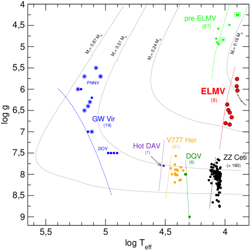
Here, we apply our asteroseismological approach for the first time to the complete set of the known ELMVs, whose spectroscopic parameters we describe in Table 1, and whose list of periods exhibited can be found in Tables 2 to 10, along with the corresponding frequencies and amplitudes. SDSS J184037.78+642312.3 (hereafter J1840) is the first ELMV discovered (Hermes et al. 2012, 2013a). SDSS J111215.82+111745.0 (hereafter J1112) was reported by Hermes et al. (2013b). This case is particularly interesting because this star shows seven periods, and two of them are very short, probably associated with or radial modes. SDSS J151826.68+065813.2 (hereafter J1518) is the hottest ELMV hitherto, according to Hermes et al. (2013b). This star shows seven independent periods, making possible a more detailed asteroseismological analysis. SDSS J161431.28+191219.4 (hereafter J1614) is an ELMV, according to Hermes et al. (2013a). SDSS J222859.93+362359.6 (hereafter J2228) is currently the coolest EMLV, according to Hermes et al. (2013a). This star exhibits only three independent periods in the range s, so these periods seem to be approximately in the asymptotic regime (see Córsico & Althaus 2014a). In particular, the period s is the longest period ever measured in a pulsating WD star. PSR J1738+0333, is a millisecond pulsar that has an ELMV companion (which we shall call, for short, J1738), according to Kilic et al. (2015). This case is particularly interesting because it is the only binary system with a millisecond pulsar and a pulsating WD. SDSS J161831.69+385415.15 (hereafter J1618) is an ELMV, according to Bell et al. (2015). Finally, SDSS J1735+2134 (hereafter J1735) and SDSS J2139+2227 (hereafter J2139) are two recently detected ELMVs, according to Bell et al. (2017). In particular, the former has very long periods, which seem to be in the asymptotic regime of nonradial modes (see Córsico & Althaus 2014a). It is worth mentioning how the spectroscopic masses of the ELM WDs are determined. Brown et al. (2017) showed that for the same metallicity of the progenitor stars there is a 15% difference in the mass of ELM WDs for the same and parameters, using either the Althaus et al. (2013) evolutionary tracks or the Istrate et al. (2016b) evolutionary tracks. We can adopt this difference as the true uncertainty in the spectroscopic determination of the masses of ELM WDs. In Fig. 1 we show the location of the different families of pulsating WDs, including all the known ELMV stars (red circles). The total number of ELMVs rises to nine, because there is a high probability that the star discovered by Bell et al. (2017), SDSS J1355+1956, is a Scuti pulsator, as claimed by these authors. In this sense, it is important to stress here that some of the stars under analysis in this work may not be pulsating ELM WDs. The analysis done by Brown et al. (2017) suggests that there are actually only four pulsating ELM WDs: J1840, J1112, J1518 and J1738. In addition, as discussed by Bell et al. (2015, 2017), the stars J1618, J1735 and J2139 may not be ELM WD stars. A measurement of the rate of period change for these stars could help to shed light on this issue (Calcaferro et al. 2017). Despite of this, given the exploratory nature of this work, we will consider that these stars are genuine ELMVs and they will be included in our analysis.
| Star | Period range | ||||||
|---|---|---|---|---|---|---|---|
| [K] | [cgs] | [] | [K] | [cgs] | [] | [s] | |
| J1840 | 0.183a,b | 0.177c | [1164-4445] | ||||
| J1112 | 0.179d | 0.169c | [108-2856] | ||||
| J1518 | 0.220d | 0.197c | [1335-3848] | ||||
| J1614 | 0.192b | 0.172c | [1184-1263] | ||||
| J2228 | 0.152b | 0.142c | [3255-6235] | ||||
| J1738 | 0.181e | 0.172c | [1788-3057] | ||||
| J1618 | 0.220f | 0.179c | [2543-6126] | ||||
| J1735 | — | — | — | 0.142g | [3363-4961] | ||
| J2139 | — | — | — | 0.149g | [2119-3303] |
In this paper we report a further step in the study of low-mass WD stars by performing an asteroseismological analysis of all the known ELMVs. This is the fifth work of a series dedicated to these stars. The first one (Córsico & Althaus 2014a) was focused on the adiabatic properties of these stars; the second one (Córsico & Althaus 2016) was dedicated to the nonadiabatic pulsation stability features of these stars. The third work (Córsico et al. 2016) was aimed at studying the pulsation properties of the pre-ELMV WDs. The fourth paper (Calcaferro et al. 2017) was focused on studying the theoretical temporal rates of period change of ELMV and pre-ELMV stars. In this work, we follow the approach that employs fully evolutionary models resulting from the complete evolution of the progenitor stars. The employment of fully evolutionary models is a crucial requirement because some models (particularly those with the lowest mass) are characterized by strong H-nuclear burning that depends sensitively on the thickness of the H envelope, a quantity that results from the previous evolution. We employ the adiabatic radial () and non-radial () and mode pulsation periods computed in Córsico & Althaus (2014a) on low-mass He-core WD evolutionary models with stellar masses ranging from to , extracted from the computations of Althaus et al. (2013), that take into account the binary evolution of the progenitor stars.
The paper is organized as follows. A brief summary of the stellar models and the pulsational code employed is provided in Sect. 2. In Sect. 3 we describe the asteroseismological analyses carried out. Next, in Sect. 3.1, we try to determine (when possible) the observed period spacing for the target stars, and then in Sect. 3.2 we constrain the stellar mass by comparing the observed period spacing with the average of the computed period spacings. In Sect. 3.3, we search for the best-fit asteroseismological model by comparing the individual periods from each ELMV star with theoretical periods from our grid of models. Finally, in Sect. 4 we summarize the main findings of this work.
| [s] | Freq.[Hz] | Ampl. [mmag] |
|---|---|---|
| [s] | Freq.[Hz] | Ampl. [mmag] |
|---|---|---|
| [s] | Freq.[Hz] | Ampl. [mmag] |
|---|---|---|
| [s] | Freq.[Hz] | Ampl. [mmag] |
|---|---|---|
| [s] | Freq.[Hz] | Ampl. [mmag] |
|---|---|---|
| [s] | Freq.[Hz] | Ampl. [mmag] |
|---|---|---|
| [s] | Freq.[Hz] | Ampl. [mmag] |
|---|---|---|
| [s] | Freq.[Hz] | Ampl. [mmag] |
|---|---|---|
| [s] | Freq.[Hz] | Ampl. [mmag] |
|---|---|---|
2 Evolutionary models and pulsational code
In this work, we have employed the fully evolutionary models of low-mass He-core WDs generated with the LPCODE stellar evolution code. This code computes in detail the complete evolutionary stages which lead to the WD formation, allowing the study of the WD evolution consistently with the predictions of the evolutionary history of progenitors. Details of LPCODE can be found in Althaus et al. (2005, 2009, 2013, 2015) and references therein. Here, we briefly mention the ingredients employed which are relevant for our analysis of low-mass, He-core WD (see Althaus et al. 2013, for details). The standard Mixing Length Theory (MLT) for convection in the ML2 prescription is used (see Tassoul et al. 1990, for its definition), however adiabatic periods do not sensitively depend on the specific version of the MLT theory of convection employed (Bradley 1998). We assumed the metallicity of the progenitor stars to be . We considered the radiative opacities for arbitrary metallicity in the range of 0 to 0.1 from the OPAL project (Iglesias & Rogers 1996). Conductive opacities are those of Cassisi et al. (2007). For the main sequence evolution, we considered the equation of state from OPAL for H- and He-rich compositions. Also, we have taken from Itoh et al. (1996) the neutrino emission rates for pair, photo, and bremsstrahlung processes, and for plasma processes we included the treatment of Haft et al. (1994). For the WD regime we have employed an updated version of the Magni & Mazzitelli (1979) equation of state. The nuclear network takes into account 16 elements and 34 thermonuclear reaction rates for pp-chains, CNO bi-cycle, He burning, and C ignition. We also considered time-dependent diffusion due to gravitational settling and chemical and thermal diffusion of nuclear species following the multicomponent gas treatment of Burgers (1969). We have computed abundance changes according to element diffusion, nuclear reactions, and convective mixing, a treatment that represents a very significant aspect in evaluating the importance of residual nuclear burning during the cooling stage of low-mass WDs.
The pulsation analysis was carried out for radial () and non-radial () and modes, on the basis of the set of adiabatic and non adiabatic pulsation periods presented in Córsico & Althaus (2014a, 2016), computed employing the adiabatic and non adiabatic versions of the LP-PUL pulsation code (Córsico & Althaus 2006; Córsico et al. 2006). The adiabatic version of the LP-PUL pulsation code is coupled to the LPCODE evolutionary code, and is based on a general Newton-Raphson technique that solves the fourth-order (second-order) set of real equations and boundary conditions governing linear, adiabatic, nonradial (radial) stellar pulsations following the dimensionless formulation of Dziembowski (1971) (see, also, Unno et al. 1989). On the other side, the non-radial (radial) non adiabatic version of the LP-PUL pulsation code solves the sixth-order (fourth-order) complex system of linearized equations and boundary conditions as given by Unno et al. (1989) (Saio et al. 1983). Our nonadiabatic computations rely on the frozen-convection approximation, in which the perturbation of the convective flux is neglected. To compute the Brunt-Väisälä frequency () we follow the so-called “Ledoux Modified” treatment (Tassoul et al. 1990; Brassard et al. 1991).
Regarding the evolutionary sequences, realistic configurations for low-mass He-core WD stars were derived by Althaus et al. (2013) by mimicking the binary evolution of progenitor stars. Binary evolution was assumed to be fully nonconservative, and the losses of angular momentum due to mass loss, gravitational wave radiation, and magnetic braking were considered. All of the He-core WD initial models were derived from evolutionary calculations for binary systems consisting of an evolving Main Sequence low-mass component (donor star) of initially and a neutron star companion as the other component. A total of 14 initial He-core WD models with stellar masses of , , , , , , , , , , , , and were computed for initial orbital periods at the beginning of the Roche lobe phase in the range of to d. The evolution of these models was computed down to the range of luminosities of cool WDs, including the stages of multiple thermonuclear CNO flashes during the beginning of the cooling branch.
3 Asteroseismological analysis
Heretofore, asteroseismology has been applied to infer the fundamental parameters of numerous pulsating WD stars. Specifically, by confronting the observed frequencies (or periods) of pulsating WDs and appropriate theoretical models, it has been possible to infer details about their origin, internal structure and evolution. The larger the number of frequencies detected in a given pulsating WD, the more the information that can be inferred such as gravity, effective temperature, stellar mass, and also the internal chemical stratification, the rate of rotation, the existence of magnetic fields, the cooling timescale and core composition, among others. For instance, the works of Bradley (1998), Romero et al. (2012) and Giammichele et al. (2016, 2017a, 2017b) have proven that asteroseismology is a powerful technique to explore the interior of WDs.
In the next subsections, we describe the asteroseismological methods employed.
3.1 Searching for a constant period spacing
In the asymptotic limit of high-radial order , non-radial modes with the same harmonic degree are expected to be equally spaced in period (Tassoul 1980):
| (1) |
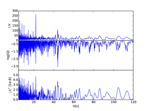
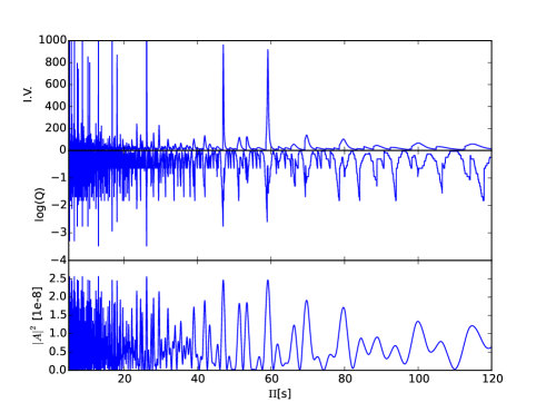
where is the Brunt-Väisälä frequency. In principle, the asymptotic period spacing or the average of the computed period spacings calculated from a grid of models (with different masses and effective temperatures) can be compared with the mean period spacing exhibited by a pulsating WD star, and then a value of the stellar mass can be inferred. The initial step to do so is to obtain (if it exists) a mean period spacing underlying the observed periodicities. We searched for a constant period spacing in the data of the target stars by using the Kolmogorov-Smirnov (K-S; see Kawaler 1988), the Inverse Variance (I-V; see O’Donoghue 1994) and the Fourier Transform (F-T; see Handler et al. 1997) significance tests. In the K-S test, the quantity is defined as the probability that the observed periods are randomly distributed. Thus, any uniform —or at least systematically non-random— period spacing present in the period spectrum of the star under analysis will appear as a minimum in . In the I-V test, a maximum of the inverse variance will indicate the presence of a constant period spacing. Finally, in the F-T test, we calculate the Fourier Transform of a Dirac comb function (created from a set of observed periods), and then we plot the square of the amplitude of the resulting function in terms of the inverse of the frequency. And once again, a maximum in the square of the amplitude will indicate the presence of a constant period spacing.
As we can see in Tables 2 to 10, the number of periods exhibited by all the known ELMV WDs varies from 2 to 7. In particular, because of the few periods exhibited by J1614, J2228, J1738, J1618 and J2139, it is not possible to search for a constant period spacing in these cases. But in the cases of J1840, J1112, J1518 and J1735 we were able to carry this procedure out. Unfortunately, for the cases of J1840 and J1112, we could not estimate any unambiguous constant period spacing, and furthermore, there was not agreement between the significance tests. It might be due to the fact that the periods exhibited by these stars are not fully in the asymptotic regime and/or there are not as many periods as needed to determine a mean period spacing. However, for the cases of J1518 and J1735, as shown in Figs. 2 and 3, respectively, we found clear indication of a constant period spacing for the three independent significance tests for both stars. For J1518, it lies at roughly s, though there is also another possible value at s, both for the three significance tests. However, the latter is too short and probably represents the harmonic of the main period spacing (). In addition, a period separation of s is not likely to be the asymptotic period spacing because the resulting stellar mass would be prohibitively high (Córsico & Althaus 2014a). So, we assume that the period spacing associated with J1518 is s. In the case of J1735, there is a possible value for the period spacing at s but once again, as already mentioned, this value is too short and we discard it. We can also see that there are two other possibilities at s and s, the latter being a more expectable value for the period spacing, according to the asymptotic predictions. So, we adopt s as the period spacing for this star.
3.2 Determination of the stellar mass of J1518 and J1735 from the observed period spacing
In this section, we aim to estimate the masses of J1518 and J1735 by comparing the average of the computed period spacings () for our grid of models with the observed period spacing () determined in the previous Section for each star. We warn that this approach has an issue: the period spacing in this type of stars could be sensitive also on the thickness of the outer H envelope in addition to the stellar mass (Tassoul et al. 1990; Fontaine & Brassard 2008). We defer to a future publication a full exploration of this dependence.
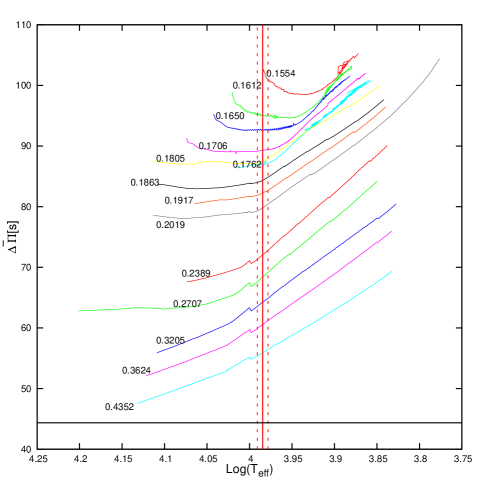
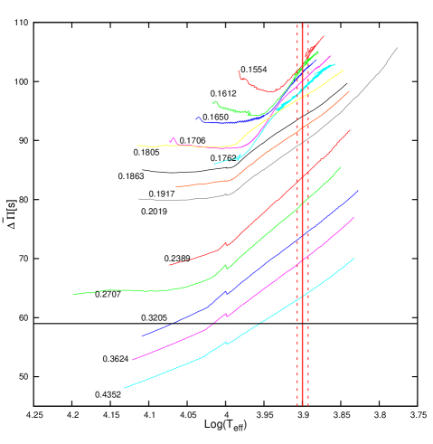
The average of the computed period spacings is assessed as , where the “forward” period spacing is defined as ( being the radial order) and is the number of theoretical periods within the range of the periods observed in the target star. For J1518, s, while for J1735, s.
In Fig. 4 we show the run of the average of the computed period spacings () for J1518 in terms of the logarithm of the effective temperature for our ELM WD evolutionary sequences, along with the observed period spacing for J1518. As can be seen from the Figure, the smaller the values of , the greater the stellar mass. In this case, it clearly shows that such a low value (s) of the observed period spacing would lead to a stellar mass greater than , which is higher than expected for this type of stars. Hence, this analysis does not seem to lead to a proper value of the mass for J1518. It might be due to the fact that this star is not pulsating in the asymptotic regime (see Córsico & Althaus 2014a).
In Fig. 5 we show the run of the average of the
computed period spacings () for J1735 in terms of the
logarithm of the effective temperature for our ELM WD evolutionary
sequences, along with the observed period spacing for J1735. Once
again, the value we obtain for the stellar mass is higher than
expected (), even though this star may be
pulsating in the asymptotic regime. Alternatively, if the value we
have obtained for the observed period spacing is real, in the sense
that it can be associated with the behaviour of high-radial order
modes, then it would indicate that this star has a mass somewhat
larger than , and that their spectroscopic
parameters () could be wrong.
In the next Section we shall follow another approach to estimate the stellar mass and other features of all the known ELMVs, through the search of theoretical models that best fit the individual observed periods. The advantage of this procedure is that, once we have chosen a model, we have access to information of the star otherwise very difficult (if not impossible) to know by any other method.
3.3 Constraints from the individual observed periods: searching for the best-fit model
In this approach we search for a pulsation model that best matches the individual pulsation periods of a given star under study. The goodness of the match between the theoretical pulsation periods () and the observed individual periods () is measured by means of a merit function defined as:
| (2) |
where is the number of observed periods. The ELM model that shows the lowest value of , if exists, is adopted as the “best-fit model”. We assess the function for stellar masses of , , , , , , , , , , , , , and . For the effective temperature we also cover a wide range: K.
We have carried out asteroseismological fits for all the known ELMV WD stars. This is the first time that this procedure is used for this type of stars. We start our analysis assuming that all of the observed periods correspond to modes associated with , and considering the set of observed periods, , of each star to compute the quality function given by Eq. (2). Next, we considered the case in which all of the observed periods correspond to modes associated with , and finally, we considered the case of a mix of modes associated with and . In the case of J1112, we performed a more detailed analysis. For this star we worked with two different sets of observed periods. On the one hand, the five longest periods, for which we carried out the analysis previously mentioned. On the other hand, we adopted the whole set of periods (seven) and explored the possibility that they correspond to a mix of and modes with , and also we considered the case in which the observed periods correspond to radial () and and modes ().
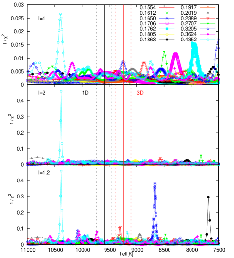
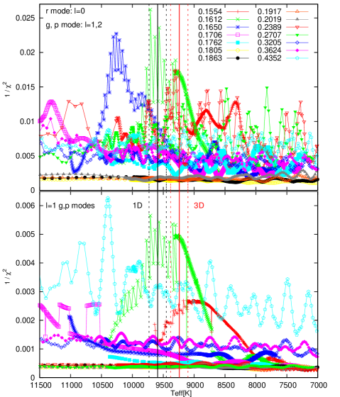
Figs. 6 to 15 show the quantity in terms of the effective temperature for different stellar masses, for each known ELMV, taking into account the corresponding set of observed periods. We also include the effective temperatures and their uncertainties for the 1D (dark gray vertical lines) and 3D model atmospheres (red vertical lines) determinations. As mentioned before, the goodness of the match between the theoretical and the observed periods is measured by the value of : the better the period match, the lower the value of —in the figures, the greater the value of . In some cases, there is a single maximum and we adopt that model as the asteroseismological solution for that star. Sometimes, there are multiple possible solutions, and we need to employ some external constraint in order to choose one. Generally, the constraint is the uncertainty in the effective temperature, given by the spectroscopy. In some cases, when there are still multiple possible solutions, we choose the model with a mass as close as possible to the mass given by the spectroscopic determinations. It is important to mention that, as it is more likely to observe than modes (due to geometric cancellation effects which become stronger with higher values of ; see Dziembowski 1977), we will usually choose, when possible, the asteroseismological solutions that fit to observed periods with a larger number of modes.
3.3.1 The case of J1840
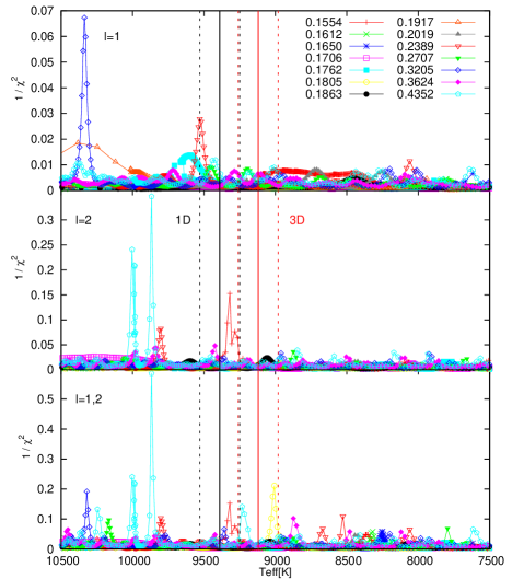
In Fig. 6, the match between the theoretical and the five observed periods of J1840, assuming they are associated with modes, for the cases of (top panel), (middle panel) and (bottom panel), is shown. The case is only depicted for the seek of completeness, since we do not expect that a pulsating star can exhibit all the periods associated to and none of them corresponding to , due to geometric cancellation arguments (see above). For the case, the upper panel shows that there is more than one solution. In particular, the absolute maximum (the best solution) lies at a very higher effective temperature than that allowed by both spectroscopic determinations. The second best solution lies within the range of allowed for the 1D model atmosphere (K), so we may adopt this model because it represents a good period fit. It corresponds to a mass of at K. For the case, once again there is no a single solution, and the best period fit has a very high value of . In the ranges of allowed , we can see that there is no unambiguous asteroseismological model. However, we may adopt the solution given for the model with at K, which is the best fit in the range of allowed for the 3D model atmosphere (K).
In order to know how good the agreement of theoretical and observed periods is, we can compare them by computing the absolute period differences . The results for J1840 are shown in Table 11, for the case of . Column 6 of Table 11 shows the value of the linear nonadiabatic growth rate (), defined as (, where and are the real and the imaginary part, respectively, of the complex eigenfrequency , computed with the nonadiabatic version of the LP-PUL pulsation code (Córsico et al. 2006; Córsico & Althaus 2016). A value of () implies an unstable (stable) mode (see column 6 of Table 11). For the case of the results are shown in Table 12.
Considering that the period fit of the case is better, since it has a larger value of than the solution of the case, and the mass of this model () is in line with the spectroscopic masses determined for this star ( and ), we adopt the model with and K as the asteroseismological solution for J1840, which has a value of in agreement with the spectroscopy (for the 3D model), even though this model has a larger number of than modes. Note that most of the periods of this model correspond to pulsationally unstable modes.
| [s] | [s] | [s] | Remark | |||
|---|---|---|---|---|---|---|
| 1 | unstable | |||||
| 1 | unstable | |||||
| 1 | unstable | |||||
| 1 | unstable | |||||
| 1 | unstable |
| [s] | [s] | [s] | Remark | |||
|---|---|---|---|---|---|---|
| unstable | ||||||
| unstable | ||||||
| unstable | ||||||
| stable | ||||||
| unstable |
3.3.2 The case of J1112
Due to the presence of the two short periods at s and s in the pulsation spectrum of J1112, which are probably associated with or radial modes, we divided the analysis for this star into two parts: on the one hand, we considered the five longest observed periods, assuming that they are all associated with , or a mix of and modes.On the other hand, we considered the whole set of periods (seven), considering firstly, that they are associated with a mix of and modes111We have also explored a possible combination of and modes with and , but we have not obtained significantly different results., and secondly, with a mix of and modes with and , and also radial modes (). At this point, it is worth mentioning that the reality of these two short periods are not definitively confirmed, as claimed by Hermes et al. (2013b). Thus, these separated analyses are worth doing.
In Fig. 7 we show the match between the theoretical and the five longest observed periods of J1112, assuming they are associated with modes, for the cases of (top panel), (middle panel, shown for completeness) and (bottom panel). In the case of , we can see that the absolute maximum is at a very high effective temperature, and there are also many other solutions for low values of . Within the range of allowed for the 3D model atmosphere analysis (K), there may be a solution for the model with at K. We compare the observed and the theoretical periods as we did for the previous star, and the results are displayed in Table 13. If we consider the case of , there are multiple local maxima which are either too hot or too cold in comparison with the allowed values of . Nevertheless, there may be a possible solution within the range of allowed (for the 3D model), for the case of at K. In Table 14 we show the comparison between the observed and the theoretical periods for this model.
| [s] | [s] | [s] | Remark | |||
|---|---|---|---|---|---|---|
| 1 | unstable | |||||
| 1 | unstable | |||||
| 1 | unstable | |||||
| 1 | unstable | |||||
| 1 | unstable |
| [s] | [s] | [s] | Remark | |||
|---|---|---|---|---|---|---|
| unstable | ||||||
| unstable | ||||||
| unstable | ||||||
| unstable | ||||||
| unstable |
Next, we considered the case in which the whole set of observed periods (seven) corresponds to and modes with , and also, the case in which it corresponds to radial () and and modes (). The results are shown in Fig. 8. For the case of the mix of and modes with = 1 (bottom panel), the absolute maximum lies at a high value of and there is no unambiguous solution in the allowed ranges of . However, there may be one possible solution for , that lies in the allowed range of for the 1D model (K). In a more complete analysis, considering the mix of radial () and and modes (), we find that the absolute maximum is at the same model and it represents a better match because it has a larger value of , as shown in the top panel of Fig.8. It is the best period fit for this case, and corresponds to at K. Hence, this represents a very good solution for the case of the whole set of periods. Once again, we show the comparison between the observed and the theoretical periods in Table 15. We can see from this Table that one of the short periods may be associated with a mode (with ) and the other one, with a radial mode ().
Considering all the results from this analysis, we may conclude that the best solution corresponds to the model with and K, which is quite in line with the spectroscopic masses determined for this star ( and ) and also, in line with the given by the spectroscopy (for the 1D model). Unfortunately, our nonadiabatic computations (see Table 15) predict that all the modes of this possible solution are pulsationally stable, forcing us to discard this solution. If we consider this and ignore the two shortest periods of this star, we could adopt the solution found with a mass of and K (see Table 14), although this value of the stellar mass is not in such good agreement with the masses resulting from the spectroscopy. Note, however, that all the periods of this model are associated with pulsationally unstable modes. Finally, the fact that we are not able to find an asteroseismological model having unstable modes with periods that fit the seven periods observed in J1112 (including the shortest ones) could be indicating that the periods at s and s reported by Hermes et al. (2013b) could not be real. This calls for the need of further photometric work on this star.
| [s] | [s] | [s] | Remark | |||||
|---|---|---|---|---|---|---|---|---|
| radial | ||||||||
| — | — | stable | ||||||
| — | — | stable | ||||||
| — | — | stable | ||||||
| — | — | stable | ||||||
| — | — | stable | ||||||
| — | — | stable | ||||||
| — | — | stable |
3.3.3 The case of J1518
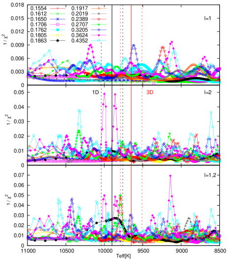
In Fig. 9 we show the match between the theoretical periods and the seven observed periods of J1518 assuming they are associated with modes, for the cases of (top panel), (middle panel) and (bottom panel). In the case, we see multiple local maxima. However, in the range of allowed given by the 3D model atmosphere calculations (K), there is a possible solution that may be chosen as a representative model for J1518. This corresponds to at K. In Table 16 we compare the theoretical and the observed periods for this model. For the case of , the best period fit lies at a very low , and there are multiple local maxima within the ranges of allowed . However, there is a possible solution characterized by and K which, although not so clear in the Figure, is the best period fit that lies within the ranges of allowed (K and K). We present in Table 17 the comparison between the observed and the theoretical periods for this case.
Considering that the solution for the case implies a much better fit (a larger value of ) than the one for the case, we may adopt the model with and K as the asteroseismological solution for this star, which is in line with the given by the spectroscopy. Moreover, most of the periods of the adopted model are associated with pulsationally unstable modes. It is necessary to stress, however, that none of the solutions found are in good agreement with the masses resulting from the spectroscopic determinations ( and ).
| [s] | [s] | [s] | Remark | |||
|---|---|---|---|---|---|---|
| 1 | unstable | |||||
| 1 | unstable | |||||
| 1 | unstable | |||||
| 1 | unstable | |||||
| 1 | unstable | |||||
| 1 | unstable | |||||
| 1 | unstable |
| [s] | [s] | [s] | Remark | |||
|---|---|---|---|---|---|---|
| unstable | ||||||
| unstable | ||||||
| unstable | ||||||
| unstable | ||||||
| unstable | ||||||
| stable | ||||||
| unstable |
3.3.4 The case of J1614
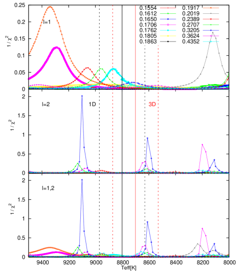
In Fig. 10 we depict the match between the theoretical and the two observed periods of J1614, assuming they are associated with modes, for the cases of (top panel), (middle panel) and (bottom panel). It is worth mentioning in advance that this period fit will not be robust because this star only shows two independent periods.
In the case of , we can see that there is no unambiguous solution, and the best solutions are located beyond the ranges of allowed . However, we may choose the model with and K that lies within the ranges of allowed (K and K), and also has a mass value consistent with the spectroscopic determinations. In Table 18 we show the comparison between the observed and the theoretical periods for this model. In the case of , the best fit is located at a high value of , but the second best fit lies within the range of allowed (for the 3D model). It is characterized by , at K. However, as can be seen in Table 19, the comparison between the observed and the theoretical periods shows that both periods are associated with , which is not usually the case because, as already stated, it is more likely to observe periods associated with than . Hence, the asteroseismological model we adopt corresponds to the case of , with and K, with a mass in line with the spectroscopic determinations ( and ) and a in agreement with the spectroscopy. Finally, as can be seen from Table 18, both periods are associated with pulsationally unstable modes.
| [s] | [s] | [s] | Remark | |||
|---|---|---|---|---|---|---|
| 1 | unstable | |||||
| 1 | unstable |
| [s] | [s] | [s] | Remark | |||
|---|---|---|---|---|---|---|
| unstable | ||||||
| unstable |
3.3.5 The case of J2228
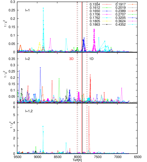
In Fig. 11 we can see the match between the theoretical and the three observed periods of J2228, assuming they are associated with modes, for the cases of (top panel), (middle panel) and (bottom panel). In the case of , we can see that there are multiple possible solutions and that the best fit solution is located at a high value of . Within the ranges of allowed (K and K), there is a possible solution for the model with at K. In Table 20 we show the comparison between the observed and the theoretical periods for this case. In the case of , the absolute maximum lies very close to the ranges of allowed . It corresponds to the model with at K. In Table 21 we display the comparison between the observed and the theoretical periods for this model.
Since the solution for the case of ( and K) implies a much better period fit than the solution for the case of , since it lies at a value of almost compatible with the values given by spectroscopy, and because its mass is in line with the spectroscopic determinations for the mass ( and ), we adopt this model as the asteroseismological solution for J2228. According to our nonadiabatic computations (Table 21), most of the periods of the adopted model are associated with pulsationally unstable modes.
| [s] | [s] | [s] | Remark | |||
|---|---|---|---|---|---|---|
| 1 | unstable | |||||
| 1 | unstable | |||||
| 1 | stable |
| [s] | [s] | [s] | Remark | |||
|---|---|---|---|---|---|---|
| unstable | ||||||
| stable | ||||||
| unstable |
3.3.6 The case of J1738
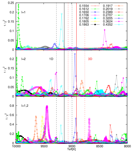
In Fig. 12 we depict the match between the theoretical and the three observed periods of J1738, assuming they are associated with modes, for the cases of (top panel), (middle panel) and (bottom panel). In the case of , the best solution lies at a very high value of , but the second best solution lies within the range of allowed (for the 1D atmosphere model determination, K). This solution is characterized by at K, and the comparison between the observed and the theoretical periods is shown in Table 22. In the case of , the absolute maximum is located at a higher effective temperature than the allowed by spectroscopy (K and K, 1D and 3D models, respectively), and there are many other solutions. However, the models with at K and at K are relatively good period fits that lie within the ranges of allowed . When we analyze in detail the period to period fit, we see that the latter (shown in Table 23) may be more realistic due to the fact that more modes are associated with than . The opposite happens with the former, so we may rather choose the solution with though is not the best one.
From this analysis, since the values of for the two possible solutions are not significantly different, and the value of the mass is the same for both of them, but the solution for the case has more periods associated with pulsationally unstable modes, we conclude that this is the best asteroseismological solution, characterized by and K, which is in line with the given by the spectroscopy (for the 1D model atmosphere computations). However, when we compare the mass of this model with the masses from the spectroscopic determinations ( and ) we see that they are not in good agreement. In summary, we cannot find any agreement between the asteroseismological and the spectroscopic results for J1738.
| [s] | [s] | [s] | Remark | |||
|---|---|---|---|---|---|---|
| 1 | unstable | |||||
| 1 | unstable | |||||
| 1 | stable |
| [s] | [s] | [s] | Remark | |||
|---|---|---|---|---|---|---|
| unstable | ||||||
| stable | ||||||
| stable |
3.3.7 The case of J1618
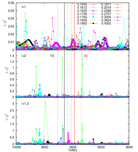
In Fig. 13 we show the match between the theoretical and the three observed periods of J1618, assuming they are associated with modes, for the cases of (top panel), (middle panel) and (bottom panel). In the case of , we can see that there is no unambiguous solution. Within the range of allowed for the 1D model (K), there is a possible solution for the model with at K, and in the range of allowed for the 3D model (K) there is another possible solution for the model characterized by at K. The latter may be more suitable as a solution because its mass is in line with the spectroscopic determinations of the stellar mass (and in comparison, the period fit for the other solution is not significantly better). In Table 24 we show the comparison between the observed and the theoretical periods for the model with . The panel for the case of a mix of modes with shows an absolute maximum for a higher value of than allowed, and does not show any unambiguous solution in the ranges of allowed . However, there is a possible solution characterized by at K because despite not being the best period fit in the ranges of allowed , it corresponds to modes associated both with and (and not only , see Table 25) and also the mass is quite in line with the mass of the spectroscopic determination.
Although the solution for the case () has a mass slightly closer to the masses from the spectroscopic determinations for J1618 ( and ) than the solution for the case (), if we consider the fact that the latter is a better match between the observed and the theoretical periods, and also that this value of the stellar mass is more realistic for this type of stars, we conclude that the model with and K, is a more suitable solution. Also, the is in line with the spectroscopy. Hence, this is the model we adopt for J1618. Note that all of the periods of the adopted model are associated with pulsationally unstable modes.
| [s] | [s] | [s] | Remark | |||
|---|---|---|---|---|---|---|
| 1 | unstable | |||||
| 1 | unstable | |||||
| 1 | stable |
| [s] | [s] | [s] | Remark | |||
|---|---|---|---|---|---|---|
| unstable | ||||||
| unstable | ||||||
| unstable |
3.3.8 The case of J1735
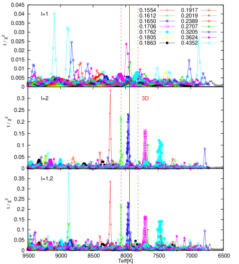
In Fig. 14 we plot the match between the theoretical and the four observed periods of J1735 assuming they are associated with modes, for the cases of (top panel), (middle panel) and (bottom panel). In the case, we can see that there are multiple local maxima that have values of which are either too high or too low in comparison with the range of allowed (K). However, there is a possible solution within that range, corresponding to the model with at K. In Table 26 we show the comparison between the observed and the theoretical periods for the mentioned model. Note, however, that this stellar model that constitutes a possible seismological solution for J1735, has all the modes pulsationally stable. As for the case of , we can see that the best fit models have values of higher than allowed. Although there is a possible solution within the range of allowed for the model characterized by at K, when we compare the observed and the theoretical periods, we find that they are all associated with . Then, the model with that lies at a slightly higher value of than allowed (K), may be a good solution for this case (see Table 27).
Taking into consideration the spectroscopic determination for the mass of J1735, , and comparing the quality of the period fit of the asteroseismological results, we find that the model with and K, is an appropriate solution (with the almost compatible with the spectroscopy) and this is the one we adopt. This model has most of its periods associated with pulsationally unstable modes.
| [s] | [s] | [s] | Remark | |||
|---|---|---|---|---|---|---|
| 1 | stable | |||||
| 1 | stable | |||||
| 1 | stable | |||||
| 1 | stable |
| [s] | [s] | [s] | Remark | |||
|---|---|---|---|---|---|---|
| unstable | ||||||
| unstable | ||||||
| stable | ||||||
| unstable |
3.3.9 The case of J2139
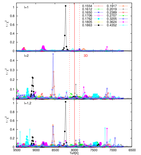
In Fig. 15 we depict the match between the theoretical and the three observed periods of J2139 assuming they are associated with modes, for the cases of (top panel), (middle panel) and (bottom panel). In the first case, we see that the absolute maximum, located at K for a model with , is very close to the range of allowed (K). Then, it represents a good solution. In the case of a mix of modes with , the absolute maximum corresponds to the same model, and the three periods are associated with . There are other possible solutions but they lie far from the range of allowed , and inside that range, the fits are not good. For the model with , we show the comparison between the observed and the theoretical periods in Table 28.
Considering these results, we may adopt the mentioned model, with and K, which although is not quite in line with the spectroscopic result for the mass () and the , is a very good period fit (with all the periods associated with modes), and also has all the periods associated with pulsationally unstable modes.
| [s] | [s] | [s] | Remark | |||
|---|---|---|---|---|---|---|
| 1 | unstable | |||||
| 1 | unstable | |||||
| 1 | unstable |
4 Summary and conclusions
| Star | Period fit | Spectroscopy | |||
| (other works) | |||||
| (radial) | 1D | 3D | |||
| J1840 | 0.2389 | 0.1805 | — | 0.183a | 0.177f |
| J1112 | 0.3205∗ | 0.2389∗ | 0.1612∗∗ | 0.179b | 0.169f |
| J1518 | 0.3205 | 0.2707 | — | 0.220b | 0.197f |
| J1614 | 0.1762 | 0.3205 | — | 0.192c | 0.172f |
| J2228 | 0.1650 | 0.1554 | — | 0.152c | 0.142f |
| J1738 | 0.4352 | 0.4352 | — | 0.181d | 0.172f |
| J1618 | 0.2019 | 0.1706 | — | 0.220e | 0.179f |
| J1735 | 0.3624 | 0.1612 | — | — | 0.142g |
| J2139 | 0.1863 | — | — | — | 0.149g |
Notes: aHermes et al. (2012). ∗ Determined using a subset of the observed periods. ∗∗ Determined using the whole set of the observed periods. bHermes et al. (2013b). cHermes et al. (2013a). dKilic et al. (2015). eBell et al. (2015). f Determined using the corrections for 3D effects by Tremblay et al. (2015). gBell et al. (2017).
In this work, we have presented a detailed asteroseismological study of all the known pulsating ELM WD stars (ELMVs), considering the pulsation spectrum they exhibit and employing the set of evolutionary models of Althaus et al. (2013). This is the fifth paper in a series of works dedicated on pulsating low-mass, He-core WDs (including ELMV WDs). The present paper is devoted to perform the first asteroseismological analysis of all the known ELMV stars. For this purpose we employed some asteroseismological tools. One of them is based on the comparison between the observed period spacing of the star under analysis with the average of the period spacings computed on our grid of models. So firstly, we tried to determine the observed period spacing for each target star, through three independent significance tests. Given that the stars under study exhibit few periods, we could only follow this approach for the cases of the stars showing four periods or more, i.e. J1840, J1112, J1518 and J1735. However, for the first two stars we could not find any unambiguous constant period spacing. In the case of J1518 and J1735, on the other hand, we found a clear indication of a constant period spacing at roughly s and s, respectively, from the three significance tests applied. After comparing these values with the average of the computed period spacings for our grid of models, we found that the resulting stellar masses (greater than in both cases) are higher than expected for this type of stars. In the case of J1518, it may be associated with the fact that this star is not pulsating in the asymptotic regime (Córsico & Althaus 2014a). The case of J1735 is more intriguing because this star seems to be in that regime.
Next, we searched for the best-fit model, i.e. the theoretical model that provides the best match between the individual pulsation periods exhibited by the star and the theoretical pulsation periods. We assessed the function (given by Eq. 2 of Section 3.3) for our complete set of model sequences, covering a wide range in effective temperature ( K). Due to the multiplicity of solutions, we were forced to employ some external constraints (for instance, the uncertainty in the , given by spectroscopy). We assumed that all of the observed periods correspond to g modes and considered them to compute the quality function for each target star. We also considered the (unlikely) case in which all of the observed periods correspond to g modes. Finally, we considered the case of a mix of and g modes. For the particular case of the star J1112, we performed two different analyses. Since the two shortest periods reported for this star are not confirmed (Hermes et al. 2013b), first we carried out a period fit applied to the subset of the five longest periods exhibited by this star considering they are associated with , and a mix of and g modes. Second, for the whole set of seven periods, we explored two possibilities: that all of the observed periods correspond to a mix of and modes (), and also the case in which the observed periods correspond to radial () and and modes (). In Table 29 we show a compilation of the mass determinations for the ELMVs both from spectroscopic (other works) and period-fit results (this work). Considering the obtained results, we found that the seismological mass is in good agreement with the spectroscopic determinations for J1840 (in the case of a mix of g modes), J1614 (for the case of modes), J2228 (for the case of modes), J1618 (for the case of modes), and J1735 (for the case of modes). We consider that there is a good agreement between the seismological and spectroscopic mass when the difference is below the uncertainty of 15%, that is, the typical difference in the mass value derived from independent sets of evolutionary tracks. Then, we conclude that for most of the target stars, the adopted models from the asteroseismological analyses have masses which are in line with the spectroscopic results. At variance with this, for four stars (J1738, J1518, J1112 and J2139) we obtained a larger value of the stellar mass in comparison with the spectroscopic determinations. In particular, gathering together the mass determinations for J1518, we conclude that there is no agreement between the mass given by the spectroscopy ( and ), the mass obtained from the comparison between the observed period spacing and the average of the computed period spacings (which is larger than ), and the mass from the adopted asteroseismological model (). We also mention that, in spite of the fact that we were able to adopt a seismological model for J1735 whose mass () is in line with the spectroscopic determination (), we could not find such agreement for the mass resulting from the comparison between the observed period spacing and the average of the computed period spacings (). Reversing the argument, as this star seems to be in the asymptotic regime, if the value we have obtained for the period spacing of this star were in fact associated with high-radial order modes, it could indicate that the stellar mass is higher than the determined by the spectroscopic and the period-to-period fit analysis, though in that case the star could not be classified as an ELMV WD star. Finally, it is worth mentioning that, in general, the pulsation periods corresponding to the asteroseismological models adopted in this work for the analysed ELMV WDs are pulsationally unstable, according to our nonadiabatic computations. This agreement between the adiabatic and nonadiabatic predictions gives more relevance to our asteroseismological results.
From the results presented in this paper for all the known ELMVs, it is evident once again the power of this approach, since in most of the cases we were able to constrain the value of the stellar mass. Moreover, once a model has been adopted we can access to additional information, as can be seen in Table 30, which is another advantage of asteroseismology. Taking into account these results, four of the stars under analysis (J1840, J1518, J1738 and J2139) are not strictly ELM WD according to our definition previously stated, that is, the progenitors of these stars might have experienced multiple flashes.
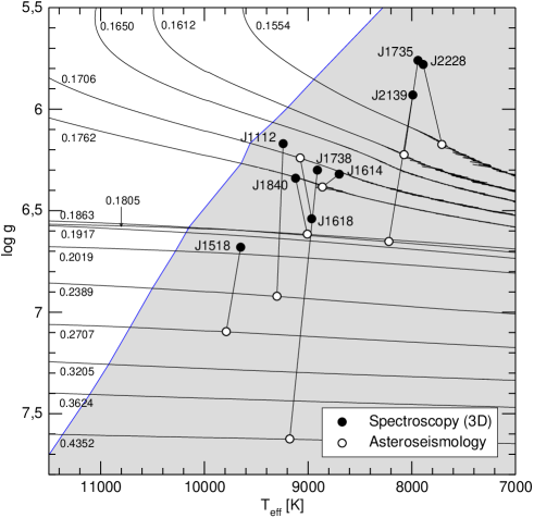
In Fig. 16 we show the location of the nine analysed ELMVs (according to the 3D model-atmosphere parameters) and the corresponding values of and of the asteroseismological models adopted for each star, along with our evolutionary tracks of low mass He-core WDs and the the instability domain of modes computed by Córsico & Althaus (2016). As we mentioned, for five stars we found good agreement between the seismological mass and the spectroscopic one, and for the remaining four stars the agreement is not good. Beyond that, Fig. 16 demonstrates that for eight out of nine stars analyzed, the asteroseismological models are more massive (i.e., they are characterized by higher gravities) in comparison with the spectroscopy results. This systematic trend is also found in the case (not shown) in which the and values derived from calculations of 1D atmospheres are adopted. This trend could be related, in part, to the fact that we are not considering low-mass He-core WD models characterized by outer H envelopes thinner than those predicted by the complete binary evolutionary history of the progenitor stars. Alternatively, it could be an indication that the spectroscopic determinations of and in this class of stars were not proper.
| Star | [K] | [cgs] | |||
|---|---|---|---|---|---|
| J1840 | 9007 | 6.6156 | 0.1805 | -1.4609 | -2.1487 |
| J1112∗ | 9300 | 6.9215 | 0.2389 | -1.5528 | -2.2757 |
| J1518∗ | 9789 | 7.0956 | 0.2707 | -1.6126 | -2.3098 |
| J1614 | 8862 | 6.3832 | 0.1762 | -1.3497 | -1.9547 |
| J2228 | 7710 | 6.1738 | 0.1554 | -1.2725 | -2.0409 |
| J1738∗ | 9177 | 7.6241 | 0.4352 | -1.7746 | -2.7447 |
| J1618 | 9076 | 6.2403 | 0.1706 | -1.2857 | -1.7852 |
| J1735 | 8075 | 6.2241 | 0.1612 | -1.2899 | -1.9957 |
| J2139∗ | 8221 | 6.6515 | 0.1863 | -1.4724 | -2.3279 |
Note: ∗ Solution whose mass is in conflict with the spectroscopic results.
In this paper, we have considered low-mass He-core WDs coming from solar metallicity progenitors, typical of the population of the Galactic Disk. The threshold in the stellar mass value, below which CNO flashes on the early WD cooling branch are not expected to occur, is . If we had adopted progenitors with lower metallicities, representative of the population of the Galactic Halo, the threshold mass limit should be larger (see Serenelli et al. (2002); Nelson et al. (2004); Istrate et al. (2016b). Also, the H envelope of the low-mass WDs should be thicker than those obtained in Althaus et al. (2013) (e.g. Istrate et al. 2016b). So, by assuming that some of the ELMVs studied in this work are actually objects of the Galactic Halo, the asteroseismological analysis should be based on evolutionary models coming from low metallicity progenitors, and therefore the characteristics of the asteroseismological models for each analyzed star could be different to those obtained in this work.
In this study, we have considered low-mass He-core WD models characterized by thick outer H envelopes, consistent with the previous evolution. We are well aware that there are strong uncertainties about the precise value of the thickness of this envelope. We cannot discard that WD models with H envelopes thinner than those characterizing our set of models could result from binary evolution computations that assume different angular-momentum loss prescriptions due to mass loss, different initial mass-ratio, etc, than that adopted in Althaus et al. (2013) (see the detailed works by Istrate 2015; Istrate et al. 2016b). Asteroseismological analyses considering low-mass He-core WD models characterized by thinner outer H envelopes will be the core feature of a future work.
Acknowledgements.
We wish to thank our anonymous referee for the constructive comments and suggestions that greatly improved the original version of the paper. Part of this work was supported by AGENCIA through the Programa de Modernización Tecnológica BID 1728/OC-AR, and by the PIP 112-200801-00940 grant from CONICET. This research made use of NASA Astrophysics Data System.References
- Althaus et al. (2015) Althaus, L. G., Camisassa, M. E., Miller Bertolami, M. M., Córsico, A. H., & García-Berro, E. 2015, A&A, 576, A9
- Althaus et al. (2010) Althaus, L. G., Córsico, A. H., Isern, J., & García-Berro, E. 2010, A&A Rev., 18, 471
- Althaus et al. (2013) Althaus, L. G., Miller Bertolami, M. M., & Córsico, A. H. 2013, A&A, 557, A19
- Althaus et al. (2009) Althaus, L. G., Panei, J. A., Romero, A. D., et al. 2009, A&A, 502, 207
- Althaus et al. (2005) Althaus, L. G., Serenelli, A. M., Panei, J. A., et al. 2005, A&A, 435, 631
- Bell et al. (2017) Bell, K. J., Gianninas, A., Hermes, J. J., et al. 2017, ApJ, 835, 180
- Bell et al. (2015) Bell, K. J., Kepler, S. O., Montgomery, M. H., et al. 2015, in Astronomical Society of the Pacific Conference Series, Vol. 493, 19th European Workshop on White Dwarfs, ed. P. Dufour, P. Bergeron, & G. Fontaine, 217
- Bischoff-Kim et al. (2008) Bischoff-Kim, A., Montgomery, M. H., & Winget, D. E. 2008, ApJ, 675, 1505
- Bognár et al. (2014) Bognár, Z., Paparó, M., Córsico, A. H., Kepler, S. O., & Győrffy, Á. 2014, A&A, 570, A116
- Bognár et al. (2016) Bognár, Z., Paparó, M., Molnár, L., et al. 2016, MNRAS, 461, 4059
- Bradley (1998) Bradley, P. A. 1998, ApJS, 116, 307
- Bradley (2001) Bradley, P. A. 2001, ApJ, 552, 326
- Brassard et al. (1991) Brassard, P., Fontaine, G., Wesemael, F., Kawaler, S. D., & Tassoul, M. 1991, ApJ, 367, 601
- Brickhill (1991) Brickhill, A. J. 1991, MNRAS, 251, 673
- Brown et al. (2016) Brown, W. R., Gianninas, A., Kilic, M., Kenyon, S. J., & Allende Prieto, C. 2016, ApJ, 818, 155
- Brown et al. (2013) Brown, W. R., Kilic, M., Allende Prieto, C., Gianninas, A., & Kenyon, S. J. 2013, ApJ, 769, 66
- Brown et al. (2010) Brown, W. R., Kilic, M., Allende Prieto, C., & Kenyon, S. J. 2010, ApJ, 723, 1072
- Brown et al. (2012) Brown, W. R., Kilic, M., Allende Prieto, C., & Kenyon, S. J. 2012, ApJ, 744, 142
- Brown et al. (2017) Brown, W. R., Kilic, M., & Gianninas, A. 2017, ApJ, 839, 23
- Burgers (1969) Burgers, J. M. 1969, Flow Equations for Composite Gases (New York: Academic Press)
- Calcaferro et al. (2016) Calcaferro, L. M., Córsico, A. H., & Althaus, L. G. 2016, A&A, 589, A40
- Calcaferro et al. (2017) Calcaferro, L. M., Córsico, A. H., & Althaus, L. G. 2017, A&A, 600, A73
- Cassisi et al. (2007) Cassisi, S., Potekhin, A. Y., Pietrinferni, A., Catelan, M., & Salaris, M. 2007, ApJ, 661, 1094
- Castanheira & Kepler (2008) Castanheira, B. G. & Kepler, S. O. 2008, MNRAS, 385, 430
- Castanheira & Kepler (2009) Castanheira, B. G. & Kepler, S. O. 2009, MNRAS, 396, 1709
- Córsico & Althaus (2006) Córsico, A. H. & Althaus, L. G. 2006, A&A, 454, 863
- Córsico & Althaus (2014a) Córsico, A. H. & Althaus, L. G. 2014a, A&A, 569, A106
- Córsico & Althaus (2014b) Córsico, A. H. & Althaus, L. G. 2014b, ApJ, 793, L17
- Córsico & Althaus (2016) Córsico, A. H. & Althaus, L. G. 2016, A&A, 585, A1
- Córsico et al. (2008) Córsico, A. H., Althaus, L. G., Kepler, S. O., Costa, J. E. S., & Miller Bertolami, M. M. 2008, A&A, 478, 869
- Córsico et al. (2006) Córsico, A. H., Althaus, L. G., & Miller Bertolami, M. M. 2006, A&A, 458, 259
- Córsico et al. (2012a) Córsico, A. H., Althaus, L. G., Miller Bertolami, M. M., & Bischoff-Kim, A. 2012a, A&A, 541, A42
- Córsico et al. (2009) Córsico, A. H., Althaus, L. G., Miller Bertolami, M. M., & García-Berro, E. 2009, A&A, 499, 257
- Córsico et al. (2007a) Córsico, A. H., Althaus, L. G., Miller Bertolami, M. M., & Werner, K. 2007a, A&A, 461, 1095
- Córsico et al. (2016) Córsico, A. H., Althaus, L. G., Serenelli, A. M., et al. 2016, A&A, 588, A74
- Córsico et al. (2007b) Córsico, A. H., Miller Bertolami, M. M., Althaus, L. G., Vauclair, G., & Werner, K. 2007b, A&A, 475, 619
- Córsico et al. (2012b) Córsico, A. H., Romero, A. D., Althaus, L. G., & Hermes, J. J. 2012b, A&A, 547, A96
- Corti et al. (2016) Corti, M. A., Kanaan, A., Córsico, A. H., et al. 2016, A&A, 587, L5
- Dziembowski (1977) Dziembowski, W. 1977, Acta Astron., 27, 203
- Dziembowski (1971) Dziembowski, W. A. 1971, Acta Astron., 21, 289
- Fontaine & Brassard (2008) Fontaine, G. & Brassard, P. 2008, PASP, 120, 1043
- Fontaine et al. (2017) Fontaine, G., Istrate, A., Gianninas, A., Brassard, P., & Van Grootel, V. 2017, in Astronomical Society of the Pacific Conference Series, Vol. 509, 20th European White Dwarf Workshop, ed. P.-E. Tremblay, B. Gaensicke, & T. Marsh, 347
- Giammichele et al. (2017a) Giammichele, N., Charpinet, S., Brassard, P., & Fontaine, G. 2017a, A&A, 598, A109
- Giammichele et al. (2017b) Giammichele, N., Charpinet, S., Fontaine, G., & Brassard, P. 2017b, ApJ, 834, 136
- Giammichele et al. (2016) Giammichele, N., Fontaine, G., Brassard, P., & Charpinet, S. 2016, ApJS, 223, 10
- Gianninas et al. (2016) Gianninas, A., Curd, B., Fontaine, G., Brown, W. R., & Kilic, M. 2016, ApJ, 822, L27
- Gianninas et al. (2014a) Gianninas, A., Dufour, P., Kilic, M., et al. 2014a, ApJ, 794, 35
- Gianninas et al. (2014b) Gianninas, A., Hermes, J. J., Brown, W. R., et al. 2014b, ApJ, 781, 104
- Gianninas et al. (2015) Gianninas, A., Kilic, M., Brown, W. R., Canton, P., & Kenyon, S. J. 2015, ApJ, 812, 167
- Haft et al. (1994) Haft, M., Raffelt, G., & Weiss, A. 1994, ApJ, 425, 222
- Handler et al. (1997) Handler, G., Pikall, H., O’Donoghue, D., et al. 1997, MNRAS, 286, 303
- Hermes et al. (2014) Hermes, J. J., Gänsicke, B. T., Koester, D., et al. 2014, MNRAS, 444, 1674
- Hermes et al. (2013a) Hermes, J. J., Montgomery, M. H., Gianninas, A., et al. 2013a, MNRAS, 436, 3573
- Hermes et al. (2013b) Hermes, J. J., Montgomery, M. H., Winget, D. E., et al. 2013b, ApJ, 765, 102
- Hermes et al. (2012) Hermes, J. J., Montgomery, M. H., Winget, D. E., et al. 2012, ApJ, 750, L28
- Iglesias & Rogers (1996) Iglesias, C. A. & Rogers, F. J. 1996, ApJ, 464, 943
- Istrate (2015) Istrate, A. G. 2015, in Astronomical Society of the Pacific Conference Series, Vol. 493, 19th European Workshop on White Dwarfs, ed. P. Dufour, P. Bergeron, & G. Fontaine, 487
- Istrate et al. (2016a) Istrate, A. G., Fontaine, G., Gianninas, A., et al. 2016a, A&A, 595, L12
- Istrate et al. (2016b) Istrate, A. G., Marchant, P., Tauris, T. M., et al. 2016b, A&A, 595, A35
- Itoh et al. (1996) Itoh, N., Hayashi, H., Nishikawa, A., & Kohyama, Y. 1996, ApJS, 102, 411
- Kawaler (1988) Kawaler, S. D. 1988, in IAU Symposium, Vol. 123, Advances in Helio- and Asteroseismology, ed. J. Christensen-Dalsgaard & S. Frandsen, 329
- Kepler et al. (2014) Kepler, S. O., Fraga, L., Winget, D. E., et al. 2014, MNRAS, 442, 2278
- Kepler et al. (2012) Kepler, S. O., Pelisoli, I., Peçanha, V., et al. 2012, ApJ, 757, 177
- Kilic et al. (2011) Kilic, M., Brown, W. R., Allende Prieto, C., et al. 2011, ApJ, 727, 3
- Kilic et al. (2012) Kilic, M., Brown, W. R., Allende Prieto, C., et al. 2012, ApJ, 751, 141
- Kilic et al. (2015) Kilic, M., Hermes, J. J., Gianninas, A., & Brown, W. R. 2015, MNRAS, 446, L26
- Koester et al. (2009) Koester, D., Voss, B., Napiwotzki, R., et al. 2009, A&A, 505, 441
- Magni & Mazzitelli (1979) Magni, G. & Mazzitelli, I. 1979, A&A, 72, 134
- Maxted et al. (2011) Maxted, P. F. L., Anderson, D. R., Burleigh, M. R., et al. 2011, MNRAS, 418, 1156
- Maxted et al. (2014) Maxted, P. F. L., Serenelli, A. M., Marsh, T. R., et al. 2014, MNRAS, 444, 208
- Maxted et al. (2013) Maxted, P. F. L., Serenelli, A. M., Miglio, A., et al. 2013, Nature, 498, 463
- Nelson et al. (2004) Nelson, L. A., Dubeau, E., & MacCannell, K. A. 2004, ApJ, 616, 1124
- O’Donoghue (1994) O’Donoghue, D. 1994, MNRAS, 270, 222
- Paparó et al. (2013) Paparó, M., Bognár, Z., Plachy, E., Molnár, L., & Bradley, P. A. 2013, MNRAS, 432, 598
- Pech & Vauclair (2006) Pech, D. & Vauclair, G. 2006, A&A, 453, 219
- Pech et al. (2006) Pech, D., Vauclair, G., & Dolez, N. 2006, A&A, 446, 223
- Romero et al. (2012) Romero, A. D., Córsico, A. H., Althaus, L. G., et al. 2012, MNRAS, 420, 1462
- Romero et al. (2013) Romero, A. D., Kepler, S. O., Córsico, A. H., Althaus, L. G., & Fraga, L. 2013, ApJ, 779, 58
- Saio et al. (1983) Saio, H., Winget, D. E., & Robinson, E. L. 1983, ApJ, 265, 982
- Serenelli et al. (2002) Serenelli, A. M., Althaus, L. G., Rohrmann, R. D., & Benvenuto, O. G. 2002, MNRAS, 337, 1091
- Steinfadt et al. (2010) Steinfadt, J. D. R., Bildsten, L., & Arras, P. 2010, ApJ, 718, 441
- Tassoul (1980) Tassoul, M. 1980, ApJS, 43, 469
- Tassoul et al. (1990) Tassoul, M., Fontaine, G., & Winget, D. E. 1990, ApJS, 72, 335
- Tremblay et al. (2015) Tremblay, P.-E., Gianninas, A., Kilic, M., et al. 2015, ApJ, 809, 148
- Unno et al. (1989) Unno, W., Osaki, Y., Ando, H., Saio, H., & Shibahashi, H. 1989, Nonradial oscillations of stars, ed. T. University of Tokyo Press
- Van Grootel et al. (2013) Van Grootel, V., Fontaine, G., Brassard, P., & Dupret, M.-A. 2013, ApJ, 762, 57
- Winget & Kepler (2008) Winget, D. E. & Kepler, S. O. 2008, ARA&A, 46, 157
- Zhang et al. (2016) Zhang, X. B., Fu, J. N., Li, Y., Ren, A. B., & Luo, C. Q. 2016, ApJ, 821, L32