Distribution functions for a family of general-relativistic Hypervirial models in collisionless regime

Henrique Matheus Gauy henmgauy@df.ufscar    Javier Ramos-Caro javier@ufscar.br Departamento de Física, Universidade Federal de São Carlos, São Carlos, 13565-905 SP, Brazil
(March 16, 2024)
Abstract

By considering the Einstein-Vlasov system for static spherically symmetric distributions of matter, we show that configurations with constant anisotropy parameter β𝛽\beta have, necessarily, a distribution function (DF) of the form =l2βξ(ε)superscript𝑙2𝛽𝜉𝜀\mathcal{F}=l^{-2\beta}\xi(\varepsilon), where ε=E/m𝜀𝐸𝑚\varepsilon=E/m and l=L/m𝑙𝐿𝑚l=L/m are the relativistic energy and angular momentum per unit rest mass, respectively. We exploit this result to obtain DFs for the general relativistic extension of the Hypervirial family introduced by Nguyen and Lingam (2013), which Newtonian potential is given by ϕ(r)=ϕo/[1+(r/a)n]1/nitalic-ϕ𝑟subscriptitalic-ϕ𝑜superscriptdelimited-[]1superscript𝑟𝑎𝑛1𝑛\phi(r)=-\phi_{o}/[1+(r/a)^{n}]^{1/n} (a𝑎a and ϕosubscriptitalic-ϕ𝑜\phi_{o} are positive free parameters, n=1,2,𝑛12n=1,2,...). Such DFs can be written in the form n=ln2ξn(ε)subscript𝑛superscript𝑙𝑛2subscript𝜉𝑛𝜀\mathcal{F}_{n}=l^{n-2}\xi_{n}(\varepsilon). For odd n𝑛n, we find that ξnsubscript𝜉𝑛\xi_{n} is a polynomial of order 2n+12𝑛12n+1 in ε𝜀\varepsilon, as in the case of the Hernquist model (n=1𝑛1n=1), for which 1l1(2ε1)(ε1)2proportional-tosubscript1superscript𝑙12𝜀1superscript𝜀12\mathcal{F}_{1}\propto l^{-1}\left(2\varepsilon-1\right)\left(\varepsilon-1\right)^{2}. For even n𝑛n, we can write ξnsubscript𝜉𝑛\xi_{n} in terms of incomplete beta functions (Plummer model, n=2𝑛2n=2, is an example). Since we demand that 00\mathcal{F}\geq 0 throughout the phase space, the particular form of each ξnsubscript𝜉𝑛\xi_{n} leads to restrictions for the values of ϕosubscriptitalic-ϕ𝑜\phi_{o}. For example, for the Hernquist model we find that 0ϕo2/30subscriptitalic-ϕ𝑜230\leq\phi_{o}\leq 2/3, i.e. an upper bounding value less than the one obtained for Nguyen and Lingam (0ϕo10subscriptitalic-ϕ𝑜10\leq\phi_{o}\leq 1), based on energy conditions.

pacs:
04.40.-b, 04.70.Bw, 98.62.Hr

I Introduction

Globular clusters, galactic bulges and dark matter haloes have been usually modeled as many-particle systems endowed by spherical symmetry. Although the Newtonian theory of gravitation is usually chosen as one of the paradigms of galactic dynamics, the idea of formulating these models in the general relativistic realm has been gaining interest in recent decades Lemos and Letelier (1993, 1994); González and Letelier (2000); Semerák and Zácek (2000); Semerák (2002); Zácek and Semerák (2002); Vogt and Letelier (2005); Cooperstock and Tieu (2007); Ramos-Caro and González (2008); Lora-Clavijo et al. (2010); Ramos-Caro et al. (2012); Carrick and Cooperstock (2012); Rodrigues (2012); Herrera-Aguilar and Nucamendi (2014) becoming one of the topical problems in stelar dynamics and relativistic astrophysics.

If one adopts a statistical standpoint to analyze such self-gravitating configurations, it is advisable to perform the description by considering the Einstein-Vlasov system, in order to provide, in a self-consistent fashion, the metric, the energy-momentum tensor and the distribution function (DF). In the context of galactic dynamics, usually based on Newtonian gravity, these theoretical constructions are called as dynamical models: the set composed by DF, potential and density (see Binney and McMillan (2011); Binney (2010) for example). In this paper, adopting the general relativistic paradigm, we also shall call the solutions of the Einstein-Vlasov system as dynamical models.

On one hand, the DF or probability density function, can be considered as a concept involving all the relevant physical information about the system. Once the DF is known we can have access to astrophysical observables as, for example, the projected density and the light-of-sight velocity, provided by photometric and kinematic measurements. On the other hand, the DF is a dynamical entity governed by a kinetic equation which determines the statistical evolution of the configuration. For systems in collisionless regime it obeys the Vlasov equation, sometimes called as collisionless Boltzmann equation. In the case of many-particle self-gravitating systems, the term “collisionless” is devoted to situations where the gravitational encounters are not significant in the evolution. Important examples are galaxies and clusters of galaxies, whose life time is lesser than the corresponding relaxation time. But for smaller systems as stellar clusters, galactic bulges and haloes, encounters might play a significant role in the evolution and the DF is said to obey the Fokker-Planck equation, which contains a collision term characterized by the so-called diffusion coefficients. Usually, they are computed by taking into account an equilibrium DF that is solution of the Vlasov equation.

In other words, the task of describing the evolution of globular clusters in collision regime, starts with the knowledge of the corresponding stationary DF in collisionless regime. Such a DF must determine, in a self-consistent manner, the associated energy-momentum and metric tensors under equilibrium conditions. In this line we will focus the principal subject of the present paper: providing adequate DFs, solutions of Einstein-Vlasov equations, for certain self-gravitating spherically symmetric configurations of astrophysical interest in general relativity. For such purpose, the well known ρ𝜌\rho to f𝑓f approach of Newtonian gravity Plummer (1911); Eddington (1916); Lynden-Bell (1962); Jaffe (1983); Binney and Tremaine (2008); Hernquist (1990); Pedraza et al. (2012), which obtains the DF starting from the potential-density pair, by inversion, can also be used in the General Relativity realm. Here, we will show that for certain spherical distributions this procedure can be performed analytically.

A wide variety of astrophysical configurations can be represented as spherical systems with pressure anisotropy (the so-called anisotropic models), as confirmed by a number of authors in the last three decades Bowers and Liang (1974); Bayin (1982); Singh et al. (2012); Coley and Tupper (1994); Das et al. (2012); Herrera and Santos (1997); Herrera et al. (2012); Corchero (1998); Das and Kloster (2000); Dev and Gleiser (2002); Hernández and Nuñez (2004); Mak and Harko (2003); Herrera et al. (2004); Maharaj and Chaisi (2006, 2006); Herrera et al. (2008); Sharma and Tikekar (2012); Le Delliou et al. (2013); Herrera and Barreto (2013); Sgró et al. (2013); Nguyen and Pedraza (2013); Nguyen and Lingam (2013). They are characterized by an anisotropy parameter β𝛽\beta measuring the quotient between the radial pressure Prsubscript𝑃𝑟P_{r} and the tangential (or azimuthal) pressure Pθsubscript𝑃𝜃P_{\theta}. In particular, for β𝛽\beta constant (i.e. independent of the radial coordinate r𝑟r), it can be proven that the DF is proportional to L2βsuperscript𝐿2𝛽L^{-2\beta} (see section III.2), as in the case of the hypervirial models Nguyen and Lingam (2013), for which β=(2n)/2𝛽2𝑛2\beta=(2-n)/2, with n=1,2,𝑛12n=1,2,..., admitting some cases of interest. For n=1𝑛1n=1 (the Hernquist model), since limL0=subscript𝐿0\lim_{L\rightarrow 0}\mathcal{F}=\infty, radial orbits are much more abundant that closed orbits and we expect most of the matter distribution to be located in the inner region of the system. For n>2𝑛2n>2, the situation is the opposite: the DF increases with L𝐿L, leading to configurations with an overabundance of closed orbits and we do not expect a large mass concentration near the center. The case n=2𝑛2n=2 (Plummer model) is the only isotropic model of this family, where the mass distribution tends to be homogeneous. These features, along with the interesting property of satisfy the virial theorem locally, makes the hipervirial family a set of models appropriate to represent galaxies and dark matter halos, from both a Newtonian Evans and An (2005) and relativistic Nguyen and Pedraza (2013); Nguyen and Lingam (2013) point of view.

Apart from the characteristics mentioned above, the relativistic hypervirial models introduced by Nguyen and Lingam Nguyen and Lingam (2013) have the remarkable property of having the same constant anisotropy parameter as their Newtonian counterparts. Here we will exploit this fact to derive analytical expressions for the associated general-relativistic DFs determining the energy-momentum tensor and other basic settings making such models physically realizable configurations. In particular, it is worth mentioning that the requirement that the DFs be positive leads to diminish the upper bounds of the free parameters (see section IV), compared with the ones obtained from energy conditions Nguyen and Lingam (2013). In this sense, the requirement that the DFs be positive can be interpreted as a statement more fundamental than the imposition of energy conditions (an interesting analysis can also be found in Andréasson (2011)).

The paper is organized as follows: In Sec. II we comment some general features of the relativistic extension of Hernquist solution, focusing on the requirements that must hold to obtain physically realizable configurations, from the perspective of energy conditions. We will show that they impose an upper bound of 4/3434/3 for the positive free parameter ϕosubscriptitalic-ϕ𝑜\phi_{o}. However this upper limit decreases to 2/3232/3 with the knowledge of the DF (Sec. IV). In Sec. III we present a derivation of the self-gravitation equations (i.e. the Einstein-Vlasov system) for static, spherically symmetric distributions, in order to set the basis for the derivation of distribution functions, which is performed in Secs. IV (for the Hernquist solution) and V (for the Hypervirial family).

Finally, some words on notation. Throughout the paper we use natural units, c=1𝑐1c=1, where c𝑐c is the speed of light. Greek indices μ,ν𝜇𝜈\mu,\nu run from 00 to 333. When using isotropic coordinates (t,r,θ,ψ)𝑡𝑟𝜃𝜓(t,r,\theta,\psi) we introduce the following associations for indices: 0t0𝑡0\rightarrow t, 1r1𝑟1\rightarrow r, 2θ2𝜃2\rightarrow\theta and 3ψ3𝜓3\rightarrow\psi. Thus the symbol Trrsuperscript𝑇𝑟𝑟T^{rr} will denote T11superscript𝑇11T^{11}, as well as P0subscript𝑃0P_{0} equals to Ptsubscript𝑃𝑡P_{t}, for example.

II A General-relativistic version for the Hernquist model

The general static isotropic metric, in isotropic coordinates (t,r,θ,ψ)𝑡𝑟𝜃𝜓(t,r,\theta,\psi), can be written as Weinberg (1972)

ds2=A(r)dt2+B(r)(dr2+r2dθ2+r2sin2θdψ2).dsuperscript𝑠2𝐴𝑟dsuperscript𝑡2𝐵𝑟dsuperscript𝑟2superscript𝑟2dsuperscript𝜃2superscript𝑟2superscript2𝜃dsuperscript𝜓2\mathrm{d}s^{2}=-A(r)\mathrm{d}t^{2}+B(r)\left(\mathrm{d}r^{2}+r^{2}\mathrm{d}\theta^{2}+r^{2}\sin^{2}\theta\mathrm{d}\psi^{2}\right). (1)

Also, it can be expressed as a generalized version of the Schwarzschild metric, by defining

A(r)=[1f(r)1+f(r)]2,B(r)=[1+f(r)]4,formulae-sequence𝐴𝑟superscriptdelimited-[]1𝑓𝑟1𝑓𝑟2𝐵𝑟superscriptdelimited-[]1𝑓𝑟4A(r)=\left[\frac{1-f(r)}{1+f(r)}\right]^{2},\qquad B(r)=\left[1+f(r)\right]^{4}, (2)

in which the special case f=GM/2r𝑓𝐺𝑀2𝑟f=-GM/2r represents the Schwarzschild solution, with a Newtonian limit ϕ=GM/ritalic-ϕ𝐺𝑀𝑟\phi=-GM/r. In general, if one chooses f(r)=ϕ(r)/2𝑓𝑟italic-ϕ𝑟2f(r)=-\phi(r)/2, where ϕ(r)italic-ϕ𝑟\phi(r) is any spherical solution of Poisson equation, it gives rise, in the limit c𝑐c\rightarrow\infty, to a Newtonian potential ϕitalic-ϕ\phi. This fact sketches a simple procedure to construct general relativistic extensions of previously known Newtonian solutions, as shown by several authors Buchdahl (1964); Vogt and Letelier (2005, 2010, 2010); Nguyen and Lingam (2013). Here we first focus on the general relativistic extension of the Hernquist potential, one of the models obtained in Nguyen and Lingam (2013). Then we choose f𝑓f as

f(r)=ϕ(r)2,ϕ(r)=ϕo1+(r/a),formulae-sequence𝑓𝑟italic-ϕ𝑟2italic-ϕ𝑟subscriptitalic-ϕ𝑜1𝑟𝑎f(r)=-\frac{\phi(r)}{2},\qquad\phi(r)=-\frac{\phi_{o}}{1+(r/a)}, (3)

where ϕosubscriptitalic-ϕ𝑜\phi_{o} and a𝑎a are positive parameters representing the maximum value of |ϕ|italic-ϕ|\phi| (at the center of the spherical configuration) and a scaling radius, respectively. Note that this metric describes an asymptotically flat space-time with a Ricci scalar given by

R=4ϕoa(r+a)2[a(ϕo1)r]r[r+a(1ϕo2)][r+a(1+ϕo2)]5,𝑅4subscriptitalic-ϕ𝑜𝑎superscript𝑟𝑎2delimited-[]𝑎subscriptitalic-ϕ𝑜1𝑟𝑟delimited-[]𝑟𝑎1subscriptitalic-ϕ𝑜2superscriptdelimited-[]𝑟𝑎1subscriptitalic-ϕ𝑜25R=\frac{4\phi_{o}a(r+a)^{2}[a(\phi_{o}-1)-r]}{r\left[r+a\left(1-\frac{\phi_{o}}{2}\right)\right]\left[r+a\left(1+\frac{\phi_{o}}{2}\right)\right]^{5}},

from which we note that there are two singularities,

(i)r=0,(ii)r=a(ϕo21),formulae-sequence(i)𝑟0(ii)𝑟𝑎subscriptitalic-ϕ𝑜21\mbox{(i)}\>\>\>r=0,\qquad\mbox{(ii)}\>\>\>r=a\left(\frac{\phi_{o}}{2}-1\right), (4)

the second one depending on the free parameters a𝑎a and ϕosubscriptitalic-ϕ𝑜\phi_{o}. It is easy to see that, for ϕo2subscriptitalic-ϕ𝑜2\phi_{o}\leq 2, singularity (ii) disappears. Also, it can be shown that, for 0<ϕo10subscriptitalic-ϕ𝑜10<\phi_{o}\leq 1, we have R<0𝑅0R<0 at any radius (see Fig. 1). In the particular case ϕo=1subscriptitalic-ϕ𝑜1\phi_{o}=1, we find R=4a(r+a)2(r+a/2)1(r+3a/2)5𝑅4𝑎superscript𝑟𝑎2superscript𝑟𝑎21superscript𝑟3𝑎25R=-4a(r+a)^{2}(r+a/2)^{-1}(r+3a/2)^{-5} which means that both singularities, (i) and (ii), disappear. For all other cases, ϕo1subscriptitalic-ϕ𝑜1\phi_{o}\neq 1, we find always a singularity at origin, r=0𝑟0r=0.

Refer to caption
Refer to caption
Refer to caption
Figure 1: We show Ricci scalar for different values of parameter ϕosubscriptitalic-ϕ𝑜\phi_{o}. In particular we plot R~=(a3/4ϕo)R~𝑅superscript𝑎34subscriptitalic-ϕ𝑜𝑅\tilde{R}=(a^{3}/4\phi_{o})R as a function of r~=r/a~𝑟𝑟𝑎\tilde{r}=r/a. For 0<ϕo10subscriptitalic-ϕ𝑜10<\phi_{o}\leq 1, we have R~<0~𝑅0\tilde{R}<0 (left panel). In the half panel we show R𝑅R for 1<ϕo21subscriptitalic-ϕ𝑜21<\phi_{o}\leq 2, which is positive only near the singularity r=0𝑟0r=0. For ϕo>2subscriptitalic-ϕ𝑜2\phi_{o}>2 we have two singularities and also R𝑅R is negative in a prominent region of its domain.

Energy conditions help us to state the range of values for ϕosubscriptitalic-ϕ𝑜\phi_{o} leading to physically realizable configurations. In order to use such conditions, we need the explicit form of the stress-energy tensor, which can be determined via Einstein field equations. We find that the non vanishing components of the stress-energy tensor can be written in terms of f𝑓f:

Ttt=4f3πGϕo2ar(1+f)3(1f)2,superscript𝑇𝑡𝑡4superscript𝑓3𝜋𝐺superscriptsubscriptitalic-ϕ𝑜2𝑎𝑟superscript1𝑓3superscript1𝑓2\displaystyle T^{tt}=\frac{4f^{3}}{\pi G{\phi_{o}}^{2}ar(1+f)^{3}(1-f)^{2}}, (5)
Trr=2f4πGϕo2ar(1+f)9(1f),superscript𝑇𝑟𝑟2superscript𝑓4𝜋𝐺superscriptsubscriptitalic-ϕ𝑜2𝑎𝑟superscript1𝑓91𝑓\displaystyle T^{rr}=\frac{2f^{4}}{\pi G{\phi_{o}}^{2}ar(1+f)^{9}(1-f)}, (6)
Tθθ=Tψψsinθ=f4πGϕo2ar3(1+f)9(1f).superscript𝑇𝜃𝜃superscript𝑇𝜓𝜓𝜃superscript𝑓4𝜋𝐺superscriptsubscriptitalic-ϕ𝑜2𝑎superscript𝑟3superscript1𝑓91𝑓\displaystyle T^{\theta\theta}=T^{\psi\psi}\sin\theta=\frac{f^{4}}{\pi G{\phi_{o}}^{2}ar^{3}(1+f)^{9}(1-f)}. (7)

So, it is easy to state that weak energy condition, Ttt0subscriptsuperscript𝑇𝑡𝑡0-{T^{t}}_{t}\geq 0, is satisfied if ϕo0subscriptitalic-ϕ𝑜0\phi_{o}\geq 0. Strong energy condition, T=Ttt+Trr+Tθθ+Tψψ0𝑇subscriptsuperscript𝑇𝑡𝑡subscriptsuperscript𝑇𝑟𝑟subscriptsuperscript𝑇𝜃𝜃subscriptsuperscript𝑇𝜓𝜓0T=-{T^{t}}_{t}+{T^{r}}_{r}+{T^{\theta}}_{\theta}+{T^{\psi}}_{\psi}\geq 0, leads to

4f3(1+f)5(1f)0,4superscript𝑓3superscript1𝑓51𝑓0\frac{4f^{3}}{(1+f)^{5}(1-f)}\geq 0,

which requires that 0ϕo20subscriptitalic-ϕ𝑜20\leq\phi_{o}\leq 2. Dominant energy condition, given by

|TrrTtt|1,|TθθTtt|1,|TψψTtt|1,formulae-sequencesubscriptsuperscript𝑇𝑟𝑟subscriptsuperscript𝑇𝑡𝑡1formulae-sequencesubscriptsuperscript𝑇𝜃𝜃subscriptsuperscript𝑇𝑡𝑡1subscriptsuperscript𝑇𝜓𝜓subscriptsuperscript𝑇𝑡𝑡1\left|\frac{{T^{r}}_{r}}{{T^{t}}_{t}}\right|\leq 1,\qquad\left|\frac{{T^{\theta}}_{\theta}}{{T^{t}}_{t}}\right|\leq 1,\qquad\left|\frac{{T^{\psi}}_{\psi}}{{T^{t}}_{t}}\right|\leq 1,

is satisfied if ϕo<4/3subscriptitalic-ϕ𝑜43\phi_{o}<4/3. In summary, we have to choose the parameter ϕosubscriptitalic-ϕ𝑜\phi_{o} so that

0ϕo<4/3,0subscriptitalic-ϕ𝑜430\leq\phi_{o}<4/3, (8)

in order to fulfill weak, dominant and strong energy conditions. This means that physically realizable configurations described by (2)-(3) have only one singularity, at the center r=0𝑟0r=0. We shall see, in Sec. IV, by analyzing the behavior of the corresponding distribution function, that we have to choose ϕo2/3subscriptitalic-ϕ𝑜23\phi_{o}\leq 2/3 in order to obtain a DF well defined for r>0𝑟0r>0.

In section V we show that the same procedure can be performed to obtain a general-relativistic extension of the hypervirial potentials, as proven by Nguyen and Ligman in 2013 Nguyen and Lingam (2013).

III Self gravitation equations for static isotropic distributions of matter

In this section we show a detailed derivation of relations which help us to obtain the DF describing the configuration associated with the metric of (1), (2) and (3). At first, we shall deal with functions A(r)𝐴𝑟A(r) and B(r)𝐵𝑟B(r) representing asymptotically flat space-times, in general, and then we consider the particular case in which such functions are given by (2) and (3).

The relation between the stress-energy tensor, Tμνsuperscript𝑇𝜇𝜈T^{\mu\nu}, and the the DF, (xμ,𝒫ν)superscript𝑥𝜇superscript𝒫𝜈\mathcal{F}(x^{\mu},\mathcal{P}^{\nu}) (here 𝒫μ=dxμ/dτsuperscript𝒫𝜇dsuperscript𝑥𝜇d𝜏\mathcal{P}^{\mu}=\mathrm{d}x^{\mu}/\mathrm{d}\tau is the 444-momentum vector and τ𝜏\tau is the proper time), associated with a self-gravitating system, is given by

Tμν=𝒫μ𝒫νgd4𝒫superscript𝑇𝜇𝜈superscript𝒫𝜇superscript𝒫𝜈𝑔superscriptd4𝒫{}T^{\mu\nu}=\int\mathcal{P}^{\mu}\mathcal{P}^{\nu}\mathcal{F}\sqrt{-g}\mathrm{d}^{4}\mathcal{P} (9)

where g=det(gμν)𝑔𝑑𝑒𝑡subscript𝑔𝜇𝜈g=det(g_{\mu\nu}) and we choose 𝒫t>0superscript𝒫𝑡0\mathcal{P}^{t}>0. The phase-space domain associated with a particle of rest mass m𝑚m is determined by the shell condition,

gμν𝒫μ𝒫ν=m2,subscript𝑔𝜇𝜈superscript𝒫𝜇superscript𝒫𝜈superscript𝑚2{}g_{\mu\nu}\mathcal{P}^{\mu}\mathcal{P}^{\nu}=-m^{2}, (10)

from which we can express 𝒫tsuperscript𝒫𝑡\mathcal{P}^{t} as a function of the remaining phase-space coordinates: 𝒫t=𝒫t(𝒫i,xμ)superscript𝒫𝑡superscript𝒫𝑡superscript𝒫𝑖superscript𝑥𝜇\mathcal{P}^{t}=\mathcal{P}^{t}(\mathcal{P}^{i},x^{\mu}). Additionally, neglecting the effect of gravitational encounters in the system, we demand that \mathcal{F} must satisfy the collisionless Boltzmann equation Cercignani and Kremer (2002),

𝒫μxμΓμνλ𝒫μ𝒫ν𝒫λ=0.superscript𝒫𝜇superscript𝑥𝜇subscriptsuperscriptΓ𝜆𝜇𝜈superscript𝒫𝜇superscript𝒫𝜈superscript𝒫𝜆0{}\mathcal{P}^{\mu}\dfrac{\partial\mathcal{F}}{\partial x^{\mu}}-\Gamma^{\lambda}_{\mu\nu}\mathcal{P}^{\mu}\mathcal{P}^{\nu}\dfrac{\partial\mathcal{F}}{\partial\mathcal{P}^{\lambda}}=0. (11)

Such DF, through relation (9) and the Einstein field equations, RμνgμνR/2=8πGTμνsubscript𝑅𝜇𝜈subscript𝑔𝜇𝜈𝑅28𝜋𝐺subscript𝑇𝜇𝜈R_{\mu\nu}-g_{\mu\nu}R/2=-8\pi GT_{\mu\nu}, determines the space-time geometry by the set of relations

Rgμν2Rμν=16πG𝒫μ𝒫νgd4𝒫,𝑅superscript𝑔𝜇𝜈2superscript𝑅𝜇𝜈16𝜋𝐺superscript𝒫𝜇superscript𝒫𝜈𝑔superscriptd4𝒫{}Rg^{\mu\nu}-2R^{\mu\nu}=16\pi G\int\mathcal{P}^{\mu}\mathcal{P}^{\nu}\mathcal{F}\sqrt{-g}\mathrm{d}^{4}\mathcal{P}, (12)

which we denote here as the self-gravitation equations, in the sense that they define, in a self-consistent fashion (obeying simultaneously Einstein’s equations and collisionless Boltzmann equation, or, equivalently, the Einstein-Vlasov system), the evolution of the system.

Relation (11) is equivalent to demand that d/dτ=0dd𝜏0\mathrm{d}\mathcal{F}/\mathrm{d}\tau=0 Straumann (2013), i.e. \mathcal{F} can be regarded as an integral of motion. If the system is endowed by spherical symmetry (or cylindrical or any other) the Jeans theorems guarantee that \mathcal{F} can be expressed as a function the other integrals, which, for the spherical case, are the general relativistic extensions of energy E𝐸E and angular momentum 𝐋𝐋\mathbf{L}. In this paper we are focusing on this case.

Motion of free falling test particles in the static isotropic space-time described by (1) have one constant of motion, the rest mass m𝑚m, and three integrals of motion. The first of them, an energy-like integral of motion, is the t𝑡t-component of the covariant 4-momentum vector, 𝒫tsubscript𝒫𝑡\mathcal{P}_{t}. The second one is the azimuthal angular momentum like integral, 𝒫ψsubscript𝒫𝜓\mathcal{P}_{\psi}, and the third one is the general relativistic version of the total angular momentum, 𝒫θ2+𝒫ψ2/sin2θsuperscriptsubscript𝒫𝜃2superscriptsubscript𝒫𝜓2superscript2𝜃\sqrt{\mathcal{P}_{\theta}^{2}+{\mathcal{P}_{\psi}^{2}}/{\sin^{2}\theta}}. For the sake of simplicity, we adopt the notation

𝒫t=E,𝒫ψ=Lz,𝒫θ2+𝒫ψ2sin2θ=L2,formulae-sequencesubscript𝒫𝑡𝐸formulae-sequencesubscript𝒫𝜓subscript𝐿𝑧superscriptsubscript𝒫𝜃2superscriptsubscript𝒫𝜓2superscript2𝜃superscript𝐿2\mathcal{P}_{t}=-E,\qquad\mathcal{P}_{\psi}=L_{z},\qquad\mathcal{P}_{\theta}^{2}+\frac{\mathcal{P}_{\psi}^{2}}{\sin^{2}\theta}=L^{2}, (13)

and equations of motion for a free falling test particle can be cast as

mdtdτ=𝒫t=EA(r),𝑚𝑑𝑡𝑑𝜏superscript𝒫𝑡𝐸𝐴𝑟\displaystyle m\frac{dt}{d\tau}=\mathcal{P}^{t}=\frac{E}{A(r)},\qquad\qquad\qquad\qquad\qquad\qquad\>\>\>\>\> (14a)
mdψdτ=𝒫ψ=Lzr2B(r)sin2θ,𝑚𝑑𝜓𝑑𝜏superscript𝒫𝜓subscript𝐿𝑧superscript𝑟2𝐵𝑟superscript2𝜃\displaystyle m\frac{d\psi}{d\tau}=\mathcal{P}^{\psi}=\frac{L_{z}}{r^{2}B(r)\sin^{2}\theta},\qquad\qquad\qquad\qquad\>\>\>\>\> (14b)
mdθdτ=𝒫θ=±1r2B(r)L2Lz2sin2θ,𝑚𝑑𝜃𝑑𝜏superscript𝒫𝜃plus-or-minus1superscript𝑟2𝐵𝑟superscript𝐿2superscriptsubscript𝐿𝑧2superscript2𝜃\displaystyle m\frac{d\theta}{d\tau}=\mathcal{P}^{\theta}=\pm\frac{1}{r^{2}B(r)}\sqrt{L^{2}-\frac{L_{z}^{2}}{\sin^{2}\theta}},\qquad\qquad\>\>\>\>\> (14c)
mdrdτ=𝒫r=±E2A(r)B(r)L2r2B2(r)m2B(r),𝑚𝑑𝑟𝑑𝜏superscript𝒫𝑟plus-or-minussuperscript𝐸2𝐴𝑟𝐵𝑟superscript𝐿2superscript𝑟2superscript𝐵2𝑟superscript𝑚2𝐵𝑟\displaystyle m\frac{dr}{d\tau}=\mathcal{P}^{r}=\pm\sqrt{\frac{E^{2}}{A(r)B(r)}-\frac{L^{2}}{r^{2}B^{2}(r)}-\frac{m^{2}}{B(r)}},\>\>\>\> (14d)

remembering that phase space coordinates are constrained by the shell condition. Thus, equations (10) and (14) will be the base for constructing the distribution function.

III.1 The self-gravitation equations

Since gμνsubscript𝑔𝜇𝜈g_{\mu\nu} does not depend on 4-momentum, equation (9) can be written as

Tμν=g𝒫μ𝒫νd4𝒫,superscript𝑇𝜇𝜈𝑔superscript𝒫𝜇superscript𝒫𝜈superscriptd4𝒫T^{\mu\nu}=\sqrt{-g}\int\mathcal{P}^{\mu}\mathcal{P}^{\nu}\mathcal{F}\mathrm{d}^{4}\mathcal{P},

where the integral is defined in all the phase space domain where >00\mathcal{F}>0. Since we are dealing with a DF that is function of the integrals of motion, E𝐸E, Lzsubscript𝐿𝑧L_{z}, L𝐿L and m𝑚m (which, through the shell condition (10), can be interpreted as an integral of motion), it is convenient to make a transformation from coordinates (𝒫t,𝒫r,𝒫θ,𝒫ψ)superscript𝒫𝑡superscript𝒫𝑟superscript𝒫𝜃superscript𝒫𝜓(\mathcal{P}^{t},\mathcal{P}^{r},\mathcal{P}^{\theta},\mathcal{P}^{\psi}) to coordinates (m,E,Lz,L)𝑚𝐸subscript𝐿𝑧𝐿(m,E,L_{z},L). At this point we must be careful with the transformations of 𝒫rsuperscript𝒫𝑟\mathcal{P}^{r} and 𝒫θsuperscript𝒫𝜃\mathcal{P}^{\theta} since, according to (14-c) and (14-d), they have two forms, one for each choosing of sign. Thus, we write

𝒫+r=Lm2(r)L2r2B2(r),𝒫r=𝒫+r,formulae-sequencesubscriptsuperscript𝒫𝑟superscriptsubscript𝐿𝑚2𝑟superscript𝐿2superscript𝑟2superscript𝐵2𝑟subscriptsuperscript𝒫𝑟subscriptsuperscript𝒫𝑟\mathcal{P}^{r}_{+}=\sqrt{\frac{L_{m}^{2}(r)-L^{2}}{r^{2}B^{2}(r)}},\qquad\mathcal{P}^{r}_{-}=-\mathcal{P}^{r}_{+}, (15)

where

Lm(r)=B(r)r2(E2A2(r)m2),subscript𝐿𝑚𝑟𝐵𝑟superscript𝑟2superscript𝐸2superscript𝐴2𝑟superscript𝑚2L_{m}(r)=\sqrt{B(r)r^{2}\left(\frac{E^{2}}{A^{2}(r)}-m^{2}\right)}, (16)

and

𝒫+θ=1r2B(r)L2Lz2sin2θ,𝒫θ=𝒫+θ.formulae-sequencesubscriptsuperscript𝒫𝜃1superscript𝑟2𝐵𝑟superscript𝐿2superscriptsubscript𝐿𝑧2superscript2𝜃subscriptsuperscript𝒫𝜃subscriptsuperscript𝒫𝜃\mathcal{P}^{\theta}_{+}=\frac{1}{r^{2}B(r)}\sqrt{L^{2}-\frac{L_{z}^{2}}{\sin^{2}\theta}},\qquad\mathcal{P}^{\theta}_{-}=-\mathcal{P}^{\theta}_{+}. (17)

Therefore we have to write

Tμν=g[𝒫μ𝒫νd𝒫td𝒫+rd𝒫+θd𝒫ψ+𝒫μ𝒫νd𝒫td𝒫rd𝒫+θd𝒫ψ+𝒫μ𝒫νd𝒫td𝒫+rd𝒫θd𝒫ψ+𝒫μ𝒫νd𝒫td𝒫rd𝒫θd𝒫ψ].superscript𝑇𝜇𝜈𝑔delimited-[]superscript𝒫𝜇superscript𝒫𝜈dsuperscript𝒫𝑡dsubscriptsuperscript𝒫𝑟dsubscriptsuperscript𝒫𝜃dsuperscript𝒫𝜓superscript𝒫𝜇superscript𝒫𝜈differential-dsuperscript𝒫𝑡differential-dsubscriptsuperscript𝒫𝑟differential-dsubscriptsuperscript𝒫𝜃differential-dsuperscript𝒫𝜓superscript𝒫𝜇superscript𝒫𝜈differential-dsuperscript𝒫𝑡differential-dsubscriptsuperscript𝒫𝑟differential-dsubscriptsuperscript𝒫𝜃differential-dsuperscript𝒫𝜓superscript𝒫𝜇superscript𝒫𝜈dsuperscript𝒫𝑡dsubscriptsuperscript𝒫𝑟dsubscriptsuperscript𝒫𝜃dsuperscript𝒫𝜓T^{\mu\nu}=\sqrt{-g}\left[\int\mathcal{P}^{\mu}\mathcal{P}^{\nu}\mathcal{F}\mathrm{d}\mathcal{P}^{t}\mathrm{d}\mathcal{P}^{r}_{+}\mathrm{d}\mathcal{P}^{\theta}_{+}\mathrm{d}\mathcal{P}^{\psi}\right.\\ +\int\mathcal{P}^{\mu}\mathcal{P}^{\nu}\mathcal{F}\mathrm{d}\mathcal{P}^{t}\mathrm{d}\mathcal{P}^{r}_{-}\mathrm{d}\mathcal{P}^{\theta}_{+}\mathrm{d}\mathcal{P}^{\psi}\\ +\int\mathcal{P}^{\mu}\mathcal{P}^{\nu}\mathcal{F}\mathrm{d}\mathcal{P}^{t}\mathrm{d}\mathcal{P}^{r}_{+}\mathrm{d}\mathcal{P}^{\theta}_{-}\mathrm{d}\mathcal{P}^{\psi}\\ +\left.\int\mathcal{P}^{\mu}\mathcal{P}^{\nu}\mathcal{F}\mathrm{d}\mathcal{P}^{t}\mathrm{d}\mathcal{P}^{r}_{-}\mathrm{d}\mathcal{P}^{\theta}_{-}\mathrm{d}\mathcal{P}^{\psi}\right].

In particular, the expression for components Trrsuperscript𝑇𝑟𝑟T^{rr} and Tθθsuperscript𝑇𝜃𝜃T^{\theta\theta} requires a replacement of 𝒫rsuperscript𝒫𝑟\mathcal{P}^{r} and 𝒫θsuperscript𝒫𝜃\mathcal{P}^{\theta} by 𝒫+rsubscriptsuperscript𝒫𝑟\mathcal{P}^{r}_{+}, 𝒫rsubscriptsuperscript𝒫𝑟\mathcal{P}^{r}_{-}, 𝒫+θsubscriptsuperscript𝒫𝜃\mathcal{P}^{\theta}_{+} and//or 𝒫θsubscriptsuperscript𝒫𝜃\mathcal{P}^{\theta}_{-}, according to the variables of integration. For example, in the above expression, the term involving d𝒫+rd𝒫θdsubscriptsuperscript𝒫𝑟dsubscriptsuperscript𝒫𝜃\mathrm{d}\mathcal{P}^{r}_{+}\mathrm{d}\mathcal{P}^{\theta}_{-} requires that we set 𝒫r𝒫+rsuperscript𝒫𝑟subscriptsuperscript𝒫𝑟\mathcal{P}^{r}\rightarrow\mathcal{P}^{r}_{+}, when calculating Trrsuperscript𝑇𝑟𝑟T^{rr}, and it will require 𝒫θ𝒫θsuperscript𝒫𝜃subscriptsuperscript𝒫𝜃\mathcal{P}^{\theta}\rightarrow\mathcal{P}^{\theta}_{-}, when computing Tθθsuperscript𝑇𝜃𝜃T^{\theta\theta}. Note that in all cases, the Jacobian of the transformation is

|(𝒫t,𝒫r,𝒫θ,𝒫ψ)(m,E,L,Lz)|=mL𝒫+r𝒫+θAB4r6sin2θ,superscript𝒫𝑡superscript𝒫𝑟superscript𝒫𝜃superscript𝒫𝜓𝑚𝐸𝐿subscript𝐿𝑧𝑚𝐿subscriptsuperscript𝒫𝑟subscriptsuperscript𝒫𝜃𝐴superscript𝐵4superscript𝑟6superscript2𝜃\left|\dfrac{\partial(\mathcal{P}^{t},\mathcal{P}^{r},\mathcal{P}^{\theta},\mathcal{P}^{\psi})}{\partial(m,E,L,L_{z})}\right|=\frac{mL}{\mathcal{P}^{r}_{+}\mathcal{P}^{\theta}_{+}AB^{4}r^{6}\sin^{2}\theta},

and the domain of integration is given by the relations

{LsinθLzLsinθ0LLm,mAEm,0m.cases𝐿𝜃subscript𝐿𝑧𝐿𝜃otherwise0𝐿subscript𝐿𝑚otherwise𝑚𝐴𝐸𝑚otherwise0𝑚otherwise{}\begin{cases}-L\sin\theta\leq L_{z}\leq L\sin\theta\\ 0\leq L\leq L_{m},\\ m\sqrt{A}\leq E\leq m,\\ 0\leq m\leq\infty.\end{cases} (18)

The bounds for E𝐸E arise from the shell condition and from the escape energy, which can be elucidated from relation (14-d). At r𝑟r\rightarrow\infty we have A=B=1𝐴𝐵1A=B=1, since we are assuming that (1) represents an asymptotically flat metric, and we have

|𝒫r|=E2m2,rformulae-sequencesuperscript𝒫𝑟superscript𝐸2superscript𝑚2𝑟|\mathcal{P}^{r}|=\sqrt{{E^{2}-m^{2}}},\qquad r\rightarrow\infty

Then the escape energy, at r𝑟r\rightarrow\infty, is E=m𝐸𝑚E=m (remember that we chose energy to be positive), corresponding to the value |𝒫r|=0superscript𝒫𝑟0|\mathcal{P}^{r}|=0. Thus, we can state that particles with energy larger than m𝑚m can not belong to the configuration.

It can be shown, from (1), that components of the stress-energy tensor that could be non-vanishing are Tttsuperscript𝑇𝑡𝑡T^{tt}, Trrsuperscript𝑇𝑟𝑟T^{rr}, Tθθsuperscript𝑇𝜃𝜃T^{\theta\theta} and Tψψsuperscript𝑇𝜓𝜓T^{\psi\psi}, whereas the other components vanish in any case (i.e. for an arbitrary DF). This fact can be checked directly from (9), except for the case of Ttψsuperscript𝑇𝑡𝜓T^{t\psi}, which does not vanish trivially. However, since the stress-energy tensor is a function only of radius r𝑟r, it is required that the DF has the form

(m,E,L,Lz)=(m,E,L),𝑚𝐸𝐿subscript𝐿𝑧𝑚𝐸𝐿\mathcal{F}(m,E,L,L_{z})=\mathcal{F}(m,E,L),

leading to Ttψ=0superscript𝑇𝑡𝜓0T^{t\psi}=0 and simplified expressions for the non-vanishing components:

Ttt=4πr2A5/2B3/20mAm0LmE2mL𝒫+rdLdEdm,superscript𝑇𝑡𝑡4𝜋superscript𝑟2superscript𝐴52superscript𝐵32superscriptsubscript0superscriptsubscript𝑚𝐴𝑚subscriptsuperscriptsubscript𝐿𝑚0superscript𝐸2𝑚𝐿subscriptsuperscript𝒫𝑟differential-d𝐿differential-d𝐸differential-d𝑚T^{tt}=\frac{4\pi}{r^{2}A^{5/2}B^{3/2}}\int\limits_{0}^{\infty}\int\limits_{m\sqrt{A}}^{m}\int\limits^{L_{m}}_{0}\frac{E^{2}mL\mathcal{F}}{\mathcal{P}^{r}_{+}}\mathrm{d}L\mathrm{d}E\mathrm{d}m,
Trr=4πr2A1/2B3/20mAm0Lm𝒫+rmLdLdEdm,superscript𝑇𝑟𝑟4𝜋superscript𝑟2superscript𝐴12superscript𝐵32superscriptsubscript0superscriptsubscript𝑚𝐴𝑚subscriptsuperscriptsubscript𝐿𝑚0subscriptsuperscript𝒫𝑟𝑚𝐿differential-d𝐿differential-d𝐸differential-d𝑚T^{rr}=\frac{4\pi}{r^{2}A^{1/2}B^{3/2}}\int\limits_{0}^{\infty}\int\limits_{m\sqrt{A}}^{m}\int\limits^{L_{m}}_{0}{{\mathcal{P}^{r}_{+}}mL\mathcal{F}}\mathrm{d}L\mathrm{d}E\mathrm{d}m,
Tθθ=2πr6A1/2B7/20mAm0LmmL3𝒫+rdLdEdm,superscript𝑇𝜃𝜃2𝜋superscript𝑟6superscript𝐴12superscript𝐵72superscriptsubscript0superscriptsubscript𝑚𝐴𝑚subscriptsuperscriptsubscript𝐿𝑚0𝑚superscript𝐿3subscriptsuperscript𝒫𝑟differential-d𝐿differential-d𝐸differential-d𝑚T^{\theta\theta}=\frac{2\pi}{r^{6}A^{1/2}B^{7/2}}\int\limits_{0}^{\infty}\int\limits_{m\sqrt{A}}^{m}\int\limits^{L_{m}}_{0}\frac{mL^{3}\mathcal{F}}{\mathcal{P}^{r}_{+}}\mathrm{d}L\mathrm{d}E\mathrm{d}m,

and Tψψ=Tθθ/sin2θsuperscript𝑇𝜓𝜓superscript𝑇𝜃𝜃superscript2𝜃T^{\psi\psi}=T^{\theta\theta}/\sin^{2}\theta. In many applications it is common to assume that the mass for every constituent of the system is the same. This lead us to replace (m,E,L)𝑚𝐸𝐿\mathcal{F}(m,E,L) by (E,L)𝐸𝐿\mathcal{F}(E,L), which now satisfies the following simplified form:

Ttt=4πmr2A5/2B3/2mAm0LmE2L(E,L)𝒫+rdLdE,superscript𝑇𝑡𝑡4𝜋𝑚superscript𝑟2superscript𝐴52superscript𝐵32superscriptsubscript𝑚𝐴𝑚subscriptsuperscriptsubscript𝐿𝑚0superscript𝐸2𝐿𝐸𝐿subscriptsuperscript𝒫𝑟differential-d𝐿differential-d𝐸T^{tt}=\frac{4\pi m}{r^{2}A^{5/2}B^{3/2}}\int\limits_{m\sqrt{A}}^{m}\int\limits^{L_{m}}_{0}\frac{E^{2}L\mathcal{F}(E,L)}{\mathcal{P}^{r}_{+}}\mathrm{d}L\mathrm{d}E,\> (19)
Trr=4πmr2A1/2B3/2mAm0Lm𝒫+rL(E,L)dLdE,superscript𝑇𝑟𝑟4𝜋𝑚superscript𝑟2superscript𝐴12superscript𝐵32superscriptsubscript𝑚𝐴𝑚subscriptsuperscriptsubscript𝐿𝑚0subscriptsuperscript𝒫𝑟𝐿𝐸𝐿differential-d𝐿differential-d𝐸T^{rr}=\frac{4\pi m}{r^{2}A^{1/2}B^{3/2}}\int\limits_{m\sqrt{A}}^{m}\int\limits^{L_{m}}_{0}{{\mathcal{P}^{r}_{+}}L\mathcal{F}(E,L)}\mathrm{d}L\mathrm{d}E, (20)
Tθθ=2πmr6A1/2B7/2mAm0LmL3(E,L)𝒫+rdLdE.superscript𝑇𝜃𝜃2𝜋𝑚superscript𝑟6superscript𝐴12superscript𝐵72superscriptsubscript𝑚𝐴𝑚subscriptsuperscriptsubscript𝐿𝑚0superscript𝐿3𝐸𝐿subscriptsuperscript𝒫𝑟differential-d𝐿differential-d𝐸T^{\theta\theta}=\frac{2\pi m}{r^{6}A^{1/2}B^{7/2}}\int\limits_{m\sqrt{A}}^{m}\int\limits^{L_{m}}_{0}\frac{L^{3}\mathcal{F}(E,L)}{\mathcal{P}^{r}_{+}}\mathrm{d}L\mathrm{d}E.\>\> (21)

The above relations, remembering that Tμν=[gμν(R/2)Rμν]/(8πG)subscript𝑇𝜇𝜈delimited-[]subscript𝑔𝜇𝜈𝑅2subscript𝑅𝜇𝜈8𝜋𝐺T_{\mu\nu}=[g_{\mu\nu}(R/2)-R_{\mu\nu}]/(8\pi G), can be regarded as the self-gravitation equations in the case of a general static isotropic metric. Then, by defining the functions A𝐴A and B𝐵B in eq. (1), in principle, we can determine (E,L)𝐸𝐿\mathcal{F}(E,L) through equations (19), (20) and (21). A similar expression is shown in Fackerell (1968) for a metric in the standard form.

III.2 Models with Pθ=kPrsubscript𝑃𝜃𝑘subscript𝑃𝑟P_{\theta}=kP_{r}

In this section we assume that the configuration can be regarded as a fluid with a dynamics described in terms of the energy density ρ𝜌\rho, the radial pressure Prsubscript𝑃𝑟P_{r} and the tangential pressure Pθsubscript𝑃𝜃P_{\theta} (or Pφsubscript𝑃𝜑P_{\varphi}). In this context it is useful to distinguish between isotropic (Pr=Pθsubscript𝑃𝑟subscript𝑃𝜃P_{r}=P_{\theta}) and anisotropic systems (PrPθsubscript𝑃𝑟subscript𝑃𝜃P_{r}\neq P_{\theta}), by introducing the anisotropy parameter

β=1PθPr.𝛽1subscript𝑃𝜃subscript𝑃𝑟\beta=1-\frac{P_{\theta}}{P_{r}}. (22)

Thus, isotropic fluids are represented by β=0𝛽0\beta=0 and anisotropic fluids are characterized by a function β(r)𝛽𝑟\beta(r) which, in general, does not vanish. Here we focus in the case in which the anisotropy parameter is a real constant, β=1k𝛽1𝑘\beta=1-k, i.e. fluids such that Pθ=kPrsubscript𝑃𝜃𝑘subscript𝑃𝑟P_{\theta}=kP_{r}. We will show that this particular class of systems with constant anisotropy are characterized by a distribution function of the form =ξ(E)L2(k1)𝜉𝐸superscript𝐿2𝑘1\mathcal{F}=\xi(E)L^{2\left(k-1\right)}.

At first, remember that ρ𝜌\rho, Prsubscript𝑃𝑟P_{r} and Pθsubscript𝑃𝜃P_{\theta} are related with the stress-energy tensor by the relations

ρ=Ttt,Pr=Trr,Pθ=Tθθ=Tφφ,formulae-sequence𝜌subscriptsuperscript𝑇𝑡𝑡formulae-sequencesubscript𝑃𝑟subscriptsuperscript𝑇𝑟𝑟subscript𝑃𝜃subscriptsuperscript𝑇𝜃𝜃subscriptsuperscript𝑇𝜑𝜑\rho=-{T^{t}}_{t},\qquad P_{r}={T^{r}}_{r},\qquad P_{\theta}={T^{\theta}}_{\theta}={T^{\varphi}}_{\varphi},

which, by using (19), (20) and (21), can be written as

ρ=4πmr2(BA)32mAm0LmE2L(E,L)𝒫+rdLdE,𝜌4𝜋𝑚superscript𝑟2superscript𝐵𝐴32superscriptsubscript𝑚𝐴𝑚subscriptsuperscriptsubscript𝐿𝑚0superscript𝐸2𝐿𝐸𝐿subscriptsuperscript𝒫𝑟differential-d𝐿differential-d𝐸\rho=\frac{4\pi m}{r^{2}(BA)^{\frac{3}{2}}}\int\limits_{m\sqrt{A}}^{m}\int\limits^{L_{m}}_{0}\frac{E^{2}L\mathcal{F}(E,L)}{\mathcal{P}^{r}_{+}}\mathrm{d}L\mathrm{d}E, (23)
Pr=4πmr2BAmAm0Lm𝒫+rL(E,L)dLdE,subscript𝑃𝑟4𝜋𝑚superscript𝑟2𝐵𝐴superscriptsubscript𝑚𝐴𝑚subscriptsuperscriptsubscript𝐿𝑚0subscriptsuperscript𝒫𝑟𝐿𝐸𝐿differential-d𝐿differential-d𝐸P_{r}=\frac{4\pi m}{r^{2}\sqrt{BA}}\int\limits_{m\sqrt{A}}^{m}\int\limits^{L_{m}}_{0}{{\mathcal{P}^{r}_{+}}L\mathcal{F}(E,L)}\mathrm{d}L\mathrm{d}E, (24)
Pθ=2πmr4B52AmAm0LmL3(E,L)𝒫+rdLdE.subscript𝑃𝜃2𝜋𝑚superscript𝑟4superscript𝐵52𝐴superscriptsubscript𝑚𝐴𝑚subscriptsuperscriptsubscript𝐿𝑚0superscript𝐿3𝐸𝐿subscriptsuperscript𝒫𝑟differential-d𝐿differential-d𝐸P_{\theta}=\frac{2\pi m}{r^{4}B^{\frac{5}{2}}\sqrt{A}}\int\limits_{m\sqrt{A}}^{m}\int\limits^{L_{m}}_{0}\frac{L^{3}\mathcal{F}(E,L)}{\mathcal{P}^{r}_{+}}\mathrm{d}L\mathrm{d}E. (25)

Note that, by choosing (E,L)=ξ(E)L2(k1)𝐸𝐿𝜉𝐸superscript𝐿2𝑘1\mathcal{F}(E,L)=\xi(E)L^{2\left(k-1\right)} (with k𝑘k a constant) in the above equations we can write Pθ=kPrsubscript𝑃𝜃𝑘subscript𝑃𝑟P_{\theta}=kP_{r}. Also we can prove that by setting Pθ=kPrsubscript𝑃𝜃𝑘subscript𝑃𝑟P_{\theta}=kP_{r}, then the DF, necessarily, must have the form ξ(E)L2(k1)𝜉𝐸superscript𝐿2𝑘1\xi(E)L^{2\left(k-1\right)}.

Let us write the statement Pθ=kPrsubscript𝑃𝜃𝑘subscript𝑃𝑟P_{\theta}=kP_{r} by using (24)-(25) and taking into account, for now, only the integral with respect to L𝐿L :

0LmL3Lm2L2dL=2k0LmLLm2L2dL.subscriptsuperscriptsubscript𝐿𝑚0superscript𝐿3superscriptsubscript𝐿𝑚2superscript𝐿2differential-d𝐿2𝑘subscriptsuperscriptsubscript𝐿𝑚0𝐿superscriptsubscript𝐿𝑚2superscript𝐿2differential-d𝐿\int^{L_{m}}_{0}\frac{L^{3}\mathcal{F}}{\sqrt{L_{m}^{2}-L^{2}}}\mathrm{d}L=2k\int^{L_{m}}_{0}L\mathcal{F}\sqrt{L_{m}^{2}-L^{2}}\,\mathrm{d}L.

Now, we can integrate by parts the right hand side of the above expression,

20LmLLm2L2dL=0LmL3Lm2L2dL0LmL2Lm2L2LdLLmlimL0(L2).2subscriptsuperscriptsubscript𝐿𝑚0𝐿superscriptsubscript𝐿𝑚2superscript𝐿2differential-d𝐿limit-fromsubscriptsuperscriptsubscript𝐿𝑚0superscript𝐿3superscriptsubscript𝐿𝑚2superscript𝐿2differential-d𝐿subscriptsuperscriptsubscript𝐿𝑚0superscript𝐿2superscriptsubscript𝐿𝑚2superscript𝐿2𝐿differential-d𝐿subscript𝐿𝑚subscript𝐿0superscript𝐿22\int\limits^{L_{m}}_{0}L\mathcal{F}\sqrt{L_{m}^{2}-L^{2}}\,\mathrm{d}L=\int\limits^{L_{m}}_{0}\frac{L^{3}\mathcal{F}}{\sqrt{L_{m}^{2}-L^{2}}}\mathrm{d}L-\;\;\;\;\;\;\\ \;\;\;\;\;\;\int\limits^{L_{m}}_{0}L^{2}\sqrt{L_{m}^{2}-L^{2}}\frac{\partial\mathcal{F}}{\partial L}\mathrm{d}L-L_{m}\lim\limits_{L\rightarrow 0}\left(L^{2}\mathcal{F}\right).

It can be shown that limL0(L2)=0subscript𝐿0superscript𝐿20\lim_{L\rightarrow 0}(L^{2}\mathcal{F})=0, for any (E,L)𝐸𝐿\mathcal{F}(E,L) satisfying (19), (20) and (21) (see appendix B for a detailed proof). Then, we can write

0LmLLm2L2[2(k1)LL]dL=0,subscriptsuperscriptsubscript𝐿𝑚0𝐿superscriptsubscript𝐿𝑚2superscript𝐿2delimited-[]2𝑘1𝐿𝐿differential-d𝐿0\int\limits^{L_{m}}_{0}L\sqrt{L_{m}^{2}-L^{2}}\left[2\left(k-1\right)\mathcal{F}-L\frac{\partial\mathcal{F}}{\partial L}\right]\mathrm{d}L=0,

which has to be satisfied for every Lmsubscript𝐿𝑚L_{m} (or for every E𝐸E). Therefore,

2(k1)LL=0=ξ(E)L2(k1).2𝑘1𝐿𝐿0𝜉𝐸superscript𝐿2𝑘12\left(k-1\right)\mathcal{F}-L\frac{\partial\mathcal{F}}{\partial L}=0\Rightarrow\mathcal{F}=\xi(E)L^{2\left(k-1\right)}.

Finally, we can state the following theorem:

Proposition 1

Let k𝑘k be a constant and \mathcal{F} a distribution function that satisfies the self-gravitation equations for static spherically symmetric configurations. Then Pθ=kPrsubscript𝑃𝜃𝑘subscript𝑃𝑟P_{\theta}=kP_{r} if and only if (E,L)=ξ(E)L2(k1)𝐸𝐿𝜉𝐸superscript𝐿2𝑘1\mathcal{F}(E,L)=\xi(E)L^{2\left(k-1\right)}.

Thus, models with constant anisotropy β𝛽\beta are characterized by a distribution function proportional to ξ(E)L2β𝜉𝐸superscript𝐿2𝛽\xi(E)L^{-2\beta}. In the next sections we show that the Hernquist model, as well as the so-called hipervirial models, belong to this class of systems.

IV Distribution function for general-relativistic Hernquist model

Here we show how to derive a relativistic DF for a relativistic Hernquist model, given by (2)-(3) by using the self-gravitation equations (19)-(21). Since the factor A𝐴\sqrt{A} appears repeatedly in eqs. (19)-(21), it is important to note that (2)-(3) imply

f(r)={1A(r)1+A(r),r>a(ϕo21)1+A(r)1A(r),0<ra(ϕo21)𝑓𝑟cases1𝐴𝑟1𝐴𝑟𝑟𝑎subscriptitalic-ϕ𝑜21otherwiseotherwiseotherwise1𝐴𝑟1𝐴𝑟0𝑟𝑎subscriptitalic-ϕ𝑜21otherwisef(r)=\begin{cases}\frac{1-\sqrt{A(r)}}{1+\sqrt{A(r)}},\qquad r>a(\frac{\phi_{o}}{2}-1)\\ \\ \frac{1+\sqrt{A(r)}}{1-\sqrt{A(r)}},\qquad 0<r\leq a(\frac{\phi_{o}}{2}-1)\end{cases}

Since energy conditions require that 0ϕo<4/30subscriptitalic-ϕ𝑜430\leq\phi_{o}<4/3 (remember relation (8)) we find that a[(ϕo/2)1]<a/3𝑎delimited-[]subscriptitalic-ϕ𝑜21𝑎3a[(\phi_{o}/2)-1]<-a/3, which imply two facts: (i) there are not values for r𝑟r satisfying 0<ra[(ϕo/2)1]0𝑟𝑎delimited-[]subscriptitalic-ϕ𝑜210<r\leq a[(\phi_{o}/2)-1]; (ii) all the (positive) values for r𝑟r satisfy r>a[(ϕo/2)1]𝑟𝑎delimited-[]subscriptitalic-ϕ𝑜21r>a[(\phi_{o}/2)-1]. Therefore, the only option for f𝑓f, consistent with all the energy conditions, is

f(r)=1A(r)1+A(r),r>0.formulae-sequence𝑓𝑟1𝐴𝑟1𝐴𝑟𝑟0f(r)=\frac{1-\sqrt{A(r)}}{1+\sqrt{A(r)}},\qquad r>0. (26)

This means that relations (5)-(7), by introducing (26), can now be rewritten as

Ttt=(1A)3(1+A)223πGϕo2arA,superscript𝑇𝑡𝑡superscript1𝐴3superscript1𝐴2superscript23𝜋𝐺superscriptsubscriptitalic-ϕ𝑜2𝑎𝑟𝐴\displaystyle T^{tt}=\frac{(1-\sqrt{A})^{3}(1+\sqrt{A})^{2}}{2^{3}\pi G{\phi_{o}}^{2}arA}, (27)
Tθθ=Trr2r2=(1A)4(1+A)6210πGr3ϕo2aA,superscript𝑇𝜃𝜃superscript𝑇𝑟𝑟2superscript𝑟2superscript1𝐴4superscript1𝐴6superscript210𝜋𝐺superscript𝑟3superscriptsubscriptitalic-ϕ𝑜2𝑎𝐴\displaystyle T^{\theta\theta}=\frac{T^{rr}}{2r^{2}}=\frac{(1-\sqrt{A})^{4}(1+\sqrt{A})^{6}}{2^{10}\pi Gr^{3}{\phi_{o}}^{2}a\sqrt{A}}, (28)

This form is particularly useful when compared with the corresponding equations obtained from (19), (20) and (21). Indeed we find that Pθ=Pr/2subscript𝑃𝜃subscript𝑃𝑟2P_{\theta}=P_{r}/2. By using the result of Proposition 1, this fact implies that

(E,L)=ξ(E)L1,𝐸𝐿𝜉𝐸superscript𝐿1\mathcal{F}(E,L)=\xi(E)L^{-1},

where ξ(E)𝜉𝐸\xi(E) is a function to be found by comparing the right hand side of eqs. (27), (28) with the right hand side of (19)-(21). After some calculations we obtain two relations for ξ𝜉\xi:

mAmE2ξ(E)dE=A3/2(1A)322π3mGϕo2a,superscriptsubscript𝑚𝐴𝑚superscript𝐸2𝜉𝐸differential-d𝐸superscript𝐴32superscript1𝐴3superscript22superscript𝜋3𝑚𝐺superscriptsubscriptitalic-ϕ𝑜2𝑎{}\int\limits_{m\sqrt{A}}^{m}E^{2}\xi(E)\mathrm{d}E=\frac{A^{3/2}(1-\sqrt{A})^{3}}{2^{2}\pi^{3}mG{\phi_{o}}^{2}a}, (29)
mAmξ(E)[E2m2A]dE=A(1A)423π3mGϕo2a.superscriptsubscript𝑚𝐴𝑚𝜉𝐸delimited-[]superscript𝐸2superscript𝑚2𝐴differential-d𝐸𝐴superscript1𝐴4superscript23superscript𝜋3𝑚𝐺superscriptsubscriptitalic-ϕ𝑜2𝑎{}\int\limits_{m\sqrt{A}}^{m}\xi(E)\left[E^{2}-m^{2}A\right]\mathrm{d}E=\frac{A(1-\sqrt{A})^{4}}{2^{3}\pi^{3}mG{\phi_{o}}^{2}a}. (30)

From (29) we find

ξ(E)=34m4π3Gϕo2a(2Em1)(Em1)2,𝜉𝐸34superscript𝑚4superscript𝜋3𝐺superscriptsubscriptitalic-ϕ𝑜2𝑎2𝐸𝑚1superscript𝐸𝑚12\xi(E)=\frac{3}{4m^{4}\pi^{3}G{\phi_{o}}^{2}a}\left(\frac{2E}{m}-1\right)\left(\frac{E}{m}-1\right)^{2},

which is consistent with relation (30).

For the sake of simplicity, we introduce the dimensionless energy ε𝜀\varepsilon and the dimensionless angular momentum l𝑙l, as

εE/m,lL/m,formulae-sequence𝜀𝐸𝑚𝑙𝐿𝑚\varepsilon\equiv E/m,\qquad l\equiv L/m, (31)

and thus we can write the explicit analytic form of the DF corresponding to the general relativistic extension of Hernquist model, as a function of ε𝜀\varepsilon and l𝑙l:

(ε,l)=ξol1(2ε1)(ε1)2,𝜀𝑙subscript𝜉𝑜superscript𝑙12𝜀1superscript𝜀12{}\mathcal{F}(\varepsilon,l)=\xi_{o}l^{-1}\left(2\varepsilon-1\right)\left(\varepsilon-1\right)^{2}, (32)

with

ξo=3(4m5π3Gϕo2a)1.subscript𝜉𝑜3superscript4superscript𝑚5superscript𝜋3𝐺superscriptsubscriptitalic-ϕ𝑜2𝑎1{}\xi_{o}=3\left(4m^{5}\pi^{3}G{\phi_{o}}^{2}a\right)^{-1}. (33)

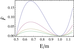
Note that such DF is negative for E<m/2𝐸𝑚2E<m/2, so, in principle, we would have to restrict its domain to values of energy larger than m/2𝑚2m/2. In the next section we show that a natural way to do this is by constraining the values of the free parameter ϕosubscriptitalic-ϕ𝑜\phi_{o}. In figure 2 we plot the behavior of the DF given by (32), once ϕosubscriptitalic-ϕ𝑜\phi_{o} has been chosen adequately.

Refer to caption
Figure 2: Dimensionless DF, F~=ξo1~𝐹superscriptsubscript𝜉𝑜1\tilde{F}=\xi_{o}^{-1}\mathcal{F}, for the general relativistic extension of Hernquist potential as a function of E/m𝐸𝑚E/m, for different values of L/m𝐿𝑚L/m: 0.2 (blue), 0.5 (violet), 1 (yellow), 1.5 (green).

Constraining the values for ϕosubscriptitalic-ϕ𝑜\phi_{o}

Self-gravitation equations (19)-(21) impose some restrictions to the stress-energy tensor (not necessarily equivalent to energy conditions), when one demands that 00\mathcal{F}\geq 0. They can be summarized as,

Tμνsubscript𝑇𝜇𝜈\displaystyle T_{\mu\nu} 0,absent0\displaystyle\geq 0, (34a)
T𝑇\displaystyle T 0,absent0\displaystyle\leq 0, (34b)

Indeed these restrictions are stronger than the weak, null, dominant and strong energy conditions. When they are applied to the stress-energy tensor given by (5)-(7), we find the following inequality

0f1/2,0𝑓12{}0\leq f\leq 1/2, (35)

which in terms of the radial coordinate r𝑟r is equivalent to state that

ra(ϕo1).𝑟𝑎subscriptitalic-ϕ𝑜1r\geq a\left(\phi_{o}-1\right).

This means that a real, positive DF, determining the stress-energy tensor could be well defined only for ra(ϕo1)𝑟𝑎subscriptitalic-ϕ𝑜1r\geq a\left(\phi_{o}-1\right). So, the maximum value of ϕosubscriptitalic-ϕ𝑜\phi_{o} that permits a DF well defined at the entire configuration space, r0𝑟0r\geq 0, is ϕo=1subscriptitalic-ϕ𝑜1\phi_{o}=1.

The bounding value for ϕosubscriptitalic-ϕ𝑜\phi_{o} can be diminished by taking into account that the DF of eq. (32) is negative for E<m/2𝐸𝑚2E<m/2 and remembering that the minimum value for a particle’s energy is Emin=mAsubscript𝐸min𝑚𝐴E_{\text{min}}=m\sqrt{A}. Therefore, situations where A<1/2𝐴12\sqrt{A}<1/2, which in this case equals to state that r<a(3ϕ0/21)𝑟𝑎3subscriptitalic-ϕ021r<a(3\phi_{0}/2-1), are not described for a positive DF given by (32). Such a DF only could describe situations where

ra(3ϕ021),𝑟𝑎3subscriptitalic-ϕ021r\geq a\left(\frac{3\phi_{0}}{2}-1\right),

which means that, ϕo=2/3subscriptitalic-ϕ𝑜23\phi_{o}=2/3 is now the maximum value for ϕosubscriptitalic-ϕ𝑜\phi_{o} such that \mathcal{F} is positive and well defined for r0𝑟0r\geq 0. By choosing this bound for ϕosubscriptitalic-ϕ𝑜\phi_{o} we guarantee that Em/2𝐸𝑚2E\geq m/2 for all situations. Thus, finally we can state that the set of values for the free parameter ϕosubscriptitalic-ϕ𝑜\phi_{o} are given by

  0ϕo2/3,  0subscriptitalic-ϕ𝑜23\boxed{\>\>0\leq\phi_{o}\leq 2/3\>\>}\>\>, (36)

in order to obtain a self-consistent relativistic Hernquist model, charaterized by a DF well defined at the entire configuration space.

V Distribution Functions for a general-relativistic version of the Hypervirial family

The formalism used in the preceding sections can also be applied in the case of the hypervirial family, to which Hernquist model belongs. In Newtonian gravity, the hipervirial potentials are given by

ϕn(r)=ϕno[1+(r/a)n]1n,subscriptitalic-ϕ𝑛𝑟subscriptitalic-ϕ𝑛𝑜superscriptdelimited-[]1superscript𝑟𝑎𝑛1𝑛\phi_{n}(r)=-\frac{\phi_{no}}{\left[1+\left(r/a\right)^{n}\right]^{\frac{1}{n}}}, (37)

where n𝑛n is a positive integer and ϕnosubscriptitalic-ϕ𝑛𝑜\phi_{no}, a𝑎a positive real constants. Each member is characterized by a DF proportional to E(3n+1)/2Ln2superscript𝐸3𝑛12superscript𝐿𝑛2E^{(3n+1)/2}L^{n-2}.

As in the case of Hernquist model (the particular case n=1𝑛1n=1 of (37)), a physically reasonable relativistic extension, introduced previously in Nguyen and Lingam (2013), is performed by defining f=ϕn/2𝑓subscriptitalic-ϕ𝑛2f=-\phi_{n}/2 in relation (2), leading to a stress-energy tensor of the form

Trrsuperscript𝑇𝑟𝑟\displaystyle T^{rr} =\displaystyle= 22n1f2n+2πanϕno2nGr2n(1f)(1+f)9=2r2nTθθsuperscript22𝑛1superscript𝑓2𝑛2𝜋superscript𝑎𝑛superscriptsubscriptitalic-ϕ𝑛𝑜2𝑛𝐺superscript𝑟2𝑛1𝑓superscript1𝑓92superscript𝑟2𝑛superscript𝑇𝜃𝜃\displaystyle\frac{2^{2n-1}f^{2n+2}}{\pi a^{n}{\phi_{no}}^{2n}Gr^{2-n}(1-f)(1+f)^{9}}=\frac{2r^{2}}{n}T^{\theta\theta} (38)
=\displaystyle= f(1f)(n+1)(1+f)6Ttt,𝑓1𝑓𝑛1superscript1𝑓6superscript𝑇𝑡𝑡\displaystyle\frac{f(1-f)}{(n+1)(1+f)^{6}}T^{tt},

and Tμν=0superscript𝑇𝜇𝜈0T^{\mu\nu}=0 for μν𝜇𝜈\mu\neq\nu. From (38) is easy to see that Pθ=(n/2)Prsubscript𝑃𝜃𝑛2subscript𝑃𝑟P_{\theta}=(n/2)P_{r}, which, by using Proposition 1, implies that the corresponding DF can be written as

=ξ(E)Ln2,n=1,2,formulae-sequence𝜉𝐸superscript𝐿𝑛2𝑛12\mathcal{F}=\xi(E)L^{n-2},\qquad n=1,2,...

By introducing the above expression into (19)-(21) we obtain

mAmξ(E)E2(E2Am2)n12dE=2A3/2(1A)2n+1,superscriptsubscript𝑚𝐴𝑚superscript𝜉𝐸superscript𝐸2superscriptsuperscript𝐸2𝐴superscript𝑚2𝑛12differential-d𝐸2superscript𝐴32superscript1𝐴2𝑛1\int\limits_{m\sqrt{A}}^{m}{\xi^{*}(E)E^{2}}\left(\frac{E^{2}}{A}-m^{2}\right)^{\frac{n-1}{2}}\mathrm{d}E=2A^{3/2}\left(1-\sqrt{A}\right)^{2n+1},
mAmξ(E)(E2Am2)n+12dE=(1A)2n+2,superscriptsubscript𝑚𝐴𝑚superscript𝜉𝐸superscriptsuperscript𝐸2𝐴superscript𝑚2𝑛12differential-d𝐸superscript1𝐴2𝑛2\int\limits_{m\sqrt{A}}^{m}\xi^{*}(E)\left(\frac{E^{2}}{A}-m^{2}\right)^{\frac{n+1}{2}}\mathrm{d}E=\left(1-\sqrt{A}\right)^{2n+2},

where

ξ(E)=ξ(E)(n+1)Γ(n+12)24π52anϕno2nGΓ(n2)m.𝜉𝐸superscript𝜉𝐸𝑛1Γ𝑛12superscript24superscript𝜋52superscript𝑎𝑛superscriptsubscriptitalic-ϕ𝑛𝑜2𝑛𝐺Γ𝑛2𝑚\xi(E)=\xi^{*}(E)\frac{\left(n+1\right)\Gamma\left(\frac{n+1}{2}\right)}{2^{4}\pi^{\frac{5}{2}}a^{n}{\phi_{no}}^{2n}G\Gamma\left(\frac{n}{2}\right)m}.

These two relations are essentially the same: the first one can be obtained by taking the derivative of the second one with respect to A𝐴\sqrt{A}. So, in this case, we can choose the second one relation (the simpler one) as the integral equation to be solved, in order to find an explicit expression for function ξ𝜉\xi. Here, for simplicity, we define A=x𝐴𝑥\sqrt{A}=x, which leads to

mxmξ(E)[(Em)2x2]n+12dE=(xm)n+1(1x)2n+2.superscriptsubscript𝑚𝑥𝑚superscript𝜉𝐸superscriptdelimited-[]superscript𝐸𝑚2superscript𝑥2𝑛12differential-d𝐸superscript𝑥𝑚𝑛1superscript1𝑥2𝑛2\int\limits_{mx}^{m}\xi^{*}(E)\left[{{\left(\frac{E}{m}\right)}^{2}}-{x}^{2}\right]^{\frac{n+1}{2}}\mathrm{d}E=\left(\frac{x}{m}\right)^{n+1}\left(1-x\right)^{2n+2}. (39)

In order to solve the above relation it is convenient to consider, separately, two cases: (i) n=1,3,5,𝑛135n=1,3,5,... and (ii) n=0,2,4,𝑛024n=0,2,4,.... Each of these options will lead to two kinds of distribution functions.

  1. (i)

    By choosing n=2p+1𝑛2𝑝1n=2p+1, for p=0,1,2,𝑝012p=0,1,2,\ldots, in eq. (39), we find that

    ξ2p+1(E)=k=14p+4a2p+1(Em)k1,subscript𝜉2𝑝1𝐸superscriptsubscript𝑘14𝑝4subscript𝑎2𝑝1superscript𝐸𝑚𝑘1\xi_{2p+1}(E)=\sum\limits_{k=1}^{4p+4}a_{2p+1}\left(\frac{E}{m}\right)^{k-1},

    where the a2p+1subscript𝑎2𝑝1a_{2p+1} are constants that will be specified later (see eq. (41)). Note that the DF corresponding to the relativistic extension of Hernquis model is obtained for p=0𝑝0p=0 (or n=1𝑛1n=1). The next case, p=1𝑝1p=1 (or n=3𝑛3n=3) is described by a function

    ξ3(E)(1Em)5[40(Em)231Em+5],proportional-tosubscript𝜉3𝐸superscript1𝐸𝑚5delimited-[]40superscript𝐸𝑚231𝐸𝑚5\xi_{3}(E)\propto\left(1-\frac{E}{m}\right)^{5}\left[40\left(\frac{E}{m}\right)^{2}-31\frac{E}{m}+5\right],

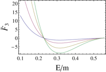
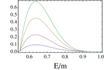
    which must be restricted to a domain given (approximately) by 0E/m0.22890𝐸𝑚0.22890\leq E/m\leq 0.2289 and 0.5461E/m10.5461𝐸𝑚10.5461\leq E/m\leq 1, in order to have a positive DF. For the other cases, p=2,3,..𝑝23p=2,3,.. the function ξ𝜉\xi also can be written in the form ξ2p+1(1ε)3p+2g(ε)proportional-tosubscript𝜉2𝑝1superscript1𝜀3𝑝2𝑔𝜀\xi_{2p+1}\propto(1-\varepsilon)^{3p+2}g(\varepsilon), where g𝑔g is a polynomial of degree p+1𝑝1p+1 in ε𝜀\varepsilon.

  2. (ii)

    The case in which n𝑛n is even, i.e. n=2p𝑛2𝑝n=2p for p=0,1,2,𝑝012p=0,1,2,\ldots in equation (39), demands a little more attention. By computing the derivative in x𝑥x of (39), p+1𝑝1p+1 times, we have

    mxmξ(E)dE(E/m)2x2(1xddx)p+1[x2p+1(1x)4p+2m2p+1(2p+1)!!].proportional-tosuperscriptsubscript𝑚𝑥𝑚𝜉𝐸d𝐸superscript𝐸𝑚2superscript𝑥2superscript1𝑥dd𝑥𝑝1delimited-[]superscript𝑥2𝑝1superscript1𝑥4𝑝2superscript𝑚2𝑝1double-factorial2𝑝1\int\limits_{mx}^{m}\frac{\xi(E)\mathrm{d}E}{\sqrt{\left(E/m\right)^{2}-x^{2}}}\propto\\ \left(-\frac{1}{x}\frac{\mathrm{d}}{\mathrm{d}x}\right)^{p+1}\left[\frac{x^{2p+1}\left(1-x\right)^{4p+2}}{m^{2p+1}(2p+1)!!}\right].

    Note that the right side has the form of an Abel integral, so the function ξ𝜉\xi can be determined explicitly by performing the Abel transformation. Thus, after some calculations we find

    ξ2p(E)=2Emk=04p+2b2pkEm1xk2x2(Em)2dx.subscript𝜉2𝑝𝐸2𝐸𝑚superscriptsubscript𝑘04𝑝2subscript𝑏2𝑝𝑘superscriptsubscript𝐸𝑚1superscript𝑥𝑘2superscript𝑥2superscript𝐸𝑚2differential-d𝑥{\xi_{2p}}(E)=\frac{2E}{m}\sum\limits_{k=0}^{4p+2}b_{2pk}\int\limits_{\frac{E}{m}}^{1}\frac{x^{k-2}}{\sqrt{x^{2}-\left(\frac{E}{m}\right)^{2}}}\mathrm{d}x.

    where b2pksubscript𝑏2𝑝𝑘b_{2pk} are constants given by relations (43). For example, the case p=1𝑝1p=1 (or n=2𝑛2n=2), for which the L𝐿L-dependence is dropped, lead us to the DF corresponding to the relativistic extension of the Plummer model:

    ξ2E11E2m2+84π1E2m2(1733E3m7+1274Em5)154π(21E5m9+140E3m7+40Em5)ln(mE1E2m2+mE)missing-subexpressionproportional-tosubscript𝜉2superscript𝐸11superscript𝐸2superscript𝑚284𝜋1superscript𝐸2superscript𝑚21733superscript𝐸3superscript𝑚71274𝐸superscript𝑚5missing-subexpressionmissing-subexpressionmissing-subexpression154𝜋21superscript𝐸5superscript𝑚9140superscript𝐸3superscript𝑚740𝐸superscript𝑚5𝑚𝐸1superscript𝐸2superscript𝑚2𝑚𝐸\begin{array}[]{cc}&\xi_{2}\propto E^{-1}\sqrt{1-\frac{E^{2}}{m^{2}}}+\frac{8}{4\pi}\sqrt{1-\frac{E^{2}}{m^{2}}}\left(\frac{1733E^{3}}{m^{7}}+\frac{1274E}{m^{5}}\right)\\ &\\ &-\frac{15}{4\pi}\left(\frac{21E^{5}}{m^{9}}+\frac{140E^{3}}{m^{7}}+\frac{40E}{m^{5}}\right)\ln\left(\frac{m}{E}\sqrt{1-\frac{E^{2}}{m^{2}}}+\frac{m}{E}\right)\end{array}

We can summarize our results through the following relations

n(odd)=ln2k=12n+2ankϵk1,n=1,3,5,formulae-sequencesuperscriptsubscript𝑛oddsuperscript𝑙𝑛2superscriptsubscript𝑘12𝑛2subscript𝑎𝑛𝑘superscriptitalic-ϵ𝑘1𝑛135\mathcal{F}_{n}^{(\text{odd})}=l^{n-2}\sum\limits_{k=1}^{2n+2}a_{nk}\epsilon^{k-1},\qquad n=1,3,5,... (40)

where

anksubscript𝑎𝑛𝑘\displaystyle a_{nk} =\displaystyle= (2n+2k)(1)k+n12(k+n+1)!!k24π3anϕno2nGm5Γ(n2)k!!(n+1)!!binomial2𝑛2𝑘superscript1𝑘𝑛12double-factorial𝑘𝑛1𝑘superscript24superscript𝜋3superscript𝑎𝑛superscriptsubscriptitalic-ϕ𝑛𝑜2𝑛𝐺superscript𝑚5Γ𝑛2double-factorial𝑘double-factorial𝑛1\displaystyle\binom{2n+2}{k}\frac{(-1)^{k+\frac{n-1}{2}}(k+n+1)!!k}{2^{4}\pi^{3}a^{n}{\phi_{no}}^{2n}Gm^{5}\Gamma\left(\frac{n}{2}\right)k!!(n+1)!!} (41)
×\displaystyle\times (n+1)πΓ(n+12),n=1,3,5,..,formulae-sequence𝑛1𝜋Γ𝑛12𝑛135\displaystyle(n+1)\sqrt{\pi}\Gamma\left(\frac{n+1}{2}\right),\>\>n=1,3,5,..,

for DFs with odd index, and

n(even)=ln2ϵk=02n+2bnkϵ1xk2dxx2ϵ2,n=0,2,4,,formulae-sequencesuperscriptsubscript𝑛evensuperscript𝑙𝑛2italic-ϵsuperscriptsubscript𝑘02𝑛2subscript𝑏𝑛𝑘superscriptsubscriptitalic-ϵ1superscript𝑥𝑘2d𝑥superscript𝑥2superscriptitalic-ϵ2𝑛024\mathcal{F}_{n}^{(\text{even})}=l^{n-2}\epsilon\sum\limits_{k=0}^{2n+2}b_{nk}\int\limits_{\epsilon}^{1}\frac{x^{k-2}\mathrm{d}x}{\sqrt{x^{2}-\epsilon^{2}}},\qquad n=0,2,4,..., (42)

where

bn0=(1)1n2(n+1)Γ(n+12)23π3anϕno2nGm5πΓ(n2),bn1=0,formulae-sequencesubscript𝑏𝑛0superscript11𝑛2𝑛1Γ𝑛12superscript23superscript𝜋3superscript𝑎𝑛superscriptsubscriptitalic-ϕ𝑛𝑜2𝑛𝐺superscript𝑚5𝜋Γ𝑛2subscript𝑏𝑛10b_{n0}=\frac{(-1)^{1-\frac{n}{2}}(n+1)\Gamma\left(\frac{n+1}{2}\right)}{2^{3}\pi^{3}a^{n}{\phi_{no}}^{2n}Gm^{5}\sqrt{\pi}\Gamma\left(\frac{n}{2}\right)},\qquad b_{n1}=0,
bnksubscript𝑏𝑛𝑘\displaystyle b_{nk} =\displaystyle= (2n+2k)(k+n+1)!!(1)kn2(k1)23π3anϕno2nGm5(k1)!!(n+1)!!binomial2𝑛2𝑘double-factorial𝑘𝑛1superscript1𝑘𝑛2𝑘1superscript23superscript𝜋3superscript𝑎𝑛superscriptsubscriptitalic-ϕ𝑛𝑜2𝑛𝐺superscript𝑚5double-factorial𝑘1double-factorial𝑛1\displaystyle\binom{2n+2}{k}\frac{{(k+n+1)!!}(-1)^{k-\frac{n}{2}}(k-1)}{2^{3}\pi^{3}a^{n}{\phi_{no}}^{2n}Gm^{5}(k-1)!!(n+1)!!} (43)
×\displaystyle\times (n+1)Γ(n+12)πΓ(n2),k2,n=0,2,4,formulae-sequence𝑛1Γ𝑛12𝜋Γ𝑛2𝑘2𝑛024\displaystyle\frac{(n+1)\Gamma\left(\frac{n+1}{2}\right)}{\sqrt{\pi}\Gamma\left(\frac{n}{2}\right)},\>\>\;k\geq 2,\>\>n=0,2,4,...
Refer to caption
Refer to caption
Refer to caption
Figure 3: Dimensionless DF corresponding to the hypervirial model n=3𝑛3n=3, for different values of L/m𝐿𝑚L/m: 0.2 (blue), 0.5 (violet), 1 (yellow), 1.5 (green). This DF is positive for 0E/m0.22890𝐸𝑚0.22890\leq E/m\leq 0.2289 (left) and for 0.5461E/m10.5461𝐸𝑚10.5461\leq E/m\leq 1 (central panel). Note that probability density reaches higher values in the first range. For E/m>1𝐸𝑚1E/m>1, this DF has negative values (right panel).
Refer to caption
Refer to caption
Refer to caption
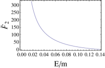
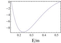
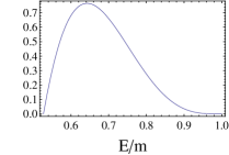
Figure 4: Dimensionless DF corresponding to the hypervirial model n=2𝑛2n=2, which is a relativistic extension of Plummer model. The DF is positive for 0E/m0.13880𝐸𝑚0.13880\leq E/m\leq 0.1388 (left panel) and 0.5270E/m<10.5270𝐸𝑚10.5270\leq E/m<1 (right panel) and is negative for 0.1388<E/m<0.52700.1388𝐸𝑚0.52700.1388<E/m<0.5270 (central panel).
Refer to caption
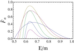
Figure 5: Dimensionless DF, F~n=25m5π3Gϕno2nannsubscript~𝐹𝑛superscript25superscript𝑚5superscript𝜋3𝐺subscriptsuperscriptitalic-ϕ2𝑛𝑛𝑜superscript𝑎𝑛subscript𝑛\tilde{F}_{n}=2^{5}m^{5}\pi^{3}G{\phi}^{2n}_{no}a^{n}\mathcal{F}_{n}, for the general relativistic extension of the Hypervirial family as a function of E/m𝐸𝑚E/m with L/m=2𝐿𝑚2L/m=2, for different values of n𝑛n: n=1 (red), n=2 (Blue), n=3(Green), n=5 (Orange), n=7 (Purple), n=9 (Brown).
Table 1: Upper bound value of ϕnosubscriptitalic-ϕ𝑛𝑜\phi_{no} for different n𝑛n.
    n ϕnosubscriptitalic-ϕ𝑛𝑜\phi_{no}
   1 2/3
   2 0.619472
   3 0.587143
   5 0.544734
   7 0.517533
   9 0.498276

As done in Sec. IV, we can choose the values of ϕnosubscriptitalic-ϕ𝑛𝑜\phi_{no} so that nsubscript𝑛\mathcal{F}_{n} be positive everywhere in configuration space, r>0𝑟0r>0. Figure 5 suggests that the upper bound for ϕnosubscriptitalic-ϕ𝑛𝑜\phi_{no} decreases with n𝑛n, as confirmed by the values of Table 1.

VI Conclusion

We derived an analytic expression for the DF corresponding to the general relativistic extension of the Hernquist model presented in Nguyen and Lingam (2013). In the derivation we considered the self-gravitating equations for asymptotically flat static isotropic space-times, from which we established that anisotropic models so that Pθ=kPrsubscript𝑃𝜃𝑘subscript𝑃𝑟P_{\theta}=kP_{r}, with k𝑘k constant, are characterized by a DF of the form =ξ(E)L2(k1)𝜉𝐸superscript𝐿2𝑘1\mathcal{F}=\xi(E)L^{2\left(k-1\right)} (proposition 1). For the Hernquist case, corresponding to k=1/2𝑘12k=1/2, we find (E,L)L1(2E/m1)(1E/m)2proportional-to𝐸𝐿superscript𝐿12𝐸𝑚1superscript1𝐸𝑚2\mathcal{F}(E,L)\propto L^{-1}\left(2{E}/{m}-1\right)\left(1-{E}/{m}\right)^{2}, from which we established that the upper bound of free parameter ϕosubscriptitalic-ϕ𝑜\phi_{o} is 2/3232/3 (lesser than the one obtained in Nguyen and Lingam (2013)), in order to have a DF defined at the entire configuration space, r>0𝑟0r>0.

Exploiting our experience with the Hernquist potential we also derived analytic expressions for the DF of the Hypervirial family, which satisfies Pθ=(n/2)Prsubscript𝑃𝜃𝑛2subscript𝑃𝑟P_{\theta}=(n/2)P_{r} for the n𝑛nth member (Hernquist model is the first member, n=1𝑛1n=1). Proposition 1 implies that the DF corresponding to the n𝑛nth member is of the form n=ξn(E)L2nsubscript𝑛subscript𝜉𝑛𝐸superscript𝐿2𝑛\mathcal{F}_{n}=\xi_{n}(E)L^{2-n}, where we have to distinguish between odd and even values of n𝑛n, in order to encompass in a simple fashion all cases (eqs. (40) and (42)). Thus we find two subfamilies in the set of hypervirial models, which now can be regarded as a self-consistent family of models in the context of general relativity.

We note that the free parameter ϕnosubscriptitalic-ϕ𝑛𝑜\phi_{no}, corresponding to the n𝑛nth member of the hypervirial family, has an upper bound which diminishes by increasing n𝑛n. Such upper bound, as in the case of Hernquist model, was chosen in such a way that the DF was positive for r>0𝑟0r>0. However, one could choose different upper bounds for these parameters when taking into account a reduced configuration space, for example given by rr𝑟subscript𝑟r\geq r_{*}, where rsubscript𝑟r_{*} is a positive constant. This can be used to model situations composed by two solutions of Einstein equations, one of them defined in 0<r<r0𝑟subscript𝑟0<r<r_{*} (the solution inside the region bounded by the shell r=r𝑟subscript𝑟r=r_{*}) and the other one, an Hypervirial solution, defined in rr𝑟subscript𝑟r\geq r_{*}. In such a case, the DF has to be defined by parts and junction conditions has to be satisfied in the shell r=r𝑟subscript𝑟r=r_{*} (see for example Das et al. (2003)).

Appendix A Hernquist potential in Newtonian Gravity

The distribution function (DF) for the Hernquist potential is given by Nguyen and Lingam (2013)

(ε,L)=AεβL2α𝜀𝐿𝐴superscript𝜀𝛽superscript𝐿2𝛼\mathcal{F}(\varepsilon,L)=A{\varepsilon}^{\beta}L^{2\alpha} (44)

where L𝐿L is the norm of the specific angular momentum and ε=ϕE𝜀subscriptitalic-ϕ𝐸\varepsilon=\phi_{*}-E is the relative energy (in this case we have to set ϕ=0subscriptitalic-ϕ0\phi_{*}=0). This is the same distribution function used by Nguyen et al. in order to develop a family of potential-density pairs, including the Hernquist model as a particular case. The mass density can be found by integrating the distribution function over the velocity space,

ρ=(ε,L)d3ν,𝜌𝜀𝐿superscriptd3𝜈\rho=\int\mathcal{F}(\varepsilon,L){\mathrm{d}}^{3}\nu,

which, by introducing (44) and using spherical coordinates, leads to

ρ=02π0π0νeAεβL2αν2sinηdνdηdκ𝜌superscriptsubscript02𝜋superscriptsubscript0𝜋superscriptsubscript0subscript𝜈𝑒𝐴superscript𝜀𝛽superscript𝐿2𝛼superscript𝜈2𝜂d𝜈d𝜂d𝜅\rho=\int_{0}^{2\pi}\int_{0}^{\pi}\int_{0}^{\nu_{e}}A{\varepsilon}^{\beta}L^{2\alpha}\nu^{2}\sin\eta{\mathrm{d}}\nu{\mathrm{d}}\eta{\mathrm{d}}\kappa (45)

where νe=2ϕsubscript𝜈𝑒2italic-ϕ\nu_{e}=\sqrt{-2\phi} is the escape velocity and ϕitalic-ϕ\phi is the gravitational potential. Since in spherical coordinates we can write L2=r2ν2sin2ηsuperscript𝐿2superscript𝑟2superscript𝜈2superscript2𝜂L^{2}=r^{2}{\nu}^{2}\sin^{2}\eta and ε=E=ϕν2/2𝜀𝐸italic-ϕsuperscript𝜈22\varepsilon=-E=-\phi-\nu^{2}/2, we have

ρ=2πA0πsin2α+1ηdη0νe(ν22ϕ)βr2αν2α+2dν𝜌2𝜋𝐴superscriptsubscript0𝜋superscript2𝛼1𝜂d𝜂superscriptsubscript0subscript𝜈𝑒superscriptsuperscript𝜈22italic-ϕ𝛽superscript𝑟2𝛼superscript𝜈2𝛼2differential-d𝜈\rho=2\pi A\int_{0}^{\pi}\sin^{2\alpha+1}\eta{\mathrm{d}}\eta\int_{0}^{\nu_{e}}\left(-\dfrac{\nu^{2}}{2}-\phi\right)^{\beta}r^{2\alpha}\nu^{2\alpha+2}{\mathrm{d}}\nu

The first integral above is basically a constant, so by taking 2πA0πsin2α+1ηdη=B2𝜋𝐴superscriptsubscript0𝜋superscript2𝛼1𝜂d𝜂𝐵2\pi A\int_{0}^{\pi}\sin^{2\alpha+1}\eta{\mathrm{d}}\eta=B, we have

ρ=Br2α0νe(ν22ϕ)βν2α+2dν𝜌𝐵superscript𝑟2𝛼superscriptsubscript0subscript𝜈𝑒superscriptsuperscript𝜈22italic-ϕ𝛽superscript𝜈2𝛼2differential-d𝜈\rho=Br^{2\alpha}\int_{0}^{\nu_{e}}\left(-\dfrac{\nu^{2}}{2}-\phi\right)^{\beta}\nu^{2\alpha+2}{\mathrm{d}}\nu (46)

Now, in order to compute the second integral, it can be cast as

ρ=Br2α02ϕϕβ(ν22ϕ1)βν2α+2dν,𝜌𝐵superscript𝑟2𝛼superscriptsubscript02italic-ϕsuperscriptitalic-ϕ𝛽superscriptsuperscript𝜈22italic-ϕ1𝛽superscript𝜈2𝛼2differential-d𝜈\rho=Br^{2\alpha}\int_{0}^{\sqrt{-2\phi}}\phi^{\beta}\left(-\dfrac{\nu^{2}}{2\phi}-1\right)^{\beta}\nu^{2\alpha+2}{\mathrm{d}}\nu,

where, by making the substitution x=ν2/ϕ𝑥superscript𝜈2italic-ϕx={\nu^{2}}/{\phi}, the integral becomes

ρ=Br2αϕβ+α+12α+1ϕ201(x1)βxα+1/2dx,𝜌𝐵superscript𝑟2𝛼superscriptitalic-ϕ𝛽𝛼1superscript2𝛼1italic-ϕ2superscriptsubscript01superscript𝑥1𝛽superscript𝑥𝛼12differential-d𝑥\rho=Br^{2\alpha}\phi^{\beta+\alpha+1}2^{\alpha+1}\sqrt{\dfrac{\phi}{2}}\int_{0}^{-1}{(-x-1)}^{\beta}x^{\alpha+1/2}{\mathrm{d}}x,

Again, the last integral is a constant. With this in mind and organizing the terms, we have

ρ=Cr2αϕβ+α+3/2𝜌𝐶superscript𝑟2𝛼superscriptitalic-ϕ𝛽𝛼32\rho=Cr^{2\alpha}\phi^{\beta+\alpha+3/2} (47)

Now it is possible to calculate the potential through the Poisson equation,

2ϕ=4πGρ=4πCGr2αϕβ+α+3/2superscript2italic-ϕ4𝜋𝐺𝜌4𝜋𝐶𝐺superscript𝑟2𝛼superscriptitalic-ϕ𝛽𝛼32{\nabla}^{2}\phi=4\pi G\rho=4\pi CGr^{2\alpha}\phi^{\beta+\alpha+3/2}

Since α𝛼\alpha and β𝛽\beta are parameters, it is straightforward to prove that

ϕ=ϕo1+r/a,italic-ϕsubscriptitalic-ϕ𝑜1𝑟𝑎\phi=-\dfrac{\phi_{o}}{1+r/a},

is a solution of the equation for α=1/2𝛼12\alpha=-1/2, β=2𝛽2\beta=2 and 4πCG=2/ϕo2a4𝜋𝐶𝐺2superscriptsubscriptitalic-ϕ𝑜2𝑎4\pi CG=-{2}/{{\phi_{o}}^{2}a}, where a𝑎a is the characteristic radius of the system.

Now returning to the expression (47) of the density and thus using the values α=1/2𝛼12\alpha=-1/2 and β=2𝛽2\beta=2, we can compute the constant A𝐴A:

C=2πA0πdη01(x1)2dx=2π2A3,𝐶2𝜋𝐴superscriptsubscript0𝜋differential-d𝜂superscriptsubscript01superscript𝑥12differential-d𝑥2superscript𝜋2𝐴3C=2\pi A\int_{0}^{\pi}{\mathrm{d}}\eta\int_{0}^{-1}{(-x-1)}^{2}{\mathrm{d}}x=-\dfrac{2\pi^{2}A}{3},

then

C=2π2A3=12πGϕo2a,𝐶2superscript𝜋2𝐴312𝜋𝐺superscriptsubscriptitalic-ϕ𝑜2𝑎C=-\dfrac{2\pi^{2}A}{3}=-\dfrac{1}{2\pi G{\phi_{o}}^{2}a},

which lead us to

A=34π3ϕo2aG𝐴34superscript𝜋3superscriptsubscriptitalic-ϕ𝑜2𝑎𝐺A=\dfrac{3}{4\pi^{3}{\phi_{o}}^{2}aG} (48)

In summary, we can establish that the distribution function, the gravitational potential and the mass density for the Hernquist model are given by

(ε,L)=34π3ϕo2aGε2L1𝜀𝐿34superscript𝜋3superscriptsubscriptitalic-ϕ𝑜2𝑎𝐺superscript𝜀2superscript𝐿1{}\mathcal{F}(\varepsilon,L)=\dfrac{3}{4\pi^{3}{\phi_{o}}^{2}aG}{\varepsilon}^{2}L^{-1} (49)
ϕ=ϕo1+r/aitalic-ϕsubscriptitalic-ϕ𝑜1𝑟𝑎\phi=-\dfrac{\phi_{o}}{1+r/a} (50)
ρ=12πGϕo2ar1ϕ3=ϕo2πGar(11+r/a)3𝜌12𝜋𝐺superscriptsubscriptitalic-ϕ𝑜2𝑎superscript𝑟1superscriptitalic-ϕ3subscriptitalic-ϕ𝑜2𝜋𝐺𝑎𝑟superscript11𝑟𝑎3\rho=-\dfrac{1}{2\pi G{\phi_{o}}^{2}a}r^{-1}{\phi}^{3}=\dfrac{\phi_{o}}{2\pi Gar}\left(\dfrac{1}{1+r/a}\right)^{3} (51)

Appendix B Demonstration of Lemma 1

In this appendix we provide a proof by reductio ad absurdum of lemma 1, used to obtain theorem 1:

Lemma 1

If \mathcal{F} is a DF satisfying the self-gravitation equations (19), (20) and (21), then limL0(L2)=0subscript𝐿0superscript𝐿20\lim\limits_{L\rightarrow 0}\left(L^{2}\mathcal{F}\right)=0.

Proof. If one supposes that

limL0(L2)0,subscript𝐿0superscript𝐿20\lim\limits_{L\rightarrow 0}\left(L^{2}\mathcal{F}\right)\neq 0,

then, from the definition of limit, for every δ>0𝛿0\delta>0 there exists ϵ>0italic-ϵ0\epsilon>0 and L0subscript𝐿0L_{0} such that 0<L0<δ0subscript𝐿0𝛿0<L_{0}<\delta and (E,L0)>ϵL02𝐸subscript𝐿0italic-ϵsuperscriptsubscript𝐿02\mathcal{F}(E,L_{0})>\epsilon{L_{0}}^{-2}.

On the other hand, since \mathcal{F} must be a continuous function, then L2superscript𝐿2L^{2}\mathcal{F} is a continuous function too, so there exists a region centered in L0subscript𝐿0L_{0} such that >ϵL2italic-ϵsuperscript𝐿2\mathcal{F}>\epsilon{L}^{-2}, i.e. >ϵL2italic-ϵsuperscript𝐿2\mathcal{F}>\epsilon{L}^{-2} for every L𝐿L belonging to L0δL<L<L0+δLsubscript𝐿0𝛿𝐿𝐿subscript𝐿0𝛿𝐿L_{0}-\delta L<L<L_{0}+\delta L.

All of the above holds for every choice of 0<δ<δL0𝛿𝛿𝐿0<\delta<\delta L. Then, if we choose δ𝛿\delta in such a way that 0<L<δ0𝐿𝛿0<L<\delta and, therefore, L𝐿L falls inside the interval (L0δL,L0+δL)subscript𝐿0𝛿𝐿subscript𝐿0𝛿𝐿(L_{0}-\delta L,L_{0}+\delta L), then for such δ𝛿\delta there exists an ϵ>0italic-ϵ0\epsilon>0 such that whenever 0<L<δ0𝐿𝛿0<L<\delta we have >ϵL2italic-ϵsuperscript𝐿2\mathcal{F}>\epsilon L^{-2}.

Now, by choosing Lmsubscript𝐿𝑚L_{m} to be smaller than δ𝛿\delta, we can write

0Lm(E,L)LdLLm2L2ϵ0LmdLLLm2L2.subscriptsuperscriptsubscript𝐿𝑚0𝐸𝐿𝐿d𝐿superscriptsubscript𝐿𝑚2superscript𝐿2italic-ϵsubscriptsuperscriptsubscript𝐿𝑚0d𝐿𝐿superscriptsubscript𝐿𝑚2superscript𝐿2\int^{L_{m}}_{0}\frac{\mathcal{F}(E,L)L\mathrm{d}L}{\sqrt{{L_{m}}^{2}-L^{2}}}\geq\epsilon\int^{L_{m}}_{0}\frac{\mathrm{d}L}{L\sqrt{{L_{m}}^{2}-L^{2}}}.

Note that the right hand side integral does not converge and the left hand side integral must converge since ρ𝜌\rho, given by (23), is finite. This means that the relation above is an absurd, which leads us to state that

limL0(L2)=0.formulae-sequencesubscript𝐿0superscript𝐿20\hfill\lim\limits_{L\rightarrow 0}\left(L^{2}\mathcal{F}\right)=0.\hfill\blacksquare

References

  • Lemos and Letelier (1993) J. P. S. Lemos and P. S. Letelier, Phys. Rev. D 10, L75 (1993).
  • Lemos and Letelier (1994) J. P. S. Lemos and P. S. Letelier, Phys. Rev. D 49, 5135 (1994).
  • González and Letelier (2000) G. A. González and P. S. Letelier, Phys. Rev. D 62, 064025 (2000).
  • Semerák and Zácek (2000) O. Semerák and M. Zácek, Phys. Rev. D 17, 1613 (2000).
  • Semerák (2002) O. Semerák, Classical and Quantum Gravity 19, 3829 (2002).
  • Zácek and Semerák (2002) M. Zácek and O. Semerák, Czechoslovak Journal of Physics 52, 19 (2002).
  • Vogt and Letelier (2005) D. Vogt and P. S. Letelier, Mon. Not. R. Astron. Soc. 363, 268 (2005), eprint astro-ph/0507406.
  • Cooperstock and Tieu (2007) F. I. Cooperstock and S. Tieu, International Journal of Modern Physics A 22, 2293 (2007).
  • Ramos-Caro and González (2008) J. Ramos-Caro and G. A. González, Classical and Quantum Gravity 25, 045011 (2008).
  • Lora-Clavijo et al. (2010) F. D. Lora-Clavijo, P. A. Ospina-Henao, and J. F. Pedraza, Phys. Rev. D 82, 084005 (2010).
  • Ramos-Caro et al. (2012) J. Ramos-Caro, C. A. Agón, and J. F. Pedraza, Phys. Rev. D 86, 043008 (2012).
  • Carrick and Cooperstock (2012) J. D. Carrick and F. I. Cooperstock, Astrophysics and Space Science 337, 321 (2012).
  • Rodrigues (2012) D. C. Rodrigues, Journal of Cosmology and Astroparticle Physics 09, 031 (2012).
  • Herrera-Aguilar and Nucamendi (2014) A. Herrera-Aguilar and U. Nucamendi, Journal of Physics: Conference Series 545, 012006 (2014).
  • Binney and McMillan (2011) J. Binney and P. McMillan, Mon. Not. R. Astron. Soc. 413, 1889 (2011).
  • Binney (2010) J. Binney, Mon. Not. R. Astron. Soc. 401, 2318 (2010).
  • Plummer (1911) H. C. Plummer, Mon. Not. R. Astron. Soc. 71, 460 (1911).
  • Eddington (1916) A. S. Eddington, Mon. Not. R. Astron. Soc. 76, 572 (1916).
  • Lynden-Bell (1962) D. Lynden-Bell, Mon. Not. R. Astron. Soc. 123, 447 (1962).
  • Jaffe (1983) W. Jaffe, Mon. Not. R. Astron. Soc. 202, 995 (1983).
  • Binney and Tremaine (2008) J. Binney and S. Tremaine, Galactic Dynamics (Princeton Univ. Press, Princeton, NJ, 2008), 2nd ed.
  • Hernquist (1990) L. Hernquist, Astrophys. J. 356, 359 (1990).
  • Pedraza et al. (2012) J. F. Pedraza, J. Ramos-Caro, and G.A. González, Mon. Not. R. Astron. Soc. 390, 1587 (2008).
  • Bowers and Liang (1974) R. L. Bowers and E. P. T. Liang, Astrophys. J. 188, 657 (1974).
  • Bayin (1982) S.S. Bayin, Phys. Rev. D 26, 1262 (1982).
  • Singh et al. (2012) T. Singh, G. P. Singh, and R. S. Srivastava, International Journal of Theoretical Physics 31, 545 (1992).
  • Coley and Tupper (1994) A. A. Coley and B. O. J. Tupper, Classical and Quantum Gravity 11, 2553 (1994).
  • Das et al. (2012) A. Das, N. Tariq, D. Aruliah and T. Biech, Journal of Mathematical Physics 38, 4202 (1997).
  • Herrera and Santos (1997) L. Herrera and N. O. Santos, Phys. Rep. 286, 53 (1997).
  • Herrera et al. (2012) L. Herrera, A. Di Prisco, J.L. Hernández-Pastora and N.O. Santos, Physics Letters A 237, 113 (1998).
  • Corchero (1998) E.S. Corchero, Classical and Quantum Gravity 15, 3645 (1998).
  • Das and Kloster (2000) A. Das and S. Kloster, Phys. Rev. D 62, 104002 (2000).
  • Dev and Gleiser (2002) K. Dev and M. Gleiser, General Relativity and Gravitation 34, 1793 (2002).
  • Hernández and Nuñez (2004) H. Hernández and L. A. Nuñez, Canadian Journal of Physics 82, 29 (2004).
  • Mak and Harko (2003) M.K. Mak and T. Harko, Proceedings of the Royal Society of London A: Mathematical, Physical and Engineering Sciences 459, 393 (2003).
  • Herrera et al. (2004) L. Herrera, A. Di Prisco, J. Martin J. Ospino N.O. Santos and O. Troconis, Phys. Rev. D 69, 084026 (2004).
  • Maharaj and Chaisi (2006) S. D. Maharaj and M. Chaisi, General Relativity and Gravitation 38, 1723 (2006).
  • Maharaj and Chaisi (2006) S. D. Maharaj and M. Chaisi, Mathematical Methods in the Applied Sciences 29, 67 (2006).
  • Herrera et al. (2008) L. Herrera, J. Ospino and A. Di Prisco, Phys. Rev. D 77, 027502 (2008).
  • Sharma and Tikekar (2012) R. Sharma and R. Tikekar, General Relativity and Gravitation 44, 2503 (2012).
  • Le Delliou et al. (2013) M. Le Delliou, J. P. Mimoso, F. C. Mena M. Fontanini D. C. Guariento and E. Abdalla, Phys. Rev. D 88, 027301 (2013).
  • Herrera and Barreto (2013) L. Herrera and W. Barreto, Phys. Rev. D 87, 087303 (2013).
  • Sgró et al. (2013) M. A. Sgró, D. J. Paz and M. Merchán, Mon. Not. R. Astron. Soc. 433, 787 (2013).
  • Nguyen and Pedraza (2013) P. H. Nguyen and J. F. Pedraza, Phys. Rev. D 88, 064020 (2013).
  • Nguyen and Lingam (2013) P. H. Nguyen and M. Lingam, Mon. Not. R. Astron. Soc. 436, 2014 (2013).
  • Evans and An (2005) N. W. Evans and J. An, Mon. Not. R. Astron. Soc. 360, 492 (2005).
  • Andréasson (2011) H. Andréasson, Living Reviews in Relativity 14, 4 (2011).
  • Weinberg (1972) S. Weinberg, Gravitation and Cosmology (John Wiley and Sons Ltd, New York, 1972).
  • Buchdahl (1964) H. A. Buchdahl, Astrophys. J. 140, 1512 (1964).
  • Vogt and Letelier (2010) D. Vogt and P. S. Letelier, Mon. Not. R. Astron. Soc. 402, 1313 (2010).
  • Vogt and Letelier (2010) D. Vogt and P. S. Letelier, Mon. Not. R. Astron. Soc. 406, 2689 (2010).
  • Cercignani and Kremer (2002) C. Cercignani and G. M. Kremer, The Relativistic Boltzmann Equation: Theory and Applications (Birkhäuser, Basel, 2002).
  • Straumann (2013) N. Straumann, General Relativity (Springer, Netherlands, 2013), 2nd ed.
  • Fackerell (1968) E. D. Fackerell, Astrophys. J. 153, 643 (1968).
  • Das et al. (2003) A. Das, A. De Benedictis and N. Tariq, Journal of Mathematical Physics 44, 5637 (2003).